Article

Comparison of Airborne LiDAR and Satellite Hyperspectral Remote Sensing to Estimate Vascular Plant Richness in Deciduous Mediterranean Forests of Central Chile

by
Andrés Ceballos
1,
Jaime Hernández
1,
Patricio Corvalán
1 and
Mauricio Galleguillos
1,2,*
1
Laboratory of Geomatics and Landscape Ecology, Forestry and Nature Conservation Faculty, University of Chile, Av. Santa Rosa 11315, La Pintana, Santiago, Chile
2
Department of Environmental Sciences, Faculty of Agronomic Sciences, University of Chile, Av. Santa Rosa 11315, La Pintana, Santiago, Chile
*
Author to whom correspondence should be addressed.
Remote Sens. 2015, 7(3), 2692-2714; https://doi.org/10.3390/rs70302692
Submission received: 1 September 2014 / Revised: 18 February 2015 / Accepted: 27 February 2015 / Published: 9 March 2015
(This article belongs to the Special Issue Earth Observation for Ecosystems Monitoring in Space and Time)

Abstract

:
The Andes foothills of central Chile are characterized by high levels of floristic diversity in a scenario, which offers little protection by public protected areas. Knowledge of the spatial distribution of this diversity must be gained in order to aid in conservation management. Heterogeneous environmental conditions involve an important number of niches closely related to species richness. Remote sensing information derived from satellite hyperspectral and airborne Light Detection and Ranging (LiDAR) data can be used as proxies to generate a spatial prediction of vascular plant richness. This study aimed to estimate the spatial distribution of plant species richness using remote sensing in the Andes foothills of the Maule Region, Chile. This region has a secondary deciduous forest dominated by Nothofagus obliqua mixed with sclerophyll species. Floristic measurements were performed using a nested plot design with 60 plots of 225 m2 each. Multiple predictors were evaluated: 30 topographical and vegetation structure indexes from LiDAR data, and 32 spectral indexes and band transformations from the EO1-Hyperion sensor. A random forest algorithm was used to identify relevant variables in richness prediction, and these variables were used in turn to obtain a final multiple linear regression predictive model (Adjusted R2 = 0.651; RSE = 3.69). An independent validation survey was performed with significant results (Adjusted R2 = 0.571, RMSE = 5.05). Selected variables were statistically significant: catchment slope, altitude, standard deviation of slope, average slope, Multiresolution Ridge Top Flatness index (MrRTF) and Digital Crown Height Model (DCM). The information provided by LiDAR delivered the best predictors, whereas hyperspectral data were discarded due to their low predictive power.

Graphical Abstract

1. Introduction

Biodiversity is an essential element from which all human populations benefit directly or indirectly [1]. The current and future state of biodiversity has acquired greater scientific and political relevance due to increasing knowledge of the adverse effects that its decrease may have on the ecosystem and the advantages this holds for the wellbeing of humankind [2,3,4].
The Andes foothills in central Chile are in one of the world’s biodiversity hotspots [5]. They have a high rate of floristic diversity and endemism [6], particularly in the transition zone between the Valdivian temperate rain forest and the sclerophyll forest in the Maule region [7,8], yet the region currently has very little area protected in the Chilean National System of Protected Wild Areas (SNASPE) or in other public protected areas such as nature sanctuaries, forest reserves or national parks, which currently comprise only 2% of the region’s total surface area [6]. Nevertheless, these ecosystems are extremely vulnerable, since they are subject to a sustained increase in anthropogenic pressure mainly related to the change in land use for agriculture and livestock and the illegal extraction of wood products from native forests [9,10,11]. Additionally, this area is prone to the effects being produced by climate change, with a significant decrease in rainfall and increase in air temperature [11,12,13]. The conservation of biodiversity must be a priority [9,14,15]. Therefore, rapid and objective methods must be developed to assess and predict biodiversity spatially [16]; observation by remote sensing plays a fundamental role here in light of its capacity to extrapolate point information about biodiversity collected in situ to different spatial and temporal scales [17].
Theoretical and empirical studies suggest that the biodiversity of a particular site is strongly influenced by and positively correlated with its environmental heterogeneity [18,19]. More complex environments can host a greater number of ecological niches, which, in turn, can be colonized and inhabited by a greater number of species [20,21,22]. Different remote sensors make it possible to capture spatial heterogeneity mainly from two perspectives: spatial heterogeneity (horizontal variability) and topographical-structural heterogeneity (vertical variability) [20].
On the one hand, a number of studies have associated the biodiversity of different sites with the information obtained by passive remote sensors [23,24,25,26,27], correlating biological diversity directly with spectral reflectance values [28], with different spectral vegetation indexes [19,25,29,30,31], and different types of feature extraction like principal components analysis (PCA) [32] or minimum noise fraction (MNF) [26]. Taking this into account, it is expected that hyperspectral sensors, which have great ability to detect characteristics associated with the biochemical, physiological, and structural spectral variability of the vegetation in the electromagnetic spectrum, will provide valuable information for the evaluation of biodiversity [33,34].
On the other hand, some studies have used topographical information, microreliefs and their spatial variability [35,36], along with the vertical structure of natural sites (understood as the configuration and variability of all the aboveground vegetation [20]) to estimate environmental heterogeneity, which is related to biodiversity. Topographical and structural information that an active LiDAR (Light Detection and Ranging) sensor is capable of capturing can be used to provide efficacious variables in studies on different ecosystems [37], especially forests with high vertical complexity [20]. It shows great potential for biodiversity characterization [26]. Within this context, combining LiDAR and hyperspectral data can be useful as they are related to different non-correlated proxies of plant biodiversity [38].
The concept of biodiversity involves many components (i.e., richness, relative abundance, composition, spatial distribution, functional ranges, different types like alpha, beta, and gamma diversity, etc.) associated with different taxonomic groups (plants, fungi, mammals, birds, reptiles, etc.), thereby rendering these systems complex and expensive to evaluate [4]. Maps of alpha diversity (i.e., species richness: the number of species associated with a known area) [39] generated using predictive models have proven to be a relevant tool for determining the biodiversity of a given area, for assisting decision-makers at different levels [12], and for establishing spatially explicit conservation strategies for biodiversity [17].
There are few studies of species richness and diversity of topographically complex areas and even fewer of woody ecosystems with horizontal and vertical complexity such as those of the Andes foothills of central Chile. Therefore, the objective of this study was to predict and spatialize the vascular plant richness (alpha diversity) present in a secondary mixed deciduous forest of the Andes foothills in the Maule region, Chile. The prediction was performed by using and comparing variables derived from hyperspectral information from the Hyperion sensor and topographical and structural variables obtained from airborne LiDAR data. Ecological implications of the selected variables and the meaning of the spatial patterns obtained with the predictive models were also discussed.

2. Results and Discussion

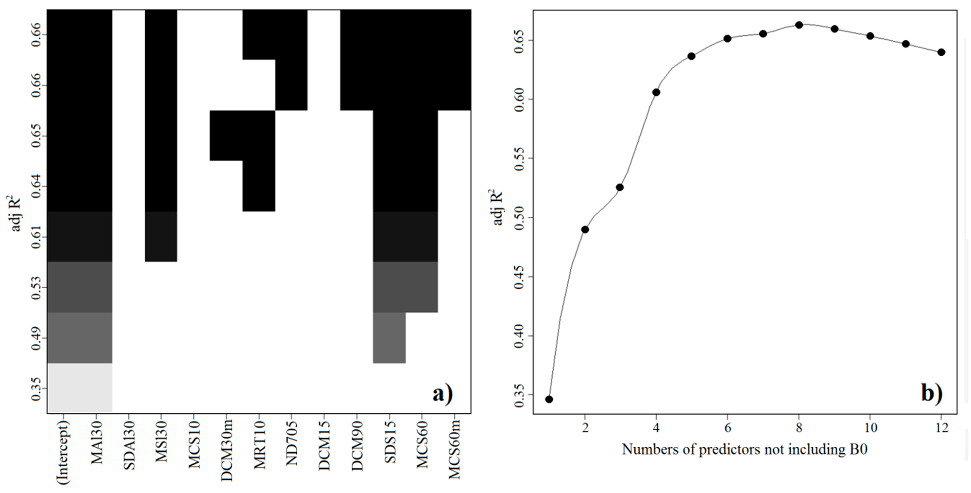
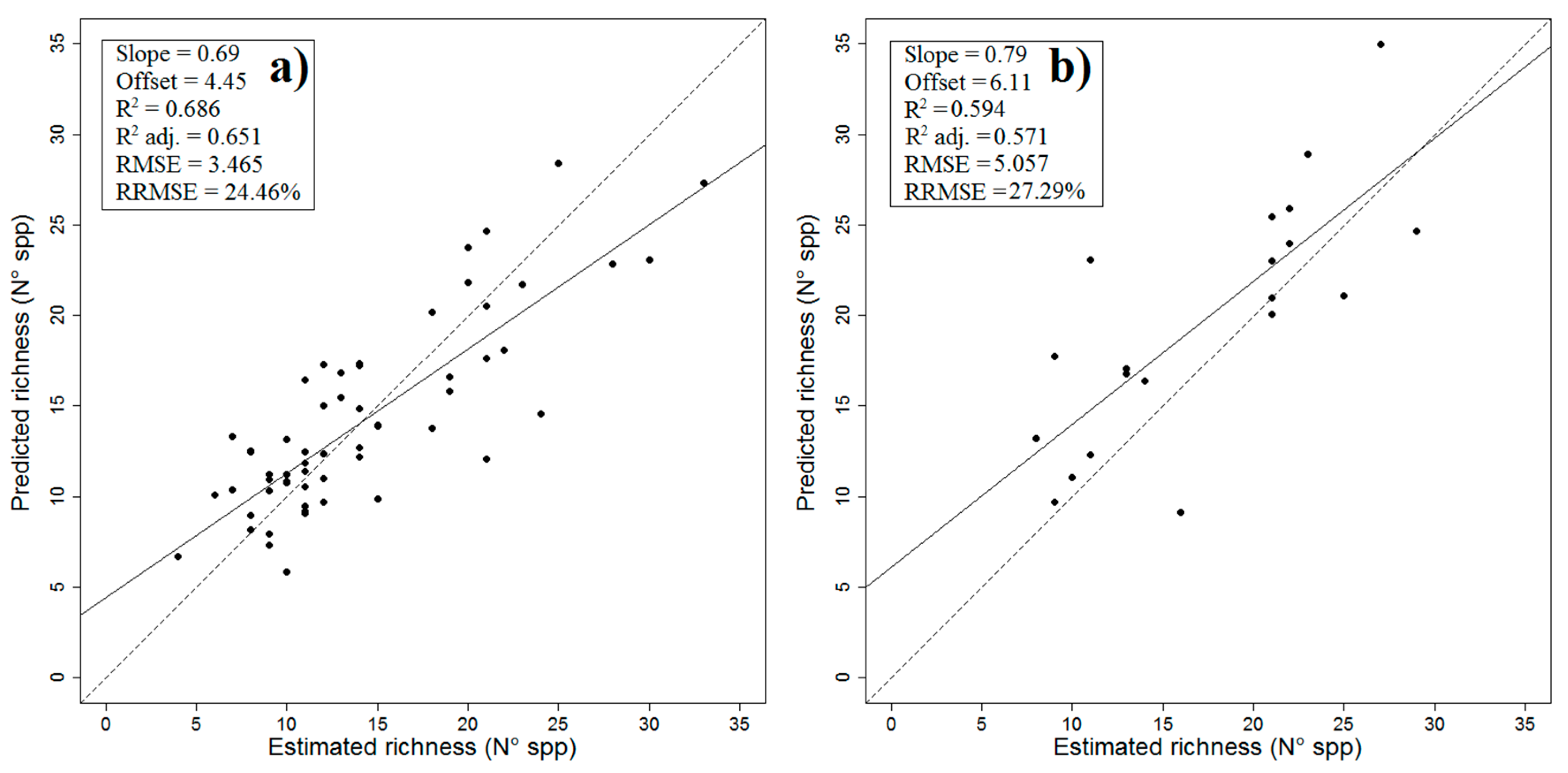
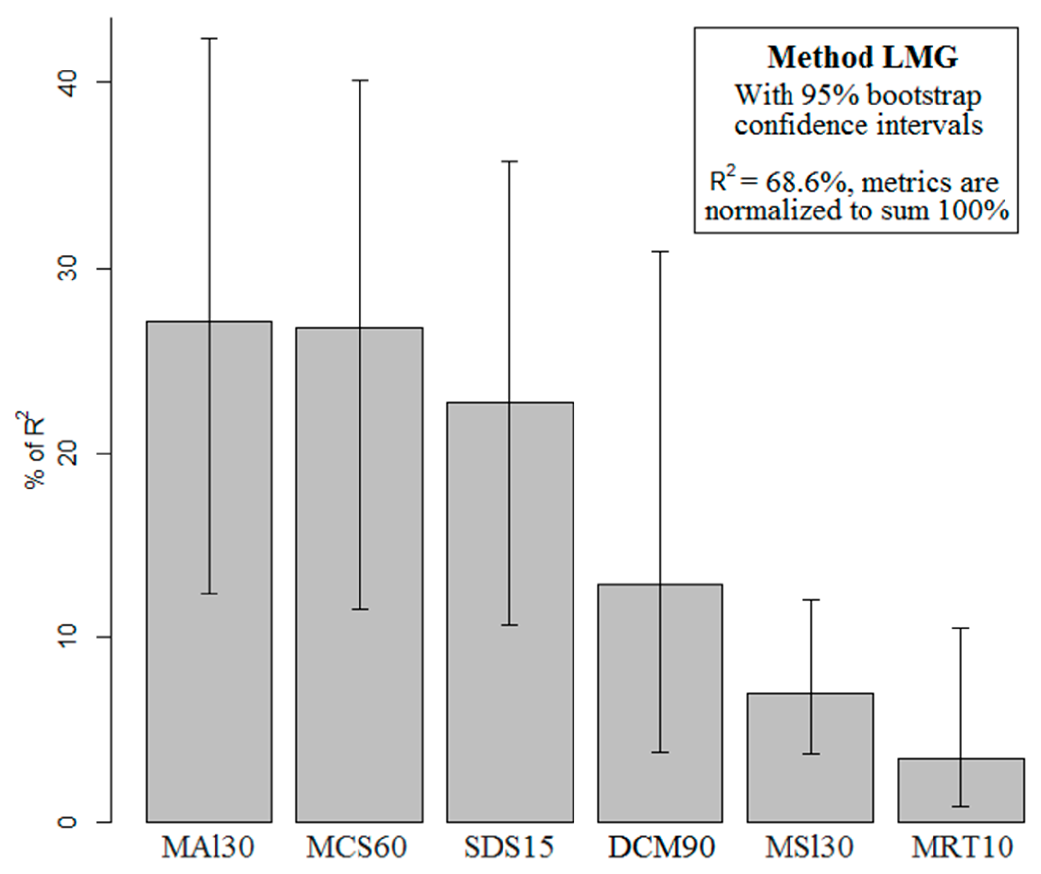
2.1. Final Predictive Model

The exploratory step was performed with the RF classifier to select 12 major predictors (Figure 1). At this point, most of the selected predictors were provided by the LiDAR information, omitting the hyperspectral information except for the Normalized Difference Vegetation Index (ND705) (Figure 2). The 11 LiDAR selected predictors were nine topographical variables: mean altitude (DTM10), standard deviation of altitude (SDAl30), mean slope (MSl30), median catchment slope (MCS60m), mean catchment slope (MCS60), MrRTF (multiresolution index of the ridge top flatness) (MRT10), standard deviation of slope (SDS15), and two structural predictors: mean digital crown model (DCM15), median digital crown model (DCM90). The selected predictors were strongly associated with the results of Corvalan et al. [40], where altitude and the landform indexes were used as variables to explain the presence, abundance, and associativity of several tree species in the same area.
Y   ^ =   19.4     0.01 MAL 30     0.19 MSL 30   +   3.65 MRT 10   + 1.25 SDS 15   +   42.49 MCS 60     0.38 DCM 90
Figure 1. Data processing flow chart to obtain the predictive model of plant richness.
Remotesensing 07 02692 g001
The 12 predictors defined by the exploratory approach were used in a best subset regression approach to define the optimal number of predictors with the highest adjustment. The analysis indicated eight variables to obtain the maximum adjusted R2 (Figure 2a,b), but after including all of these variables in a multiple linear regression, some of the assumptions were not met. We excluded those predictors that affected the statistical assumptions to avoid affecting the predictive power of the model. Six variables were ultimately obtained: MAl30, SDS15, MCS60, MSl30, MRT10, and DCM90 as described in Equation (1). Thus, only LiDAR information was considered with one structural and five topographical predictors. These results can be explained by the fact that different spatial resolutions were considered, including airborne and spaceborne data. Camathias et al. [41] established that an increase in the spatial resolution of remote sensing can improve the accuracy of models to obtain richness prediction.
Figure 2. (a) Table of models showing which variables are in each model. The models are ordered by the adjusted R2. MAl30: mean altitude (30 m); SDAl30: standard deviation of altitude (30 m); MSl30: mean slope (30 m); MCS10: mean catchment slope (10 m); MRT10: MrRTF (10 m); ND705: NDVI (30 m); DCM15 digital crown model (15 m); DCM90: median digital crown model (90 m); SDS15: standard deviation of the slope (15 m); MCS60: mean catchment slope (60 m); MMCS60: median catchment slope (60 m). Note that the axis is not quantitative but ordered. The darkness of the shading simply represents the ordering of the adjusted R2 values (b) Plot of the number of predictors that maximize the adjusted R2.
Remotesensing 07 02692 g002
The final model had a residual mean standard error (RMSE) of 3.69 species, with 53 degrees of freedom and an adjusted determination coefficient (R2) of 0.651 (Figure 3a). There was a slight tendency to overestimate in areas with low richness and to underestimate slightly in zones with high richness. The validation set provided similar results but with lower, significant accuracy (Figure 3b), and demonstrated the robustness of the present approach. These results are similar to those obtained by Carlson et al. [23], which were evaluated for an insular tropical forest using only hyperspectral information, and to those of Hernández–Stefanoni et al. [42], also for a tropical forest using only multispectral information. Other studies obtained better biodiversity predictions (R2 > 0.73) under tropical conditions by considering the Shannon index as a dependent variable [43,44]. Under Mediterranean conditions, similar predictions to those obtained in our study were obtained by Simonson et al. [45] and Bacaro et al. [46] by using the Shannon index and richness, respectively. In another context, Camathias et al. [41] obtained lower richness prediction accuracies (R2 = 0.53) for the whole of Switzerland, which is mainly composed of alpine ecosystems (60%). These examples show the predictive differences of these models depending on the ecosystem type. In this sense, Camathias et al. [41] also mentioned that the importance of a remotely sensed variable is strongly dependent on the biogeographic context, which highlights the need to perform studies of poorly investigated ecosystems such as complex Mediterranean areas.
Figure 3. (a) Statistics of the estimated richness vs. predicted richness obtained in the model construction (60 clusters); (b) Statistics of the estimated richness vs. predicted richness obtained in the independent validation set (20 clusters).
Remotesensing 07 02692 g003
Table 1. Evaluation of the assumptions of the multiple linear regression and validation regression analysis. *: Assumptions acceptable (p-value > 0.05); : Assumptions acceptable (√VIF < 2); ¥: Assumptions acceptable (p-value < 0.05); §: Closest Cluster to be outlier; MCS60: Mean Catchment Slope (60 m); DCM90: Median Digital Crown Model (90 m); MRT10: MrRTF (10 m); SDS15: Standard Deviation of the slope (15 m); MAl30: Mean Altitude (30 m); MSl30: Mean Slope (30 m). Spatial autocorrelation was evaluated over residuals with the Moran test.
Linear Model AssumptionsValuep-value
Global Stat4.2420.3742 *
Skewness3.3890.0657 *
Kurtosis0.0010.9728 *
Nonlinear link function0.6350.4257 *
Heteroscedasticity0.2180.6407 *
Outlier EvaluationClusterp-valueBonfer. p
Bonferroni test25 §0.0068 ¥0.4091
Residuals NormalityWp-value
Shapiro–Wilk normality test0.96980.1435 *
Co-linearity EvaluationMCS60DCM90MRT10SDS15MAl30MSl30
Variance Inflex Factors (VIF)2.935 1.302 1.394 1.426 1.306 2.69
Validation regression analysisAdj R2p-valueRMSE
0.57146 × 10⁻⁵ ¥5.057
Autocorrelation TestIndexExpect.z-scorep-valuepattern
Global Moran’s I−0.0851−0.0169−080670.4197 *random
Correlations between the final predictors are worthy of note for being relatively low (R < 0.5) among all variables included in the predictive model except for the slope variables MS130 and MCS60, which were R = 0.78. These correlation results indicate a low repetition or redundancy of information among variables, which was ratified by the co-linearity analysis of the Variance Inflex Factor (VIF) summarized in Table 1. This table also validates the set of assumptions that corroborate the robustness of the proposed multiple regression model. The robust parametric assumption test provided by the model (Table 1) indicates that the inclusion of other, more complex methods such as the generalized linear mixed models (GLMM) or non-parametric approaches such as the RF regression or the generalized additive models (GAM) were not necessary.

2.2. Ecological Implications

In a broad sense, the selected predictors represent the environmental variability in Monte Oscuro, ratifying a positive correlation between environmental heterogeneity and species richness, which has also been found in other studies [16,18,20,35]. The variables derived from LiDAR information were the best estimators of plant diversity (Figure 4), supporting the notion that greater variability in different biotic and abiotic conditions and the larger number of niches these may provide are important factors in the estimation of diversity [46]. Using high spatial resolution LiDAR data, Dufour et al. [18] determined that the heterogeneity they captured affected plant richness patterns on a local scale. This methodological consideration may be relevant if we consider that the forest of Monte Oscuro had a sensitive variation in spatial dynamics, which was favored by the LiDAR pixel with the best resolution. Altitude (MA130) had the greatest relative importance among the variables (Figure 4). The range of elevation in the study was about 700 m, which generates an important gradient of temperature conditions that is a key factor in mountain ecosystems determining different vegetation zones [8]. The same variable proved to be heavily discriminatory in characterizing several tree species in the same area [40]. The importance of this variable is consistent with the results of several studies [19,41,47], where altitude (at different resolutions) is always among the selected variables in predictive models, particularly on the regional scale [46]. Other predictors with significant relative importance were those related to the slope (SDS15 and MS130), an important source of environmental variation for Monte Oscuro, as has been reported for other ecosystems [19,20,37]. Predictors directly derived from this variable have been reported as second in importance on the local [46] and regional scale [19] for different ecosystems. With respect to the landform indexes, the MCS60 and MRT10 were also relevant; these are directly related to geomorphology and, thus, to accumulation processes linked to soil formation [48]. These variables appear to be indicating environmental variability related to edaphic conditions, which has been reported in a community composition study [49]. Indeed, these variables may have a direct relation to soil particle size. Therefore, water availability to root systems and, particularly, soil moisture has been shown to be one of the most important structuring factors for vegetation communities at the local spatial scale [50,51]. The distribution of nutrients could also be affected by the topographical conditions. Indeed, given the greater homogeneity of chemical, physical and biological plant growth factors, a smooth terrain profile should provide fewer niches than a steeper (and presumably uneven) profile, and thus have lower species richness as well [52]. MCS60 represents an integrated slope averaging a bigger area and is, therefore, an indicator of the landscape variability on a larger scale [49]. In this way, the landforms have already been highlighted as relevant indicators able to explain the spatial pattern of species distribution [53].
Figure 4. Relative importance of the variables of the model of vascular plant richness based on the percentage of the representation of R2 obtained by the LMG method [54]
Remotesensing 07 02692 g004
The digital crown height model (DCM90), which represents the only forest structural variable, was also of considerable relative importance in the predictive model, which was also found by Dufour et al. [18], Bässler et al. [47], and Féret & Asner [43]. In this sense, the structural heterogeneity could be one of the main drivers of variation in species richness due to the patterns formed in the gap-to-understory environments [18]. This kind of variable has also been used as an indicator of the vertical structure of vegetation for biodiversity studies related to other taxonomic groups such as mammals, reptiles, and insects [55].
The forest ecosystems of the Andes foothills of central Chile have a particular vertical and horizontal complexity in addition to their location in a topographically complex area, which limits studies related to remote sensing and biodiversity. The total species richness recorded in the 80 sample plots was 126 species; this demonstrates the important diversity of this area, as also indicated by other authors [6]. Studies that have successfully estimated diversity have mostly concentrated on relatively flat areas [16,25,44,56]. Some studies have focused on altitudinal range similar to Monte Oscuro but none of them on the same local scale [19,47]. Over complex terrain areas, the inclusion of high-resolution topographical and structural variables derived from a LiDAR point cloud may represent a relevant contribution to the estimation of diversity, as demonstrated in several studies [20,41,46,47] including this one. Because of the singular conditions of the complex native forest of the Andes foothills of central Chile, it is expected that more robust results will be obtained by modeling plant diversity using the differentiation of different plant strata (tree, shrub, and herb canopies separately), due to the high capacity of LiDAR to capture the variability of these strata, as shown in other studies [26,57].
The Monte Oscuro site has considerable heterogeneity in topography and geomorphology, which was recorded as an important variation in the magnitudes of the topographical and geomorphological variables estimated. The study zone was relatively homogeneous in terms of the radiation received; climatic and lighting variables such as total insolation were also discarded during the exploratory analysis. The main reason could be that the site is mostly a southern exposure, indicating a homogeneous and similar condition in terms of the radiation received. In studies on the local scale, the variation in climatic and lighting conditions seems less important to explain the biodiversity prediction than when regional scales were considered [19,41,46].
With respect to the hyperspectral information, even if one of the spectral predictors was selected in the final subset of 12 variables, a possible explanation for the low predictive power of the hyperspectral-derived predictors could be the local scale of the study area and the spatial resolution of the spaceborne sensor. The results of this research did not allow us to confirm the spectral variation hypothesis on a local scale, even though Oldeland et al. [56] suggested that the use of hyperspectral information should improve monitoring of species diversity. In this light, recent studies [43,44] have proven that the hyperspectral information from airborne sensors can significantly enhance the predictive power of models not only because of the spectral information but also because of the improvement provided by the spatial resolution [24,26,41,58,59]. Another relevant source of information could be an analysis of seasonal and annual variability that can provide an additional element in estimating biodiversity [24], particularly in deciduous forests like Monte Oscuro. Another possible way to improve the hyperspectral contribution could be a more refined methodology to optimize the information contained in the hyperspectral image; this might have contributed better to managing the complexity of the multidimensional structure which hyperspectral data possess [33]. The recommendation of Ginzburg & Jensen [60] and Rocchini et al. [16] to incorporate more elaborate methods to explain the complexity that characterizes plant diversity explains, to a certain degree, why no hyperspectral variables were in the final predictive model. Kalacska et al. [25] obtained a significant prediction of diversity using images from the same Hyperion sensor but utilizing a more complex methodology than the one used in this study (Wavelet transformation with temporal-seasonal analysis) and in a dry tropical forest ecosystem. Parviainen et al. [19], using GAMs, improved the explanatory power of remote sensing variables in assessing biodiversity and species distribution.

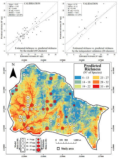
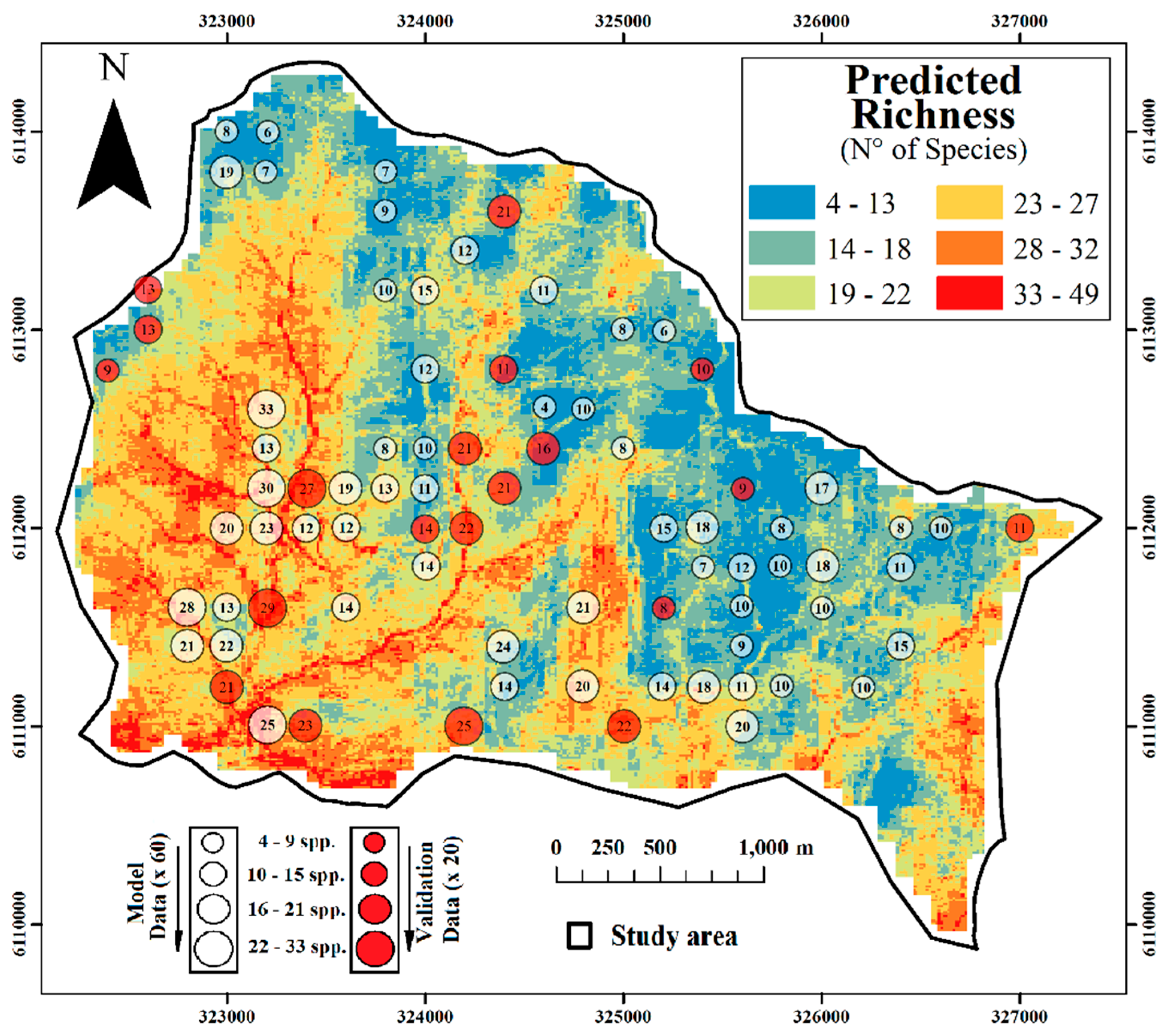
2.3. Spatial Prediction

The spatial prediction of vascular plant richness was depicted as a richness map estimated by applying the coefficients to the variables of the final predictive model (Figure 5).
The highest richness levels were associated with the lowest part of the study area and sections close to the main water courses (Figure 5). Different studies have stated that the spatial distribution of biodiversity is clearly affected by altitude variation, with a negative correlation with richness in different ecosystems [61,62]. The important variability in richness recorded on the plots is also clearly depicted on the map; this varied from 4 to 49 species and is clearly reflected in the colors of the richness map. The main variables selected in the predictive model are associated with elevation as well as with the topographical and geomorphological features of the area, along with the digital crown model that represents crown height. Most of these characteristics represent conditions of environmental variability on a local scale. Comparable results have been reported for regional scales [24,36], showing a variable relative importance depending upon the scale [18]. According to Kolasa & Rollo [63], heterogeneity may be mostly explained by three components: (i) the environmental variability or range in which the different environmental conditions of the site are variable (number of habitat types); (ii) the spatial configuration of the different habitats of the site; and (iii) by the historical variation over time. Monte Oscuro appears to have a large number of niches according to the variation in richness recorded on the plots (Figure 5), whereas its spatial configuration was clearly influenced by environmental conditions linked to the above-mentioned environmental conditions. Greater richness values were associated with lower zones with favorable micro-meteorological conditions mostly related to higher temperatures, along with a theoretically adequate water supply with micro-topographical conditions of heterogeneity that can provide different conditions for plant establishment. This area has at least five months of the year without precipitation, which produces a water deficit sufficient to affect the plant composition of the forest. It should also be remembered that this precise area is located in a transitional vegetation zone where sclerophyll forest coexists with the Valdivian forest evergreen species in a matrix of Nothofagus obliqua [8], which significantly increases the richness. Finally, it should be noted that Monte Oscuro is a secondary forest. Although there is currently little or no intervention, in the past, the intervention was enough to influence forest structure, affecting the current richness.
Figure 5. Spatialization of the predictive model of plant vascular richness. White circles depicted the richness value of the sampling plot used for the model construction. Red circles depicted the richness values of the sampling plots used for validation purposes.
Remotesensing 07 02692 g005
Lastly, it is also notable that resampling the predictor variables at differing spatial resolutions that more adequately reflect the field situation improved the prediction. The selection and concern of the spatial resolution have relevant implications in ecological studies [49] and within the taxonomical groups considered [55]. The consideration of different grain size of the selected predictors has been used mainly in studies on regional and continental scales [56,64,65,66]. Some of the predictors included in the final model, such as the DCM90 or the MCS60, were aggregated at a coarser resolution from the original data. Similar resampling techniques provided better representativity of the environmental heterogeneity because the spatial grain of predictors strongly affects the ecosystem structural properties related to remote sensing, and this partially determines certain patterns of species clustering in communities [49].

3. Experimental Section

3.1. Study Area

The study area is located at the Andes foothills of central Chile in the Maule region, province and commune of Curicó at the Monte Oscuro site (35°07ʹ00ʺ S, 70°55ʹ30ʺ W) (Figure 6a). This sector is associated with the sub-Mediterranean temperate bioclimatic zone, with a mean annual precipitation of 1000 mm concentrated between April and October, and mean temperatures ranging from 8 °C in the coldest months (June to August) to 18 °C in the warmest months (December to February). The site has an area of 12.95 km2 and a surface area of 14.50 km2, with a mean altitude of 1075 m.a.s.l. (varying from 650 to 1500 m.a.s.l.) and mostly southern exposure, presenting a very complex and heterogeneous topography with high microsite variations. The vegetation is a secondary deciduous forest dominated by Nothofagus obliqua (Mirb.) Oerst. mixed with the sclerophyll species Quillaja saponaria Mol., Cryptocarya alba (Molina) Looser, Lithraea caustica (Molina) Hook et Arn., and the Valdivian forest evergreen species Myrceugenia exsucca (DC.) Berg and Podocarpus saligna D. Don, which according to Luebert & Pliscoff [8], corresponds to the “Deciduous Mediterranean Andean forest of Nothofagus obliqua and Austrocedrus chilensis.” In the study area, this formation presents a very dense and tangled understory, with multiple layers (three or more) between the ground and the upper canopy mainly dominated by Nothofagus obliqua.
Figure 6. (a) Location of the study area; (b) Spatial distribution of field samples (model clusters in black and validation clusters in red); (c) Detail of a sampling unit with nested plots.
Remotesensing 07 02692 g006

3.2. Field Data

This study used vascular plant richness as the only variable to be predicted, as a surrogate of total biodiversity. This taxonomic group was chosen due to its clear dominance in the forests of the study area and because it is essential in the trophic network of almost all other land animals and plants [5]. The model construction sampling was performed between 7 and 11 January 2013 (20 plots) and between 14 and 22 March 2013 (40 plots). In these ecosystems, most of the flora is present during the whole summer period, particularly the vascular plant richness. In terms of annual vegetation, even if some of this was not present in its active state during March, we were careful to identify the remaining dry parts of leaves, fruit, and flowers. A systematic sampling design of 60 square nested plots [28,67] separated by 200 m was considered. Each sampling point was determined randomly inside the 200 m grid design by discarding those plots with slopes greater than 45° and with strong accessibility problems due mainly to tangled vegetation (Figure 6b).
Sampling plots were constructed to capture floristic information from three types of plant cover: trees, shrubs, and herbs. We established six nested subplots on each plot, the largest of which was 225 m2 (15 m × 15 m), with its vertices in the four cardinal points of north, south, east and west. In the largest plots, we identified the species of all woody individuals taller than 2 m (defined as trees). Two subplots of 25 m2 (5 m × 5 m) were located in the northern and southern corners of the 225 m2 plot, in which we identified the species of all woody individuals under 2 m (defined as shrubs). Within each 25 m2 subplot, we established sub-subplots of 1 m2, in the northern corner of the northern subplot and the southern corner of the southern subplot. We also included a third 1 m2 sub-subplot in the center of the 225 m2 plot, equidistant between the other two (Figure 6c). In each of the three 1 m2 plots, we identified the species of all non-woody individuals (defined as herbs). The information from the 1 m2 and 25 m2 plots was expanded linearly to their respective 225 m2 plots, thereby obtaining the total richness of vascular species for each group (conglomerate) of plots [40]. The establishment of the field sampling area was made based on a visual inspection of a larger area, making sure that the selected area was representative of the variability present within the Hyperion pixel. If this is not met, the center of the plot was moved until the 225 m2 sampling area covered a representative area of the 900 m2 Hyperion pixel.
Using the same sampling methodology, a validation floristic survey was performed between 20 and 27 January 2014 (20 plots) with 20 independent sampling points (Figure 6b).

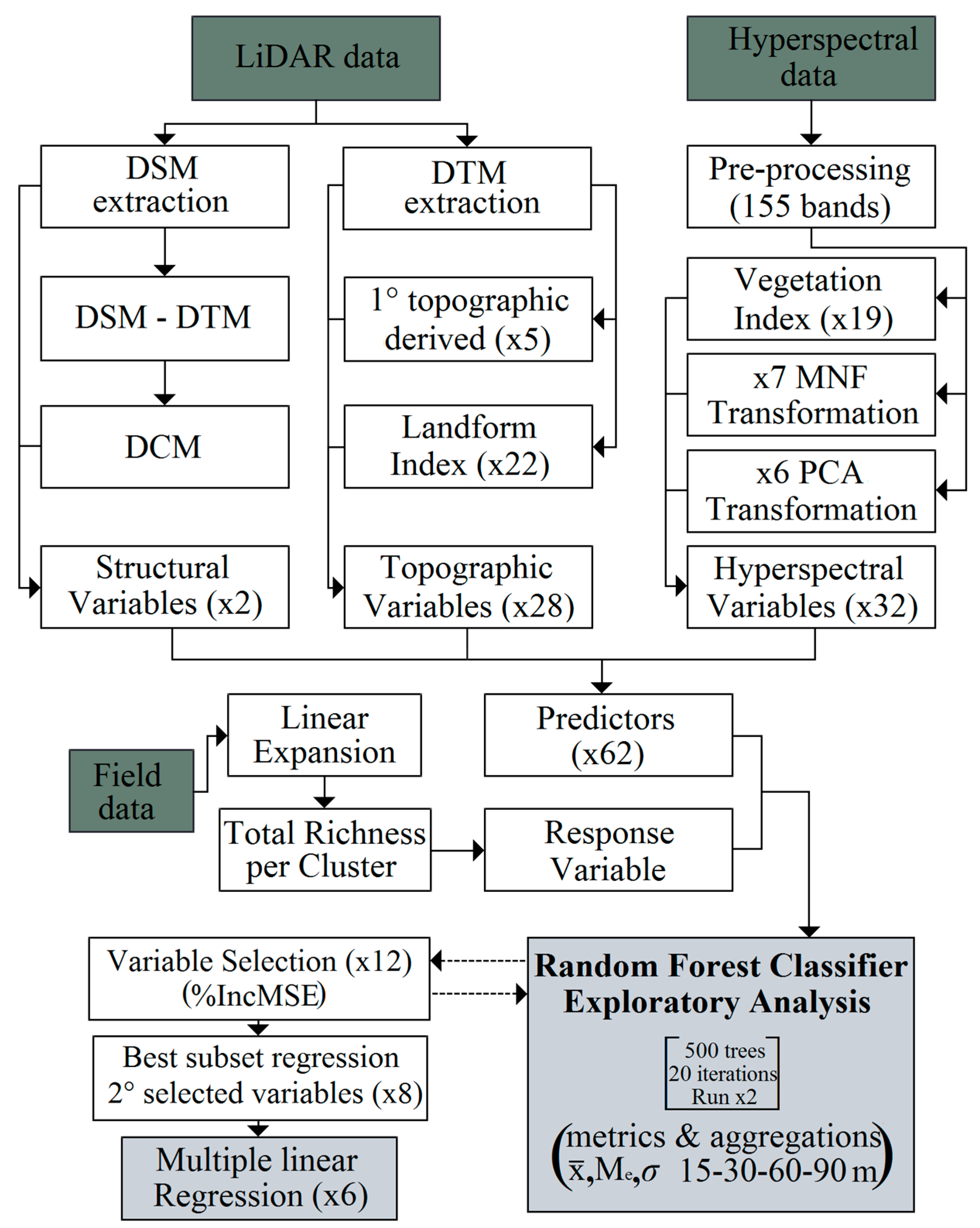
3.3. Remote Sensing Data

3.3.1. Hyperspectral Information

The hyperspectral variables were derived from a Hyperion dataset at processing level L1R from the EO-1 satellite, acquired on 25 February 2011 (ID: EO1H2330842011056110KF), which had a swath width of 7.5 km, a spatial resolution of 30 m and a spectral resolution of 242 bands with a 10 nm spectral width, which ranged from a 400 to a 2500 nm wavelength [68].
Table 2. Summary of predictor variables (hyperspectral and Light Detection and Ranging (LiDAR)) used to generate the predictive model of richness.
PredictorsTypeNameReference
Hyperion Hyperspectral Image 155 reflectance bandsVegetation Index (non–photosynthetic vegetation)Cellulose absorption index (CAI)[75]
Plant Senescence Reflectance Index (PSRI)[76]
Vegetation Index (live vegetation, vigor, greenness)Enhanced vegetation index (EVI)[77]
Modified red edge Simple Ratio Index (mSR705 )[78]
Canopy Single Ratio (SRcanopy)[79]
Single Ratio (SR705)[79]
Simple Ratio Vogelmann index (SRv)[80]
Modified Normalized Difference Vegetation Index (mND705)[79]
Canopy Normalized Difference Vegetation Index (NDcanopy)[79]
Normalized Difference Vegetation Index (ND705)[79]
Modified Single Ratio (MSR)[81]
Ratio TCARI/OSAVI[82]
Vegetation Index (canopy structural water)Moisture Stress Index (MSI )[83]
Normalized Difference Infrared Index (NDII)[84]
Normalized Difference Water Index (NDWI )[85]
Water Band Index (WBI)[86]
Water Index (WI1180 )[87]
Vegetation Index (photosynthetic activity)Photochemical Reflectance Index (PRI)[88]
Total Chlorophyll Concentration[89]
Transform (Processing of dimensionality reduction)Forward Principal component analysis (PCA) (first 6 components)[73]
Minimun Noise Fraction (MNF) (first 7 components)[74]
Light Detection and Ranging (LiDAR) 3D Point Cloud and derived Digital Terrain Model (DTM)DTM10Altitude
First topographic derived (from DTM)Slope[90]
Aspect[90]
Curvature[90]
Plan Curvature[90]
Profile Curvature[90]
Landform variable (Hydrology from DTM)Catchment Area[91]
Catchment Height[91]
Catchment Slope[91]
Flow Path Length[92]
Valley Depth[93]
Landform variable (Topo–hydrology from DTM)SAGA Wetness Index[94]
Slope Length[93]
Stream Power Index[95]
Topographic Wetness Index (TWI)[96]
TCI Low[97]
LS–Factor[96]
Landform variable (Topo–morphometry from DTM)Topographic Position Index (TPI)[98]
Morphometric Protection Index[99]
Terrain Ruggedness Index (TRI)[100]
Multi–resolution Index of Valley Bottom Flatness (MrVBF)[48]
Multi–resolution Index of Ridge Top Flatness (MrRTF)[48]
Convergence Index[93]
Vector Ruggedness Measure (VRM)[101]
Climate and Lighting (from DTM)Diurnal Anisotropic Heating[93]
Total Insolation[102]
Topographic Positive Openness[99]
Analytical Hillshading[103]
Structural variables DSM10
DCM10
The pre-processing and image corrections were performed with the ENVI 5.0 software, using the methodological steps developed by Datt et al. [69], including the extraction of the spectral subset (excluding uncalibrated bands with spectral superposition and those with multiple anomalous values, leaving 155 bands) and the spatial subset of the study area, finally obtaining reflectance values using the FLAASH atmospheric correction [70]. The scene was also georeferenced to the WGS-84 geodetic datum using 40 control points and a total RMS error of ± 0.1 pixels with the help of an Orthophoto obtained during the LiDAR flight (0.5 m spatial resolution) plus a Landsat 7 ETM+ image (30 m spatial resolution) from 26 February 2011.
From the preprocessed scene, 19 vegetation indexes widely used in the literature associated with hyperspectral remote sensing [71,72] and the first components of two transformations to reduce the noise and dimensionality of the band set—a forward principal components analysis (PCA) [73] and a minimum noise fraction (MNF) [74]—were calculated by selecting the components to be used based on the interpretation of the PCA and MNF eigenvalue plot and visual inspection of the bands. The 32 hyperspectral variables used in the statistical analyses are summarized in Table 2.

3.3.2. LiDAR

The LiDAR point cloud was acquired in February 2011 using a Harrier 54/G4Dual System sensor mounted on a Piper PA-24 Comanche airplane, achieving an average point cloud density of 4.64 points/m2. The pulse and scanning frequencies were 100 kHz and 100 Hz, respectively, with a field vision angle of approximately 22.5° and a laser pulse wavelength of 1550 nm. Using the “lasground.exe” tool of LAStools software [104], the point cloud was classified as ground and no ground returns, subsequently obtaining from these a digital terrain model (DTM) and digital surface model (DSM) respectively with the “las2dem.exe” tool, both with a spatial resolution of 10 m. We then calculated a digital crown height model (DCM) by the difference between the DSM and the DTM.
We then used the SAGA GIS software [93] to calculate, based on the DTM, first-order topographical variables, landform variables associated with morphometrics, hydrology and topography, and variables associated with the illumination of the study area: 28 variables we called topographic variables. DSM10 and DCM10 were used as structural variables [105]. These 30 variables acquired from LiDAR are summarized in Table 2.

3.4. Statistical Analysis and Spatialization

A total of 62 variables were used for the predictive model of richness, which was performed with the R-project software [106]. The first stage occupied the Random Forest (RF) package [107] in regression mode as an exploratory analysis to give priority to and select the relevant variables in the prediction of richness. We used RF because of its improvements over other tree classification techniques [59]. Its ability to construct hundreds of decision tree models using random subsets of the variables, in addition to its internal cross-validation and bootstrap aggregation (bagging) [108], make it a powerful tool for variable selection.
Twenty replicas of the classifier using 500 decision trees each time were run to choose the most important and stable variables based on the percentage increase of the mean square error (%IncMSE), which was generated when they were not selected. To improve the prediction and include the different spatial resolution of the variables [42,109], the grain size of these pre-selected variables was modified by aggregating the pixels at different spatial resolutions (15, 30, 60 and 90 m) with different grouping criteria (mean, median, and standard deviation of the neighboring pixels). The aggregate function of the Spatial Analyst toolbox of ArcGIS 10.1 was used to obtain the different grain size.
Secondly, these pre-selected variables, some metrics, and their aggregations at different resolutions were used as input for a new run of the RF model for selecting the best predictive variables, using the same parameters as in the first stage. With this approach, 12 variables were selected according to the most common selection after 20 iterations. After this coarse variable selection, a best subset regression technique was applied to the 12 pre-selected variables according to the “leaps” packages [110]. According to this criterion, a multiple linear regression model was obtained by optimizing the best quantity and types of predictors. Finally, we applied the coefficients obtained from the multiple linear regression to each selected predictor and thus produced a spatial interpolation of the richness.
To evaluate the robustness of the final multiple linear model generated, we used the “gvlma” package of R [111], based on a single global test and on specific directional tests to measure the asymmetry, kurtosis, a non-linear link function, and heteroscedasticity, using a significance level of 0.05. The normality of the multiple regression residuals was also verified using the Shapiro-Wilk test from the R “stats” package [112], possible outliers with the Bonferroni test and co-linearity using the variance inflex factor (VIF), both using the car-package R function [113]. The relative importance of the variables of the final predictive model (R2 and confidence intervals) was then evaluated using the Lindeman, Merenda and Gold method (LMG) of the “relaimpo” package of R [54]. The spatial autocorrelation of model residuals was evaluated using Moran’s I test available in the ArcMAP 10.1 software [114]. Finally, a regress analysis between validation points and the corresponding modeled values was performed in R, obtaining a validated R2 and RMSE.

4. Conclusions

The main objective was to predict and spatialize the vascular plant richness (alpha diversity) present in a secondary mixed deciduous forest of the Andes foothills of the Maule region, Chile. This was achieved using only structural variables derived from airborne LiDAR data, discarding the spaceborne hyperspectral information that, despite being significant, showed a lower predictive power. The information on altitude represented by DTM, the standard deviation of the slope, and the catchment slope were the variables that contributed most to predicting the richness of the plots (all derived from LiDAR).
On the local scale utilized, the contribution of LiDAR data was significant in the development of the model selections, whereas the hyperspectral information did not provide a significant contribution to the prediction of plant richness. The inclusion of aggregated topographical information proved to be a relevant predictor in the final model. Other processing methodologies applied to a larger geographical expanse might generate better results.
This study demonstrates that the plant species richness of Mediterranean deciduous forests and their spatial heterogeneity can be modeled and predicted with sufficient precision to be used in management and conservation plans, highlighting the great potential of this type of focus for evaluating and monitoring biodiversity.
There are opportunities to improve the methodological approaches and review the use of other predictive variables (acquired both from LiDAR and hyperspectral information), or include an analysis with spectral images of finer resolution.

Acknowledgments

This work was partially funded by CONICYT project, Integration of Advanced Human Capital into the Academy, code 791100013 and by the U-INICIA VID 2012, code 1/0612, University of Chile.
We are grateful to Luis Faúndez, botanist of the Faculty of Agronomic Sciences, University of Chile, for his assistance in the identification of plant specimens collected during the research.

Author Contributions

Andres Ceballos collected field data, processed and analyzed the data, and wrote the manuscript. Jaime Hernandez helped in the design of the experiment, discussed the results, and contributed to the writing of the manuscript. Patricio Corvalán helped in the design of the experiment, discussed the results, and contributed to the writing of the manuscript. Mauricio Galleguillos collected field data, processed and analyzed the data, contributed to the writing of the manuscript, and discussed the result and statistical analysis.

Conflicts of Interest

The authors declare no conflict of interest.

References

  1. Duffy, J.E. Why biodiversity is important to the functioning of real-world ecosystems? Front. Ecol. Environ. 2006, 7, 437–444. [Google Scholar] [CrossRef]
  2. Balvanera, P.; Pfisterer, A.B.; Buchmann, N.; He, J.S.; Nakashizuka, T.; Raffaelli, D.; Schmid, B. Quantifying the evidence for biodiversity effects on ecosystem functioning and services. Ecol. Lett. 2006, 9, 1146–1156. [Google Scholar] [CrossRef] [PubMed] [Green Version]
  3. Carpenter, S.R.; Bennett, E.M.; Peterson, G.D. Scenarios for Ecosystem Services: An Overview. Available online: http://www.uvm.edu/giee/pubpdfs/Carpenter_2006_Ecology_and_Society.pdf (accessed on 1 September 2014).
  4. Díaz, S.; Fargione, J.; Chapin, F.S.; Tilman, D. Biodiversity loss threatens human well-being. PLoS Biol. 2006, 4, 1300–1305. [Google Scholar] [CrossRef]
  5. Myers, N.; Mittermeler, R.A.; Mittermeler, C.G.; da Fonseca, G.A.B.; Kent, J. Biodiversity hotspots for conservation priorities. Nature 2000, 403, 853–858. [Google Scholar] [CrossRef] [PubMed]
  6. Squeo, F.A.; Estévez, R.A.; Stolla, A.; Gaymerb, C.F.; Leteliera, L.; Sierralta, L. Towards the creation of an integrated system of protected areas in Chile: Achievements and challenges. Plant Ecol. Divers. 2012, 1, 1–11. [Google Scholar]
  7. Estrategia Y Plan De Acción Para La Biodiversidad En La VII Región Del Maule. Available online: www.sinia.cl/1292/articles-37025_pdf_maule.pdf (accessed on 2 March 2015).
  8. Luebert, F.; Pliscoff, P. Sinopsis Bioclimática y Vegetacional de Chile; Editorial Universitaria: Santiago, Chile, 1999. [Google Scholar]
  9. Altamirano, A.; Lara, A. Deforestation in temperate ecosystems of pre-Andean range of south-central Chile. Bosque 2010, 31, 53–64. [Google Scholar] [CrossRef]
  10. Echeverria, C.; Coomesa, D.; Salas, J.; Rey–Benayas, J.M.; Lara, A.; Newtone, A. Rapid deforestation and fragmentation of Chilean Temperate Forests. Biol. Conserv. 2006, 130, 481–494. [Google Scholar] [CrossRef]
  11. González, M.E.; Lara, A.; Urrutia, R.; Bosnich, J. Climatic change and its potential impact on forest fire occurrence in south-central Chile (33°–42° S). Bosque 2011, 32, 215–219. [Google Scholar] [CrossRef]
  12. Bellard, C.; Bertelsmeier, C.; Leadley, P.; Thuiller, W.; Courchamp, F. Impacts of climate change on the future of biodiversity. Ecol. Lett. 2012, 15, 365–377. [Google Scholar] [CrossRef]
  13. Thomas, C.D.; Cameron, A.; Green, R.E.; Bakkenes, M.; Beaumont, L.J.; Collingham, Y.C.; Erasmus, B.F.N.; de Siqueira, M.F.; Grainger, A.; Hannah, L.; et al. Extinction risk from climate change. Nature 2004, 427, 145–148. [Google Scholar] [CrossRef] [PubMed] [Green Version]
  14. Armesto, J.J.; Rozzi, R.; Smith-Ramirez, C.; Arroyo, M.T.K. Conservation targets in South American temperate forests. Science 1998, 282, 1271–1272. [Google Scholar] [CrossRef]
  15. Ceballos, G.; Vale, M.M.; Bonacic, C.; Calvo-Alvarado, J.; List, R.; Bynum, N.; Medellín, R.A.; Simonetti, J.A.; Rodríguez, J.P. Conservation challenges for the Austral and Neotropical America section. Conserv. Biol. 2009, 23, 811–817. [Google Scholar] [CrossRef] [PubMed]
  16. Rocchini, D.; Balkenhol, N.; Carter, G.A.; Foody, G.M.; Gillespie, T.W.; He, K.S.; Kark, S.; Levin, N.; Lucas, K.; Luoto, K.; et al. Remotely sensed spectral heterogeneity as a proxy of species diversity: Recent advances and open challenges. Ecol. Inf. 2010, 5, 318–329. [Google Scholar] [CrossRef]
  17. Turner, W.; Spector, S.; Gardiner, N.; Fladeland, M.; Sterling, E.; Steininger, M. Remote sensing for biodiversity science and conservation. Trends Ecol. Evol. 2003, 18, 306–314. [Google Scholar] [CrossRef]
  18. Dufour, A.; Gadallah, F.; Wagner, H.H.; Guisan, A.; Buttler, A. Plant species richness and environmental heterogeneity in a mountain landscape: effects of variability and spatial configuration. Ecography 2006, 29, 573–584. [Google Scholar] [CrossRef]
  19. Parviainen, M.; Zimmermann, N.E.; Heikkinen, R.K.; Luoto, M. Using unclassified continuous remote sensing data to improve distribution models of red-listed plant species. Biodivers. Conserv. 2013, 22. [Google Scholar] [CrossRef]
  20. Bergen, K.M.; Goetz, S.J.; Dubayah, R.O.; Henebry, G.M.; Hunsaker, C.T.; Imhoff, M.L.; Nelson, R.F.; Parker, G.G.; Radeloff, V.C. Remote sensing of vegetation 3-D structure for biodiversity and habitat: Review and implications for Lidar and radar spaceborne missions. J. Geophys. Res. 2009, 114. [Google Scholar] [CrossRef]
  21. Gaston, K.J. Global patterns in biodiversity. Nature 2000, 405, 220–227. [Google Scholar] [CrossRef] [PubMed]
  22. Pacini, A.; Mazzoleni, S.; Battisti, C.; Ricotta, C. More rich means more diverse: Extending the “environmental heterogeneity hypothesis” to taxonomic diversity. Ecol. Indic. 2009, 9, 1271–1274. [Google Scholar] [CrossRef]
  23. Carlson, K.; Asner, G.; Hughes, R.; Ostertag, R.; Martin, R. Hyperspectral remote sensing of canopy biodiversity in Hawaiian lowland rainforests. Ecosystems 2007, 10, 536–549. [Google Scholar] [CrossRef]
  24. Ewers, R.M.; Didham, R.K.; Wratten, S.D.D.; Tylianakis, J.M. Remotely sensed landscape heterogeneity as a rapid tool for assessing local biodiversity value in a highly modified New Zealand landscape. Biodivers. Conserv. 2005, 14, 1469–1485. [Google Scholar] [CrossRef]
  25. Kalacska, M.; Sanchez-Azofeifa, G.A.; Rivard, B.; Caelli, T.; White, H.P.; Calvo-Alvarado, J.C. Ecological fingerprinting of ecosystem succession: estimating secondary tropical dry forest structure and diversity using imaging spectroscopy. Remote Sens. Environ. 2007, 108, 82–96. [Google Scholar] [CrossRef]
  26. Leutner, B.; Reineking, B.; Müller, J.; Bachmann, M.; Beierkuhnlein, C.; Dech, S.; Wegmann, M. Modelling forest α-diversity and floristic composition—On the added value of LiDAR plus hyperspectral remote sensing. Remote Sens. 2012, 4, 2818–2845. [Google Scholar] [CrossRef]
  27. White, J.C.; Gómez, C.; Wulder, M.A.; Coops, N.C. Characterizing temperate forest structural and spectral diversity with Hyperion EO-1 data. Remote Sens. Environ. 2010, 114, 1576–1589. [Google Scholar] [CrossRef]
  28. Palmer, M.W.; Earls, P.G.; Hoagland, B.W.; White, P.S.; Wohlgemuth, T. Quantitative tools for perfecting species lists. Environmetrics 2002, 13, 121–137. [Google Scholar] [CrossRef]
  29. Gould, W. Remote sensing of vegetation, plant species richness, and regional biodiversity hotspots. Ecol. Appl. 2000, 10, 1861–1870. [Google Scholar] [CrossRef]
  30. Levin, N.; Shmida, A.; Levanoni, O.; Tamari, H.; Kark, S. Predicting mountain plant richness and rarity from space using satellite-derived vegetation indices. Divers. Distrib. 2007, 13, 692–703. [Google Scholar] [CrossRef]
  31. Waring, R.H.; Coops, N.C.; Fan, W.; Nightingale, J.M. MODIS enhanced vegetation index predicts tree species richness across forested ecoregions in the contiguous USA. Remote Sens. Environ. 2006, 103, 218–226. [Google Scholar] [CrossRef]
  32. Deutschewitz, K.; Lausch, A.; Kühn, I.; Klotz, S. Native and alien plant species richness in relation to spatial heterogeneity on a regional scale in Germany. Glob. Ecol. Biogeogr. 2003, 12, 299–311. [Google Scholar] [CrossRef]
  33. Gamon, J.A. Tropical remote sensing—Opportunities and challenges. In Hyperspectral Remote Sensing of Tropical and Sub–Tropical Forests; Kalacska, M., Sanchez-Azofeifa, A., Eds.; Taylor & Francis Group: New York, NY, USA, 2008. [Google Scholar]
  34. Thenkabail, P.S.; Lyon, J.G.; Huete, A. Advances in hyperspectral remote sensing of vegetation and agricultural croplands. In Hyperspectral Remote Sensing of Vegetation; Thenkabail, P.S., Lyon, J.G., Huete, A., Eds.; Taylor & Francis Group: New York, NY, USA, 2012; pp. 12–14. [Google Scholar]
  35. Dauber, J.; Hirsch, M.; Simmering, D.; Waldhardt, R.; Otte, A.; Wolters, V. Landscape structure as an indicator of biodiversity: matrix effects on species richness. Agric. Ecosyst. Environ. 2003, 98, 321–329. [Google Scholar] [CrossRef]
  36. Wohlgemuth, T.; Nobis, M.P.; Kienast, F.; Plattner, M. Modelling vascular plant diversity at the landscape scale using systematic samples. J. Biogeogr. 2008, 35, 1226–1240. [Google Scholar] [CrossRef]
  37. Lefsky, M.A.; Cohen, W.B.; Harding, D.J.; Parker, G.G.; Acker, S.A.; Gower, S.T. Lidar remote sensing of above-ground biomass in three biomes. Glob. Ecol. Biogeogr. 2002, 11, 393–399. [Google Scholar] [CrossRef]
  38. Dalponte, M.; Bruzzone, L.; Gianelle, D. Fusion of hyperspectral and Lidar remote sensing data for classification of complex forest areas. IEEE Trans. Geosci. Remote Sens. 2008, 46, 1416–1427. [Google Scholar] [CrossRef]
  39. Magurran, A.E. Ecological Diversity and Its Measurement; Princeton University Press: New Jersey, NJ, USA, 1988. [Google Scholar]
  40. Corvalán, P.; Galleguillos, M.; Hernández, J. Presencia, abundancia y asociatividad de Citronella mucronata en bosques secundarios dominados por Nothofagus obliqua de la precordillera de Curicó, región del Maule, Chile. Bosque 2014, 35, 269–278. [Google Scholar]
  41. Camathias, L.; Bergamini, A.; Küchler, M.; Stofer, S.; Baltensweiler, A. High-resolution remote sensing data improves models of species richness. Appl. Veg. Sci. 2013, 16. [Google Scholar] [CrossRef]
  42. Hernández-Stefanoni, J.L.; Gallardo-Cruz, J.A.; Meaveb, J.A.; Rocchini, D.; Bello-Pineda, J.; López-Martíneza, J.O. Modeling α- and β-diversity in a tropical forest from remotely sensed and spatial data. Int. J. Appl. Earth Obs. Geoinf. 2012, 19, 359–368. [Google Scholar] [CrossRef]
  43. Féret, J.B.; Asner, G.P. Mapping tropical forest canopy diversity using high-fidelity imaging spectroscopy. Ecol. Appl. 2014, 24, 1289–1296. [Google Scholar] [CrossRef]
  44. Vaglio, G.L.; Cheung-Wai, J.C.; Chen, Q.; Lindsell, J.A.; Coomes, D.A.; Guerriero, L.; Del Frate, F.; Miglietta, F.; Valentini, R. Biodiversity mapping in a tropical west African forest with airborne hyperspectral data. PloS One 2014, 9. [Google Scholar] [CrossRef] [PubMed]
  45. Simonson, W.D.; Allen, H.D.; Coomes, D.A. Use of an airborne Lidar system to model plant species composition and diversity of mediterranean oak forests. Conserv. Biol. 2012, 26, 840–850. [Google Scholar] [CrossRef] [PubMed]
  46. Bacaro, G.; Rocchini, D.; Bonini, I.; Marignani, M.; Maccherini, S.; Chiarucci, A. The role of regional and local scale predictors for plant species richness in Mediterranean forests. Plant Biosyst. 2008, 142, 630–642. [Google Scholar] [CrossRef]
  47. Bässler, C.; Stadler, J.; Müller, J.; Förster, B.; Göttlein, A.; Brandl, R. LiDAR as a rapid tool to predict forest habitat types in Natura 2000 networks. Biodivers. Conserv. 2011, 20, 465–481. [Google Scholar] [CrossRef]
  48. Gallant, J.C.; Dowling, T.I. A multiresolution index of valley bottom flatness for mapping depositional areas. Water Resour. Res. 2003, 39. [Google Scholar] [CrossRef]
  49. Yuan, Z.; Gazol, A.; Wang, X.; Lin, F.; Ye, J.; Bai, X.; Li, B.; Hao, Z. Scale specific determinants of tree diversity in an old growth temperate forest in China. Basic Appl. Ecol. 2011, 12, 488–495. [Google Scholar] [CrossRef]
  50. Silvertown, J.; Dodd, M.E.; Gowing, D.J.G.; Mountford, J.O. Hydrologically defined niches reveal a basis for species richness in plant communities. Nature 1999, 400, 61–63. [Google Scholar] [CrossRef]
  51. Moeslund, J.E.; Arge, L.; Bocher, P.K.; Dalgaard, T.; Odgaard, M.V.; Nygaard, B.; Svenning, J.C. Topographically Controlled Soil Moisture is the Primary Driver of Local Vegetation Patterns across a Lowland Region. Available online: http://www.esajournals.org/doi/abs/10.1890/ES13-00134.1 (accessed on 1 September 2014).
  52. Everson, D.A.; Boucher, H. Tree species-richness and topographic complexity along the riparian edge of the Potomac River. For. Ecol. Manag. 1998, 109, 305–314. [Google Scholar] [CrossRef]
  53. Hoersch, B.; Braun, G.; Schmid, U. Relation between landform and vegetation in alpine regions of Wallis, Switzerland. A multiscale remote sensing and GIS approach. Comput. Environ. Urban Syst. 2002, 26, 113–139. [Google Scholar] [CrossRef]
  54. Lindeman, R.H.; Merenda, P.F.; Gold, R.Z. Introduction to Bivariate and Multivariate Analysis; Scott, Foresman: Glenview, IL, USA, 1980. [Google Scholar]
  55. Simonson, W.D.; Allen, H.D.; Coomes, D.A. Applications of airborne Lidar for the assessment of animal species diversity. Methods Ecol. Evol. 2014, 5, 719–729. [Google Scholar] [CrossRef]
  56. Oldeland, J.; Wesuls, D.; Rocchini, D.; Schmidt, M.; Jürgens, N. Does using species abundance data improve estimates of species diversity from remotely sensed spectral heterogeneity? Ecol. Indic. 2010, 10, 390–396. [Google Scholar] [CrossRef]
  57. John, R.; Chen, J.; Lu, N.; Guo, K.; Liang, C.; Wei, Y.; Noormets, A.; Ma, K.; Han, X. Predicting plant diversity based on remote sensing products in the semi-arid region of Inner Mongolia. Remote Sens. Environ. 2008, 112, 2018–2032. [Google Scholar] [CrossRef]
  58. Dalponte, M.; Bruzzone, L.; Gianelle, D. Tree species classification in the Southern Alps based on the fusion of very high geometrical resolution multispectral/hyperspectral images and Lidar data. Remote Sens. Environ. 2012, 123, 258–270. [Google Scholar]
  59. Naidoo, L.; Cho., M.A.; Mathieu, R.; Asner, G. Classification of savanna tree species, in the Greater Kruger National Park region, by integrating hyperspectral and LiDAR data in a Random Forest data mining environment. ISPRS J. Photogramm. 2012, 69, 167–179. [Google Scholar] [CrossRef]
  60. Ginzburg, L.R.; Jensen, C. Rules of thumb for judging ecological theories. Trends Ecol. Evol. 2004, 19, 121–126. [Google Scholar] [CrossRef] [PubMed]
  61. Rey-Benayas, J.M. Patterns of diversity in the strata of boreal montane forest in British Columbia. J. Veg. Sci. 1995, 6, 95–98. [Google Scholar] [CrossRef]
  62. Stevens, G.C. The elevational gradient in altitudinal range: An extension of Rapoport’s latitudinal rule to altitude. Am. Nat. 1992, 140, 893–911. [Google Scholar] [CrossRef] [PubMed]
  63. Kolasa, J.; Rollo, C.D. The heterogeneity of heterogeneity: A glossary. In Ecological heterogeneity; Kolasa, J., Pickett, S.T.A., Eds.; Springer: New York, NY, USA, 1991. [Google Scholar]
  64. Rahbek, C.; Graves, G.R. Multiscale assessment of patterns of avian species richness. Proc. Natl. Acad. Sci. USA 2001, 98, 4534–4539. [Google Scholar] [CrossRef] [PubMed]
  65. Rahbek, C. The role of spatial scale and the perception of large-scale species-richness patterns. Ecol. Lett. 2005, 8, 224–239. [Google Scholar] [CrossRef]
  66. Turner, M.G.; O’Neill, R.V.; Gardner, R.H.; Milne, B.T. Effects of changing spatial scale on the analysis of landscape pattern. Landsc. Ecol. 1989, 3, 153–162. [Google Scholar] [CrossRef]
  67. Stohlgren, T.J. Measuring Plant Diversity: Lessons from the Field; Oxford University Press Inc.: New York, NY, USA, 2007. [Google Scholar]
  68. Pearlman, J.; Barry, P.; Segal, C.; Shepanski, D.B.; Carman, S. Hyperion, a space-based imaging spectrometer. IEEE Trans. Geosci. Remote Sens. 2003, 41, 1160–1173. [Google Scholar] [CrossRef]
  69. Datt, B.; McVicar, T.; van Niel, T.; Jupp, D.; Pearlman, J. Preprocessing EO-1 hyperion hyperspectral data to support the application of agricultural indexes. IEEE Trans. Geosci. Remote Sens. 2003, 41, 1246–1259. [Google Scholar] [CrossRef]
  70. Matthew, M.W.; Adler-Golden, S.M.; Berk, A.; Richtsmeier, S.C.; Levine, R.Y.; Bernstein, L.S.; Acharya, P.K.; Anderson, G.P.; Felde, G.W.; Hoke, M.P.; et al. Status of atmospheric correction using a MODTRAN 4-based algorithm. Proc. SPIE 2000, 4049. [Google Scholar] [CrossRef]
  71. Lucas, R.; Mitchell, A.; Bunting, P. Hyperspectral data for assessing carbon dynamics and biodiversity of forests. In Hyperspectral Remote Sensing of Tropical and Sub-Tropical Forests; Kalacska, M., Sanchez-Azofeifa, A., Eds.; Taylor & Francis Group: New York, NY, USA, 2008; pp. 47–86. [Google Scholar]
  72. Roberts, D.A.; Roth, K.L.; Perroy, R.L. Hyperspectral vegetation indices. In Hyperspectral Remote Sensing of Vegetation; Thenkabail, P.S., Lyon, J.G., Huete, A., Eds.; Taylor & Francis Group: New York, NY, USA, 2012; pp. 309–328. [Google Scholar]
  73. Richards, J.A. Remote Sensing Digital Image Analysis: An Introduction; Springer-Verlag: Berlin, Germany, 1999. [Google Scholar]
  74. Green, A.A.; Berman, M.; Switzer, P.; Craig, M.D. A transformation for ordering multispectral data in terms of image quality with implications for noise removal. IEEE Trans. Geosci. Remote Sens. 1988, 26, 65–74. [Google Scholar] [CrossRef]
  75. Daughtry, C.T.S. Discriminating crop residues from soil by shortwave infrared reflectance. Agron. J. 2001, 93, 125–131. [Google Scholar] [CrossRef]
  76. Merzlyak, M.N.; Gitelson, A.; Chivkunova, O.B.; Rakitin, V.Y. Non-destructive optical detection of pigment changes during leaf senescence and fruit ripening. Physiol. Plant 1999, 106, 135–141. [Google Scholar] [CrossRef]
  77. Huete, A.; Didan, K.; Miura, T.; Rodriguez, E.P.; Gao, X.; Ferreira, L.G. Overview of the radiometric and biophysical performance of the MODIS vegetation indices. Remote Sens. Environ. 2002, 83, 195–213. [Google Scholar] [CrossRef]
  78. Datt, B. Visible/near infrared reflectance and chlorophyll content in Eucalyptus leaves. Int. J. Remote Sens. 1999, 20, 2741–2759. [Google Scholar] [CrossRef]
  79. Sims, D.A.; Gamon, J.A. Relationships between leaf pigment content and spectral reflectance across a wide range of species, leaf structures and developmental stages. Remote Sens. Environ. 2002, 81, 337–354. [Google Scholar] [CrossRef]
  80. Vogalmann, J.E.; Rock, B.N.; Moss, D.M. Red edge spectral measurements from sugar maple leaves. Int. J. Remote Sens. 1993, 14, 1563–1575. [Google Scholar] [CrossRef]
  81. Chen, J.M. Evaluation of vegetation indices and a modified simple ratio for Boreal applications. Can. J. Remote Sens. 1996, 22, 229–241. [Google Scholar] [CrossRef]
  82. Haboudane, D.; Miller, J.R.; Tremblay, N.; Zarco-Tejada, P.J.; Dextraze, L. Integrated narrow-band vegetation indices for prediction of crop chlorophyll content for application to precision agriculture. Remote Sens. Environ. 2002, 81, 416–426. [Google Scholar] [CrossRef]
  83. Hunt, E.R.; Rock, B.N. Detection of changes in leaf water content using near- and middle-infrared reflectances. Remote Sens. Environ. 1989, 30, 43–54. [Google Scholar] [CrossRef]
  84. Hardisky, M.A.; Klemas, V.; Daiber, F.D. Remote sensing salt marsh biomass and stress detection. Adv. Space Res. 1983, 2, 219–229. [Google Scholar] [CrossRef]
  85. Gao, B.C. NDWI: A normalized difference water index for remote sensing of vegetation liquid water from space. Remote Sens. Environ. 1996, 58, 257–266. [Google Scholar] [CrossRef]
  86. Peñuelas, J.; Pinol, J.; Ogaya, R.; Filella, I. Estimation of plant water concentration by the reflectance water index (R900/R970). Int. J. Remote Sens. 1997, 18, 2869–2875. [Google Scholar] [CrossRef]
  87. Sims, D.A.; Gamon, J.A. Estimation of vegetation water content and photosynthetic tissue area from spectral reflectance: A comparison of indices based on liquid water and chlorophyll absorption features. Remote Sens. Environ. 2003, 84, 526–537. [Google Scholar] [CrossRef]
  88. Gamon, J.A.; Peñuelas, J.; Field, C.B. A narrow-waveband spectral index that tracks diurnal changes in photosynthetic efficiency. Remote Sens. Environ. 1992, 41, 35–44. [Google Scholar] [CrossRef]
  89. Gitelson, A.; Merzlyak, M.N. Remote estimation of chlorophyll content in higher plant leaves. Int. J. Remote Sens. 1997, 18, 2691–2697. [Google Scholar] [CrossRef]
  90. Zevenbergen, L.W.; Thorne, C.R. Quantitative analysis of land surface topography. Earth Surf. Proc. Land. 1987, 12, 47–56. [Google Scholar] [CrossRef]
  91. Seibert, J.; McGlynn, B. A new triangular multiple flow direction algorithm for computing upslope areas from gridded digital elevation models. Water Resour. Res. 2007, 43, W04501. [Google Scholar] [CrossRef]
  92. Quinn, P.F.; Beven, K.J.; Chevallier, P.; Planchon, O. The prediction of hillslope flow paths for distributed hydrological modelling using digital terrain models. Hydrol. Process. 1991, 5, 59–79. [Google Scholar] [CrossRef]
  93. Conrad, O. System for Automated Geoscientific Analyses (SAGA). Version: 2.1.2. Available online: http://www.saga–gis.org (accessed on 29 July 2014).
  94. Boehner, J.; Koethe, R.; Conrad, O.; Gross, J.; Ringeler, A.; Selige, T. Soil Regionalisation by Means of Terrain Analysis and Process Parameterisation. Available online: http://www.scilands.de/referenzen/veroeffentlichung/601Bohner.pdf (accessed on 1 September 2014).
  95. Moore, I.D.; Grayson, R.B.; Ladson, A.R. Digital terrain modelling: A review of hydrogical, geomorphological, and biological applications. Hydrol. Process. 1991, 5, 3–30. [Google Scholar] [CrossRef]
  96. Boehner, J.; Selige, T. Spatial prediction of soil attributes using terrain analysis and climate regionalisation. In SAGA—Analysis and Modelling Applications; Boehner, J., McCloy, K.R., Strobl, J., Eds.; Goettinger Geographische Abhandlungen: Goettinger, Germany, 2006; pp. 13–27. [Google Scholar]
  97. Bock, M.; Boehner, J.; Conrad, O.; Koethe, R.; Ringeler, A. Methods for Creating Functional Soil Databases and applying Digital Soil Mapping with SAGA GIS. Available online: http://www.scilands.de/referenzen/veroeffentlichung/EUR22646EN_Bock_B%F6hner_Conrad_K%F6the_Ringeler.pdf (accessed on 1 September 2014).
  98. Guisan, A.; Weiss, S.B.; Weiss, A.D. GLM versus CCA spatial modeling of plant species distribution. Plant Ecol. 1999, 143, 107–122. [Google Scholar] [CrossRef]
  99. Yokoyama, R.; Shirasawa, M.; Pike, R.J. Visualizing topography by openness: A new application of image processing to digital elevation models. Photogramm. Eng. Remote Sens. 2002, 68, 251–266. [Google Scholar]
  100. Riley, S.J.; De Gloria, S.D.; Elliot, R. A terrain ruggedness that quantifies topographic heterogeneity. Intermount. J. Sci. 1999, 5, 23–27. [Google Scholar]
  101. Sappington, J.M.; Longshore, K.M.; Thompson, D.B. Quantifying landscape ruggedness for animal habitat analysis: A Case Study Using Bighorn Sheep in the Mojave Desert. J. Wildl. Manag. 2007, 71, 1419–1426. [Google Scholar] [CrossRef]
  102. Boehner, J.; Antonic, O. Land surface parameters specific to topo-climatology. In Geomorphometry: Concepts, Software, Applications; Hengl, T., Reuter, H.I., Eds.; Elsevier: Amsterdam, The Netherlands, 2009; pp. 195–226. [Google Scholar]
  103. Tarini, M.; Cignoni, P.; Montani, C. Ambient occlusion and edge cueing to enhance real time molecular visualization. IEEE Trans. Vis. Comput. Gr. 2006, 12, 1237–1244. [Google Scholar] [CrossRef]
  104. Isenburg, M. LAStools-Efficient Tools for LiDAR Processing, Software for Rapid Converting, Filtering, Viewing, Gridding, and Compressing of Lidar. Version: 140221. Available online: http://lastools.org (accessed on 30 July 2014).
  105. Clark, M.L.; Clark, D.B.; Roberts, D.A. Small-footprint Lidar estimation of subcanopy elevation and tree height in a tropical rain forest landscape. Remote Sens. Environ. 2004, 91, 68–89. [Google Scholar] [CrossRef]
  106. R Core Team. R: A language and environment for statistical computing. In R Foundation for Statistical Computing, Version 3.1.1; R Foundation for Statistical Computing: Vienna, Austria, 2012. [Google Scholar]
  107. Breiman, L. Random forests. Mach. Learn. 2001, 45, 5–32. [Google Scholar] [CrossRef]
  108. Grossmann, E.; Ohmann, J.; Kagan, J.; May, H.; Gregory, M. Mapping ecological systems with a random forest model: Tradeoffs between errors and bias. Gap Anal. Bull. 2010, 17, 16–22. [Google Scholar]
  109. Moeslund, J.E.; Arge, L.; Bocher, P.K.; Nygaard, B.; Svenning, J.C. Geographically comprehensive assessment of salt-meadow vegetation-elevation relations using Lidar. Wetlands 2011, 31, 471–482. [Google Scholar] [CrossRef]
  110. Lumley, T. Regression subset selection: Package “leaps”. Available online: http://cran.r-project.org/web/packages/leaps/leaps.pdf (accessed on 16 October 2014).
  111. Pena, E.A.; Slate, E.H. Global validation of linear model assumptions. J. Am. Statist. Assoc. 2006, 101, 341–354. [Google Scholar] [CrossRef]
  112. Royston, P. Algorithm AS 181: The W test for normality. Appl. Stat. 1995, 44, 547–551. [Google Scholar] [CrossRef]
  113. Fox, J.; Weisberg, S. An R Companion to Applied Regression, 2nd ed.; SAGE Publications Inc.: Minneapolis, MN, USA, 2011. [Google Scholar]
  114. Arthur, G.; Ord, J.K. The analysis of spatial association by use of distance statistics. Geogr. Anal. 1992, 24, 3, 189–206. [Google Scholar]

