Airborne Lidar for Woodland Habitat Quality Monitoring: Exploring the Significance of Lidar Data Characteristics when Modelling Organism-Habitat Relationships

Abstract

Structure is a fundamental physical element of habitat, particularly in woodlands, and hence there has been considerable recent uptake of airborne lidar data in forest ecology studies. This paper investigates the significance of lidar data characteristics when modelling organism-habitat relationships, taking a single species case study in a mature woodland ecosystem. We re-investigate work on great tit (Parus major) habitat, focussing on bird breeding data from 1997 and 2001 (years with contrasting weather conditions and a demonstrated relationship between breeding success and forest structure). We use a time series of three lidar data acquisitions across a 12-year period (2000–2012). The lidar data characteristics assessed include time-lag with field data (up to 15 years), spatial sampling density (average post spacing in the range of 1 pulse per 0.14 m²–17.77 m²), approach to processing (raster or point cloud), and the complexity of derived structure metrics (with a total of 33 metrics assessed, each generated separately using all returns and only first returns). Ordinary least squares regression analysis was employed to investigate relationships between great tit mean nestling body mass, calculated per brood, and the various canopy structure measures from all lidar datasets. For the 2001 bird breeding data, the relationship between mean nestling body mass and mean canopy height for a sample area around each nest was robust to the extent that it could be detected strongly and with a high level of statistical significance, with relatively little impact of lidar data characteristics. In 1997, all relationships between lidar structure metrics and mean nestling body mass were weaker than in 2001 and more sensitive to lidar data characteristics, and in almost all cases they were opposite in trend. However, whilst the optimum habitat structure differed between the two study years, the lidar-derived metrics that best characterised this structure were consistent: canopy height percentiles and mean overstorey canopy height (calculated using all returns or only first returns) and the standard deviation of canopy height (calculated using all returns). Overall, our results suggest that for relatively stable woodland habitats, ecologists should not feel prohibited in using lidar data to explore or monitor organism–habitat relationships because of perceived data quality issues, as long as the questions investigated, the scale of analysis, and the interpretation of findings are appropriate for the data available.

1. Introduction

Three-dimensional structure is a fundamental physical element of habitat and has long been identified as a key determinant of biological diversity, particularly in forests [1]. Airborne lidar can supply detailed information about the vertical structure of a forest and its spatial variability, and thus its use in habitat assessment was quickly realised once methods of deriving forest structural variables became commonplace [2,3]. A common approach in assessing habitat with airborne lidar data is to derive a geospatial model of one or more elements of forest vertical or horizontal structure, and then to use such models for predicting habitat suitability for a specific organism based on known habitat requirements. Examples of individual species’ habitats assessed by this method include the Delmarva fox squirrel (Sciurus niger cinereus) in Delaware [4], the mule deer (Odocoileus hemionus) in British Columbia [5], the red-cockaded woodpecker (Picoides borealis) in South Carolina [6], and the brown creeper (Certhia americana) in Idaho [7]. An alternative to this approach is to utilise species distribution and abundance data to quantify habitat requirements directly from lidar data for occupied areas [8,9,10]. Associated with this is the subsequent potential to make predictions over a wider geographical area for which lidar data are available but species occurrence data are not [11,12]. This makes use of lidar data as an explanatory tool to increase understanding (and quantification) of resource selection by species of known distribution [13]. Such studies have most frequently focussed on bird species [14,15,16,17], but with a growing number examining mammals, such as the bald-faced saki monkey (Pithecia irrorata) [18], Pacific fisher (Martes pennanti) [19], moose (Alces alces) [20], and red squirrel (Sciurus vulgaris) [21].

A more ecologically sophisticated use of airborne lidar data for the assessment of habitats is in combination with field recorded data on one or more aspects of biological activity, such as foraging, hunting, or reproduction. This enables habitat quality to be quantified at the species or organism level based on how vegetation structure influences that particular biological activity. This establishes a link between ecological process and function and its relationship with habitat structure. Studies that combine airborne lidar data with biological activity data thus generate a more detailed understanding of how a habitat is being used, and what features within the habitat either impede or facilitate its use. For example, two recent studies have investigated forest dwelling bats and the impacts of forest structure on their foraging activities [22,23], demonstrating species-specific relationships in habitat use. In addition, the selection of specific forest structure has been demonstrated for providing sheltering habitats for roe deer (Capreolus capreolus) both from predators [24] and during low winter temperatures [25], and for moose (Alces alces) during high summer temperatures [26].

Relationships between habitat structure (assessed using airborne lidar data) and reproductive success for pairs of great tits (Parus major) breeding in nest boxes at a woodland site in eastern England were examined by the current authors [27]. For the 2001 breeding season, a negative relationship was demonstrated between the mean body mass of great tit nestlings, calculated per brood, and mean canopy height for the core territory area surrounding the nest box. As the body mass of nestlings largely reflected food abundance and availability within the territory, this provided a direct and ecologically-determined means for quantifying foraging habitat quality. This was expressed geospatially as habitat quality maps by applying the derived relationship to each grid cell in a lidar-derived canopy height model [28]. Examining these relationships for great tits in more detail over a series of breeding seasons (1997–2003) demonstrated that both the strength and direction of the relationship between mean nestling body mass and mean canopy height around the nest box varied each year, depending largely on weather conditions during the breeding season [29]. Thus, over the seven-year study period, a strong and highly significant negative relationship was shown in 2001, which was a notably cold and late spring, whilst a moderate and weakly significant positive relationship was found in 1997, which was a warm and early spring. None of the other years in the seven-year study period (during which spring temperatures were intermediate) showed a significant relationship between mean body mass and mean canopy height (although the slopes of the relationships showed a consistent shift from negative to positive as springs became warmer).

Airborne lidar thus has a proven ability to supply highly detailed, extensive and accurate vegetation structure data which has been used successfully to assess organism–habitat relationships in woodland ecology. Over recent years, both the nature of airborne lidar systems and subsequent data processing have become increasingly sophisticated. Standard metrics extracted from lidar data for forest structure and habitat assessment have included the mean, maximum, standard deviation, and coefficient of variation of canopy height in regular grid cells or sample areas relating to, for example, field plots, count stations, pitfall trap locations, or territories [30,31]. Other frequently extracted canopy structure metrics from airborne lidar have included measures of skewness and kurtosis, height percentiles, and the percentage of returns (or return energy) within specified height bands [5,19]. More developed metrics include canopy cover or closure, canopy permeability or penetration ratio, foliage height diversity, and vertical distribution ratio [15,32]. The use of more complex canopy structure metrics has become more prevalent as studies have progressed from using lidar data in the form of rasterised canopy height models (CHMs) to working directly with terrain-normalised point clouds.

A recent article [33] posed the question of whether a time-lag between field data and airborne lidar data matters when studying wildlife distribution patterns (in this case for bird species richness and single species distribution modelling). This work cautiously suggested that a six-year time-lag between field and lidar data collection did not have a negative impact on results in undisturbed coniferous forest. The current study expands this theme to pose a more general question of whether lidar data quality matters when used to model organism-habitat relationships in a mature woodland ecosystem.

Here, we re-investigate work on great tit habitat assessment [27,29], focussing on bird breeding data from 1997 and 2001 and using a time series of lidar data acquisitions across a 12-year period (2000–2012). Each lidar data acquisition involved a different airborne system and flight configuration, with the data processing methods applied to each dataset reflecting the standard procedures of the time of data acquisition. The lidar data characteristics assessed include time-lag with field data, spatial sampling density (i.e., post spacing), approach to processing (e.g., raster or point cloud), and the complexity of derived structure metrics. The influence of lidar data characteristics is assessed on the strength of a demonstrated relationship between great tit mean nestling body mass (in the 1997 and 2001 breeding seasons) and lidar-derived structure extracted from a sample area around each nest. The focus is on how robust these organism-habitat relationships are when parameterised using different lidar datasets and metrics. Specific objectives are to compare results using: (i) mean height extracted from a raster CHM from 2000, 2005 and 2012; (ii) mean height extracted from a raster CHM and from point cloud data, both from 2012; (iii) mean height extracted from point cloud data from 2012, repeatedly halving the point density; and (iv) 33 canopy structure measures derived from 2012 point cloud data, with two separate datasets created using all returns and only first returns. Given that airborne lidar data are increasingly available in archives, often as processed data products rather than raw data, and typically with a time difference to field data, the overall aim of this study is to assess the extent to which factors that may be considered to represent lidar data quality impact their use in ecological applications. Here, we take a single species case study in woodland bird ecology.

2. Materials and Methods

2.1. Field Site and Bird Breeding Data

The study area is Monks Wood in Cambridgeshire, eastern England (52°24'N, 0°14'W). This is an ancient deciduous woodland of 157 ha, that was established as a National Nature Reserve in 1953. The site is managed for conservation purposes with a view to maintaining and enhancing its biodiversity, in particular its butterfly, beetle and bird populations. Monks Wood is classified as ash-oak woodland. Its canopy species composition is determined by the influence of the drainage conditions, base-rich soils (gleyic brown calcareous earths and surface water gleys), and its management history.

Monks Wood is heterogeneous in terms of the woody species making up the tree canopy and understorey, their relative proportions in any area, and canopy closure and density [34,35]. The overstorey tree species are common ash (Fraxinus excelsior), English oak (Quercus robur), field maple (Acer campestre), silver birch (Betula pendula), aspen (Populus tremula) and small-leaved elm (Ulmus carpinifolia). Common ash is the most abundant and widespread species, occurring mostly as coppice stems (due to clear-felling in the early 20th century and subsequent management practices), but also regenerating naturally wherever the canopy is opened [36]. English oak occurs less frequently than ash, but is still common. Field maple and silver birch are found scattered throughout the wood, whilst aspen and small-leaved elm form occasional clusters on the wetter soils [37]. The understorey is variable in nature but present throughout most of Monks Wood [38]. The dominant woody species of the understorey and woodland fringes are hawthorn (Crataegus spp.), common hazel (Corylus avellana), blackthorn (Prunus spinosa), dogwood (Cornus sanguinea), common privet (Ligustrum vulgare), and bramble (Rubus fruticosus). Hazel, along with ash, was coppiced until 1995. Hazel now occurs mixed with hawthorn and blackthorn throughout the wood [36]. Other woody species include wild service tree (Sorbus torminalis), downy birch (B. pubescens), grey willow (Salix cinerea), goat willow (S. caprea), and crab apple (Malus sylvestris).

Twenty-two nest boxes have been established across Monks Wood to monitor bird breeding success. The location of each nest box is known to sub-decimetre accuracy from an integrated dGPS-RTK survey [27]. The nest boxes can be occupied by either great tits or blue tits (Cyanistes caeruleus), but as the larger bird (ca. 19 g versus ca. 10 g) the great tit has the competitive advantage and so tends to occupy more boxes than blue tits. Every year for each nest box, breeding performance is recorded in terms of species present, dates of egg laying and hatching, clutch size, brood size, and weight of nestlings at 11 days old [39]. The nestlings are weighed using a spring balance on day 11 (day of hatching = 0) and mean body mass is calculated for each brood, excluding runts. Runts, defined as nestlings too small to ring at 11 days, do not survive to fledge and are rare; none were present in the broods in either 1997 or 2001. Mean nestling body mass is used as a measure of breeding success likely to reflect territory quality [40] because it combines the effects of food abundance with the adults’ abilities to find it (foraging efficiency) and to deliver it to the nest (travel costs). In the absence of territory boundary data for each nest box, a 30 m radius area around each box is considered here to represent the core area of each territory (adapted from [27]).

The number of nest boxes occupied by great tits in the 1997 and 2001 breeding seasons was eight and 11, respectively. Thirteen out of the 22 nest boxes were occupied in either year, with six of the boxes occupied in both years. The average number of nestlings was ca. 10 per nest box in 1997 (range 7–12) and ca. nine per nest box in 2001 (range 7–10), with an average body mass (at 11 days old) of 17.2 g and 18.1 g, respectively (two-sample t: number of nestlings p = 0.270; nestling body mass p = 0.054).

2.2. Airborne Lidar Data Acquisition and Pre-Processing

Airborne lidar data for Monks Wood were acquired using discrete return systems in the years 2000, 2005 and 2012. Although the timing of acquisition spanned June (in 2000 and 2005) and September (in 2012), all three datasets represent leaf-on conditions, as leaf-flush takes place during April–May and leaf-drop does not commence until October-November at this field site. Leaf senescence would have begun in the September 2012 data, however. Each data acquisition involved a different lidar system and with subtly different configurations (Table 1). The differences between the three lidar data acquisitions largely reflect the developments of lidar systems over recent decades; most notably, increased pulse repetition rates and therefore higher point sampling densities on the ground. However, there are significant differences even in the choice of flight parameters, such as flight altitude (which together with beam divergence has subsequent impacts on footprint size), and scan half angle (which will have an influence on laser penetration into the canopy after the first return). Perhaps, the most salient difference between the three lidar data acquisitions is the post spacing of first returns; 1 per ca. 5 m² in the 2000 data, 1 per ca. 2 m² in the 2005 data, and 1 per ca. 0.13 m² in the 2012 data. The 2012 data also have up to four returns per pulse compared with just two (first and last return) in the 2000 and 2005 data. Hence, the 2012 data contain considerably more detail than the earlier lidar data acquisitions in terms of both the horizontal and vertical structural variation in Monks Wood.

Table 1. Lidar data acquisition characteristics as used in this study.

Acquisition Parameter	2000	2005	2012
Scanner	Optech ALTM-2010	Optech ALTM-3033	Leica ALS50-II
Wavelength	1047 nm	1064 nm	1064 nm
Flying altitude	ca. 1000 m	ca. 2100 m	ca. 1600 m
Flying date	10/06/2000	26/06/2005	15/09/2012
Pulse repetition freq.	10 kHz	33 kHz	144 kHz
Scan half angle	10°	20°	10°
Max. no. of returns per pulse	2 (first & last)	2 (first & last)	4 (first, second, third & last)
Post spacing	ca. 1 per 5 m2	ca. 1 per 2 m2	ca. 7.5 per 1 m2
Footprint size	ca. 25 cm	ca. 45 cm	ca. 35 cm

Table 1. Lidar data acquisition characteristics as used in this study.

Acquisition Parameter	2000	2005	2012
Scanner	Optech ALTM-2010	Optech ALTM-3033	Leica ALS50-II
Wavelength	1047 nm	1064 nm	1064 nm
Flying altitude	ca. 1000 m	ca. 2100 m	ca. 1600 m
Flying date	10/06/2000	26/06/2005	15/09/2012
Pulse repetition freq.	10 kHz	33 kHz	144 kHz
Scan half angle	10°	20°	10°
Max. no. of returns per pulse	2 (first & last)	2 (first & last)	4 (first, second, third & last)
Post spacing	ca. 1 per 5 m2	ca. 1 per 2 m2	ca. 7.5 per 1 m2
Footprint size	ca. 25 cm	ca. 45 cm	ca. 35 cm

Each of these lidar datasets was first processed within a year of data acquisition, using appropriate methods of the time. For both the 2000 and 2005 datasets, this involved the separate processing of the first and last return data. The point data were interpolated into raster grids. This was achieved using Delaunay Triangulation to create a triangulated irregular network (TIN) which was rasterised into a digital surface model (DSM). A digital terrain model (DTM) was generated from the last return DSM by a process of adaptive filtering, with the minimum filter size applied at each point selected based on focal variance. This identified local elevation minima, which were interpolated using thin-plate spline into a raster DTM. The values of the DTM were subsequently subtracted from the first return DSM to remove elevation and normalise values to above-ground height (creating a canopy height model; CHM). The CHMs were produced at 1 m and 0.5 m cell size, respectively, in 2000 and 2005, reflecting the lidar post spacing. Specific detail on the procedures carried out can be found in [41] for the 2000 lidar data and [38] for the 2005 data.

The 2012 lidar data were processed directly from the point cloud, treated as a single dataset. A classification of points into ground and non-ground (i.e., vegetation) returns was undertaken using RSC LAStools software (http://code.google.com/p/rsclastools/), which implements a progressive morphological filtering approach [42]. A DTM was generated from the classified ground points using the Natural Neighbour interpolation method and this was subsequently used to normalise all points (ground and non-ground, first through last return) to above-ground height. Structure metrics could then be extracted directly from the height normalised point cloud. As a separate procedure, to replicate the data processing undertaken on the 2000 and 2005 lidar datasets, the 2012 data were also processed into a rasterised CHM. For this process, the maximum height was retained per 1 m grid cell from first return lidar points falling within each cell (using the height normalised point cloud).

2.3. Data Extraction and Analysis

For all three rasterised CHMs (i.e., from 2000, 2005 and 2012), a 30 m radius subset was extracted, centred on the location of each occupied nest box, from which the mean height per plot was calculated. Plots did not overlap spatially. This was performed using all grid cells per plot and subsequently only those with a height above 2 m and above 8 m (thereby, subsequently removing the ground vegetation and understorey layers from mean height calculation). These measurements are hereafter referred to as H_mean, H_{mean > 2m} and H_{mean > 8m}. Three measures of mean height were therefore available per 30 m radius plot for the 2000, 2005 and 2012 lidar datasets, taking the values from rasterised canopy height models (based on first return data). In addition, for the 2012 data, the same three measures of mean height were also extracted from the height normalised point data (separately using all returns and just the first return points). Lastly, H_mean was calculated from the first return point cloud data after systematically halving the point density by removing every other data point (according to their data file order). This process was repeated seven times, ultimately resulting in a point cloud containing 1/128th of the original first return data points.

In addition to mean canopy height measurements, a range of canopy structure metrics were extracted per 30 m radius plot from the 2012 point cloud dataset. A total of 33 different metrics were extracted in two separate datasets, using all returns and only the first return points (Table 2). These metrics included the standard descriptive statistical measures of mean, median, maximum, and standard deviation of canopy height, together with height percentiles (H₅ to H₉₅), vegetation cover, canopy closure and permeability, percentage of returns from the ground, understorey and overstorey layers (defined as 0.5–2 m, 2–8 m and >8 m, respectively), foliage height diversity (FHD) and vertical distribution ratio (VDR).

To assess change in forest structure across the 12 years of lidar data acquisition, paired t-tests were carried out on mean height (H_mean) derived from the 2000, 2005 and 2012 CHMs and from the 2012 point cloud data (first return only and all returns). All of the 13 nest boxes occupied in at least one of the breeding seasons of focus (i.e., 1997 and/or 2001) were examined as a single dataset for this analysis, pairing H_mean values for each nest box across the different datasets. Ordinary least squares regression analysis was then employed to investigate relationships between great tit mean nestling body mass in 1997 and 2001 and the various canopy structure measures from all lidar datasets (i.e., 2000 CHM, 2005 CHM, 2012 CHM, and 2012 point cloud metrics).

Table 2. Structure metrics derived from the 2012 height normalised lidar point cloud data. These metrics were derived separately using all returns and only the first returns.

Metric Name	Metric Description
Hmax	Maximum height
Hmean	Average height
Hstd	Standard deviation of height
H5, H10 ….H90, H95	Height percentiles (H50 is median height)
Vegetation cover	Vegetation returns (>0.5 m) as a proportion of total returns
Canopy permeability	Proportion of laser pulses for which there are multiple returns
Canopy closure	Percentage of returns above a canopy height threshold of 2 m
Pgroundlayer	Percentage of returns in the ground layer (i.e., 0.5–2 m)
Punderstorey	Percentage of returns in the understorey layer (i.e., 2–8 m)
Poverstorey	Percentage of returns in the overstorey layer (i.e., >8 m)
Hmean > 2 m	Mean height of returns >2 m (i.e., mean height of the understorey & overstorey layers combined)
Hmean 2–8 m	Mean height of returns in the range 2–8 m (i.e., the understorey layer)
Hmean > 8 m	Mean height of returns >8 m (i.e., the overstorey layer)
Foliage height diversity (FHD)	Foliage height diversity calculated with the Shannon index as the proportion of returns in the ground layer, understorey and overstorey layers
Vegetation distribution ratio (VDR)	Vegetation distribution ratio (Hmax-H50/Hmax)

Table 2. Structure metrics derived from the 2012 height normalised lidar point cloud data. These metrics were derived separately using all returns and only the first returns.

Metric Name	Metric Description
Hmax	Maximum height
Hmean	Average height
Hstd	Standard deviation of height
H5, H10 ….H90, H95	Height percentiles (H50 is median height)
Vegetation cover	Vegetation returns (>0.5 m) as a proportion of total returns
Canopy permeability	Proportion of laser pulses for which there are multiple returns
Canopy closure	Percentage of returns above a canopy height threshold of 2 m
Pgroundlayer	Percentage of returns in the ground layer (i.e., 0.5–2 m)
Punderstorey	Percentage of returns in the understorey layer (i.e., 2–8 m)
Poverstorey	Percentage of returns in the overstorey layer (i.e., >8 m)
Hmean > 2 m	Mean height of returns >2 m (i.e., mean height of the understorey & overstorey layers combined)
Hmean 2–8 m	Mean height of returns in the range 2–8 m (i.e., the understorey layer)
Hmean > 8 m	Mean height of returns >8 m (i.e., the overstorey layer)
Foliage height diversity (FHD)	Foliage height diversity calculated with the Shannon index as the proportion of returns in the ground layer, understorey and overstorey layers
Vegetation distribution ratio (VDR)	Vegetation distribution ratio (Hmax-H50/Hmax)

3. Results

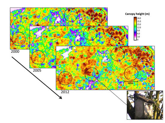
3.1. Comparison of Woodland Structure between the Different Lidar Datasets

For the 13 nest boxes occupied in either 1997 and/or 2001, the mean height in the 30 m radius plots surrounding each box increased between the 2000, 2005 and 2012 CHMs (Figure 1). Furthermore, the pair-wise differences in mean height per nest box between the 2000 and 2005 CHMs and between the 2005 and 2012 CHMs were statistically significant at p < 0.001. Across the 13 nest boxes, the overall H_mean increased from 13.01 m in 2000, to 14.57 m in 2005 and 15.47 m in 2012. The overall H_mean in the 2012 point cloud data was 14.56 m (first return only) and 11.75 m (all returns). From paired t-test results, H_mean calculated using all returns was significantly lower than when calculated using only first returns, and both were significantly lower than H_mean derived from the 2012 CHM (p < 0.001 in all cases).

Figure 1. Mean canopy height (H_mean) for the 13 occupied nest boxes as extracted from 30 m radius plots in 2000, 2005 and 2012 lidar Canopy Height Models (CHM) and from 2012 point cloud (PC) data calculated using first returns only (FR) and all returns (AR). Sample sizes: 2000 CHM 2864 raster cells; 2005 CHM 11,438 raster cells; 2012 CEH 2864 raster cells; 2012 PC FR 6298–34,499 points; 2012 PC AR 10,146–47,471 points (see Table S2).

Figure 1. Mean canopy height (H_mean) for the 13 occupied nest boxes as extracted from 30 m radius plots in 2000, 2005 and 2012 lidar Canopy Height Models (CHM) and from 2012 point cloud (PC) data calculated using first returns only (FR) and all returns (AR). Sample sizes: 2000 CHM 2864 raster cells; 2005 CHM 11,438 raster cells; 2012 CEH 2864 raster cells; 2012 PC FR 6298–34,499 points; 2012 PC AR 10,146–47,471 points (see Table S2).

3.2. Organism-Habitat Relationships Using Mean Height from 2000, 2005 and 2012 Chms

For the 2001 great tit data, the relationship between mean nestling body mass and mean height extracted from the raster CHMs had an R² value in the range 0.740–0.856 (n = 11, p < 0.001) from all three dates of lidar data and for all three methods of calculating the mean height per plot (Table 3). All of these relationships for the 2001 bird data were negative in trend. Relationships were stronger using the 2000 lidar CHM (R² range 0.810–0.856), declined slightly using the 2005 CHM (R² range 0.797–0.821) and declined further in the 2012 CHM (R² range 0.740–0.757). For all three lidar dates, the strongest relationship between mean nestling body mass in 2001 and mean height occurred when mean height was calculated only for grid cells in the CHM that were above 2 m (i.e., H_{mean > 2 m}).

In comparison to 2001, the relationships between mean nestling body mass in 1997 and mean canopy height were weaker, positive in trend and not statistically significant at p = 0.05 (although most were significant at p = 0.10). The strongest relationships with mean body mass were derived using the 2005 CHM (R² range 0.421–0.499, p < 0.10, n = 8). The 2000 CHM generated slightly weaker relationships (R² range 0.396–0.409, p < 0.10, n = 8), whilst the 2012 CHM only generated a statistically significant relationship when mean height was calculated only from grid cells above 8 m (R² = 0.433, p < 0.10, n = 8).

Table 3. Relationship between great tit nestling mean body mass in spring 1997 and 2001 and mean canopy height from raster Canopy Height Models (CHMs) generated from airborne lidar data acquired in 2000, 2005 and 2012. All relationships for 1997 have a positive trend, whereas relationships in 2001 have a negative trend. Values shown in bold are significant at p < 0.10, the underlined values are the highest R² per column.

Dataset	1997 Great Tit Data						2001 Great Tit Data
	Hmean		Hmean > 2 m		Hmean > 8 m		Hmean		Hmean > 2 m		Hmean > 8 m
	R2	p	R2	p	R2	p	R2	p	R2	p	R2	p
2000 CHM	0.409	0.088	0.405	0.090	0.396	0.094	0.838	<0.001	0.856	<0.001	0.810	<0.001
2005 CHM	0.421	0.082	0.442	0.072	0.499	0.051	0.816	<0.001	0.821	<0.001	0.797	<0.001
2012 CHM	0.319	0.145	0.356	0.118	0.433	0.076	0.740	<0.001	0.757	<0.001	0.754	<0.001

Table 3. Relationship between great tit nestling mean body mass in spring 1997 and 2001 and mean canopy height from raster Canopy Height Models (CHMs) generated from airborne lidar data acquired in 2000, 2005 and 2012. All relationships for 1997 have a positive trend, whereas relationships in 2001 have a negative trend. Values shown in bold are significant at p < 0.10, the underlined values are the highest R² per column.

Dataset	1997 Great Tit Data						2001 Great Tit Data
	Hmean		Hmean > 2 m		Hmean > 8 m		Hmean		Hmean > 2 m		Hmean > 8 m
	R2	p	R2	p	R2	p	R2	p	R2	p	R2	p
2000 CHM	0.409	0.088	0.405	0.090	0.396	0.094	0.838	<0.001	0.856	<0.001	0.810	<0.001
2005 CHM	0.421	0.082	0.442	0.072	0.499	0.051	0.816	<0.001	0.821	<0.001	0.797	<0.001
2012 CHM	0.319	0.145	0.356	0.118	0.433	0.076	0.740	<0.001	0.757	<0.001	0.754	<0.001

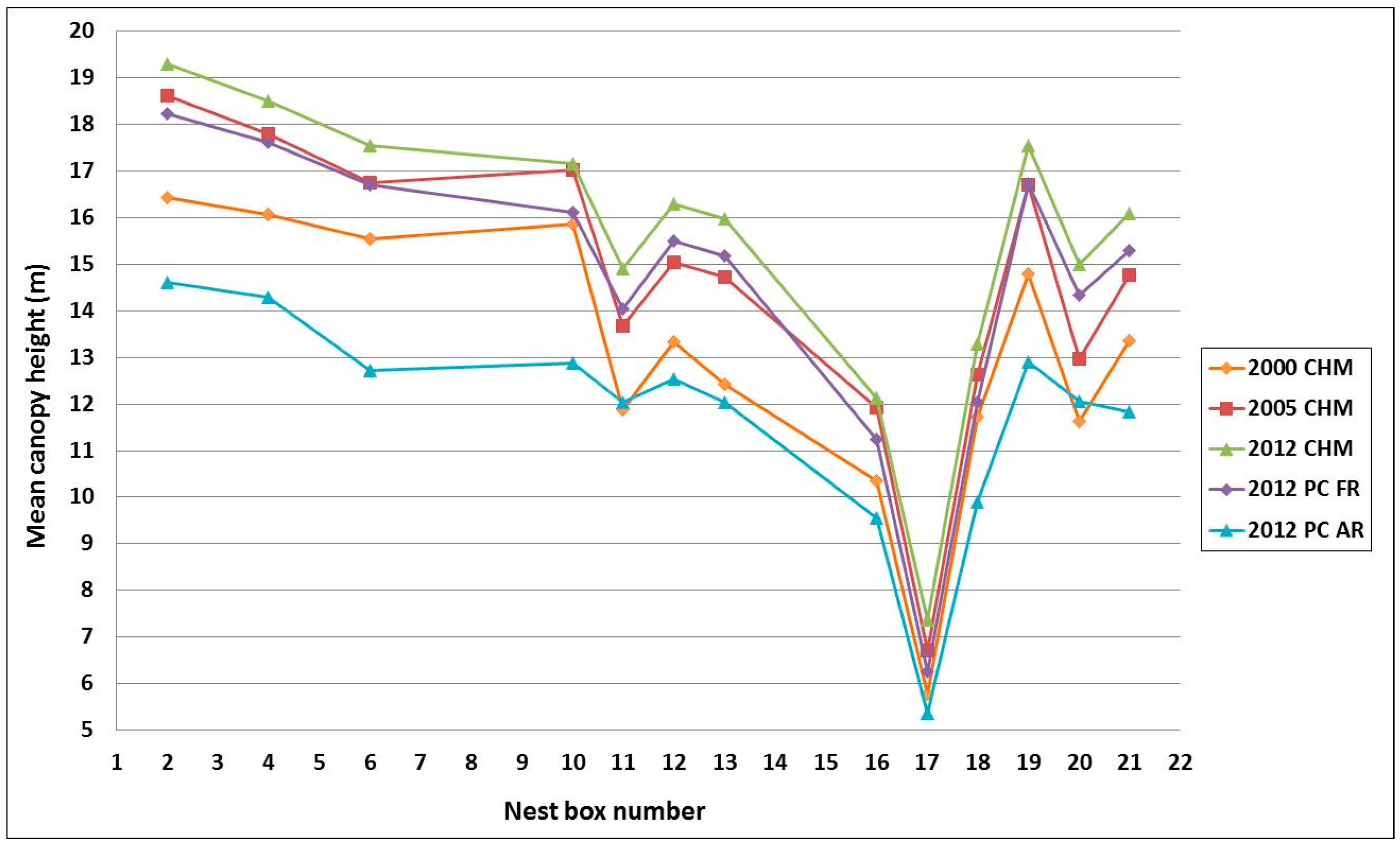
3.3. Organism–Habitat Relationships Using Mean Height from 2012 CHM and Point Cloud Data

Using the 2012 point cloud data (first return only), the relationship between mean nestling body mass and mean height had an R² value in the range 0.280–0.400 (n = 8, p = 0.177–0.093) for the 1997 breeding season and in the range 0.718–0.748 (n = 11, p < 0.001) for 2001. In all cases (i.e., both breeding seasons and mean canopy height calculated as H_mean, H_{mean > 2 m} and H_{mean > 8 m}), the relationship between mean nestling body mass and mean height around the nest box was slightly stronger when mean height was extracted from the CHM rather than from the first return point cloud (Table 4). However, the difference in R² value was never greater than 0.039. For the 1997 breeding season, there was a clear trend of H_{mean > 8 m} generating the strongest relationship for both the CHM and point cloud datasets, whilst in 2001, H_{mean > 2 m} and H_{mean > 8 m} gave almost identically strong relationships.

Table 4. Relationship between great tit nestling mean body mass in spring 1997 and 2001 and mean canopy height from a raster Canopy Height Model (CHM) and point cloud data (first return only) acquired in 2012. All relationships for 1997 have a positive trend, whereas relationships in 2001 have a negative trend. Values shown in bold are significant at p < 0.10, the underlined values are the highest R² per column.

Dataset	1997 Great Tit Data						2001 Great Tit Data
	Hmean		Hmean > 2 m		Hmean > 8 m		Hmean		Hmean > 2 m		Hmean > 8 m
	R2	p	R2	p	R2	p	R2	p	R2	p	R2	p
CHM	0.319	0.145	0.356	0.118	0.433	0.076	0.740	<0.001	0.757	<0.001	0.754	<0.001
Point cloud	0.280	0.177	0.327	0.139	0.400	0.093	0.718	<0.001	0.744	<0.001	0.748	<0.001

Table 4. Relationship between great tit nestling mean body mass in spring 1997 and 2001 and mean canopy height from a raster Canopy Height Model (CHM) and point cloud data (first return only) acquired in 2012. All relationships for 1997 have a positive trend, whereas relationships in 2001 have a negative trend. Values shown in bold are significant at p < 0.10, the underlined values are the highest R² per column.

Dataset	1997 Great Tit Data						2001 Great Tit Data
	Hmean		Hmean > 2 m		Hmean > 8 m		Hmean		Hmean > 2 m		Hmean > 8 m
	R2	p	R2	p	R2	p	R2	p	R2	p	R2	p
CHM	0.319	0.145	0.356	0.118	0.433	0.076	0.740	<0.001	0.757	<0.001	0.754	<0.001
Point cloud	0.280	0.177	0.327	0.139	0.400	0.093	0.718	<0.001	0.744	<0.001	0.748	<0.001

3.4. Organism-Habitat Relationships Using Mean Height from 2012 Point Cloud Data Systematically Reducing the Point Density

Systematically halving the number of first return points that were used to calculate the mean height (H_mean) from 2012 point cloud data (up to a total of seven times) had almost no impact on the subsequent use of those data to assess the relationship between mean height and mean nestling body mass in 2001. Thus, calculating mean height using all first return data points per plot (mean number of points 20,392; range 6298–35,499) compared with only 1/128th of all first return points per plot (mean 159 points; range 49–277), only reduced the derived relationship with mean body mass in 2001 from R² = 0.718 to R² = 0.714 (n = 11, p < 0.001). As the relationship between mean nestling body mass in 1997 and mean height per plot extracted from the 2012 lidar data was not statistically significant at p = 0.10, the effect of reducing the lidar point count on this relationship was not assessed.

3.5. Organism-Habitat Relationships Using 33 Structure Metrics from 2012 Point Cloud Data

A total of 33 structure metrics were extracted directly from the 2012 lidar point cloud for two separate datasets, (i) using all returns and (ii) using only the first returns. The relationship between each of these structure metrics and great tit mean nestling body mass in the springs of 1997 and 2001 is listed in Table 5. Taking H_mean calculated using first return data as a point of comparison with previous sections (i.e., 3.2–3.4), the relationship with this metric and mean nestling body mass in 2001 was R² = 0.718 (n = 11, p < 0.001). For the remaining 65 lidar structure metrics (generated using all and first returns), only 15 produced a stronger relationship with mean nestling body mass in 2001. Of these 15 metrics, seven were calculated using all returns and eight using only first returns; these were the height percentiles H₅₀–H₆₅ (all returns), H₂₅–H₅₀ (first returns), H_{mean > 2 m} and H_{mean > 8 m} (all and first returns), and standard deviation of height (all returns). The strongest relationship with mean nestling body mass in 2001 across all lidar point cloud metrics occurred with the standard deviation of height (H_std) calculated using all returns (R² = 0.769, p < 0.001, n = 11). A cluster of variables had relationships in the range R² = 0.744 to 0.748 (p < 0.001), including H₄₀ and H₄₅ (first returns), H₅₅ and H₆₀ (all returns), and both H_{mean > 2 m} and H_{mean > 8 m} (first returns). It is notable that these latter relationships represent only a moderate increase in the strength of relationship attained using H_mean derived from the 2012 raster CHM (R² = 0.740, n = 11, p < 0.001).

Two additional points are worth noting from Table 5 regarding the 2001 great tit breeding data. Firstly, height standard deviation (H_std) was the only metric to vary strongly when calculated using all returns and only first returns; producing a strong significant negative relationship with mean nestling body mass when calculated using all returns (R² = 0.769, p < 0.001) and a non-significant, weakly positive relationship when calculated using only the first returns (R² = 0.125, p = 0.286). Secondly, the more complex metrics than height, such as foliage height diversity, vegetation cover, canopy permeability, canopy closure and percentage returns from different vegetation layers (ground layer, understorey, overstorey) resulted in notably weaker relationships than H_mean. Only the vertical distribution ratio (VDR) gave similar strength relationships to H_mean, both using all returns (VDR: R² = 0.674, p = 0.002; H_mean: R² = 0.661, p = 0.002) and using first returns only (VDR: R² = 0.713, p < 0.001; H_mean: R² = 0.718, p < 0.001).

Table 5. Relationships between great tit nestling mean body mass in spring 1997 and 2001 and woodland structure metrics derived from 2012 lidar point cloud data. Values shown in bold are significant at p < 0.10, the underlined values are the highest R² per column.

Metric Name	1997 Great Tit Data						2001 Great Tit Data
	All Returns			First Return Only			All Returns			First Return Only
	Trend	R2	p	Trend	R2	p	Trend	R2	p	Trend	R2	p
Veg. cover	−	0.093	0.464	−	0.179	0.296	−	0.427	0.029	−	0.469	0.020
Canopy perm.	+	0.185	0.288	+	0.197	0.271	−	0.491	0.016	−	0.488	0.017
Canopy closure	+	0.222	0.234	+	0.002	0.921	−	0.440	0.026	−	0.473	0.019
H5	+	0.000	0.985	+	0.000	0.990	−	0.111	0.316	−	0.511	0.013
H10	+	0.001	0.952	+	0.025	0.708	−	0.113	0.311	−	0.643	0.003
H15	+	0.002	0.919	+	0.105	0.433	−	0.261	0.108	−	0.684	0.002
H20	+	0.016	0.760	+	0.174	0.304	−	0.386	0.041	−	0.705	0.001
H25	+	0.042	0.627	+	0.222	0.239	−	0.484	0.018	−	0.723	0.001
H30	+	0.108	0.471	+	0.264	0.192	−	0.580	0.006	−	0.731	0.001
H35	+	0.136	0.370	+	0.312	0.150	−	0.635	0.003	−	0.736	0.001
H40	+	0.166	0.317	+	0.403	0.091	−	0.679	0.002	−	0.744	0.001
H45	+	0.203	0.261	+	0.453	0.067	−	0.714	0.001	−	0.747	0.001
H50 (Hmedian)	+	0.251	0.206	+	0.469	0.061	−	0.735	0.001	−	0.726	0.001
H55	+	0.293	0.166	+	0.474	0.058	−	0.745	0.001	−	0.712	0.001
H60	+	0.397	0.094	+	0.472	0.060	−	0.746	0.001	−	0.697	0.001
H65	+	0.445	0.071	+	0.465	0.063	−	0.726	0.001	−	0.682	0.002
H70	+	0.458	0.065	+	0.457	0.066	−	0.703	0.001	−	0.675	0.002
H75	+	0.450	0.096	+	0.448	0.069	−	0.683	0.002	−	0.672	0.002
H80	+	0.439	0.073	+	0.417	0.083	−	0.674	0.002	−	0.665	0.002
H85	+	0.412	0.087	+	0.358	0.117	−	0.665	0.002	−	0.646	0.003
H90	+	0.321	0.143	+	0.270	0.187	−	0.638	0.003	−	0.620	0.004
H95	+	0.191	0.279	+	0.151	0.341	−	0.585	0.006	−	0.554	0.009
H100 (Hmax)	+	0.031	0.679	+	0.031	0.678	−	0.397	0.038	−	0.397	0.038
Hmean	+	0.284	0.174	+	0.280	0.177	−	0.661	0.002	−	0.718	0.001
Hstd	+	0.486	0.055	+	0.050	0.596	−	0.769	0.001	+	0.125	0.286
Hmean >2m	+	0.340	0.129	+	0.327	0.139	−	0.719	0.001	−	0.744	0.001
Hmean 2-8m	−	0.001	0.976	−	0.036	0.651	+	0.005	0.862	+	0.109	0.322
Hmean >8m	+	0.403	0.091	+	0.400	0.093	−	0.735	0.001	−	0.748	0.001
Pgroundlayer	−	0.153	0.338	−	0.118	0.404	+	0.416	0.032	+	0.483	0.018
Punderstorey	−	0.166	0.316	−	0.189	0.282	+	0.601	0.005	+	0.637	0.003
Poverstorey	+	0.221	0.240	+	0.136	0.368	−	0.528	0.011	−	0.577	0.007
FHD	−	0.045	0.612	−	0.082	0.491	+	0.502	0.015	+	0.589	0.006
VDR	−	0.149	0.345	−	0.344	0.126	+	0.674	0.002	+	0.713	0.001

Table 5. Relationships between great tit nestling mean body mass in spring 1997 and 2001 and woodland structure metrics derived from 2012 lidar point cloud data. Values shown in bold are significant at p < 0.10, the underlined values are the highest R² per column.

Metric Name	1997 Great Tit Data						2001 Great Tit Data
	All Returns			First Return Only			All Returns			First Return Only
	Trend	R2	p	Trend	R2	p	Trend	R2	p	Trend	R2	p
Veg. cover	−	0.093	0.464	−	0.179	0.296	−	0.427	0.029	−	0.469	0.020
Canopy perm.	+	0.185	0.288	+	0.197	0.271	−	0.491	0.016	−	0.488	0.017
Canopy closure	+	0.222	0.234	+	0.002	0.921	−	0.440	0.026	−	0.473	0.019
H5	+	0.000	0.985	+	0.000	0.990	−	0.111	0.316	−	0.511	0.013
H10	+	0.001	0.952	+	0.025	0.708	−	0.113	0.311	−	0.643	0.003
H15	+	0.002	0.919	+	0.105	0.433	−	0.261	0.108	−	0.684	0.002
H20	+	0.016	0.760	+	0.174	0.304	−	0.386	0.041	−	0.705	0.001
H25	+	0.042	0.627	+	0.222	0.239	−	0.484	0.018	−	0.723	0.001
H30	+	0.108	0.471	+	0.264	0.192	−	0.580	0.006	−	0.731	0.001
H35	+	0.136	0.370	+	0.312	0.150	−	0.635	0.003	−	0.736	0.001
H40	+	0.166	0.317	+	0.403	0.091	−	0.679	0.002	−	0.744	0.001
H45	+	0.203	0.261	+	0.453	0.067	−	0.714	0.001	−	0.747	0.001
H50 (Hmedian)	+	0.251	0.206	+	0.469	0.061	−	0.735	0.001	−	0.726	0.001
H55	+	0.293	0.166	+	0.474	0.058	−	0.745	0.001	−	0.712	0.001
H60	+	0.397	0.094	+	0.472	0.060	−	0.746	0.001	−	0.697	0.001
H65	+	0.445	0.071	+	0.465	0.063	−	0.726	0.001	−	0.682	0.002
H70	+	0.458	0.065	+	0.457	0.066	−	0.703	0.001	−	0.675	0.002
H75	+	0.450	0.096	+	0.448	0.069	−	0.683	0.002	−	0.672	0.002
H80	+	0.439	0.073	+	0.417	0.083	−	0.674	0.002	−	0.665	0.002
H85	+	0.412	0.087	+	0.358	0.117	−	0.665	0.002	−	0.646	0.003
H90	+	0.321	0.143	+	0.270	0.187	−	0.638	0.003	−	0.620	0.004
H95	+	0.191	0.279	+	0.151	0.341	−	0.585	0.006	−	0.554	0.009
H100 (Hmax)	+	0.031	0.679	+	0.031	0.678	−	0.397	0.038	−	0.397	0.038
Hmean	+	0.284	0.174	+	0.280	0.177	−	0.661	0.002	−	0.718	0.001
Hstd	+	0.486	0.055	+	0.050	0.596	−	0.769	0.001	+	0.125	0.286
Hmean >2m	+	0.340	0.129	+	0.327	0.139	−	0.719	0.001	−	0.744	0.001
Hmean 2-8m	−	0.001	0.976	−	0.036	0.651	+	0.005	0.862	+	0.109	0.322
Hmean >8m	+	0.403	0.091	+	0.400	0.093	−	0.735	0.001	−	0.748	0.001
Pgroundlayer	−	0.153	0.338	−	0.118	0.404	+	0.416	0.032	+	0.483	0.018
Punderstorey	−	0.166	0.316	−	0.189	0.282	+	0.601	0.005	+	0.637	0.003
Poverstorey	+	0.221	0.240	+	0.136	0.368	−	0.528	0.011	−	0.577	0.007
FHD	−	0.045	0.612	−	0.082	0.491	+	0.502	0.015	+	0.589	0.006
VDR	−	0.149	0.345	−	0.344	0.126	+	0.674	0.002	+	0.713	0.001

It should be noted that by performing 33 regression calculations from a single dataset, there is a ca. 82% chance of identifying a false positive (i.e., type I error) in these results. Taking a p value of 0.10 as representing statistical significance for a single test, the Bonferroni correction gives p = 0.003 for the entire dataset. Given this significance level, for the 2001 great tit data only the following first return point cloud variables gave a statistically significant result when regressed with mean nestling body mass: H₁₀–H₈₅, H_mean, H_{mean > 2 m}, H_{mean > 8 m}, P_understorey, and VDR. Using all returns in the 2012 lidar point cloud, only the following variables gave statistically significant regression results: H₃₅–H₉₀, H_mean, H_std, H_{mean > 2 m}, H_{mean > 8 m}, and VDR. However, it should also be noted that the use of Bonferroni correction in ecology has been questioned [43,44].

For the 1997 great tit data, all of the relationships with the lidar variables were weaker than for the 2001 data and, with the exception of vegetation cover (all and first returns) and height standard deviation (first returns only), had the opposite trend. None of these latter mentioned relationships were statistically significant at p = 0.10 (Table 5). As with the 2001 bird data, the lidar variables that generated stronger relationships with nestling body mass than H_mean in 1997 were height percentiles, although in this case H₅₅–H₉₀ (all returns) and H₃₅–H₈₅ (first returns), H_{mean > 2 m} and H_{mean > 8 m} (all and first returns), H_std (all returns), and in addition VDR (first returns only). However, of these it should be noted that only H₆₀–H₈₅ (all returns), H₄₀–H₈₀ (first returns), H_{mean >8m} (all and first returns) and H_std (all returns) were statistically significant relationships at p = 0.10. (None of these were significant using the Bonferroni correction of p = 0.003). As with the 2001 great tit data, the strongest overall relationship (R² = 0.486, p = 0.055, n = 8) occurred with standard deviation of height using all returns. The next strongest relationship (R² = 0.474, p = 0.058, n = 8) occurred with the percentile H₅₅ from first return lidar points. Looking specifically at the canopy height percentiles, for the 1997 and 2001 great tit relationships the strongest using all returns occurred for H₇₀ in 1997 and H₆₀ in 2001, and using only first returns occurred for H₅₅ in 1997 and H₄₅ in 2001.

4. Discussion

4.1. Great Tit Breeding Habitat Requirements

The results of this study show an inversion in the trend of relationships between lidar-derived woodland structure metrics and mean nestling body mass in 1997 compared with 2001. As published previously [29], this may be explained by differences in weather conditions which influence the type of woodland structure that provides the best foraging conditions for parent birds during the rearing of nestlings. Nonetheless, although optimum structure may differ from year to year depending on the weather, the lidar-derived metrics that best characterise this structure have been shown to be consistent. Thus, looking at the point cloud metrics derived from the 2012 lidar data, key woodland structure metrics that can be identified as important in both years were mean overstorey canopy height (i.e., H_{mean > 8 m}) and canopy height percentiles (calculated using all returns and only first returns) and height standard deviation (calculated using all returns).

In general, stronger relationships were attained with mean nestling body mass when using median height per plot (H_median) rather than mean height (H_mean). Furthermore, the relationships were stronger still when using height percentiles immediately adjacent to the median with first returns (i.e., H₄₅ and H₅₅ for 2001 and 1997 bird data, respectively), or using height percentiles above the median with all returns (i.e., H₆₀ and H₇₀ for 2001 and 1997, respectively). The histogram of all returns is skewed towards lower values compared with the histogram of first returns, since the first returns characterise the canopy top whilst all returns include data points from within the canopy or sub-canopy. Thus, for the 11 sample plots surrounding occupied nest boxes in 2001, H₄₅ (first returns) and H₆₀ (all returns) both describe a canopy height of ca. 14.5 m, whereas for the eight sample plots in 1997, H₅₅ (first returns) and H₇₀ (all returns) both describe canopy height of ca. 16.5 m. In both years, there would therefore appear to be an optimum vegetation height for foraging, and the use of height percentiles (whether from all returns or only first returns) allows this optimum height to be identified.

H_{mean > 2 m} and H_{mean > 8 m} generally resulted in stronger relationships with mean nestling body mass than H_mean for both 1997 and 2001. Thus, removing the ground vegetation and/or understorey layers in calculating mean height per sample area around the nest box typically strengthened relationships with mean nestling body mass. In 2001, the relationship between mean nestling body mass and the percentage of returns in the overstorey (P_overstorey) was weaker than that with mean height (H_mean), for both all and first return data (with a similar pattern in the non-significant relationships in 1997). As the proportional coverage of overstorey in the 30 m radius sample areas varied across the range 40%–97% for the occupied nest boxes in both 1997 and 2001, this suggests that it was not so much the amount of overstorey but its height that was an important factor in determining foraging habitat quality in each year. The strongest relationships with mean nestling body mass in both years occurred with standard deviation of height from all returns, but no relationships at all occurred with standard deviation of height from only first returns. This showed that variation in height at the top of the vegetation canopy was not important in determining foraging habitat quality, whilst variation throughout the woodland vertical profile evidently was. Note that the above relationships were moderate and positive in 1997, but strong and negative in 2001. In addition, moderate to strong positive relationships occurred in 2001 between mean nestling body mass and both foliage height diversity and the vertical distribution ratio, highlighting the importance of a sub-canopy or understorey. Piecing these results together it would seem that in 2001, when foraging was difficult due to poor weather, the best foraging conditions occurred (within limits not fully identified in this study) where there was less overstorey coverage, a greater presence of shrub layer and/or understorey, where overstorey canopy height was lower (optimum at around 14.5 m), and where there was less variation in canopy vertical profile (suggesting the need for a more continuous understorey layer). By contrast, in 1997 when foraging conditions were good due to more benign weather, the optimum woodland structure for foraging involved a taller canopy (optimum 16.5 m) with greater variation in canopy vertical profile (implying a lesser need for continuous understorey). It is thus likely that during poor weather, the main prey of the great tits (tree-dwelling caterpillars) is more abundant at lower heights due to wash-out from the higher canopy, with the understorey providing more sheltered foraging for parent birds.

Although the foraging niche of the great tit in British woodland is one of the best described in avian ecology [45,46,47], the lidar data have identified detailed elements of woodland structure that determine the quality of foraging habitat under different weather conditions during the breeding season. Great tits may be particularly vulnerable to poor weather because the larger sizes of caterpillars that are optimal for the growth of their nestlings [48] are likely to be less abundant under such conditions (i.e., slower larval growth rates combined with greater losses to smaller competitor species, such as blue tits, that prefer smaller caterpillars [49]). Furthermore, with climate change likely to increase the incidence of extreme weather and its impact on woodland birds [50,51], knowledge of woodland structures most favourable for foraging under a range of different conditions is vital.

4.2. Assessment of Results against Study Aims

The woodland showed a significant increase in height in the sample areas around occupied nest boxes between 2000, 2005 and 2012 as might be expected from tree growth. However, the rate of increase in mean canopy height was not even per nest box (mean height would be affected by loss of woody material as well as growth), and therefore the rank position of the nest boxes by mean height changed between the three years of lidar data acquisition. This combined to affect the results of the regression analyses between mean height and mean nestling body mass. For the 2001 breeding data, results showed a decline in the strength of relationships between mean height and mean nestling body mass across the three lidar datasets. This would be expected, as the 2000, 2005 and 2012 lidar data had a one year, four year and 11 year time-lag, respectively, to the bird breeding data. However, the decline in the strength of the relationship amounted to less than 1% of total variance explained for every year of time difference between breeding data and lidar data. For the 1997 bird breeding data, the strongest relationships between mean height and mean nestling body mass occurred using the 2005 lidar data, implying that contemporaneous field and lidar data are not always a necessity to achieve maximum strength relationships. However, this seems likely to be an effect of ‘noise’ in this weaker relationship. Nonetheless, the fact that it remained detectable across a time-lag of at least eight years is broadly similar to the findings for the 2001 breeding data.

The process of rasterising the 2012 lidar data to derive a CHM significantly affected the mean height statistics for each sample plot compared with values extracted directly from the point cloud. This had an impact on the derived relationships between mean height and mean nestling body mass. For both the 1997 and 2001 breeding data, stronger relationships between mean height and mean nestling body mass were generated using the CHM data than the point cloud data (first return only). Interestingly, this was the case despite the mean canopy heights from the CHM being significantly greater than those extracted from the point cloud. The CHM had greater mean height values because the rasterisation process took the maximum height per 1 m grid cell. Selecting mean height per grid cell would have lowered the height value in most cells and therefore also the overall mean height value calculated per 30 m sample plot around each nest box. Rasterising a point cloud using either a mean or maximum value per cell would likely have an uneven impact on differently structured forest, and hence subsequent use of those data in organism-habitat modelling. Other methods of rasterising lidar data into a CHM (such as those employed with the 2000 and 2005 datasets) would likely have generated other differences in derived mean height. It should be noted that it was a deliberate decision, rather than an oversight, not to re-process the older lidar datasets using the more up-to-date methods employed with the 2012 data acquisition. The reason for this was that many older lidar datasets held in archives may only be available as processed raster models generated shortly after data acquisition. The aim here was to assess the potential usefulness of such datasets in organism–habitat modelling if they are all that is available.

Reducing the number of lidar returns that were included in the calculation of mean height per 30 m radius plot had very little effect on the resulting mean height value, and therefore no significant impact on the subsequent use of those data to assess the relationship between mean height and mean nestling body mass using the 2001 breeding data.

The comparison of 33 different lidar metrics in regression analyses of woodland structure and mean nestling body mass showed mean height to be one of the better performing variables. However, the required structural profile was summarised better by other single descriptive measures, such as median height or specific height percentiles. Furthermore, greater explanatory power was derived by considering several descriptive measures which supply complementary information about the canopy profile, such as standard deviation of all lidar returns and mean overstorey height. Thus, our understanding of how the full structural variation of woodland influences habitat quality for great tits in different breeding seasons (and under different weather conditions) has expanded from that presented in [29] through a consideration of the wider set of variables extracted from the 2012 lidar point cloud data. Of particular importance was the additional information available from multiple return data and the separate analysis of all return and first return only data.

Studies at a range of field sites for other bird species (and other taxa) have shown a host of different lidar metrics to provide the most relevant characterisation of woodland structure to explain presence, abundance, or biological activity. For example, for the black-throated blue warbler (Dendroica caerulescens) in the northern hardwood forests of Hubbard Brook, New Hampshire, canopy height, elevation and canopy complexity were found to be key characteristics of frequently occupied habitat [32]. Horizontal structure (i.e., relative tree canopy cover) was demonstrated to be a key habitat variable determining the presence of capercaillie (Tetrao urogallus) in a forest reserve in the Swiss Pre-Alps [8]. For the black-capped vireo (Vireo atricapilla) in the Fort Hood Military Reservation, Texas, mean height, canopy cover, and edge density were useful predictive variables, although not as important as vegetation and soil type [52]. Measures of forest vertical structure (e.g., mean and standard deviation of canopy height) and horizontal patterns of vertical structure (assessed by both semivariograms and lacunarity analysis), together with elevation, land-cover and hydrography data were found useful in predictive distribution modelling for the red-cockaded woodpecker (Picoides borealis, Vieillot) in a forested catchment in North Carolina [31]. For the red-naped sapsucker (Sphyrapicus nuchalis) in northern Idaho, key airborne lidar variables for predicting breeding site selection were foliage height diversity, the distance between major strata in the canopy vertical profile, and vegetation density close to the ground [17]. Moving away from birds as the focal species, in a study of the Pacific fisher in the Sierra Nevada Mountains, California, tree height and slope were shown to be important variables within a 20 m radius of a denning tree, but forest structure and complexity became more important between 20 m and 50 m [19]. These studies show that an understanding of the ecology of both the focal species and the study ecosystem is required when identifying the most appropriate use of airborne lidar data in investigating organism-habitat relationships. With one exception [33], no other study has assessed the impacts of time-series lidar data on their use in ecological assessment.

4.3. Applicability of Results to Other Ecological Systems

This case study has examined the breeding data for a single species (great tit) at a single site (Monks Wood), in just two breeding seasons (spring 1997 and 2001). Furthermore, the sample sizes were small, with mean nestling body mass calculated over just eight nest boxes in 1997 and eleven boxes in 2001. This particularly influenced the statistical significance levels of the relationships derived using the 1997 bird breeding data, increasing the uncertainty of the findings. These are obvious limitations, and therefore the findings may not be applicable across all ecological studies seeking structure-based organism-habitat relationships. In this particular case study, measures of canopy closure were not particularly relevant to the relationships under investigation. This helped make the mean height a robust summarising measure that consistently provided statistically significant relationships with mean nestling body mass in 2001 despite variations in the lidar data characteristics assessed (i.e., time-lag with field data, spatial sampling density, raster or point cloud data processing). The lack of impact of the time-lag between lidar and field data was also influenced by the relatively mature state of Monks Wood and minimal active management (and natural change such as tree fall) within the sample area surrounding each nest box. Thus, because of the feeding niche of the great tit and the ecological state of the field site in this study, mean height extracted from airborne lidar data was shown to be a robust measure, providing a good overall summary of woodland structure required for parental foraging during the breeding season. Also, although the specific ecological relationships reported here for the great tit may not apply to other woodland species with different foraging niches (e.g., the marsh tit Poecile palustris which has a greater association with woodland understorey, [53]), it seems likely that relationships for other species in mature woodland may be similarly robust with respect to lidar data characteristics.

5. Conclusions

In spring 2001, the relationship between woodland structure (assessed as mean height) and nest success for great tits was robust to the extent that it could be detected strongly and with a high level of statistical significance from lidar data, with relatively little impact of lidar data characteristics. For example, the relationship between mean height (H_mean) and mean nestling body mass had an R² value of 0.856, 0.821 and 0.757 (p < 0.001 in all cases) using a lidar-derived raster Canopy Height Model (CHM) acquired in the years 2000, 2005 and 2012, respectively. This relationship dropped to R² = 0.718 (p < 0.001) when H_mean was calculated directly from 2012 point cloud data (using first returns only), and fell only slightly further to R² = 0.714 (p < 0.001) when the point density was reduced to just 1/128th of the original point count. Furthermore, when a range of metrics were derived from the 2012 lidar point cloud data (33 metrics each calculated using all returns and only first returns), only 15 metrics gave a stronger relationship with mean nestling body mass than H_mean (seven metrics using all returns, and eight metrics using only first returns). Of these, the strongest relationship with mean nestling body mass occurred using the standard deviation of height (H_std) calculated using all returns (R² = 0.769, p < 0.001, n = 11). Thus, for a breeding season in which harsh weather conditions made successful breeding difficult, it made only a moderate difference to the strength with which the relationship between canopy height and breeding success could be estimated as to whether the lidar data were acquired within one year or 11 years of the field data on bird breeding, whether woodland height was derived directly from lidar point clouds or from raster canopy height models, and whether thousands, hundreds or just tens of lidar data points were used in the calculation of mean height per plot. For the 1997 great tit breeding season, a somewhat benign year in terms of weather conditions, no statistically significant relationship (at p = 0.05) with mean nestling body mass was attained with any of the lidar datasets or variables. The strongest relationship occurred with mean height extracted from the 2005 raster CHM using only those grid cells with a value above 8 m (i.e., H_{mean > 8 m}); R² = 0.499, p = 0.051, n = 8. For this breeding season, forest structure (however, assessed using lidar data) was shown to have a more moderate influence on bird breeding success.

The results of this study thus show that for relatively mature and undisturbed woodland, ecologists should not feel prohibited in using lidar data to explore organism–habitat relationships because of perceived data quality issues, such as a time-lag, low sampling density, or unavailability of point cloud data and the associated ability to derive more complex structure metrics. Uniquely, we have shown that if a relationship between biological activity and woodland canopy structure is robust (as in the 2001 great tit data), then the use of lower quality lidar data (as specified above) is unlikely to prevent such relationships from being discovered in a stable-state ecosystem. A time-lag between lidar data acquisition and field data would, of course, be expected to have a much greater impact in a more dynamic system, such as early successional or coppiced woodland. Less robust relationships (as in the 1997 great tit data) may be harder to detect across longer time lags, and in relation to other lidar quality issues, so this would have to be borne in mind when interpreting results.

References

1. MacArthur, R.H.; MacArthur, J. On bird species diversity. Ecology 1961, 42, 594–598. [Google Scholar] [CrossRef]
2. Turner, W.; Spector, S.; Gardiner, N.; Fladeland, M.; Sterling, E.; Steininger, M. Remote sensing for biodiversity science and conservation. Trends Ecol. Evol. 2003, 18, 306–314. [Google Scholar] [CrossRef]
3. Bergen, K.M.; Goetz, S.J.; Dubayah, R.O.; Henebry, G.M.; Hunsaker, C.T.; Imhoff, M.L.; Nelson, R.F.; Parker, G.G.; Radeloff, V.C. Remote sensing of vegetation 3-D structure for biodiversity and habitat: Review and implications for lidar and radar spaceborne missions. J. Geophys. Res.: Biogeosci. 2009, 114. [Google Scholar] [CrossRef]
4. Nelson, R.; Keller, C.; Ratnaswamy, M. Locating and estimating the extent of Delmarva fox squirrel habitat using an airborne LiDAR profiler. Remote Sens. Environ. 2005, 96, 292–301. [Google Scholar] [CrossRef]
5. Coops, N.C.; Duffe, J.; Koot, C. Assessing the utility of lidar remote sensing technology to identify mule deer winter habitat. Can. J. Remote Sens. 2010, 36, 81–88. [Google Scholar] [CrossRef]
6. Garabedian, J.E.; McGaughey, R.J.; Reutebuch, S.E.; Parresol, B.R.; Kilgo, J.C.; Moorman, C.E.; Peterson, M.N. Quantitative analysis of woodpecker habitat using high-resolution airborne LiDAR estimates of forest structure and composition. Remote Sens. Environ. 2014, 145, 68–80. [Google Scholar] [CrossRef]
7. Vogeler, J.C.; Hudak, A.T.; Vierling, L.A.; Vierling, K.T. Lidar-derived canopy architecture predicts brown creeper occupancy of two western coniferous forests. Condor 2013, 115, 614–622. [Google Scholar] [CrossRef]
8. Graf, R.F.; Mathys, L.; Bollmann, K. Habitat assessment for forest dwelling species using LiDAR remote sensing: Capercaillie in the Alps. For. Ecol. Manag. 2009, 257, 160–167. [Google Scholar] [CrossRef]
9. Hinsley, S.A.; Hill, R.A.; Fuller, R.J.; Bellamy, P.E.; Rothery, P. Bird species distributions across woodland canopy structure gradients. Community Ecol. 2009, 10, 99–110. [Google Scholar] [CrossRef]
10. Eldegard, K.; Dirksen, J.W.; Orka, H.O.; Halvorsen, R.; Naesset, E.; Gobakken, T.; Ohlson, M. Modelling bird richness and bird species presence in a boreal forest reserve using airborne laser-scanning and aerial images. Bird Study 2014, 61, 204–219. [Google Scholar] [CrossRef]
11. Farrell, S.L.; Collier, B.A.; Skow, K.L.; Long, A.M.; Campomizzi, A.J.; Morrison, M.L.; Hays, K.B.; Wilkins, R.N. Using LiDAR-derived vegetation metrics for high-resolution, species distribution models for conservation planning. Ecosphere 2013, 4. [Google Scholar] [CrossRef]
12. Zellweger, F.; Braunisch, V.; Baltensweiller, A.; Bollmann, K. Remotely sensed forest structural complexity predicts multi species occurrence at the landscape scale. For. Ecol. Manag. 2013, 307, 303–312. [Google Scholar] [CrossRef]
13. Vierling, K.T.; Vierling, L.A.; Gould, W.A.; Martinuzzi, S.; Clawges, R.M. Lidar: Shedding new light on habitat characterization and modelling. Front. Ecol. Environ. 2008, 6, 90–98. [Google Scholar] [CrossRef]
14. Bellamy, P.E.; Hill, R.A.; Rothery, P.; Hinsley, S.A.; Fuller, R.J.; Broughton, R.K. Willow warbler Phylloscopus trochilus habitat in woods with different structure and management in southern England. Bird Study 2009, 56, 338–348. [Google Scholar] [CrossRef]
15. Clawges, R.; Vierling, K.; Vierling, L.; Rowell, E. The use of airborne lidar to assess avian species diversity, density, and occurrence in a pine/aspen forest. Remote Sens. Environ. 2008, 112, 2064–2073. [Google Scholar] [CrossRef]
16. Swatantran, A.; Dubayah, R.; Goetz, S.; Hofton, M.; Betts, M.G.; Sun, M.; Simard, M.; Holmes, R. Mapping migratory bird prevalence using remote sensing data fusion. PLoS One 2012, 7. [Google Scholar] [CrossRef] [PubMed]
17. Vierling, L.A.; Vierling, K.T.; Adam, P.; Hudak, A.T. Using satellite and airborne lidar to model woodpecker habitat occupancy at the landscape scale. PLoS One 2013, 8. [Google Scholar] [CrossRef] [PubMed]
18. Palminteri, S.; Powell, G.V.N.; Asner, G.P.; Peres, C.C. LiDAR measurements of canopy structure predict spatial distribution of a tropical mature forest primate. Remote Sens. Environ. 2012, 127, 98–105. [Google Scholar] [CrossRef]
19. Zhao, F.; Sweitzer, R.A.; Guo, Q.; Kelly, M. Characterizing habitats associated with fisher den structures in the Southern Sierra Nevada, California using discrete return lidar. For. Ecol. Manag. 2012, 280, 112–119. [Google Scholar] [CrossRef]
20. Melin, M.; Packalen, P.; Matala, J.; Mehtalalo, L.; Pusenius, J. Assessing and modeling moose (Alces alces) habitats with airborne laser scanning data. Int. J. Appl. Earth Obs. 2013, 23, 389–396. [Google Scholar] [CrossRef]
21. Flaherty, S.; Lurz, P.W.W.; Patenaude, G. Use of LiDAR in the conservation management of the endangered red squirrel (Sciurus vulgaris L.). J. Appl. Remote Sens. 2014, 8. [Google Scholar] [CrossRef]
22. Jung, K.; Kaiser, S.; Bohm, S.; Nieschulze, J.; Kalko, E.K.V. Moving in three dimensions: Effects of structural complexity on occurrence and activity of insectivorous bats in managed forest stands. J. Appl. Ecol. 2012, 49, 523–531. [Google Scholar] [CrossRef]
23. Müller, J.; Mehr, M.; Bässler, C.; Fenton, M.B.; Hothorn, T.; Pretzsch, H.; Klemmt, H.J.; Brandl, R. Aggregative response in bats: Prey abundance versus habitat. Oecologia 2012, 169, 673–684. [Google Scholar] [CrossRef] [PubMed]
24. Lone, K.; Loe, L.E.; Gobakken, T.; Linnell, J.D.C.; Odden, J.; Remmen, J.; Mysterud, A. Living and dying in a multi-predator landscape of fear: Roe deer are squeezed by contrasting pattern of predation risk imposed by lynx and humans. Oikos 2014, 123, 641–651. [Google Scholar] [CrossRef]
25. Ewald, M.; Dupke, C.; Heurich, M.; Muller, J.; Reineking, B. LiDAR remote sensing of forest structure and GPS telemetry data provide insights on winter habitat selection of European roe deer. Forests 2014, 5, 1374–1390. [Google Scholar] [CrossRef]
26. Melin, M.; Matala, J.; Mehtatalo, L.; Tiilikainen, R.; Tikkanen, O.P.; Maltamo, M.; Pusenius, J.; Packalen, P. Moose (Alces alces) reacts to high summer temperatures by utilizing thermal shelters in boreal forests—An analysis based on airborne laser scanning of the canopy structure at moose locations. Glob. Change Biol. 2014, 20, 1115–1125. [Google Scholar] [CrossRef]
27. Hinsley, S.A.; Hill, R.A.; Gaveau, D.L.A.; Bellamy, P.E. Quantifying woodland structure and habitat quality for birds using airborne laser scanning. Funct. Ecol. 2002, 16, 851–857. [Google Scholar] [CrossRef]
28. Hill, R.A.; Hinsley, S.A.; Gaveau, D.L.A.; Bellamy, P.E. Predicting habitat quality for Great Tits (Parus major) with airborne laser scanning data. Int. J. Remote Sens. 2004, 25, 4851–4855. [Google Scholar] [CrossRef]
29. Hinsley, S.A.; Hill, R.A.; Bellamy, P.E.; Balzter, H. The application of lidar in woodland bird ecology: Climate, canopy structure, and habitat quality. Photogramm. Eng. Rem. Sens. 2006, 72, 1399–1406. [Google Scholar] [CrossRef]
30. Seavy, N.E.; Viers, J.H.; Wood, J.K. Riparian bird response to vegetation structure: A multiscale analysis using LiDAR measurements of canopy height. Ecol. Appl. 2009, 19, 1848–1857. [Google Scholar] [CrossRef] [PubMed]
31. Smart, L.S.; Swenson, J.J.; Christensen, N.L.; Sexton, J.O. Three-dimensional characterization of pine forest type and red-cockaded woodpecker habitat by small-footprint, discrete-return lidar. For. Ecol. Manag. 2012, 281, 100–110. [Google Scholar] [CrossRef]
32. Goetz, S.J.; Steinberg, D.; Betts, M.G.; Holmes, R.T.; Doran, P.J.; Dubayah, R.; Hofton, M. Lidar remote sensing variables predict breeding habitat of a neotropical migrant bird. Ecology 2010, 91, 1569–1576. [Google Scholar] [CrossRef] [PubMed]
33. Vierling, K.T.; Swift, C.E.; Hudak, A.T.; Vogeler, J.C.; Vierling, L.A. Does the time lag between wildlife field data collection and LiDAR data acquisition matter for studies of wildlife distributions? A case study using bird communities. Remote Sens. Lett. 2014, 5, 185–193. [Google Scholar] [CrossRef]
34. Patenaude, G.; Hill, R.A.; Milne, R.; Gaveau, D.L.A.; Briggs, B.B.J.; Dawson, T.P. Quantifying forest above ground carbon content using LiDAR remote sensing. Remote Sens. Environ. 2004, 93, 368–380. [Google Scholar] [CrossRef]
35. Hill, R.A.; Thomson, A.G. Mapping woodland species composition and structure using airborne spectral and LiDAR data. Int. J. Rem. Sens. 2005, 26, 3763–3779. [Google Scholar] [CrossRef]
36. Massey, M.E.; Welch, R.C. Monks Wood National Nature Reserve: The Experience of 40 Years 1953–1993; English Nature: Peterborough, UK, 1993. [Google Scholar]
37. Hill, R.A.; Wilson, A.K.; George, M.; Hinsley, S.A. Mapping tree species in temperate deciduous woodland using time-series multi-spectral data. Appl. Veg. Sci. 2010, 13, 86–99. [Google Scholar] [CrossRef]
38. Hill, R.A.; Broughton, R.K. Mapping the understorey of deciduous woodland from leaf-on and leaf-off airborne LiDAR data: A case study in lowland Britain. ISPRS J. Photogramm. 2009, 64, 223–233. [Google Scholar] [CrossRef]
39. Hinsley, S.A.; Rothery, P.; Bellamy, P.E. Influence of woodland area on breeding success in Great Tits (Parus major) and Blue Tits (Parus caeruleus). J. Avian Biol. 1999, 3, 271–281. [Google Scholar] [CrossRef]
40. Przybylo, R.; Wiggins, D.A.; Merila, J. Breeding success in Blue Tits: Good territories or good parents? J. Avian Biol. 2001, 32, 214–218. [Google Scholar] [CrossRef]
41. Gaveau, D.L.A.; Hill, R.A. Quantifying canopy height underestimation by laser pulse penetration in small-footprint airborne laser scanning data. Can. J. Remote Sens. 2003, 29, 650–657. [Google Scholar] [CrossRef]
42. Zhang, K.Q.; Chen, S.C.; Whitman, D.; Shyu, M.L.; Yan, J.H.; Zhang, C.C. A progressive morphological filter for removing non-ground measurements from airborne lidar data. IEEE Trans. Geosci. Remote Sens. 2003, 41, 872–882. [Google Scholar] [CrossRef]
43. Moran, M.D. Arguments for rejecting the sequential Bonferroni in ecological studies. Oikos 2003, 100, 403–405. [Google Scholar] [CrossRef]
44. Nakagawa, S. A farewell to Bonferroni: The problems of low statistical power and publication bias. Behav. Ecol. 2004, 15, 1044–1045. [Google Scholar] [CrossRef]
45. Lack, D. Ecological Isolation in Birds; Blackwell Scientific Publications: Oxford, UK, 1971. [Google Scholar]
46. Perrins, C.M. British Tits; Collins: London, UK, 1979. [Google Scholar]
47. Gosler, A. The Great Tit; Hamlyn Limited: London, UK, 1993. [Google Scholar]
48. Naef-Daenzer, B.; Keller, L.F. The foraging performance of great and blue tits (Parus major and P. caeruleus) in relation to caterpillar development and its consequences for nestling growth and fledging weight. J. Anim. Ecol. 1999, 57, 607–697. [Google Scholar]
49. Minot, E.O. Effects of interspecific competition for food in breeding blue and great tits. J. Anim. Ecol. 1981, 50, 375–385. [Google Scholar] [CrossRef]
50. Matthysen, E.; Adriaensen, F.; Dhondt, A.A. Multiple responses to increasing spring temperatures in the breeding cycle of blue and great tits (Cyanistes caeruleus, Parus. major). Glob. Change Biol. 2011, 17, 1–16. [Google Scholar] [CrossRef]
51. Whitehouse, M.J.; Harrison, N.M.; Mackenzie, J.A.; Hinsley, S.A. Preferred habitat of breeding birds may be compromised by climate change: unexpected effects of an exceptionally cold, wet spring. PLoS One 2013, 8. [Google Scholar] [CrossRef] [PubMed]
52. Wilsey, C.B.; Lawler, J.J.; Cimprich, D.A. Performance of habitat suitability models for the endangered black-capped vireo built with remotely-sensed data. Remote Sens. Environ. 2012, 119, 35–42. [Google Scholar] [CrossRef]
53. Broughton, R.K.; Hill, R.A.; Freeman, S.N.; Hinsley, S.A. Describing habitat occupation by wood land birds with territory mapping and remotely sensed data: An example using the Marsh Tit (Poecile palustris). Condor 2012, 114, 812–822. [Google Scholar] [CrossRef] [Green Version]