
The Effects of Point or Polygon Based Training Data on RandomForest Classification Accuracy of Wetlands

Abstract
:
1. Introduction
2. Methods
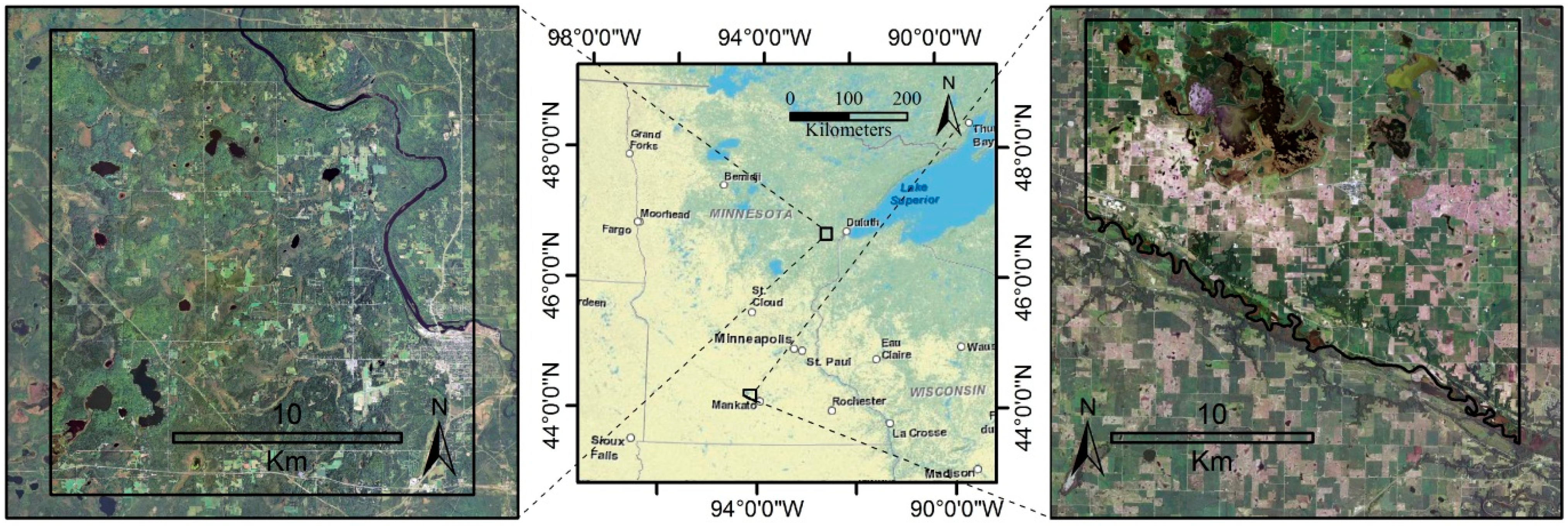
2.1. Study Areas
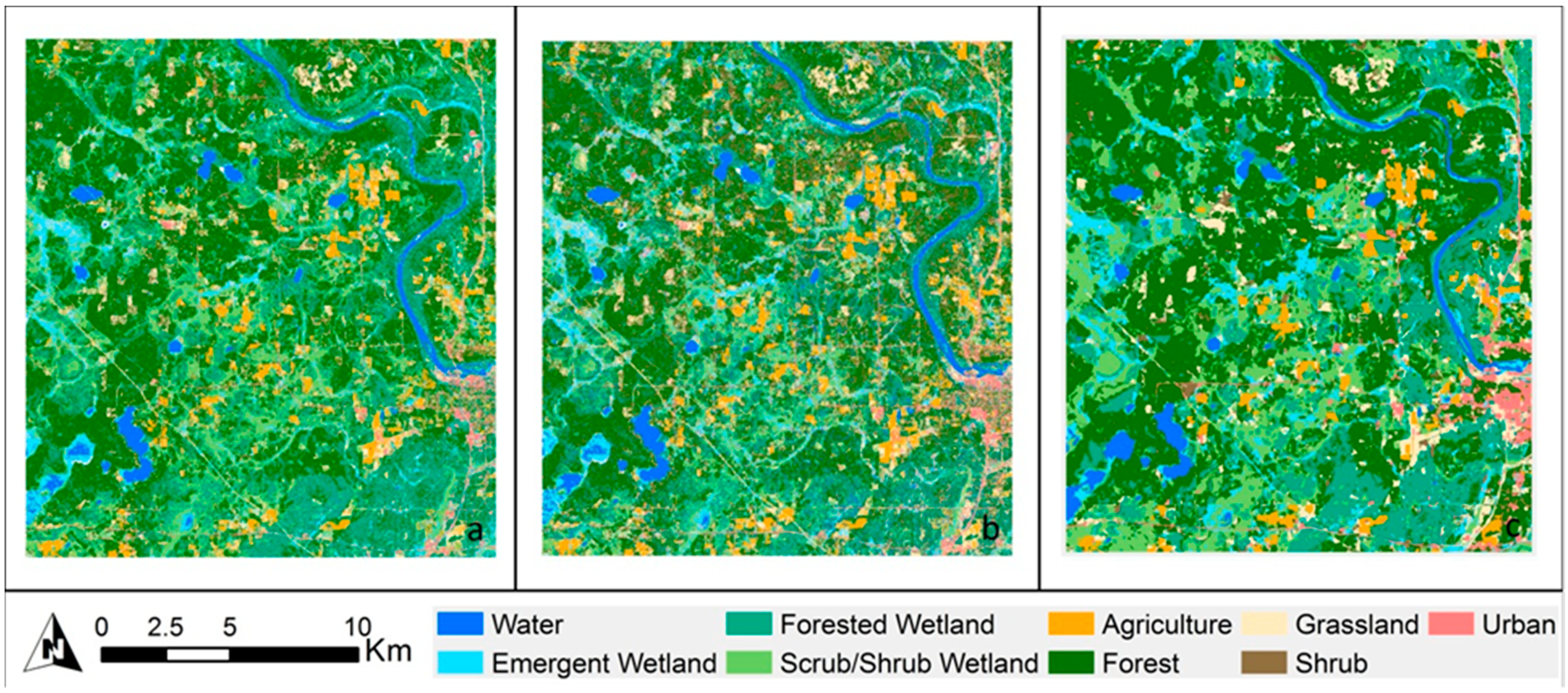
2.1.1. Cloquet
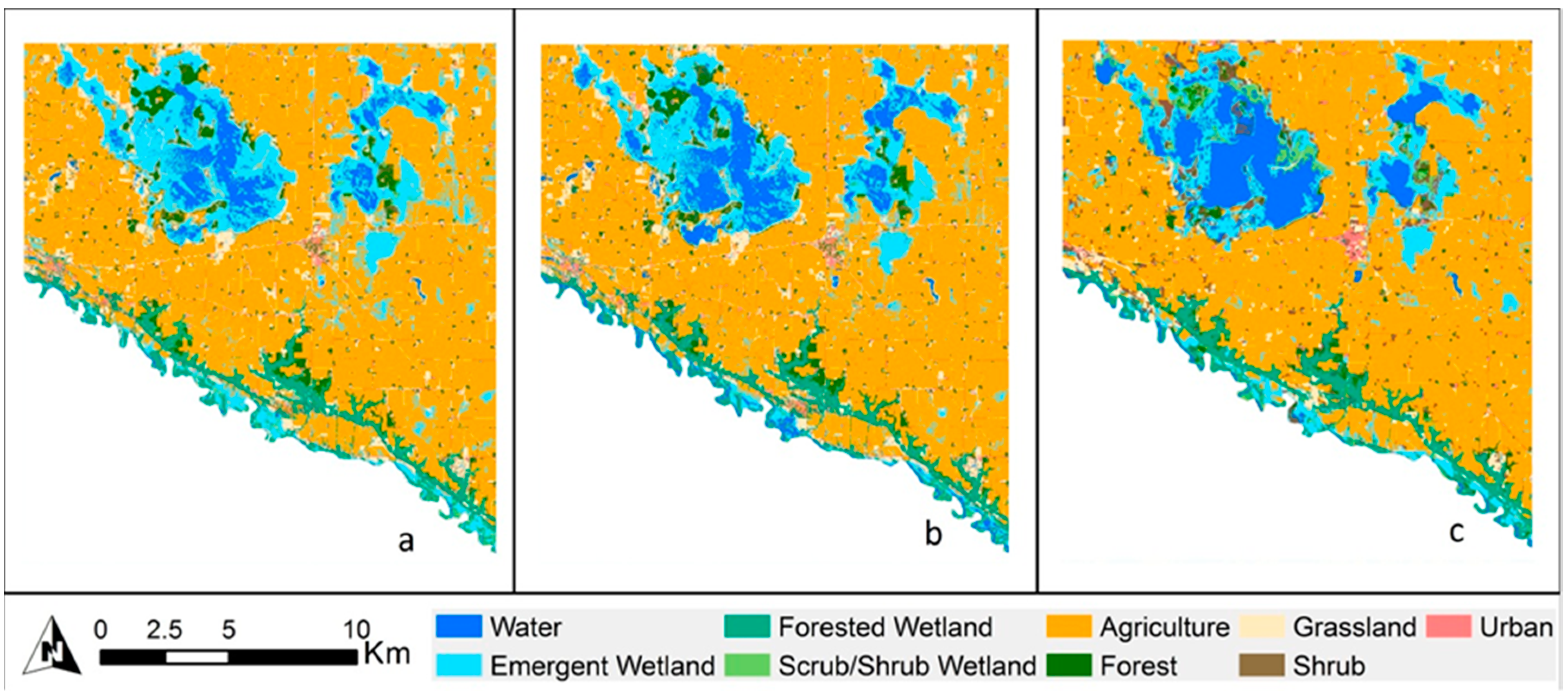
2.1.2. Mankato

2.2. Input Datasets and Process Flow
2.2.1. LiDAR-Derived Input Data
2.2.2. Optical Input Data
2.3. Land Cover Classification Schemes
2.4. Random Forest Classification
2.5. Training and Reference Data

| Land Cover Classification | Training Sites | Testing Sites | Final Total |
|---|---|---|---|
| Upland | 296 | 132 | 428 |
| Water | 48 | 18 | 66 |
| Wetland | 401 | 146 | 547 |
| Total | 745 | 296 | 1041 |
| Agriculture | 25 | 14 | 39 |
| Forest | 145 | 79 | 224 |
| Grassland | 53 | 12 | 65 |
| Shrub | 40 | 15 | 55 |
| Urban | 33 | 12 | 45 |
| Total | 296 | 132 | 428 |
| Emergent Wetland | 108 | 40 | 148 |
| Forested Wetland | 140 | 49 | 189 |
| Scrub/Shrub Wetland | 153 | 57 | 210 |
| Total | 401 | 146 | 547 |
| Land Cover Classification | Training Sites | Testing Sites | Final Total |
|---|---|---|---|
| Upland | 191 | 64 | 255 |
| Water | 24 | 8 | 32 |
| Wetland | 125 | 41 | 166 |
| Total | 340 | 113 | 453 |
| Agriculture | 71 | 24 | 95 |
| Forest | 24 | 8 | 32 |
| Grassland | 24 | 8 | 32 |
| Shrub | 28 | 9 | 37 |
| Urban | 44 | 15 | 59 |
| Total | 191 | 64 | 255 |
| Emergent Wetland | 63 | 21 | 84 |
| Forested Wetland | 49 | 16 | 65 |
| Scrub/Shrub Wetland | 13 | 4 | 17 |
| Total | 125 | 41 | 166 |
2.5.1. Point Training Data
2.5.2. Buffer Area Training Data
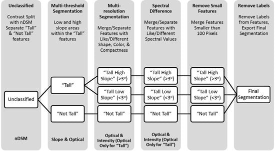
2.5.3. Image Object Area Training Data

2.6. Accuracy Assessment
3. Results
3.1. Classification Level 1
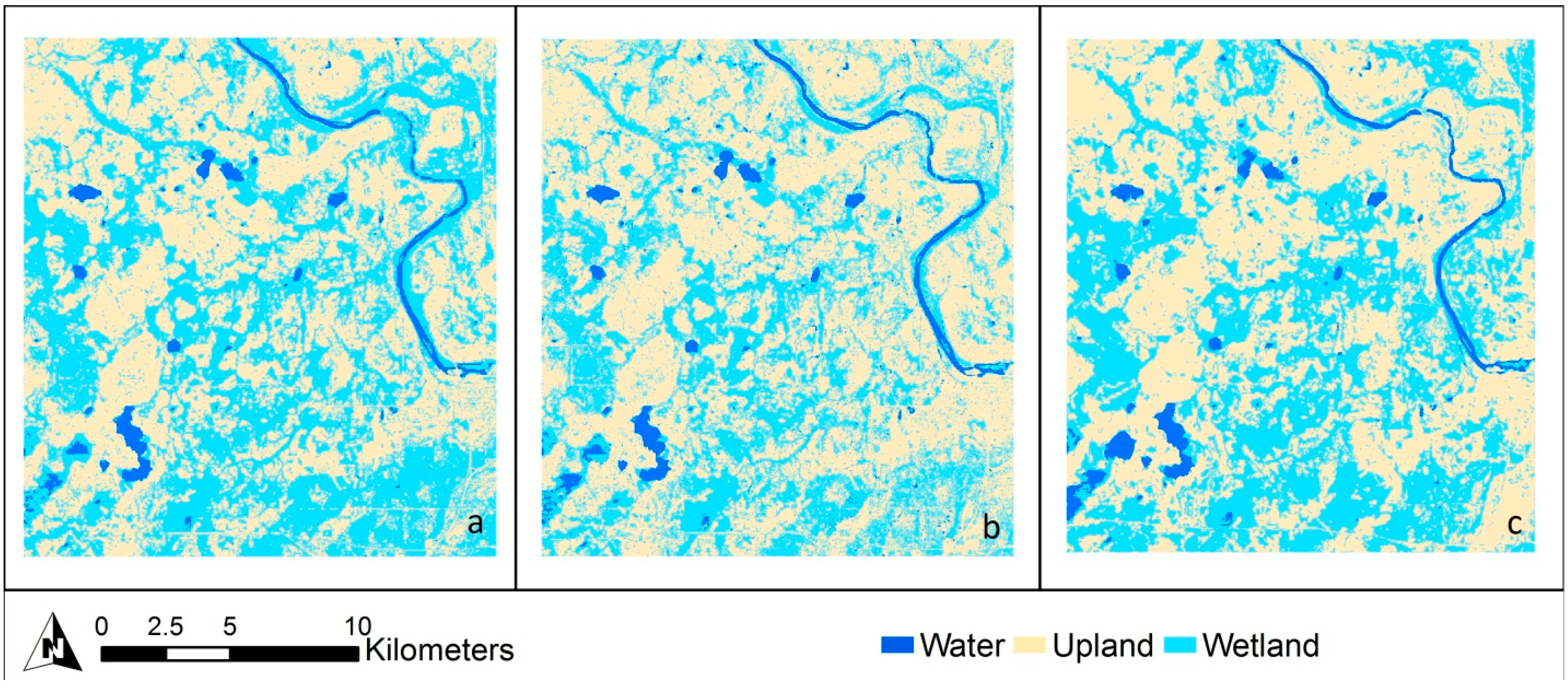
3.1.1. Cloquet

| Point Training | Buffer Area Training | Object Area Training | ||||
|---|---|---|---|---|---|---|
| Class | Producer’s Accuracy | User’s Accuracy | Producer’s Accuracy | User’s Accuracy | Producer’s Accuracy | User’s Accuracy |
| Water | 88 | 83 | 68 | 88 | 100 | 100 |
| Upland | 84 | 72 | 79 | 78 | 90 | 77 |
| Wetland | 76 | 85 | 79 | 77 | 81 | 93 |
| Overall Accuracy (%) | 80 (±5%) | 78 (±5%) | 86 * (±4%) | |||
| Kappa Statistic | 0.63 | 0.61 | 0.75 | |||
| Z Statistic | 14.5 * | 13.9 * | 50.5 * | |||
| Point Training | Buffer Area Training | Object Area Training |
|---|---|---|
| CTI | CTI | CTI—Mean |
| Green Band | Z Deviation | Green Band—Mean |
| Z Mean | Green Band | Z Deviation—Mean |
| Z Max | Blue Band | Z minimum—SD |
| Red Band | Z Maximum | NIR Band—Mean |
| Z Deviation | NIR Band | Intensity Min—Mean |
| Z Minimum | Red Band | Green Band—Max |
| Intensity Deviation | Intensity Deviation | Intensity Deviation—Mean |
| Blue Band | Z Mean | Z Mean—SD |
| Intensity Minimum | Z minimum | CTI—Mean |
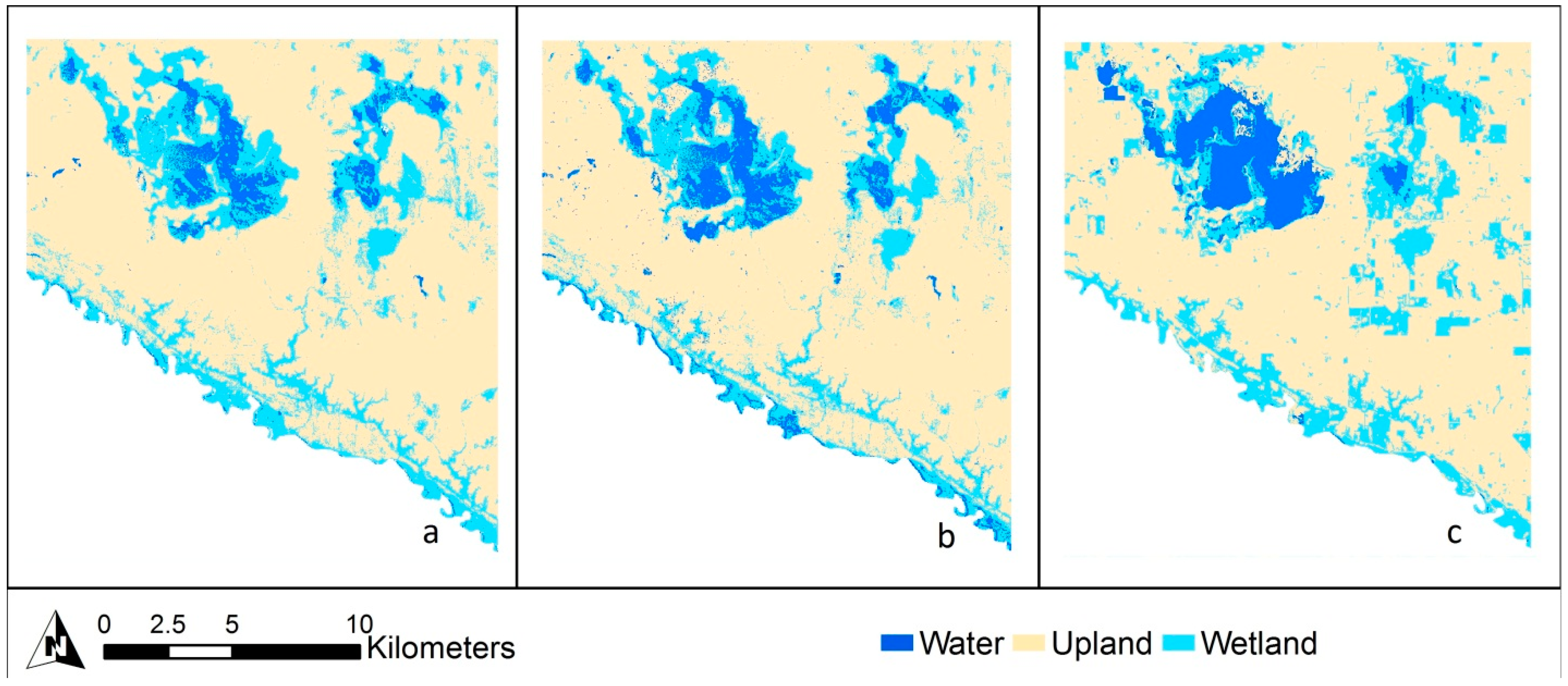
3.1.2. Mankato

| Point Training | Buffer Area Training | Object Area Training | ||||
|---|---|---|---|---|---|---|
| Class | Producer’s Accuracy | User’s Accuracy | Producer’s Accuracy | User’s Accuracy | Producer’s Accuracy | User’s Accuracy |
| Water | 100 | 100 | 80 | 100 | 80 | 100 |
| Upland | 97 | 97 | 97 | 97 | 100 | 97 |
| Wetland | 95 | 95 | 95 | 90 | 95 | 95 |
| Overall Accuracy (%) | 96 (±3%) | 95 (±4%) | 96.0 (±3%) | |||
| Kappa Statistic | 0.9 | 0.9 | 0.9 | |||
| Z Statistic | 29.0 * | 23.6 * | 29.9 * | |||
| Point Training | Buffer Area Training | Object Area Training |
|---|---|---|
| Z minimum | Z Minimum | Z Minimum—Max |
| CTI | CTI | CTI—Mean |
| Z Mean | Z Mean | Z Minimum—SD |
| Z Deviation | Green Band | Z Minimum—Mean |
| Green Band | Blue Band | Z Minimum—Min |
| Z Maximum | Intensity Minimum | Z Maximum—SD |
| Intensity Deviation | Intensity Deviation | Z Maximum—Min |
| Intensity Mean | Z Deviation | Intensity Maximum—SD |
| Intensity Minimum | Z Maximum | CTI—Min |
| Blue Band | Red Band | Z Mean—Mean |
3.2. Classification Level 2
3.2.1. Cloquet

| Point Training | Buffer Area Training | Object Area Training | ||||
|---|---|---|---|---|---|---|
| Class | Producer’s Accuracy | User’s Accuracy | Producer’s Accuracy | User’s Accuracy | Producer’s Accuracy | User’s Accuracy |
| Water | 67 | 89 | 67 | 89 | 100 | 100 |
| Emergent | 39 | 26 | 39 | 26 | 88 | 88 |
| Forested | 59 | 56 | 59 | 56 | 61 | 71 |
| Scrub/Shrub | 44 | 55 | 44 | 55 | 68 | 82 |
| Agriculture | 69 | 64 | 69 | 64 | 80 | 86 |
| Forest | 78 | 73 | 78 | 73 | 84 | 75 |
| Grassland | 31 | 42 | 31 | 42 | 70 | 58 |
| Shrub | 14 | 8 | 14 | 8 | 40 | 14 |
| Urban | 69 | 82 | 69 | 82 | 100 | 92 |
| Overall Accuracy (%) | 57 (±6%) | 57 (±6%) | 77 (±5%) | |||
| Kappa Statistic | 0.49 | 0.49 | 0.72 | |||
| Z Statistic | 13.8 * | 13.8 * | 24.2 * | |||
| Point Training | Buffer Area Training | Object Area Training |
|---|---|---|
| Z Deviation | Z Deviation | Z Deviation—Mean |
| nDSM | nDSM Slope | Intensity Min—Mean |
| Intensity Mean | Intensity Minimum | Z Mean—SD |
| nDSM Slope | nDSM | Intensity Min—SD |
| NDVI | Intensity Mean | Green Band—Mean |
| DEM | Z Maximum | nDSM Slope—Mean |
| Intensity Minimum | Red Band | Blue Band—Mean |
| Z Maximum | NIR Band | Z Deviation—Max |
| Red Band | Intensity Deviation | Red Band—Mean |
| Intensity Deviation | Blue Band | Intensity Deviation—Mean |
3.2.2. Mankato
| Point Training | Buffer Area Training | Object Area Training | ||||
|---|---|---|---|---|---|---|
| Class | Producer’s Accuracy | User’s Accuracy | Producer’s Accuracy | User’s Accuracy | Producer’s Accuracy | User’s Accuracy |
| Water | 100 | 100 | 80 | 100 | 80 | 100 |
| Emergent | 95 | 95 | 95 | 90 | 100 | 90 |
| Forested | 83 | 94 | 94 | 94 | 84 | 100 |
| Scrub/Shrub | 50 | 25 | 67 | 50 | 67 | 50 |
| Agriculture | 96 | 96 | 96 | 92 | 96 | 100 |
| Forest | 67 | 75 | 60 | 75 | 100 | 88 |
| Grassland | 64 | 88 | 64 | 88 | 100 | 75 |
| Shrub | 83 | 56 | 75 | 38 | 89 | 89 |
| Urban | 100 | 93 | 93 | 93 | 100 | 100 |
| Overall Accuracy (%) | 89 (±6%) | 88 (±7%) | 93 (±5%) | |||
| Kappa Statistic | 0.86 | 0.83 | 0.92 | |||
| Z Statistic | 13.8 * | 13.8 * | 24.2 * | |||

| Point Training | Buffer Area Training | Object Area Training |
|---|---|---|
| nDSM Slope | nDSM Slope | nDSM—Mean |
| NDVI | Blue Band | NDVI—Mean |
| Z Deviation | Z Deviation | nDSM—Minimum |
| Intensity Minimum | NDVI | NDVI—SD |
| DEM | Slope | nDSM—SD |
| Z Minimum | Green Band | Slope—Mean |
| Blue Band | DEM | CTI—Mean |
| Z Maximum | Intensity Maximum | Slope—SD |
| Intensity Deviation | Intensity Minimum | CTI—Minimum |
| nDSM | Intensity Deviation | Slope—Minimum |
4. Discussion
4.1. Cloquet
4.2. Mankato
5. Conclusions
Acknowledgments
Author Contributions
Conflicts of Interest
References
- Deschamps, A.; Greenlee, D.; Pultz, T.J.; Saper, R. Geospatial data integration for applications in flood prediction and management in the red river basin. In Proceedings of the IEEE International Geoscience and Remote Sensing Symposium and the 24th Canadian Symposium on Remote Sensing, Toronto, ON, Canada, 24–28 June 2002; pp. 3338–3340.
- Hodgson, M.; Jensen, J.; Mackey, H.; Coulter, M. Remote sensing of wetland habitat: A wood stork example. Photogramm. Eng. Remote Sens. 1987, 53, 1075–1080. [Google Scholar]
- Töyrä, J.; Pietroniro, A.; Martz, L.W.; Prowse, T.D. A multi-sensor approach to wetland flood monitoring. Hydrol. Process. 2002, 16, 1569–1581. [Google Scholar] [CrossRef]
- Vymazal, J. Constructed wetlands for wastewater treatment. Ecol. Eng. 2005, 25, 475–477. [Google Scholar] [CrossRef]
- Wissinger, S.A. Ecology of wetland invertebrates. In Invertebrates in Freshwater Wetlands of North America. Ecology and Management; Batzer, D.P., Rader, R.B., Wissinger, S.A., Eds.; Wiley: New York, NY, USA, 1999; pp. 1043–1086. [Google Scholar]
- Corcoran, J.M.; Knight, J.F.; Gallant, A.L. Influence of multi-source and multi-temporal remotely sensed and ancillary data on the accuracy of random forest classification of wetlands in Northern Minnesota. Remote Sens. 2013, 5, 3212–3238. [Google Scholar] [CrossRef]
- Rampi, L.P.; Knight, J.F.; Lenhart, C.F. Comparison of flow direction algorithms in the application of the CTI for mapping wetlands in Minnesota. Wetlands 2014, 34, 513–525. [Google Scholar] [CrossRef]
- Dahl, T.E.; Watmough, M.D. Current approaches to wetland status and trends monitoring in prairie Canada and the continental United States of America. Can. J. Remote Sens. 2007, 33, S17–S27. [Google Scholar] [CrossRef]
- Stout, D.J.; Kodis, M.; Wilen, B.O.; Dahl, T.E. Wetlands Layer—National Spatial Data Infrastructure: A Phased Approach to Completion and Modernization; US Fish and Wildlife: Washington, DC, USA, 2007.
- Corcoran, J.; Knight, J.; Brisco, B.; Kaya, S.; Cull, A.; Murnaghan, K. The integration of optical, topographic, and radar data for wetland mapping in northern Minnesota. Can. J. Remote Sens. 2011, 37, 564–582. [Google Scholar] [CrossRef]
- Ozesmi, S.L.; Bauer, M.E. Satellite remote sensing of wetlands. Wetl. Ecol. Manag. 2002, 10, 381–402. [Google Scholar] [CrossRef]
- Blaschke, T. Object based image analysis for remote sensing. ISPRS J. Photogramm. Remote Sens. 2010, 65, 2–16. [Google Scholar] [CrossRef]
- Steele, B.M.; Winne, J.C.; Redmond, R.L. Estimation and mapping of misclassification probabilities for thematic land cover maps. Remote Sens. Environ. 1996, 4257, 192–202. [Google Scholar]
- Rampi, L.P.; Knight, J.F.; Pelletier, K.C. Wetland mapping in the Upper Midwest United States: An object-based approach integrating LiDAR and imagery data. Photogramm. Eng. Remote Sens. 2014, 80, 439–449. [Google Scholar] [CrossRef]
- Lane, C.R.; D’Amico, E. Calculating the ecosystem service of water storage in isolated wetlands using LiDAR in North Central Florida, USA. Wetlands 2010, 30, 967–977. [Google Scholar] [CrossRef]
- Song, J.; Han, S.; Yu, K.; Kim, Y. Assessing the possibility of land-cover classification using LiDAR intensity data. Int. Arch. Photogramm. Remote Sens. Spat. Inf. Sci. 2002, 34, 259–262. [Google Scholar]
- Bwangoy, J.B.; Hansen, M.C.; Roy, D.P.; Grandi, G.D.; Justice, C.O. Wetland mapping in the Congo Basin using optical and radar remotely sensed data and derived topographical indices. Remote Sens. Environ. 2010, 114, 73–86. [Google Scholar] [CrossRef]
- Moore, I.; Grayson, R.; Landson, A. Digital terrain modeling: A review of hydrological, geomorphological, and biological applications. Hydrol. Process. 1991, 5, 3–30. [Google Scholar] [CrossRef]
- Knight, J.F.; Tolcser, B.; Corcoran, J.; Rampi, L. The effects of data selection and thematic detail on the accuracy of high spatial resolution wetland classifications. Photogramm. Eng. Remote Sens. 2013, 79, 613–623. [Google Scholar] [CrossRef]
- Chust, G.; Galparsoro, I.; Borja, Á.; Franco, J.; Uriarte, A. Coastal and estuarine habitat mapping, using LiDAR height and intensity and multi-spectral imagery. Estuar. Coast. Shelf Sci. 2008, 78, 633–643. [Google Scholar] [CrossRef]
- Collin, A.; Long, B.; Archambault, P. Salt-marsh characterization, zonation assessment and mapping through a dual-wavelength LiDAR. Remote Sens. Environ. 2010, 114, 520–530. [Google Scholar] [CrossRef]
- Lang, M.W.; McCarty, G.W. LiDAR intensity for improved detection of inundation below the forest canopy. Wetlands 2009, 29, 1166–1178. [Google Scholar] [CrossRef]
- Donoghue, D.N.M.; Watt, P.J.; Cox, N.J.; Wilson, J. Remote sensing of species mixtures in conifer plantations using LiDAR height and intensity data. Remote Sens. Environ. 2007, 110, 509–522. [Google Scholar] [CrossRef]
- Rodhe, A.; Seibert, J. Wetland occurrence in relation to topography—A test of topographic indices as moisture indicators. Agric. For. Meteorol. 1999, 98–99, 325–340. [Google Scholar] [CrossRef]
- Minnesota Department of Natural Resources. a Ecological classification system. Available online: http://www.dnr.state.mn.us/snas/naturalhistory.html (accessed on 20 August 2012).
- Minnesota Department of Natural Resources. b Wetlands Status and Trends. Available online: http://www.dnr.state.mn.us/eco/wetlands/wstm_prog.html. (accessed on 20 August 2012).
- Minnesota Department of Natural Resources. c State climatology office, MN climatology working group historical climate data. Available online: http://climate.umn.edu/doc/historical.htm (accessed on 20 August 2012).
- Mayer, A.L.; Lopez, R.D. Use of remote sensing to support forest and wetlands policies in the USA. Remote Sens. 2011, 3, 1211–1233. [Google Scholar] [CrossRef]
- Wang, L.; Liu, H. An efficient method for identifying and filling surface depressions in digital elevation models for hydrologic analysis and modelling. Int. J. Geogr. Inf. Sci. 2006, 20, 193–213. [Google Scholar] [CrossRef]
- Seibert, J.; McGlynn, B. A new triangular multiple flow-direction algorithm for computing upslope areas from gridded digital elevation models. Water Resour. Res. 2007, 43. [Google Scholar] [CrossRef]
- Gilmore, M.; Wilson, E.; Barrett, N.; Civco, D.; Prisloe, S.; Hurd, J.; Cary, C. Integrating multi-temporal spectral and structural information to map wetland vegetation in a lower Connecticut River tidal marsh. Remote Sens. Environ. 2008, 112, 4048–4060. [Google Scholar] [CrossRef]
- Cowardin, L.; Carter, V.; Golet, F.; LaRoe, E. Classification of Wetlands and Deepwater Habitats of the United States; U.S. Department of the Interior, Fish and Wildlife Service: Washington, DC, USA, 1979; p. 79.
- Breiman, L. Random forests. Mach. Learn. 2001, 45, 5–32. [Google Scholar] [CrossRef]
- Castañeda, C.; Ducrot, D. Land cover mapping of wetland areas in an agricultural landscape using SAR and Landsat imagery. J. Environ. Manag. 2009, 90, 2270–2277. [Google Scholar] [CrossRef]
- Parmuchi, M.G.; Karszenbaum, H.; Kandus, P. Mapping wetlands using multi-temporal RADARSAT-1 data and a decision-based classifier. Can. J. Remote Sens. 2002, 28, 175–186. [Google Scholar] [CrossRef]
- Yuan, F.; Sawaya, K.E.; Loeffelholz, B.C.; Bauer, M.E. Land cover classification and change analysis of the Twin Cities (Minnesota) Metropolitan Area by multitemporal Landsat remote sensing. Remote Sens. Environ. 2005, 98, 317–328. [Google Scholar] [CrossRef]
- Ketting, R.L.; Landgrebe, D.A. Classification of multispectral image data by extraction and classification of homogeneous objects. IEEE Trans. Geosci. Remote Sens. 1976, 14, 19–26. [Google Scholar] [CrossRef]
- Haralick, R.; Shapiro, L. Survey: Image segmentation techniques. Comput. Vis. Graph. Image Process. 1985, 29, 100–132. [Google Scholar] [CrossRef]
- Hay, G.; Marceau, D.; Dube, P.; Bouchard, A. A multiscale framework for landscape analysis: Object-specific analysis and upscaling. Landsc. Ecol. 2001, 16, 471–490. [Google Scholar] [CrossRef]
- Kartikeyan, B.; Sarkar, A.; Majumder, K. A segmentation approach to classification of remote sensing imagery. Int. J. Remote Sens. 1998, 19, 1695–1709. [Google Scholar] [CrossRef]
- Pal, R.; Pal, K. A review on image segmentation techniques. Pattern Recognit. 1993, 26, 1277–1294. [Google Scholar] [CrossRef]
- Benz, U.C.; Hofmann, P.; Willhauck, G.; Lingenfelder, I.; Heynen, M. Multi-resolution, object-oriented fuzzy analysis of remote sensing data for GIS-ready information. ISPRS J. Photogramm. Remote Sens. 2004, 58, 239–258. [Google Scholar] [CrossRef]
- Hay, G.; Castilla, G.; Wulder, M.; Ruiz, J. An automated object based approach for the multiscale image segmentation of forest scenes. Int. J. Appl. Earth Obs. Geoinf. 2005, 7, 339–359. [Google Scholar] [CrossRef]
- Nobrega, R.A.; O’Hara, C.G.; Quintanilha, J.A. An object-based approach to detect road features for informal settlements near Sao Paulo, Brazil. In Object Based Image Analysis; Springer: Heidelberg/Berlin, Germany, 2008; pp. 589–607. [Google Scholar]
- O’Neil-Dunne, J.P.M.; MacFaden, S.W.; Royar, A.R.; Pelletier, K.C. An object-based system for LiDAR data fusion and feature extraction. Geocarto Int. 2013, 28, 227–242. [Google Scholar] [CrossRef]
- Whitcomb, J.; Moghaddam, M.; McDonald, K.; Kellndorfer, J.; Podest, E. Mapping vegetated wetlands of Alaska using L-band radar satellite imagery. Can. J. Remote Sens. 2009, 35, 54–72. [Google Scholar] [CrossRef]
- Congalton, R.; Green, K. (Eds.) Assessing the Accuracy of Remotely Sensed Data: Principles and Practices, 2nd ed.; CRC Press: Boca Raton, FL, USA, 2008; p. 200.
© 2015 by the authors; licensee MDPI, Basel, Switzerland. This article is an open access article distributed under the terms and conditions of the Creative Commons Attribution license (http://creativecommons.org/licenses/by/4.0/).
Share and Cite
Corcoran, J.; Knight, J.; Pelletier, K.; Rampi, L.; Wang, Y. The Effects of Point or Polygon Based Training Data on RandomForest Classification Accuracy of Wetlands. Remote Sens. 2015, 7, 4002-4025. https://doi.org/10.3390/rs70404002
Corcoran J, Knight J, Pelletier K, Rampi L, Wang Y. The Effects of Point or Polygon Based Training Data on RandomForest Classification Accuracy of Wetlands. Remote Sensing. 2015; 7(4):4002-4025. https://doi.org/10.3390/rs70404002
Chicago/Turabian StyleCorcoran, Jennifer, Joseph Knight, Keith Pelletier, Lian Rampi, and Yan Wang. 2015. "The Effects of Point or Polygon Based Training Data on RandomForest Classification Accuracy of Wetlands" Remote Sensing 7, no. 4: 4002-4025. https://doi.org/10.3390/rs70404002