1. Introduction
Aerosol extinction is a good measure in LiDAR applications to evaluate the aerosol characteristics, as the light extinction from aerosol is due to the dependence of light scattering and absorption on the aerosol size, shape, chemical composition and density [
1,
2]. Elastic backscatter LiDAR has proven to be a powerful tool in remote sensing of aerosol characteristics [
3]. With the advantages of high spatial and temporal resolution, a large dynamic range and continuous observing, more and more backscatter LiDAR systems have been employed for aerosol research [
4,
5,
6]. The European Aerosol Research LiDAR Network has made good contributions to the collection of quantitative, comprehensive and statistical data for the temporal distribution of aerosols on a continental scale over Europe since 2000 [
7,
8]. However, aerosol extinction cannot be derived directly from elastic backscatter LiDARs, as the assumption of the LiDAR ratio (aerosol extinction for aerosol backscatter coefficients) is needed in the retrieval procedure [
9,
10], which produces considerable uncertainties for the final products. Raman LiDAR and high spectral resolution LiDAR are good solutions for the precise detection of aerosol extinction without any assumptions [
11,
12]. However, their implementation is more complex and expensive, which limits their application to a large scope. In addition, vertical profiles from elastic backscatter LiDAR suffer from the existence of an overlap function [
13,
14], which affects its probing in the near-filed atmosphere, especially in the study of the atmospheric boundary layer.
Scanning mode is a special working condition for LiDAR systems [
15,
16,
17]. It can provide atmospheric information in the profile with a fixed angle, as well as two-dimensional (2D) spatial scans (range-height-indicator (RHI) scan or plane-position-indicator scan), which give LiDAR remote sensing the capability to map atmospheric parameters [
18,
19]. For the application of scanning elastic backscatter LiDAR, the multiangle method is investigated to retrieve the vertical profile of atmospheric optical properties without the assumption of a relationship between extinction and backscatter coefficients [
15,
20]. The critical requirement in the multiangle method is the horizontally homogeneous particle backscatter and extinction coefficients at all measurement heights, which are often not fulfilled. In order to improve the retrieval procedure by using scanning elastic backscatter LiDAR, many efforts, including performance analysis of the scanning LiDAR, as well as the modified retrieval method, have been made recently [
21,
22,
23].
The University of Nova Gorica built a long-range ultraviolet scanning elastic backscatter LiDAR at Otlica observatory (45.93°N, 13.91°E, elevation 945 m above sea level), which has the capability to study atmospheric processes over the southwest region of Slovenia [
24,
25]. Aerosol extinction is retrieved after scanning measurement by using the multiangle method, which can be taken as an average result in the scanning region. Moreover, air flow trajectories from Hybrid Single Particle Lagrangian Integrated Trajectory Model (HYSPLIT) were modeled to analyze the sources of the aerosols and their effects on the local environment. Data processing procedures of the scanning LiDAR are presented in the paper in detail, which can be used in most scanning elastic backscatter LiDAR by using the multiangle retrieval method for the measurement of atmospheric variables.
2. LiDAR System and Its Experimental Setup
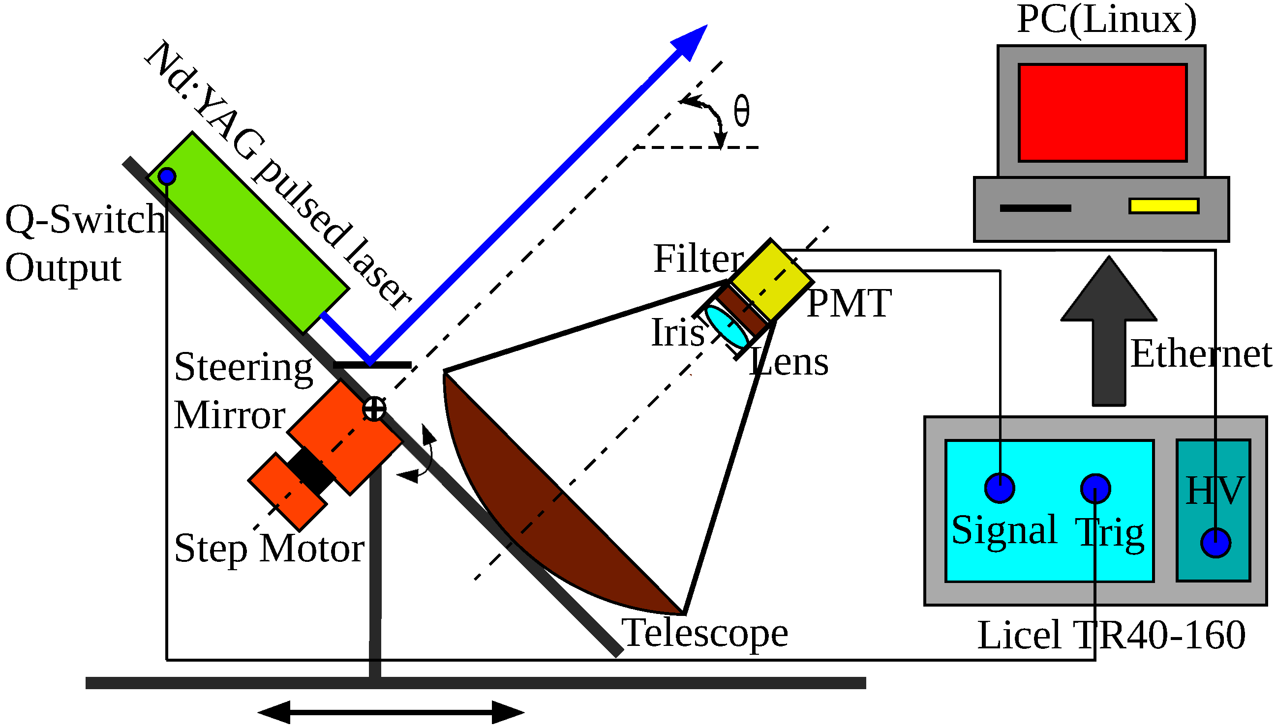
A schematic diagram of the ultraviolet scanning elastic backscatter LiDAR system is shown in
Figure 1. A high power compact Q-switched Nd:YAG pulsed laser is employed as the transmitter, which produces a laser pulse with an energy of 95 mJ per pulse at 355 nm after triple frequency. A parabolic mirror with a diameter of 800 mm and a focal length of 410 mm is utilized as the receiver. Both the transmitter and receiver are mounted on a common frame to make the LiDAR system steerable, but only with the elevation angle changing from −5° to 90°. The offset of the laser beam direction has been calibrated against a self-leveling laser to improve the performance of the LiDAR system [
26]. A photomultiplier tube (PMT) is positioned near the focus of the parabolic mirror to detect the LiDAR return signals. In order to suppress the background components in the total backscattering light, an iris, a collimating lens and an interference filter are put consequently in front of the PMT. With the current filter, background noise in daytime operation is still prohibitive, thus all of the measurements are performed during the night. The output of the PMT is amplified and digitized by a Licel TR40-160 transient recorder, which is connected to a Linux-based data acquisition computer via an Ethernet link. The data acquisition software based on C++ code and the ROOT package features graphical interfaces for the full digitizer, laser and telescope control and physics analysis. The detailed specifications of the scanning LiDAR are listed in
Table 1.
Figure 1.
Schematic diagram of the scanning elastic backscatter LiDAR system. The direction of the LiDAR in the elevation angle θ can be changed from −5° to 90°, while the azimuth angle is fixed. The axis of rotation for the elevation angle scanning is denoted by ⊕.
Figure 1.
Schematic diagram of the scanning elastic backscatter LiDAR system. The direction of the LiDAR in the elevation angle θ can be changed from −5° to 90°, while the azimuth angle is fixed. The axis of rotation for the elevation angle scanning is denoted by ⊕.
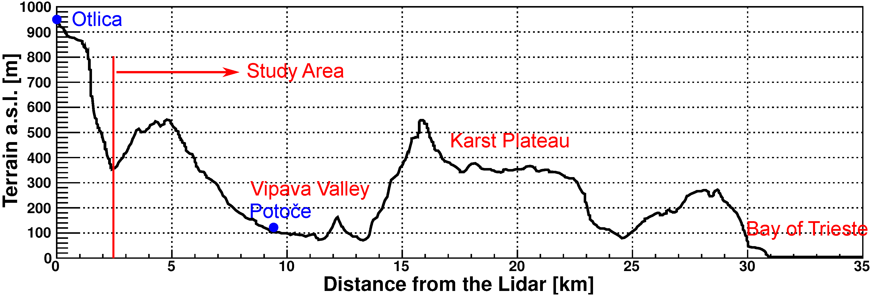
The measurement parameters of scanning LiDAR are set to consider the measured objects (
Figure 2) and time scale of atmospheric turbulence [
27]. The atmosphere from the LiDAR site to the Bay of Trieste with a distance of about 30 km is our study interest, which covers the Vipava Valley and the Karst Plateau. In our case, the LiDAR was set to scan the vertical atmosphere between elevation angles of −4° and 20°. The lowest elevation angle of −4° was set to consider the influences of the altitude of LiDAR site and the non-obscured LiDAR view. The angular step was set to 0.5° to increase the extraction of atmospheric information of interest. At each step, 200 laser shots were recorded, averaged and stored in a binary ROOT file. Simultaneously-obtained analog data and photon counting data by the Licel transient recorder were merged to make the data uniform and to improve the detection range, as well as signal-to-noise ratio (SNR) [
26].
Table 1.
Specifications of the scanning elastic backscatter LiDAR systems. PMT, photomultiplier tube.
Table 1.
Specifications of the scanning elastic backscatter LiDAR systems. PMT, photomultiplier tube.
| Transmitter | Quantel Brilliant B |
| Wavelength/pulse energy | 355 nm/95 mJ |
| Repetition rate/pulse width | 20 Hz/7 ns |
| Receive | Parabolic mirror |
| Diameter/focal length | 800 mm/410 mm |
| Filter | Barr Associates Inc. |
| Central wavelength/bandwidth | 355 nm/5 nm |
| Detector | Hamamatsu PMT R7400 |
| Voltage | 770 V |
| Data acquisition | Licel TR40-160 |
| Analog A/D resolution/sampling rate | 12 bit/40 Ms/s |
| PC max. count rate/temporal resolution | 250 MHz/25 ns |
| Memory length/range resolution | 16,380/3.75 m |
Figure 2.
Terrain configuration along the LiDAR scanning line. The study area is marked by the red arrow, including the Vipava Valley, the Karst Plateau and the Bay of Trieste. In order to see the variation of the terrain configuration in the study area, the vertical axis is scaled in meters, while the horizontal axis of the distance from the LiDAR is scaled in kilometers.
3. Multiangle Retrieval Method of Aerosol Optical Variables
Considering both the aerosol and molecular contributions in the volume extinction coefficient
α(
r) and volume backscatter coefficient
β(
r), the scanning elastic backscatter LiDAR equation can be rewritten as:
where
P (
r) is the instantaneous received power,
C the LiDAR system constant, including the losses in optics and effective receiver aperture, and
P0 the transmitted laser power. The scanning LiDAR equation is thus parameterized with the range
r (along the path in which the transmitting laser pulse goes) and elevation angle
θ for describing atmospheric conditions.
Background noise
Pbg should be subtracted first in the data processing, as a small error estimate may result in a large offset bias in the range squared corrected signal (RSCS). It is estimated from the signals at the last 1000 bins of the trace [
28], which corresponds to the last 3.75 km within the whole detection range of 61.42 km. After denoising, the
S-function of the scanning elastic backscatter LiDAR can be written as:
where
c = ln(
CP0). In the horizontal invariant atmosphere, atmospheric variables are only changed with height
h (
h =
r · sin
θ). Thus, the range-dependent
S-function in a horizontal homogeneous atmosphere can be written in terms of the height
h and geometric factor
ξ = 1/ sin
θ = csc
θ as:
In the application of ultraviolet light, the molecular scattering should be considered, as the intensity of molecular scattering is inversely proportional to the forth power of the wavelength [
29]. With the purpose of retrieving aerosol properties only, corrections of Rayleigh scattering in the
S-function are necessary in the application of an ultraviolet LiDAR system. Therefore, we introduce a novel symbol
S′ to express the
S-function without molecular contribution on attenuation as:
Molecular optical depth along the height
can be estimated from the standard atmosphere model [
30] or co-located radiosonde data. Thus, aerosol optical depth (AOD) along the height
and the relative backscatter coefficient
c + ln [
βa(
h, ξ) +
βm(
h, ξ)] are defined as the slope and intercept of the resulting linear function
S′(
h, ξ) =
f(
h, ξ) in
ξ when
h is kept constant. Therefore, the AOD of the horizontally-invariant atmosphere at the fixed height can be calculated from the horizontal derivative of the
S′-function in the rows of the pixels of 2D spatial scans, while reconstruction of the backscatter coefficient needs the absolute value of LiDAR system constant
c, which is out of the scope of this study. The final product of aerosol extinction is then derived by doing differential calculation from the AOD side, as aerosol optical depth at a given height is an integral function of the aerosol extinction coefficient along the height [
9,
10].
4. Data Processing
In order to make the measurement data from the ultraviolet scanning LiDAR retrievable, a series of procedures need to be fulfilled by using the multiangle retrieval method of aerosol optical variables. Most of them are described in
Section 3. Besides, the calculation of SNR is performed to scale the detection range [
28]. Correction of Rayleigh scattering is done to minimize the influence of Rayleigh scattering of ultraviolet light on the retrieval of aerosol optical variables. The 2D RHI diagram is plotted to reconstruct the scan plot with a precision pixel coordinate in both axes. Assessment of horizontal atmospheric homogeneity is executed by evaluating the linearity of the extracted horizontal pixel data points from the 2D RHI diagram line with the distance from the LiDAR site. In the following, construction of the 2D RHI diagram, correction of the Rayleigh scattering, assessment of the horizontal atmospheric homogeneity and retrieval of the aerosol optical variables are described in detail.
Figure 3.
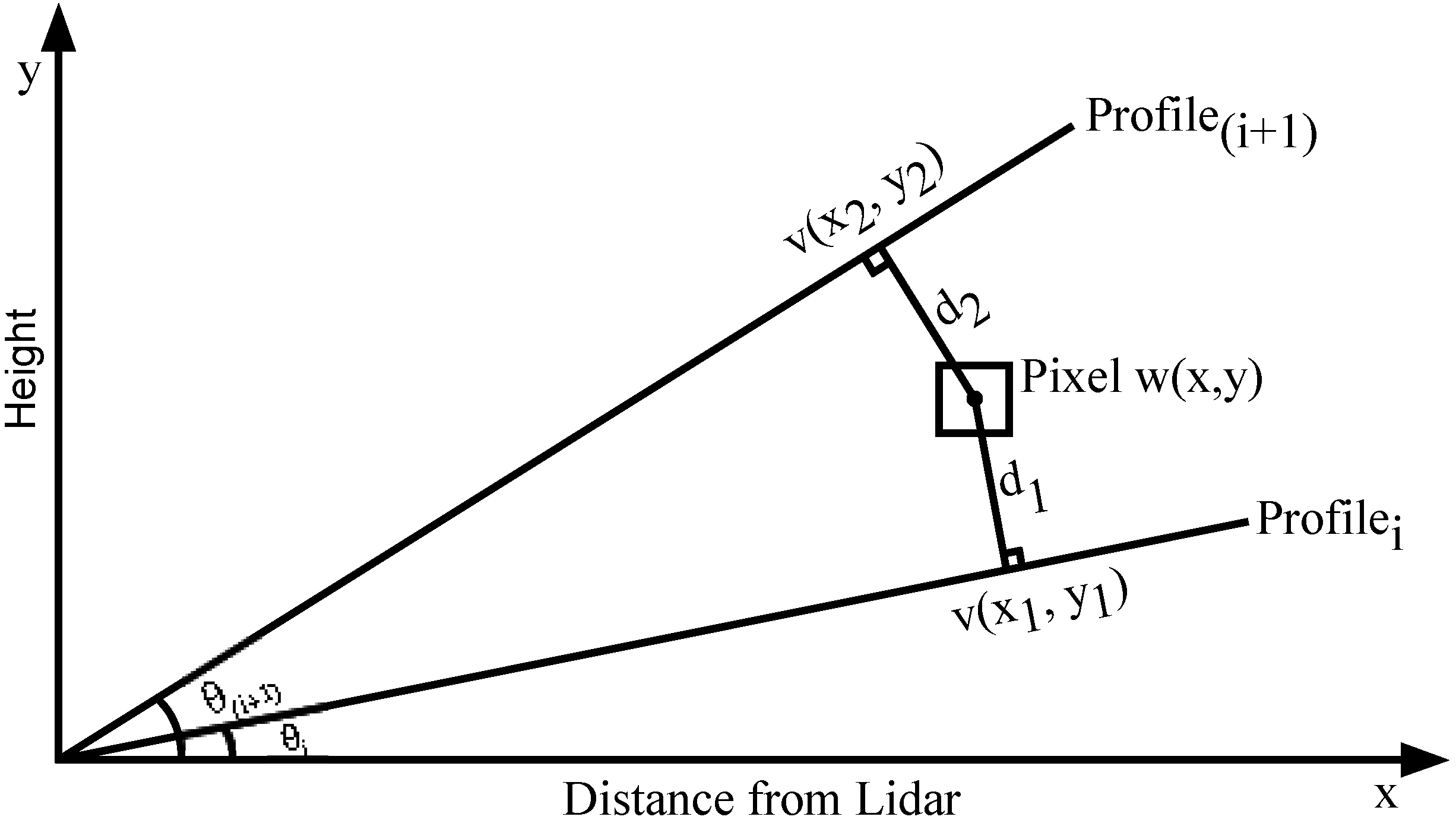
Construction of Cartesian 2D range-height-indicator (RHI) diagrams. A weighted logarithm range squared corrected signal (RSCS) value is calculated by a barycentric interpolation scheme between the LiDAR return signal profiles from successive scanning angles. Each pixel of the diagram represents atmospheric information at that position.
Figure 3.
Construction of Cartesian 2D range-height-indicator (RHI) diagrams. A weighted logarithm range squared corrected signal (RSCS) value is calculated by a barycentric interpolation scheme between the LiDAR return signal profiles from successive scanning angles. Each pixel of the diagram represents atmospheric information at that position.
4.1. Construction of the Range-Height-Indicator Diagram
The spatial distribution of the LiDAR return signal (logarithm RSCS) obtained by scanning is presented in Cartesian 2D RHI diagrams with a resolution of 50 m in both coordinates. The horizontal axis represents the distance from the LiDAR and the vertical axis the height relative to the altitude of the LiDAR site. Each Cartesian 2D RHI diagram is reconstructed from the profiles scanned at discrete elevation angles with an increment of 0.5°. To fill the pixels of the 2D RHI diagram, a weighted value of the logarithm RSCS is constructed by using a barycentric interpolation scheme [
31] between successive step profiles (
Figure 3). The weighted RSCS value
w(
x, y) at each pixel is calculated as:
where
v(
x1, y1) and
v(
x2, y2) are the measured logarithm RSCS values in successive step profiles.
d1 and
d2 are the shortest distances between the center coordinates of each pixel and the closest profiles on both sides.
Figure 4 is an example of the RHI diagram from the measurement result by the ultraviolet scanning elastic backscatter LiDAR, in which only the data with SNR ≥ 1 are filling in the pixels of the 2D RHI plot.
Figure 4.
Effect of Rayleigh correction (top, before; bottom, after) on a 2D RHI diagram to show the atmospheric conditions. The scan example was taken from the LiDAR-radiosonde measurements at 19:23 Central European Time (CET) on 12 October 2011. The height is given relative to the altitude of the LiDAR site.
4.2. Correction of Rayleigh Scattering
Rayleigh scattering is an elastic scattering of light radiation by molecules in the atmosphere, which are much smaller than or comparable to the wavelength of light. The intensity of molecular volume scattering coefficient
βm, which is the product of molecular cross-section
σm and molecular number density
Nm at the existing pressure and temperature, can be described as [
28]:
where
λ is the excited wavelength,
n the real part of the index of refraction and
Ns the number density of molecules at standard conditions (
Ns = 2.547 × 10
19 cm
3 at
Ts = 288.15 K and
Ps = 1013.25 hPa). Molecular cross-section
σm can be thought of as constant in the atmosphere, while molecular number density
Nm is a function of pressure and temperature, which are changed with height variation. Moreover, from the light scattering theory, molecular extinction and backscatter coefficients are related by the expression [
28]:
Therefore, after the estimation of molecular number density, molecular attenuation can be corrected by Equation (4).
Figure 4 shows the 2D RHI diagrams before and after the Rayleigh correction, in which only pixels with SNR ≥ 1 were filled. Although the pixel values filled with the logarithm RSCS in the 2D RHI diagram have small differences, we can distinguish the contour change between these two RHI diagrams, which shows the effects of Rayleigh correction on the
S-function.
4.3. Assessment of Horizontal Atmospheric Homogeneity
The critical requirement of the scanning elastic backscatter LiDAR in the application of the multiangle retrieval method is the horizontal homogeneous atmosphere. However, the aerosol distribution is affected by the natural conditions and human activities, which result in the existence of horizontal variant atmosphere. In our case, to apply the multiangle retrieval method described in
Section 3, the assumption of horizontal atmospheric homogeneity in the study region was made. The assumption feasibility was assessed by extracting the horizontal pixel data points from the 2D RHI diagram and investigating the linearity of the constructed line with the distance from the LiDAR site.
Figure 5.
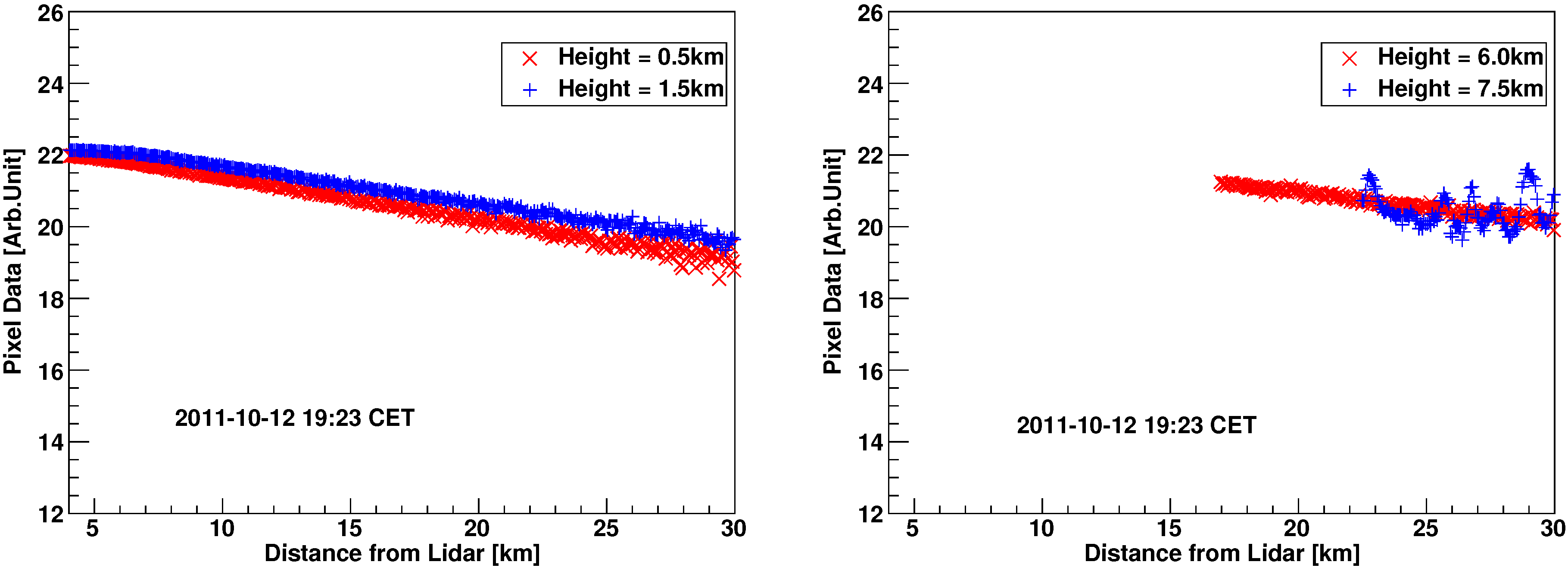
Examples of the horizontal pixel data extracted from the 2D RHI diagrams (
Figure 4). (
Left) At the heights of 0.5 km and 1.5 km; (
Right) at the heights of 6.0 km and 7.5 km. Height is given relative to the altitude of the LiDAR site.
Figure 5.
Examples of the horizontal pixel data extracted from the 2D RHI diagrams (
Figure 4). (
Left) At the heights of 0.5 km and 1.5 km; (
Right) at the heights of 6.0 km and 7.5 km. Height is given relative to the altitude of the LiDAR site.
Figure 5 shows the horizontal pixel data extracted from the 2D RHI diagram (
Figure 4, bottom) at the heights of 0.5 km, 1.5 km, 6.0 km and 7.5 km. From the plots, we can see that at the heights of 0.5 km, 1.5 km and 6.0 km, the horizontal pixel data with the weighted logarithm RSCS values form almost a straight line, justifying the assumption of horizontal atmospheric homogeneity at these heights in the study region. While the horizontal pixel data at the height of 7.5 km are loosely distributed, which was the result of the cloud turbulence (
Figure 4). Therefore, by examining the horizontal pixel data at all heights from the 2D RHI diagram, we can say that the assumption of a horizontal homogeneous atmosphere in the study region (
Figure 2) can be made up to the height of 6.0 km during this measurement section.
4.4. Retrieval of Aerosol Optical Variables
By definition, optical depth is a measure of the proportion of radiation absorbed or scattered along a path through a partially transparent medium. However, in the invariant atmosphere, aerosol optical properties are changed only with height. It is convenient to redefine optical depth in such a case, which can be regarded as the integration of light absorbed or scattered along the height. In this paper, the new definition of optical depth is employed.
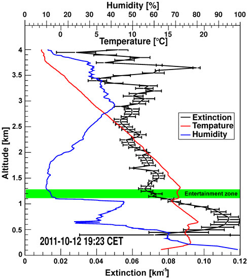
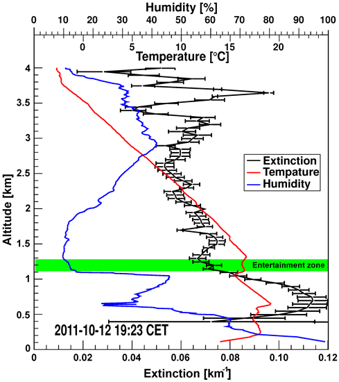
Figure 6.
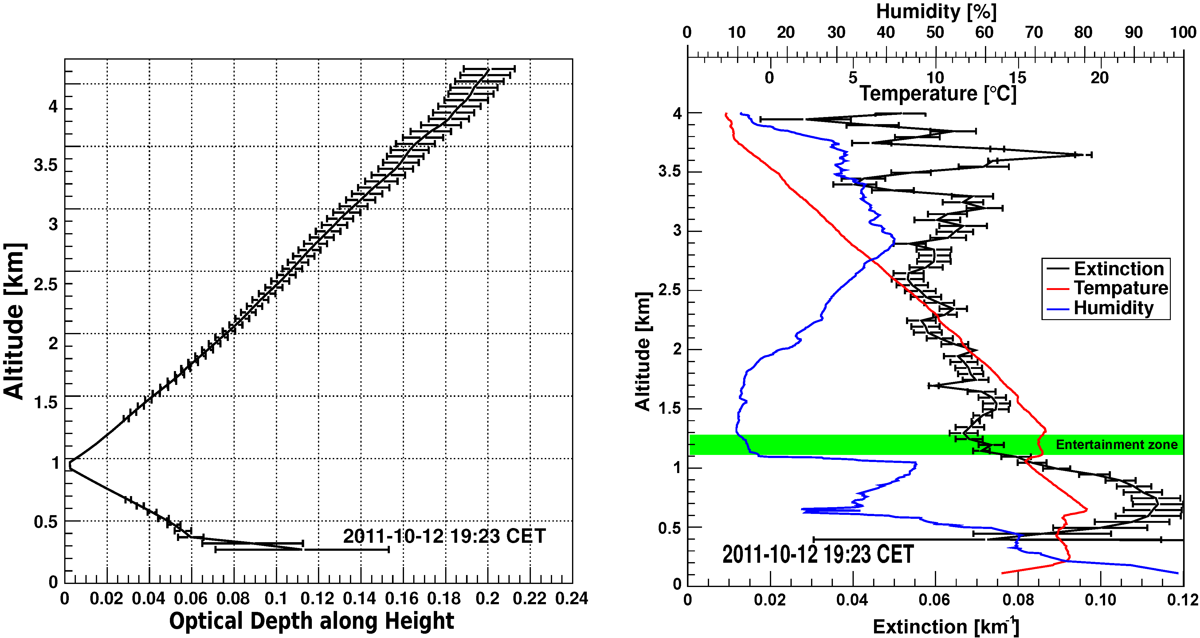
Retrieval results of the aerosol optical depth (
left) and aerosol extinction (
right) from the performed spatial scan on 12 October 2011 (
Figure 4, bottom). The simultaneously-obtained temperature and humidity profiles from radiosonde measurements at Potocˇe are shown for comparison and the determination of the atmospheric boundary layer height. The green bar shows the entertainment zone determined by the LiDAR and radiosonde joint measurements. Altitude is given relative to the vertical distance above the sea level.
Figure 6.
Retrieval results of the aerosol optical depth (
left) and aerosol extinction (
right) from the performed spatial scan on 12 October 2011 (
Figure 4, bottom). The simultaneously-obtained temperature and humidity profiles from radiosonde measurements at Potocˇe are shown for comparison and the determination of the atmospheric boundary layer height. The green bar shows the entertainment zone determined by the LiDAR and radiosonde joint measurements. Altitude is given relative to the vertical distance above the sea level.
In the application of the scanning elastic backscatter LiDAR, optical depth at a fixed height can be calculated from the horizontal derivative of the
S′-function (Equation (4)). With the credibility of horizontal atmospheric homogeneity, optical depth in the invariant atmosphere was calculated from the analysis of horizontal rows of pixels in the 2D RHI diagram (
Figure 6 (left)). Error bars represent uncertainties in the fitting of the
S′-function to the data. Errors increase linearly with height for geometrical and accumulation reasons. The results show that the optical depth value increases with height, which can be explained by the vertical LiDAR equation that optical depth at a given height is an integral of aerosol extinction from the LiDAR site (
h = 0) to the given height
h (relative to the LiDAR site). Therefore, the slope of the AOD profile expresses the variation of the average aerosol extinction within the height interval.
From their integration/differential relationship, aerosol extinction can be derived from AOD as:
Using this technique, aerosol extinction was calculated and presented in
Figure 6 (right). One or more obvious aerosol layers were observed in the profile. The atmospheric boundary layer (ABL) height can be determined from the position of the minimum of aerosol extinction by using the logarithm gradient method [
3,
24], which can be recognized at the height of 1.30 km in this scanning measurement case. Simultaneously, temperature and humidity profiles from the radiosonde measurements were plotted in
Figure 6 (right) as well, which was launched at Potocˇe, along the scanning line and in the middle of the detection range (far away, 9.2 km from the LiDAR site). Radiosonde measurements revealed that the temperature profile was not linearly decreasing and manifested a number of variations below 1.31 km, while relative humidity decreased rapidly at 1.07 km. These two altitudes defined the entrainment zone, where air masses from the free troposphere became incorporated into the ABL. The top of the radiosonde-obtained entrainment zone can be thought of as the ABL height and is characterized by the minimum in humidity distribution and the last big inversion in the temperature distribution. It agrees well with the ABL height obtained by the scanning LiDAR measurement.
5. Investigation of Aerosol Variability
From August to October in 2010, the scanning elastic backscatter LiDAR was used to investigate aerosol variability in the southwest of Slovenia. The statistical information regarding these measurements is summarized in
Table 2, which yields 28 days of LiDAR data. All of the measurements were performed after sunset between 20:00 CET and 03:00 + 1 CET. For the sake of statistics, the consecutive measurements during the same night were divided into those before 24:00 CET and those after 00:00 CET. The measurements performed after 00:00 CET were recorded as the data on the second day. The missing days were mainly due to bad weather and technical problems.
Table 2.
Statistics of the measurement days of LiDAR scanning measurements.
Table 2.
Statistics of the measurement days of LiDAR scanning measurements.
| Months | Performed Days | Day List |
|---|
| August 2010 | 10 | 16, 17∗, 19, 21, 22# , 26, 27, 29, 30 and 31∗ |
| September 2010 | 10 | 1, 2∗, 3, 10, 11∗, 12, 20, 21∗, 22 and 23 |
| October 2010 | 8 | 3, 7, 9# , 10, 11, 14, 15 and 21# |
As the existence of clouds makes the atmosphere turbulent, which is a disaster for the assumption of horizontal atmospheric homogeneity, all of the measurements were checked with the height of clouds present. Cloud coverage below 2 km in the study region was counted, considering that the ABL height in Europe is typically less than 2 km; thus, two classes were defined to distinguish the good measurements from bad measurements. Class I consists of all measurements containing no clouds below 2 km, which are named “cloud-free”. The aerosol extinction profile can be retrieved up to high altitudes in such cases. In Class II, cloud coverage at heights below 2 km was present during the scanning measurements. The statistics regarding these two classes in the performed measurements is shown in
Table 3. From August to October 2010, 88 LiDAR scans were performed together, in which only 19.3% of the measurements were with cloud coverage below 2 km. These measurements must be handled carefully, since the ABL height can still be determined from the retrieved aerosol extinction profile below 1 to 1.5 km. The statistical number stressed that the scanning LiDAR at Otlica is a suitable instrument for observing atmospheric processes over the land-sea transition zone, even though this region frequently has bad weather conditions and low cloud presence.
Table 3.
Statistics of the performed measurements of LiDAR scans.
Table 3.
Statistics of the performed measurements of LiDAR scans.
| Months | Total | Class I | Class II | Class I/Total | Days/Class II (date) |
|---|
| August 2010 | 23 | 13 | 10 | 56.5% | 3 (16, 17, 26) |
| September 2010 | 43 | 40 | 3 | 93.0% | 1 (3) |
| October 2010 | 22 | 18 | 4 | 81.8% | 1 (14) |
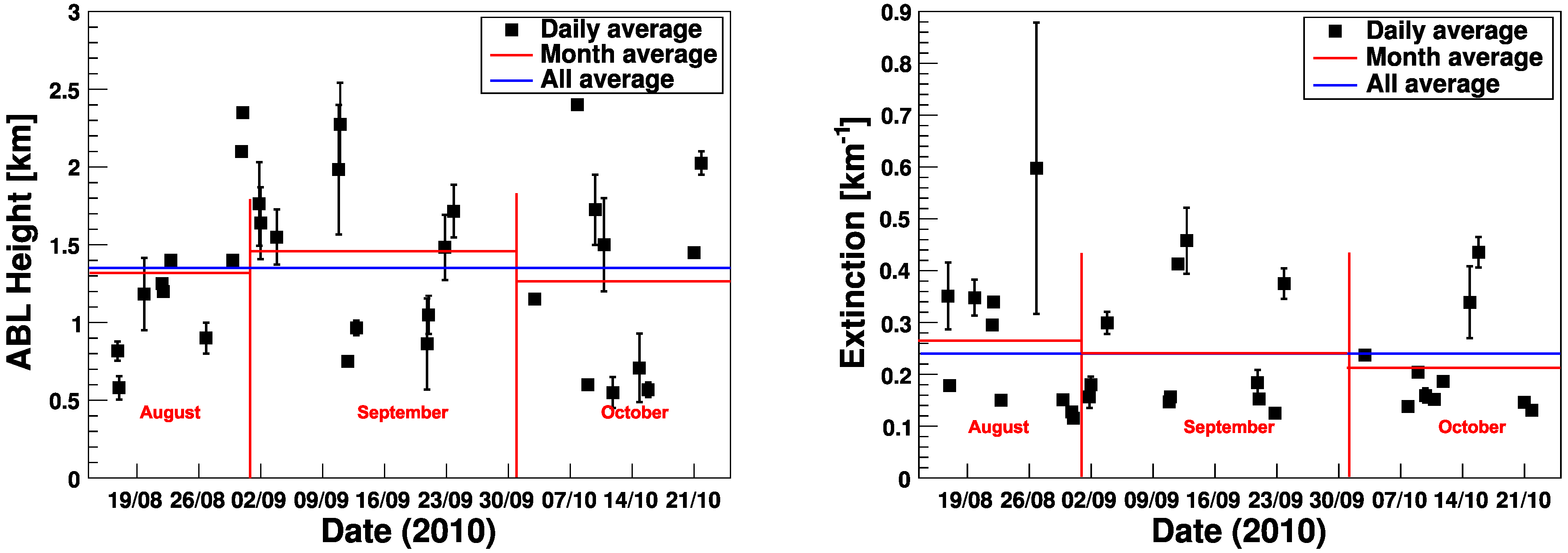
In most cases, AOD along the height was retrieved up to the height of 3 km, and aerosol extinction was retrieved up to 2.5 km above the LiDAR site, which was typically above the ABL height in Europe. Within this height, several aerosol layers were found constantly in almost all cases, showing atmospheric characteristic fluctuations caused by the individual turbulence elements. The ABL height can be easily determined from the aerosol extinction profile, where a sharp decrease happened or a minimum value was found. The daily average ABL heights from those measurements are shown in
Figure 7 (left). The error bar denotes the measurement uncertainties for the section. As different numbers of measurements were performed in each section, data points without an error bar were the results with only one performed measurement. The average ABL height between August and October 2010 was about 1.35 km above the LiDAR site. However, the average ABL height in September 2010 was a bit higher than that in August and October 2010. The average aerosol extinction within the ABL on the basis of measurements from 16 August to 21 October 2010 is shown in
Figure 7. More than half of the values of the average aerosol extinction were below 0.3 km
−1, showing that the atmosphere in this region contained little aerosol loading. One exception is the data on 26 August, which had an average aerosol extinction larger than 0.6 km and an average ABL height lower than 1.0 km. However, large uncertainty of aerosol extinction and small uncertainty of ABL height were obtained, as well, which could be explained as a result of turbulent changing of aerosol loading, mostly from the ground within the ABL during the measuring section. The average value of aerosol extinction from August to October 2010 decreased linearly, which could be the result of the influence of local sources or large-scale flows. The average value of aerosol extinction during these three months was about 0.24 km
−1.
To explain the variability of aerosol loading in the study region, especially within the ABL, air flow trajectories at three different heights (1.0 km, 1.5 km and 2.0 km) were modeled using HYSPLIT [
32] for all the dates when measurements were performed. In a few hours, air flow directions of backward trajectories changed very little. Therefore, 48-hour backward trajectories were selected with an end time of 21:00 UTC for the first half of the night and with the an end time of 01:00 UTC for the second half of the night.
Figure 7.
Atmospheric boundary layer (ABL) heights derived from the 2D RHI scanning measurements between 16 August and 21 October 2010. Also shown is the average height of the ABL in each month and in all three months. Height is given relative to the altitude of the LiDAR site.
Figure 7.
Atmospheric boundary layer (ABL) heights derived from the 2D RHI scanning measurements between 16 August and 21 October 2010. Also shown is the average height of the ABL in each month and in all three months. Height is given relative to the altitude of the LiDAR site.
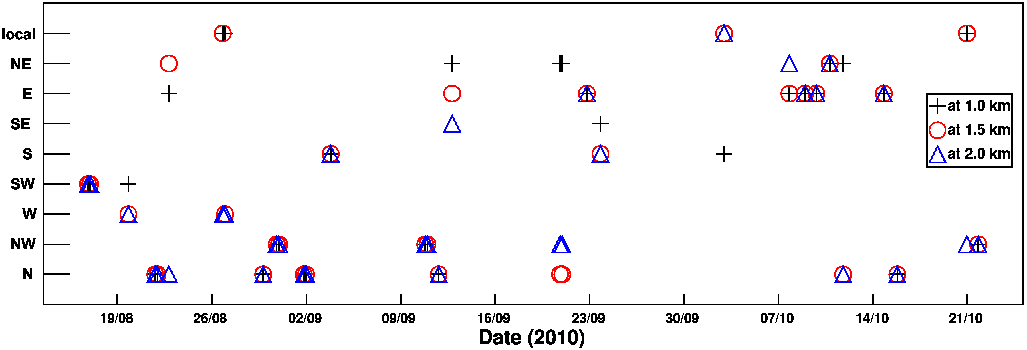
Nine classes have been defined representing the origin of air mass, namely north (N), northwest (NW), west (W), southwest (SW), south (S), southeast (SE), east (E), northeast (NE) and “local”. The class “local” represents very short trajectories with an air parcel staying for a long time close to the study region. The statistical distribution of trajectory classes on the days when LiDAR measurements were performed is shown in
Figure 8. In most cases, air flows at all three investigated heights had the same directions. Seventy two percent of backward trajectories were from the northwest, north, northeast and east, which carried aerosols from the mainland of Europe; 14% of backward trajectories were from the southwest and south, showing that the atmospheric conditions in the study region were influenced by marine aerosols from the Mediterranean or Adriatic Sea. LiDAR results of aerosol extinction showed that aerosol loading could change totally from day to day, which was in agreement with the variation of the history of air masses transported to this region.
Figure 8.
Origin of the air mass estimated from the backward trajectories using the Hybrid Single Particle Lagrangian Integrated Trajectory Model. Three different heights in the lower troposphere (1.0 km, 1.5 km and 2.0 km) were checked.
Figure 8.
Origin of the air mass estimated from the backward trajectories using the Hybrid Single Particle Lagrangian Integrated Trajectory Model. Three different heights in the lower troposphere (1.0 km, 1.5 km and 2.0 km) were checked.
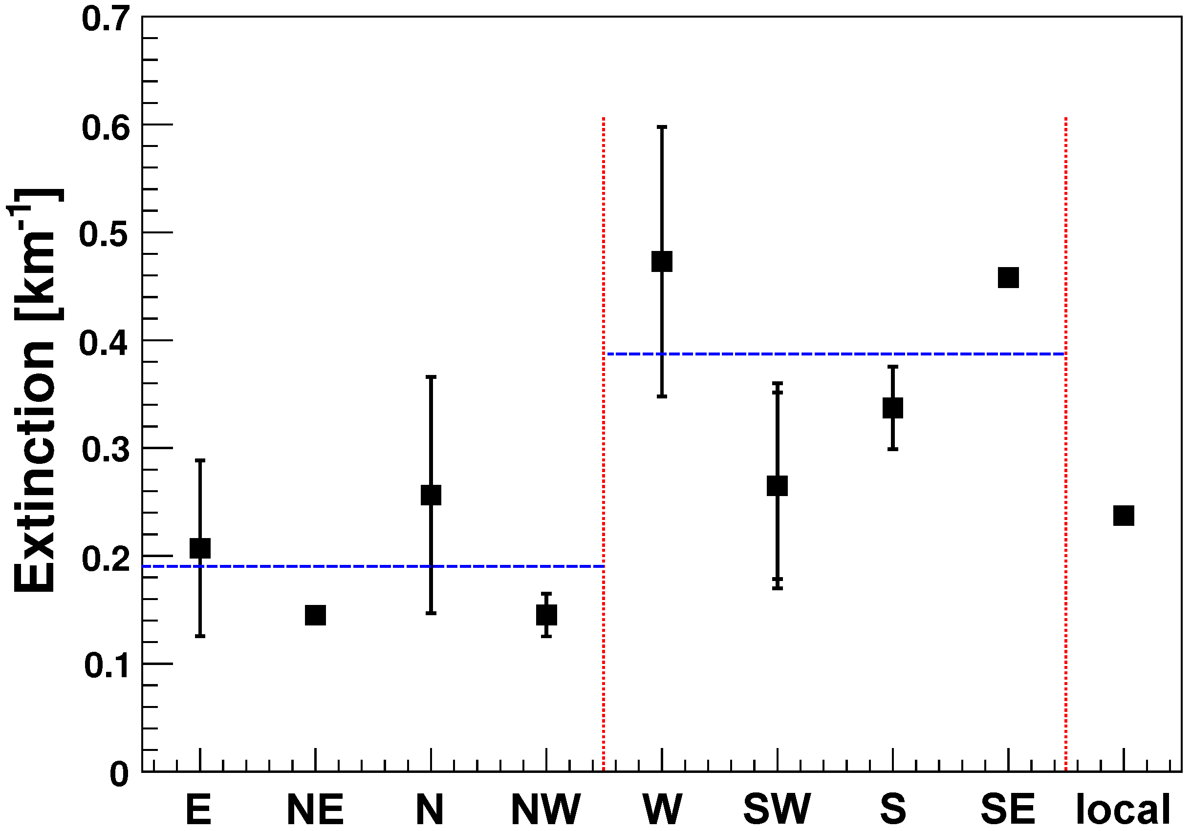
Considering that air flow directions at the heights of 1.0 km, 1.5 km and 2.0 km were almost the same, we used the air mass class from the height of 2 km for the analysis of aerosol extinction. The mean aerosol extinction within the ABL for each of the nine classes is shown in
Figure 9. Two groups of classes with different characteristics were found: one includes the E, NE, N and NW classes, which exhibited small average aerosol extinction values (< 0.26 km
−1); the other group comprises the W, SW, S and SE classes with large average aerosol extinction values (> 0.27 km
−1). The average value of aerosol extinction in the first group was around 0.2 km
−1, which agreed with the presence of land-based air masses from the European continent. The average value of aerosol extinction in the second group was two-times larger (0.4 km
−1), which could be the result of the influence of marine aerosols from the Mediterranean or Adriatic Sea.
Figure 9.
Mean aerosol extinction within the ABL depending on the origin of the air mass. Error bars represent the standard deviation of the measurement results.
Figure 9.
Mean aerosol extinction within the ABL depending on the origin of the air mass. Error bars represent the standard deviation of the measurement results.
6. Conclusions
Aerosol variability over the southwest region of Slovenia was investigated by using an ultraviolet scanning elastic backscatter LiDAR. The vertical scans were performed over the Vipava Valley, the Karst Plateau and the Bay of Trieste. With the assumption of horizontal atmospheric homogeneity, aerosol optical variables were retrieved by using the multiangle retrieval method.
In data processing, construction of the Cartesian 2D RHI diagram was done using barycentric interpolation of the weighted logarithm RSCS values. Correction of Rayleigh scattering was implemented to eliminate the influence of molecular elastic scattering of ultraviolet light on the retrieval of aerosol optical variables. The feasibility of the assumption of horizontal atmospheric homogeneity in the study region was assessed by extracting the horizontal pixel data points from the 2D RHI diagram and investigating the linearity of the constructed line with the distance from the LiDAR site. The performed measurement on 12 October 2011 showed the capability of the ultraviolet scanning LiDAR for probing the aerosol extinction and determination of the ABL height.
The statistics of three months’ observations from August to October 2010 was implemented to investigate aerosol variability, combined with the modeling of air flow trajectories using HYSPLIT for the dates when measurements were performed. LiDAR results of aerosol extinction showed that aerosol loading was in agreement with the variation of the history of air masses transported to this region. The aerosol from the Mediterranean or Adriatic Sea gave a bigger influence than that with the presence of land-based air masses from the European continent.


 ,
, 


