Seasonal Variations of the Relative Optical Air Mass Function for Background Aerosol and Thin Cirrus Clouds at Arctic and Antarctic Sites

Abstract

New calculations of the relative optical air mass function are made over the 0°–87° range of apparent solar zenith angle θ, for various vertical profiles of background aerosol, diamond dust and thin cirrus cloud particle extinction coefficient in the Arctic and Antarctic atmospheres. The calculations were carried out by following the Tomasi and Petkov (2014) procedure, in which the above-mentioned vertical profiles derived from lidar observations were used as weighting functions. Different sets of lidar measurements were examined, recorded using: (i) the Koldewey-Aerosol-Raman Lidar (KARL) system (AWI, Germany) at Ny-Ålesund (Spitsbergen, Svalbard) in January, April, July and October 2013; (ii) the Cloud-Aerosol Lidar and Infrared Pathfinder Satellite Observations (CALIPSO) satellite-based sensor over Barrow (Alaska), Eureka (Nunavut, Canada) and Sodankylä (northern Finland), and Neumayer III, Mario Zucchelli and Mirny coastal stations in Antarctica in the local summer months of the last two years; (iii) the National Institute of Optics (INO), National Council of Research (CNR) Antarctic lidar at Dome C on the Antarctic Plateau for a typical “diamond dust” case; and (iv) the KARL lidar at Ny-Ålesund and the University of Rome/National Agency for New Technologies, Energy and Sustainable Economic Development (ENEA) lidar at Thule (northwestern Greenland) for some cirrus cloud layers in the middle and upper troposphere. The relative optical air mass calculations are compared with those obtained by Tomasi and Petkov (2014) to define the seasonal changes produced by aerosol particles, diamond dust and cirrus clouds. The results indicate that the corresponding air mass functions generally decrease as angle θ increases with rates that are proportional to the increase in the pure aerosol, diamond dust and cirrus cloud particle optical thickness.

1. Introduction

Regular sun-photometer measurements are currently conducted at numerous Arctic and Antarctic sites to determine the spectral values of aerosol optical thickness τ_a(λ) at visible and near-infrared wavelengths [1]. These measurements are conducted using different sun-photometer models such as the Cimel CE-318 of the Aerosol Robotic Network (AERONET) network [2], the Prede POM-01L and POM-02L sun/sky-radiometers of the SKYNET network [3], the hand-held Microtops sun-photometers of the Maritime Aerosol Network (MAN) [4], the EKO MS-110 model [5] used by the Japan Meteorological Agency (Tokyo, Japan) at Syowa (Antarctica), and various sun-photometer models employed by the POLAR-AOD partners [6,7]. An extensive list of the multispectral sun-photometers employed at numerous Arctic and Antarctic sites to carry out the routine activities planned by various networks to measure the aerosol optical depth τ_a(λ) during the past two decades is given in Table 1, providing also the peak-wavelengths of the narrow-band interference filters mounted on the sun-photometers, and the references where the technical characteristics of these instruments are available.

Following the criteria established by the multispectral sun-photometry method [18], each measurement of direct solar irradiance J(λ) (performed at a window-wavelength λ for a certain apparent solar zenith angle θ on a cloudless day) is examined in terms of the Lambert-Beer law to determine the total optical thickness τ(λ) of the atmosphere in terms of the following analytical form obtained by inverting the well-known Lambert-Beer law:

$$\tau (\lambda )=(1/m)\ln \left[D{J}_o(\lambda )/J(\lambda )\right]$$

(1)

where: m is the relative optical air mass of the atmosphere for angle θ, D is the factor taking into account the day-to-day variations in the direct solar irradiance due to the changes in the Earth-Sun distance throughout the year [19], and J_o(λ) is the output voltage that would be measured by the sun-photometer outside the atmosphere. The spectral values of J_o(λ) are usually determined by applying the Langley plot method to measurements carried out at high-altitude sites on days characterized by stable atmospheric turbidity conditions [20]. Equation (1) shows that the instantaneous values of m need to be accurately known in order to determine the monochromatic value of τ(λ) with the best precision. This is particularly important in the polar regions, where the aerosol optical thickness τ_a(λ) is often very low [6], and aerosol radiative effects may be not negligible [21]. A set of appropriate values of m was calculated by Tomasi and Petkov [22] (hereinafter referred to as TP2014) at Arctic and Antarctic sites over the 0° ≤ θ ≤ 87° range. The dependence of air refractive index on the vertical profiles of pressure p(z), temperature T(z) and water vapor partial pressure e(z) in the polar atmospheres was taken into account by using the algorithm of Tomasi et al. [23] applied to the average vertical profiles of p(z), T(z) and e(z) derived from the radiosounding data collected at Ny-Ålesund (~79°N) in Spitsbergen (Svalbard) during June and July in the years from 2000–2003 [24], and from those recorded at Mario Zucchelli (~75°S) during the austral summer season from 1987 to 1998 [25].

Table 1. List of the multispectral sun-photometer models employed at the Arctic and Antarctic stations of the various networks, with the sun-photometric channel peak-wavelengths at which aerosol optical depth τ_a(λ) is routinely measured. The last column provides the main references where the technical characteristics of the various instruments are available.

Ablesun-Photometer Model	Arctic Stations	Antarctic Stations	Peak-Wavelengths (nm)	References
Cimel CE-318 sun-photometer model of the AERONET and AEROCAN networks	Barrow (Alaska, USA); Resolute Bay (Nunavut, Canada); Eureka 0PAL (Nunavut, Canada); Eureka PEARL (Nunavut, Canada); Thule (North-Western Greenland); Ittoqqortoormiit (Eastern Greenland); Hornsund (Spitsbergen, Svalbard); Andenes (Norway); Sodankylä (Finland); Tiksi (NE Siberia, Russia)	Marambio (Argentina); Vechernaya Hill (Belarus); Utsteinen Ridge (Belgium); McMurdo (USA); Dome C (France/Italy); South Pole (USA)	340, 380, 440, 500, 675, 870, 1020	Holben et al. [2]
Precision Filter Radiometer PFR of the GAW-PFR Network, PMOD/WRC (Davos, Switzerland)	Summit (Central Greenland); Ny-Ålesund (Spitsbergen, Svalbard); Kiruna (Sweden); Sodankylä (Finland)	Troll (Norway)	367.6, 367.7, 368.0, 368.7, 368.9, 411.4, 411.9, 412.0, 412.1, 499.7, 500.0, 500.5, 500.6, 861.6, 862.0, 862.2, 862.5	Wehrli [8]
Carter Scott SP01, SP01-A, SP02 and SP022 models of the GMD/NOAA (Boulder, Colorado, USA)	Barrow (Alaska, USA); Alert (Nunavut, (Canada)	Dome C (France/Italy); South Pole (USA)	367, 368, 412, 413, 500, 610, 675, 778, 862, 865, 1050	Stone [9]
Prede POM-01L and POM-02L models of the NIPR (Tokyo, Japan); Prede POM-02L model of the ISAC-CNR Institute (Rome, Italy), and Prede POM-01L model of the British Antarctic Survey (BAS) (Cambridge, UK) of the SKYNET network	Ny-Ålesund (Spitsbergen, Svalbard)	Syowa (Japan); Rothera (UK); Halley (UK); Mario Zucchelli (Italy)	315, 340, 380, 400, 500, 675, 870, 1020, 1627, 2200	Shiobara et al. [10], di Carmine et al. [11]
SP1A and SP2H sun-photometer models and STAR 01 star-photometer of the Alfred Wegener Institute (AWI, Bremenhaven, Germany)	Ny-Ålesund (Spitsbergen, Svalbard)	Neumayer (Germany)	351, 367, 371, 380, 390, 413, 416, 441, 443, 500, 501, 531, 532, 605, 609, 673, 675, 776, 778, 862, 864, 1023, 1025, 1045, 1046, 1062	Herber et al. [12]
ABAS sun-photometer of the Alfred Wegener Institute (AWI, Bremenhaven, Germany) and the Arctic and Antarctic Research Institute (AARI, St. Petersburg, Russia)	-	Neumayer (Germany); Mirny (Russia)	395, 408, 479, 581, 651, 789, 873, 1041	Leiterer and Weller [13], Radionov et al. [14]
Portable SPM models of the Institute of Atmospheric Optics (IAO), Siberian Branch (SB), Russian Academy of Sciences (RAS) (Tomsk, Russia)	Barentsburg (Spitsbergen, Svalbard)	Mirny (Russia)	339, 340, 379, 380, 442, 443, 499, 500, 547, 548, 675, 676, 871, 1019, 1020, 1240, 1244, 1553, 1555, 2134	Sakerin et al. [15]
Handheld Microtops II of the Space Physics Laboratory, Trivandrum (India), the IAO-SB-RAS (Tomsk, Russia), the AARI Institute (St. Petersburg, Russia), and the OPAR Institute, University of Réunion, Saint Denis de la Réunion (France)	Ny-Ålesund (Spitsbergen, Svalbard)	Mirny (Russia); Novolazarevskaya (Russia); Dome C (France/Italy)	379, 440, 441, 500, 674, 675, 868, 870	Smirnov et al. [4]
EKO MS-110 of the Japan Meteorological Agency (JMA) (Tokyo, Japan)	--	Syowa (Japan)	368, 500, 675, 778, 862	Ohno [5]
UVISIR-2, FISBAT and ASP-15WL sun-photometer models of the ISAC-CNR Institute (Bologna, Italy)	--	Mario Zucchelli (Italy)	320.2, 321.0, 335.3, 342.0, 359.8, 370.0, 381.0, 400.2, 401.3, 411.5, 441.5, 450.5, 459.6, 499.5, 500.6, 505.9, 550.0, 551.0, 610.0, 669.7, 671.3, 672.5, 774.6, 780.0, 861.2, 865.2, 868.0, 1025.7, 1040.6, 1047.4	Tomasi et al. [6,16,17]

Table 1. List of the multispectral sun-photometer models employed at the Arctic and Antarctic stations of the various networks, with the sun-photometric channel peak-wavelengths at which aerosol optical depth τ_a(λ) is routinely measured. The last column provides the main references where the technical characteristics of the various instruments are available.

Ablesun-Photometer Model	Arctic Stations	Antarctic Stations	Peak-Wavelengths (nm)	References
Cimel CE-318 sun-photometer model of the AERONET and AEROCAN networks	Barrow (Alaska, USA); Resolute Bay (Nunavut, Canada); Eureka 0PAL (Nunavut, Canada); Eureka PEARL (Nunavut, Canada); Thule (North-Western Greenland); Ittoqqortoormiit (Eastern Greenland); Hornsund (Spitsbergen, Svalbard); Andenes (Norway); Sodankylä (Finland); Tiksi (NE Siberia, Russia)	Marambio (Argentina); Vechernaya Hill (Belarus); Utsteinen Ridge (Belgium); McMurdo (USA); Dome C (France/Italy); South Pole (USA)	340, 380, 440, 500, 675, 870, 1020	Holben et al. [2]
Precision Filter Radiometer PFR of the GAW-PFR Network, PMOD/WRC (Davos, Switzerland)	Summit (Central Greenland); Ny-Ålesund (Spitsbergen, Svalbard); Kiruna (Sweden); Sodankylä (Finland)	Troll (Norway)	367.6, 367.7, 368.0, 368.7, 368.9, 411.4, 411.9, 412.0, 412.1, 499.7, 500.0, 500.5, 500.6, 861.6, 862.0, 862.2, 862.5	Wehrli [8]
Carter Scott SP01, SP01-A, SP02 and SP022 models of the GMD/NOAA (Boulder, Colorado, USA)	Barrow (Alaska, USA); Alert (Nunavut, (Canada)	Dome C (France/Italy); South Pole (USA)	367, 368, 412, 413, 500, 610, 675, 778, 862, 865, 1050	Stone [9]
Prede POM-01L and POM-02L models of the NIPR (Tokyo, Japan); Prede POM-02L model of the ISAC-CNR Institute (Rome, Italy), and Prede POM-01L model of the British Antarctic Survey (BAS) (Cambridge, UK) of the SKYNET network	Ny-Ålesund (Spitsbergen, Svalbard)	Syowa (Japan); Rothera (UK); Halley (UK); Mario Zucchelli (Italy)	315, 340, 380, 400, 500, 675, 870, 1020, 1627, 2200	Shiobara et al. [10], di Carmine et al. [11]
SP1A and SP2H sun-photometer models and STAR 01 star-photometer of the Alfred Wegener Institute (AWI, Bremenhaven, Germany)	Ny-Ålesund (Spitsbergen, Svalbard)	Neumayer (Germany)	351, 367, 371, 380, 390, 413, 416, 441, 443, 500, 501, 531, 532, 605, 609, 673, 675, 776, 778, 862, 864, 1023, 1025, 1045, 1046, 1062	Herber et al. [12]
ABAS sun-photometer of the Alfred Wegener Institute (AWI, Bremenhaven, Germany) and the Arctic and Antarctic Research Institute (AARI, St. Petersburg, Russia)	-	Neumayer (Germany); Mirny (Russia)	395, 408, 479, 581, 651, 789, 873, 1041	Leiterer and Weller [13], Radionov et al. [14]
Portable SPM models of the Institute of Atmospheric Optics (IAO), Siberian Branch (SB), Russian Academy of Sciences (RAS) (Tomsk, Russia)	Barentsburg (Spitsbergen, Svalbard)	Mirny (Russia)	339, 340, 379, 380, 442, 443, 499, 500, 547, 548, 675, 676, 871, 1019, 1020, 1240, 1244, 1553, 1555, 2134	Sakerin et al. [15]
Handheld Microtops II of the Space Physics Laboratory, Trivandrum (India), the IAO-SB-RAS (Tomsk, Russia), the AARI Institute (St. Petersburg, Russia), and the OPAR Institute, University of Réunion, Saint Denis de la Réunion (France)	Ny-Ålesund (Spitsbergen, Svalbard)	Mirny (Russia); Novolazarevskaya (Russia); Dome C (France/Italy)	379, 440, 441, 500, 674, 675, 868, 870	Smirnov et al. [4]
EKO MS-110 of the Japan Meteorological Agency (JMA) (Tokyo, Japan)	--	Syowa (Japan)	368, 500, 675, 778, 862	Ohno [5]
UVISIR-2, FISBAT and ASP-15WL sun-photometer models of the ISAC-CNR Institute (Bologna, Italy)	--	Mario Zucchelli (Italy)	320.2, 321.0, 335.3, 342.0, 359.8, 370.0, 381.0, 400.2, 401.3, 411.5, 441.5, 450.5, 459.6, 499.5, 500.6, 505.9, 550.0, 551.0, 610.0, 669.7, 671.3, 672.5, 774.6, 780.0, 861.2, 865.2, 868.0, 1025.7, 1040.6, 1047.4	Tomasi et al. [6,16,17]

As pointed out by TP2014 [22], the product m τ(λ) is equal to the sum of the following contributions: (i) the product of the atmospheric relative optical air mass m by the Rayleigh scattering optical thickness τ_R(λ), (ii) the product of the relative optical air mass m_a for aerosol extinction by the aerosol optical thickness τ_a(λ), and (iii) the sum of the products of relative optical air mass m_j for the j-th atmospheric gaseous constituent by the corresponding optical thickness τ_j(λ), where j identifies each gaseous constituent causing weak absorption within the sun-photometer spectral channels.

Therefore, τ_a(λ) can be calculated as

$${\tau }_a(\lambda )=(1/m_a)\left[m\tau (\lambda )-m{\tau }_R(\lambda )-{\displaystyle {\sum }_j{m}_j{\tau }_j}(\lambda )\right]$$

(2)

where the subscript j refers to atmospheric water vapor, ozone, nitrogen dioxide (together with its dimer N₂O₄), and oxygen dimer (O₄). Simulations of the atmospheric absorption spectrum of incoming solar radiation made over the 0.30–1.10 µm wavelength range by using the MODTRAN 2/3 code and the LOWTRAN 7 model [26] for the Subarctic Summer atmospheric model [27] indicate that: (i) numerous absorption bands of water vapor are centered at the 591, 650, 695, 702, 720, 730, 820, 906, 936, 950 and 975 nm wavelengths, with intensities gradually increasing with wavelength; (ii) the strong wing of the ozone Huggins band is present from 0.30 to 0.35 µm and the wide Chappuis band covers the 407–750 nm wavelength range, presenting semi-continuous absorption features having the maximum at the 602 nm wavelength; (iii) the semi-continuum of nitrogen dioxide NO₂, superimposed with the absorption effects of its dimer N₂O₄, exhibits a spectral absorption curve gradually decreasing from 400 to 660 nm; and (iv) the oxygen dimer (O₄) displays a sequence of six absorption bands from 430 to 1140 nm, centered at the 446, 476, 532, 577, 628 and 1065 nm wavelengths [28].

In order to calculate τ_a(λ) with a good accuracy, we recommend to use in Equation (2): (i) the values of m for Rayleigh scattering determined separately for the Arctic and Antarctic atmosphere [22], and (ii) the values of m_j defined for the four minor absorbing gases separately for the Arctic atmosphere (at Ny-Ålesund, ~79°N latitude) and the Antarctic atmosphere (Mario Zucchelli, ~75°S latitude).

The relative optical air mass m_a for aerosols was derived for 0° ≤ θ ≤ 87° [22] and the following vertical profiles of aerosol extinction coefficient: (i) background Arctic aerosol observed in summer; (ii) average haze observed at Ny-Ålesund in winter−spring 2002; (iii) dense Arctic haze observed at Ny-Ålesund on 2 May 2006; (iv) Kasatochi volcanic particles observed at Ny-Ålesund in late August and early September of 2008 [29]; (v) background Antarctic aerosol measured at coastal sites during the austral summer; and (vi) aged volcanic particles measured by a lidar located at McMurdo on 1 June 1993, two years after the Pinatubo eruption.

These calculations describe the mean behavior of m_a for different atmospheric turbidity conditions in the Arctic and Antarctic atmospheres. Therefore, seasonal changes of m_a(θ) or its dependence on the measurement site are not discussed by TP2014 [22]. Moreover, no information was given on the behavior of m_a(θ) in cases of upper tropospheric thin cirrus cloud layers or marked diamond dust loads close to the surface. These aspects are examined in the present study.

In particular, the main purpose of the present calculations is to (1) ascertain the variability of m_a(θ) for different vertical profiles of the aerosol volume extinction coefficient k_a(z) at various Arctic and Antarctic sites and (2) estimate the values of m_a(θ) to be used when particulate matter layers are suspended at various tropospheric altitudes (such as a diamond dust close to the ground or a thin cirrus cloud layer in the mid- or upper troposphere). The values of m_a(θ) obtained in the different cases are compared with the calculations made by TP2014 [22], which provide reference cases for background summer aerosol loads in the two polar atmospheres. The new calculations of m_a(θ) given in the present study and those provided by TP2014 [22] may be usefully employed to determine more accurately the atmospheric turbidity parameters given by polar aerosols and improve the analysis of the ground-based sun-photometer data collected during the new field campaigns conducted by the AERONET, AEROMAN, AEROCAN, GAW-PFR, SKYNET and Japan Meteorological Agency (JMA) networks mentioned in Table 1. The present results may be also used in order to implement more accurate radiative transfer calculations in the polar atmospheres for thin cirrus clouds or diamond dust layers at tropospheric layers.

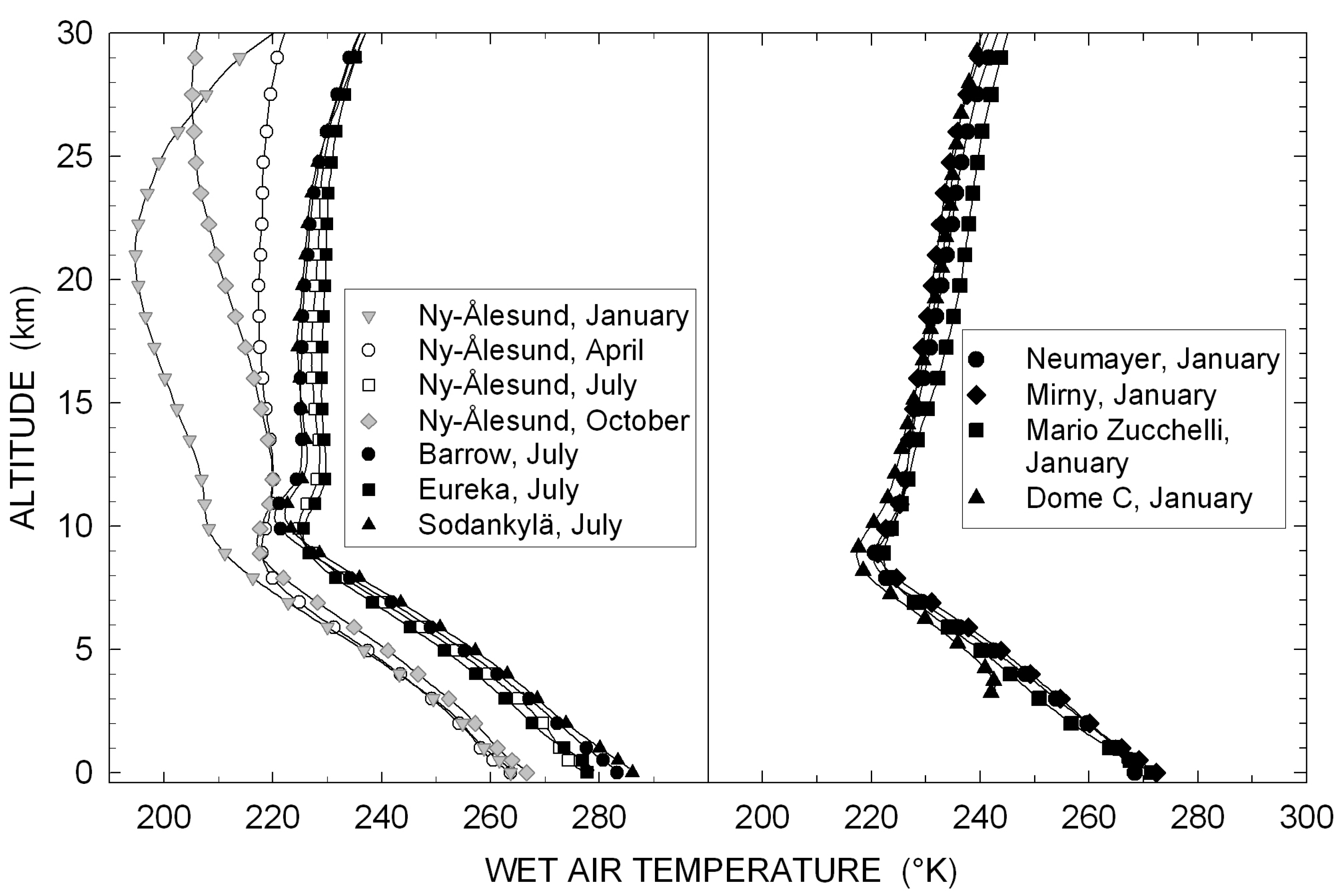
2. The Atmospheric Model used to Calculate the Relative Optical Air Mass Functions and Determination of the Vertical Profiles of Aerosol Volume Extinction Coefficient

The present calculations of m_a(θ) were made following the TP2014 [22] procedure based on the general scheme of the Earth-atmosphere system proposed by Thomason et al. [30]. The calculations apply to an incoming direct solar radiation beam propagating through a spherical atmosphere. The wet-air refraction effects closely related to the pressure and temperature variations with height, and the Earth’s curvature are taken into account. In the specific cases of aerosol or cloud particle extinction, the relative optical air mass m_a(θ) has been calculated over the 0° ≤ θ ≤ 87° range by using the following formula:

$$m_a(\theta )=\frac{1}{K_a}{\displaystyle {\int }_{z_o}^{z_{\infty }}\frac{k_a(z)dz}{\sqrt{1-\frac{n_o}{n(z)}{(z_o/z)}^2{\sin }^2\theta }}}$$

(3)

where: (i) k_a(z) is the vertical profile of the volume extinction coefficient produced by aerosols or cloud particles, calculated in km⁻¹ over the altitude range from the mean sea-level z_o to the atmospheric top-level z_∞ (assumed to be of 120 km in all cases); (ii) K_a is the integral of k_a(z) made over the z_o ≤ z ≤ z_∞ altitude range, which in practice equal to the aerosol optical thickness τ_a(λ) measured at a certain wavelength λ; (iii) n_o is the air refractive index at sea-level z_o; and (iv) n(z) is the air refractive index varying as a function of z. It can be clearly seen in Equation (3) that k_a(z) is used as a weighting function to evaluate the solar radiation extinction effects versus altitude.

TP2014 [22] used vertical profiles of p(z), T(z) and e(z) derived from radiosoundings to better characterize the dependence of n(z) on altitude. The radiosounding datasets were based on measurements made at Ny-Ålesund (~79°N) during June-July of 2000–2003 [24], and at Mario Zucchelli (~75°S) during the austral summer season from 1987 to 1998 [25]. Above 30 km altitude, the profiles were completed with (i) monthly mean vertical profiles of the three thermodynamic parameters obtained by Tomasi et al. [31] from multi-year Michaelson Interferometer for Passive Atmospheric Sounding (MIPAS)-Environmental Satellite (ENVISAT) limb-scanning measurements over the 33–60 km altitude range at 80°N in July and at 75°S in January, and (ii) the vertical profiles p(z) and T(z) defined in the AFGL Subarctic Summer model over the 70–120 km altitude range [27]. The combined average vertical profiles of p(z), T(z) and e(z) were used in the Tomasi et al. [23] algorithm to calculate the vertical profiles of n(z) in the Arctic and Antarctic atmospheres. The values of n_o were determined for the ground-level measurements of the air thermodynamic parameters.

In the present study, m_a(θ) was calculated using Equation (3) with the values of n(z) and n_o derived from the following radiosounding datasets and meteorological data recorded at the following sites:

(i) at Ny-Ålesund (78°54'N, 11°53'E, 5 m a.m.s.l. (above mean sea level)) on the Kongsfjorden (Spitsbergen, Svalbard), the radiosounding profiles measured in January, April, July and October of the 5-year period from 2005 to 2009, and analysed using the Tomasi et al. [24] procedure;

(ii) at Barrow (71°19'N, 156°36'W, 8 m a.m.s.l.) in northern Alaska (USA) on the Arctic Ocean coast, the radiosounding data collected in July from 2005 to 2009;

(iii) at Eureka (79°59'N, 85°56'W, 11 m a.m.s.l.), located on the Fosheim Peninsula (Ellesmere Island, Qikiqtaaluk, Nunavut, Canada), the radiosounding data taken in July from 2000 to 2003 [24];

(iv) at Sodankylä (67°22'N, 26°38'E, 184 m a.m.s.l.) in northern Finland, the radiosounding data collected in July from 2005 to 2009;

(v) at Neumayer III (70°39'S, 08°15'W, 40 m a.m.s.l.), on the Ekström Shelf Ice near the Atka Bay in the northeastern part of Weddell Sea, the radiosounding profiles made by the Alfred Wegener Institute (AWI, Bremerhaven, Germany) group in January from 2000 to 2003 [24];

(vi) at Mirny (66°33'S, 93°01'E, 40 m a.m.s.l.), on the Antarctic coast of the Davis Sea in the Australian Antarctic Territory, the radiosounding data collected by AARI (Russia) in July from 1998 to 2010;

(vii) at Mario Zucchelli (74°42'S, 164°07'E, 15 m a.m.s.l.), on the Terra Nova Bay coast (Ross Sea, Victoria Land), the Vaisala radiosonde data collected by the Meteo-Climatological Observatory of the Italian Antarctic Project (ENEA, C. R. Casaccia, Rome, Italy) (http://www.climantartide.it) in January from 1987 to 1998 [25]; and

(viii) at Dome Concordia (also named Dome C) (75°06'S, 123°21'E, 3233 m a.m.s.l.) on the Eastern Antarctic Plateau, for the Vaisala radiosounding data collected by the Meteo-Climatological Observatory of the Italian Antarctic Project (ENEA, C. R. Casaccia, Rome, Italy) over the 4-year period from March 2005 to March 2009 [31].

The analysis of the various datasets produced monthly mean vertical profiles of p(z), T(z) and e(z), which were used to determine the average vertical profiles of n(z) at the various polar sites for the different months. As shown by Tomasi et al. [24], the monthly mean vertical profiles of pressure p(z) regularly decrease in an exponential fashion as a function of altitude over the whole range, while relative humidity decreases in general with height until reaching values of a few percent at the tropopause level and low stratosphere altitudes [25]. The rather low values of e(z) correspondingly found usually in both polar atmospheres for cloudless conditions exert a weak influence on n(z). Conversely, appreciable variations in the monthly mean temperature profiles are observed during the local summer months at all the Arctic and Antarctic sites, in agreement with the results by Tomasi et al. [24]. The monthly mean vertical profiles of T(z) obtained from the radiosounding datasets at the eight polar sites are presented in Figure 1, showing that T(z) gradually decreases with altitude until reaching a minimum at the tropopause level found between 8 and 10 km. The temperatures measured in April and October at Ny-Ålesund are appreciably lower (by more than 10 K) than those measured in July at Ny-Ålesund and the other Arctic sites. The values measured in January are close to those of October at all the tropospheric levels, and are considerably lower than in October at all stratospheric levels z > 8 km. The summer profiles of T(z) measured at the four Arctic sites differ by less than 10 K, and display similar vertical gradients. The changes are larger in the lower stratosphere than in the troposphere. In Antarctica, the January (austral summer) profiles of T(z) are similar at all four sites, both in the troposphere and in the lower stratosphere. The temperature profiles at Dome C, which is a high altitude sites, is characterized by a significant thermal inversion in the lowest atmospheric layers, differently from the other sites.

Figure 1. Monthly mean vertical profiles of wet air temperature T(z) derived over the 0 ≤ z ≤ 30 km altitude range from the multi-year radiosounding datasets collected at Ny-Ålesund in four different months and at three other Arctic sites in July (left-hand side), and at four Antarctic sites in January (right-hand side). Note that the vertical profile of T(z) (solid triangles) measured at Dome C on the Antarctic Plateau starts at the (surface-level) altitude of 3.233 km.

Figure 1. Monthly mean vertical profiles of wet air temperature T(z) derived over the 0 ≤ z ≤ 30 km altitude range from the multi-year radiosounding datasets collected at Ny-Ålesund in four different months and at three other Arctic sites in July (left-hand side), and at four Antarctic sites in January (right-hand side). Note that the vertical profile of T(z) (solid triangles) measured at Dome C on the Antarctic Plateau starts at the (surface-level) altitude of 3.233 km.

The values of k_a(z) and its integral K_a used in Equation (3) were calculated by TP2014 [22] for various particle extinction profiles. Coefficient k_a(z) was obtained from lidar measurements of the volume backscattering coefficient B_bs(0.532 μm) multiplied by the value of lidar ratio for tropospheric aerosols derived from inelastic scattered lidar returns of N₂ molecules, according to Ansmann et al. [32]. The integral of K_a(z) was calculated and compared with the measured value of τ_a(0.532 μm), as made by Hoffmann et al. [29]. A value of lidar ratio equal to 40 sr at the 0.532 μm wavelength was used in the present study: A possible error in estimating the lidar ratio should cause an uncertainty in K_a(z) not exceeding 10%.

Vertical profiles of k_a(z) were selected at various Arctic and Antarctic sites to represent the average extinction of background aerosols in the troposphere and low stratosphere during the local summer months. The background aerosol cases do not include volcanic particles in the lower stratosphere, nor Arctic haze, biomass burning smoke or Asian dust layers in the lower troposphere. More precisely, the following aerosol and cloud particle extinction profiles were considered in the present study:

(1) The mean profile of k_a(z) derived from monthly or multi-monthly average B_bs(0.532 μm) profiles measured at Ny-Ålesund with the AWI (Alfred Wegener Institute, Germany) KARL (Koldewey-Aerosol-Raman Lidar) lidar-system (described by Hoffmann et al. [33]) in January, April, June−July and October−December of 2013 (see also [1]).

(2) Multi-month average vertical profiles of k_a(z) derived from observations by the CALIOP (Cloud-Aerosol Lidar with Orthogonal Polarization) lidar onboard the CALIPSO (Cloud-Aerosol Lidar and Infrared Pathfinder Satellite Observations) satellite. Profiles over 2° latitude × 5° longitude sectors centerd at Barrow, Eureka and Sodankylä were selected. The Level-3 satellite data for the summer (June−September) months of the last two years were taken from the https://eosweb.larc.nasa.gov/project/calipso/cal_lid_l3_apro_combined-beta-v1-30_table and http://reverb.echo.nasa.gov/reverb websites, as a part of the “Cloud-Free + Above (Combined) Aerosol Extinction Profiles”, Version 1.30, Beta (codex CAL_LID_L3_APro_Combined-Beta-V1-30) dataset. It is worth mentioning that for cloud-free conditions in the planetary boundary layer the vertical profiles of aerosol extinction coefficient derived from CALIOP measurements were evaluated by Kim et al. [34] to agree with those obtained from ground-based lidar measurements within about 2 × 10⁻² km⁻¹. A pixel of 2° latitude × 5° longitude have sizes of 223 × 154 km² at a latitude of 75°N. Therefore, the vertical profiles collected above a certain Arctic site during the summer months pertain to similar background aerosol conditions, as demonstrated by Tomasi et al. [1] who defined the Arctic and Antarctic maps of the seasonal average Level-3 aerosol optical thickness τ_a(0.55 μm) derived from MODIS/Aqua, MODIS/Terra and MISR satellite data recorded from 2005 to 2012 during the summer three-month period, showing that variations smaller than 0.02 can affect the seasonal average values of τ_a(0.55 μm) within pixels of the above sizes.

(3) Multi-month average vertical profiles of k_a(z) determined from the vertical profiles of B_bs(0.532 μm) measured by the CALIOP/CALIPSO lidar in the austral summer months over the 2° × 5° sectors centered at (i) the German Neumayer III base, (ii) the Russian Mirny base and (iii) the Italian Mario Zucchelli base. The data collected during the summer months of the last two years were used from the same CALIPSO/NASA websites mentioned above, presenting collocation, retrieval and overpass times similar to those defined at the previous point (2).

(4) A vertical profile of k_a(z) for a diamond dust particle layer calculated from measurements of B_bs(0.532 μm) carried out at the French-Italian Dome Concordia base (~75°S) using the INO-CNR depolarization lidar, which is an automatic prototype operating at wavelength λ = 532 nm, equipped with a 10 cm refractive telescope, and having vertical resolution of 7.5 m, altitude measurement range from 30 to 8 × 10³ m, and time resolution of 5 minutes. Regular INO-CNR lidar measurements were made during a strong event of diamond dust mobilization by surface winds observed on 7 February 2008 (from 00:30 to 01:20 UTC) and completed with the vertical profile of k_a(z) derived from the B_bs(0.532 μm) lidar measurements carried out at altitudes z > 0.4 km.

(5) Five vertical profiles of k_a(z) determined from measurements of B_bs(0.532 μm) made in the presence of cirrus clouds at Ny-Ålesund, with the AWI KARL lidar-system on three days of April, July and October 2013, and at Thule (76°39'N, 68°46'W, 225 m a.m.s.l.) in northwestern Greenland using the University of Rome/ENEA lidar-system [35] on two distinct observation days in June 2012 and January 2014. The five cases are relative to clouds of different depths located at middle and high tropospheric levels.

The vertical profiles of k_a(z) for the five datasets are presented in the following sections.

3. Calculations of Relative Optical Air Mass Function for Various Aerosol Types and Cloud Particle Layers

The behavior of m_a(θ) for the different sets of meteorological data and k_a(z) vertical profiles are discussed in the following sections.

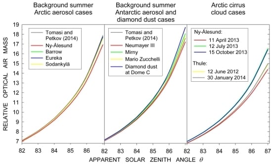
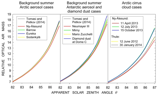
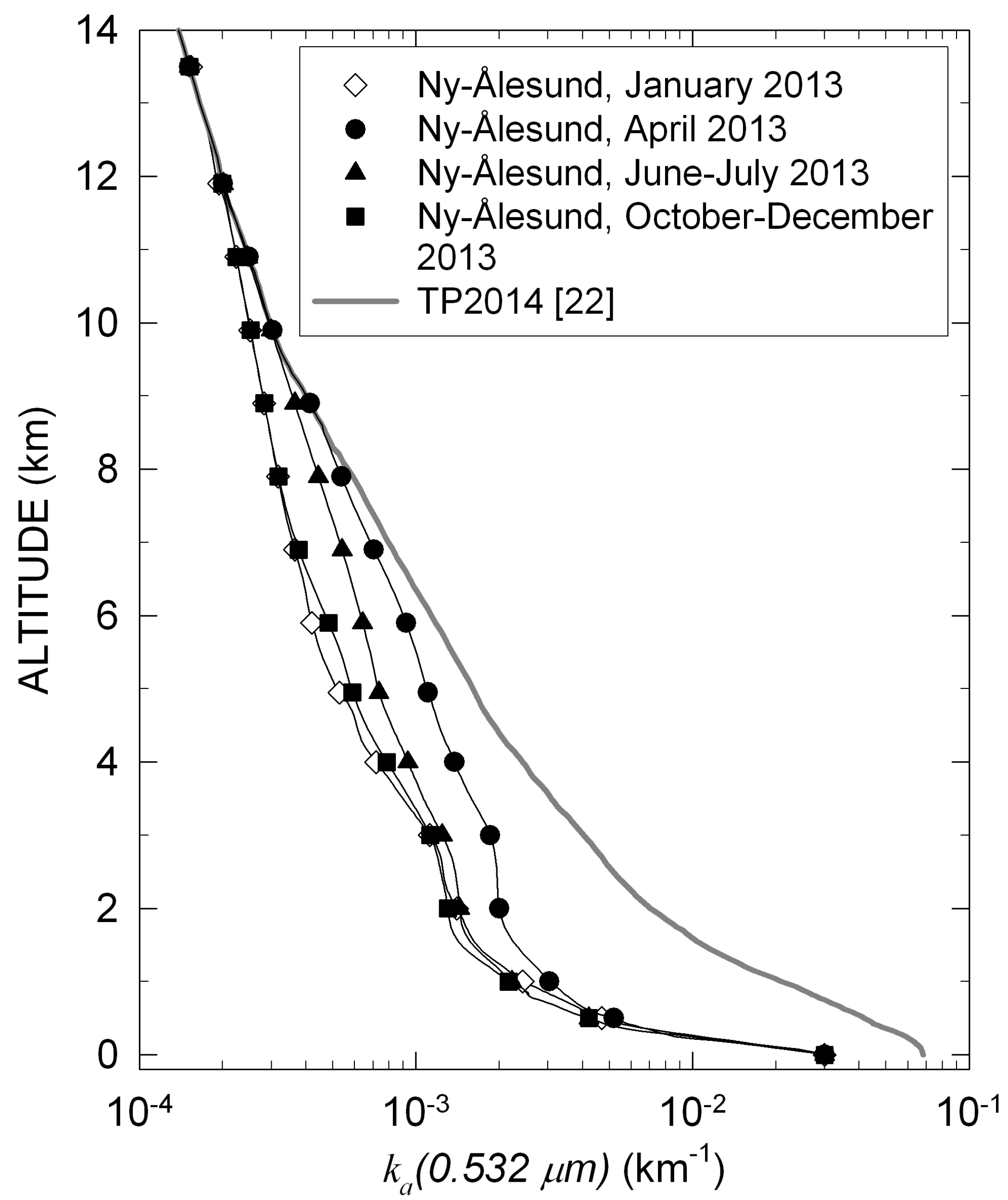
3.1. Background Arctic Aerosol Cases based on the Koldewey-Aerosol-Raman Lidar-System Measurements at Ny-Ålesund

Monthly mean vertical profiles of aerosol extinction coefficient k_a(z) measured with the KARL lidar in four different periods of the year are shown in Figure 2. As discussed above, k_a(z) is calculated from the measured values of B_bs(0.532 μm) using appropriate values of the lidar ratio [1].

Figure 2. Monthly or multi-monthly average vertical profiles of aerosol volume extinction coefficient k_a(0.532 μm) determined from the corresponding monthly or multi-monthly average vertical profiles of aerosol volume backscatter coefficient B_bs(0.532 μm) determined by Tomasi et al. [1] and obtained from the AWI KARL lidar system measurements conducted at Ny-Ålesund (~79°N, Spitsbergen, Svalbard) in January, April, June–July and October−December 2013. Note that the ground-level visual range V₀ assumed by TP2014 [22] at Ny-Ålesund for the vertical profile of k_a(0.532 μm) is equal to 50 km, while that assumed in the present study for all the four monthly (or multi-monthly) mean vertical profiles of k_a(0.532 μm) obtained from the field measurements is equal to 90 km.

Figure 2. Monthly or multi-monthly average vertical profiles of aerosol volume extinction coefficient k_a(0.532 μm) determined from the corresponding monthly or multi-monthly average vertical profiles of aerosol volume backscatter coefficient B_bs(0.532 μm) determined by Tomasi et al. [1] and obtained from the AWI KARL lidar system measurements conducted at Ny-Ålesund (~79°N, Spitsbergen, Svalbard) in January, April, June–July and October−December 2013. Note that the ground-level visual range V₀ assumed by TP2014 [22] at Ny-Ålesund for the vertical profile of k_a(0.532 μm) is equal to 50 km, while that assumed in the present study for all the four monthly (or multi-monthly) mean vertical profiles of k_a(0.532 μm) obtained from the field measurements is equal to 90 km.

The values of k_a(0.532 μm) at all the tropospheric levels are appreciably lower than those calculated by TP2014 [22] or the summer background Arctic aerosol at Ny-Ålesund, yielding a ground-level visual range V₀ = 50 km (calculated according to the Koschmieder theory [36]) The monthly mean vertical profiles of k_a(0.532 μm) determined in January, April, June-July and October–December are shown in Figure 2. They provide a value of V₀ = 90 km in all cases. Therefore, the dataset pertains to considerably higher atmospheric transmittance conditions in the visible than those assumed by TP2014 [22]. In fact, the extinction coefficients of the four monthly or multi-monthly mean vertical profiles of k_a(0.532 μm) in Figure 2 are appreciably lower than those defined for the summer background Arctic aerosol for z < 8 km. In particular, the vertical profiles determined in January and October–December are very similar, with values of k_a(0.532 μm) decreasing from 10⁻³ to 3 × 10⁻⁴ km⁻¹ as z increases from 3 to 10 km. Appreciably higher values were measured in June−July, mainly in the upper troposphere; this profile more typically represents the summer background aerosol vertical distribution. The highest values of k_a(0.532 μm) are found in April at all the tropospheric levels, presumably due to the frequent episodes of Arctic haze observed in early spring at this site. The KARL mean vertical profiles of k_a(0.532 μm) were determined up to levels varying between 8.5 and 12 km from the lidar observations, and were completed up to 50 km altitude with the extinction coefficient data determined by TP2014 [22] for summer background Arctic aerosol. The values of τ_a(0.532 μm) were equal to 0.016 in January, 0.020 in April, 0.017 in June–July and 0.015 in October–December, therefore considerably less than the value of Arctic summer background aerosol optical thickness τ_baa(0.532 μm) = 0.072 determined by TP2014 [22] for the average summer background Arctic aerosols.

In order to obtain reliable estimates of m_a(θ), the vertical profiles of k_a(0.532 μm) shown in Figure 2 were extended to the whole stratospheric altitude range with the vertical profiles defined by TP2014 [22]. These were derived from KARL lidar measurements performed at Ny-Ålesund in summer 2009 over the 12–50 km altitude range, and are representative of background Arctic aerosol without volcanic particles in the lower stratosphere. The values of m_a(θ), calculated using the four complete vertical profiles of k_a(0.532 μm) from the surface to 50 km height, are given in Table 2. They are appreciably lower than the values of Arctic summer background relative optical air mass m_baa(θ) calculated by TP2014 [22]. The differences are equal to about −1% at around θ = 82° for January, at about θ = 81° for April and June–July, and at θ = 82° for October–December, and are at θ = 87° equal to about −4% in January and October–December (corresponding to values of τ_a(0.532 μm) close to 0.015) and nearly equal to −6% in April and June–July for slightly higher values of τ_a(0.532 μm). This shows that the present estimates of m_a(θ) are lower by 4% to 6% than those given by TP2014 [22], being associated with values of τ_a(0.532 μm) ranging between 0.015 and 0.020, which are considerably lower than τ_baa(0.532 μm).

Table 2. Values of the relative optical air mass functions m_a(θ) calculated for 25 selected values of apparent solar zenith angle θ ranging from 0° to 87°, as obtained in the present study for background summer Arctic aerosol using as weight functions in Equation (3) the average vertical profiles of k_a(z) shown in Figure 2 for Ny-Ålesund in April, June–July and October of 2013, and in Figure 3 for Barrow, Eureka, and Sodankylä, obtained by averaging the CALIPSO data collected during the summer months from June to October of the last 2 years. The present results are compared with the TP2014 [22] evaluations of relative optical air mass function m_baa(θ) determined at Ny-Ålesund for background Arctic aerosol in summer, which are reported in the last column for comparison.

θ (°)	Ny-Ålesund				Barrow	Eureka	Sodankylä	Tomasi and Petkov [22]
	January Average	April Average	June-July Average	October−December Average	Summer Average	Summer Average	Summer Average	mbaa(θ)
0	1.0000	1.0000	1.0000	1.0000	1.0000	1.0000	1.0000	1.0000
10	1.0154	1.0154	1.0154	1.0154	1.0154	1.0154	1.0154	1.0154
20	1.0641	1.0641	1.0641	1.0641	1.0641	1.0641	1.0641	1.0641
30	1.1545	1.1545	1.1545	1.1545	1.1546	1.1546	1.1546	1.1546
40	1.3050	1.3049	1.3049	1.3050	1.3051	1.3051	1.3051	1.3052
50	1.5547	1.5546	1.5546	1.5546	1.5551	1.5551	1.5550	1.5552
55	1.7418	1.7417	1.7416	1.7417	1.7424	1.7424	1.7423	1.7426
60	1.9972	1.9970	1.9969	1.9971	1.9982	1.9983	1.9981	1.9986
65	2.3611	2.3608	2.3606	2.3609	2.3630	2.3631	2.3628	2.3636
70	2.9135	2.9129	2.9126	2.9131	2.9173	2.9176	2.9169	2.9186
72	3.2218	3.2210	3.2206	3.2213	3.2271	3.2274	3.2265	3.2288
74	3.6076	3.6064	3.6058	3.6068	3.6151	3.6156	3.6143	3.6175
75	3.8389	3.8375	3.8368	3.8380	3.8481	3.8487	3.8471	3.8510
76	4.1031	4.1014	4.1005	4.1020	4.1144	4.1151	4.1131	4.1179
77	4.4075	4.4052	4.4041	4.4061	4.4214	4.4223	4.4198	4.4259
78	4.7617	4.7588	4.7574	4.7599	4.7793	4.7804	4.7772	4.7849
79	5.1789	5.1750	5.1733	5.1765	5.2014	5.2029	5.1988	5.2087
80	5.6771	5.6718	5.6697	5.6739	5.7065	5.7086	5.7030	5.7162
81	6.2820	6.2745	6.2717	6.2776	6.3213	6.3242	6.3166	6.3344
82	7.0311	7.0201	7.0165	7.0249	7.0852	7.0894	7.0786	7.1035
83	7.9817	7.9647	7.9601	7.9725	8.0586	8.0653	8.0490	8.0853
84	9.2259	9.1978	9.1921	9.2115	9.3395	9.3507	9.3248	9.3804
85	10.921	10.870	10.864	10.897	11.097	11.117	11.073	11.163
86	13.358	13.257	13.254	13.314	13.647	13.690	13.604	13.765
87	17.149	16.917	16.934	17.061	17.657	17.765	17.571	17.893

Table 2. Values of the relative optical air mass functions m_a(θ) calculated for 25 selected values of apparent solar zenith angle θ ranging from 0° to 87°, as obtained in the present study for background summer Arctic aerosol using as weight functions in Equation (3) the average vertical profiles of k_a(z) shown in Figure 2 for Ny-Ålesund in April, June–July and October of 2013, and in Figure 3 for Barrow, Eureka, and Sodankylä, obtained by averaging the CALIPSO data collected during the summer months from June to October of the last 2 years. The present results are compared with the TP2014 [22] evaluations of relative optical air mass function m_baa(θ) determined at Ny-Ålesund for background Arctic aerosol in summer, which are reported in the last column for comparison.

θ (°)	Ny-Ålesund				Barrow	Eureka	Sodankylä	Tomasi and Petkov [22]
	January Average	April Average	June-July Average	October−December Average	Summer Average	Summer Average	Summer Average	mbaa(θ)
0	1.0000	1.0000	1.0000	1.0000	1.0000	1.0000	1.0000	1.0000
10	1.0154	1.0154	1.0154	1.0154	1.0154	1.0154	1.0154	1.0154
20	1.0641	1.0641	1.0641	1.0641	1.0641	1.0641	1.0641	1.0641
30	1.1545	1.1545	1.1545	1.1545	1.1546	1.1546	1.1546	1.1546
40	1.3050	1.3049	1.3049	1.3050	1.3051	1.3051	1.3051	1.3052
50	1.5547	1.5546	1.5546	1.5546	1.5551	1.5551	1.5550	1.5552
55	1.7418	1.7417	1.7416	1.7417	1.7424	1.7424	1.7423	1.7426
60	1.9972	1.9970	1.9969	1.9971	1.9982	1.9983	1.9981	1.9986
65	2.3611	2.3608	2.3606	2.3609	2.3630	2.3631	2.3628	2.3636
70	2.9135	2.9129	2.9126	2.9131	2.9173	2.9176	2.9169	2.9186
72	3.2218	3.2210	3.2206	3.2213	3.2271	3.2274	3.2265	3.2288
74	3.6076	3.6064	3.6058	3.6068	3.6151	3.6156	3.6143	3.6175
75	3.8389	3.8375	3.8368	3.8380	3.8481	3.8487	3.8471	3.8510
76	4.1031	4.1014	4.1005	4.1020	4.1144	4.1151	4.1131	4.1179
77	4.4075	4.4052	4.4041	4.4061	4.4214	4.4223	4.4198	4.4259
78	4.7617	4.7588	4.7574	4.7599	4.7793	4.7804	4.7772	4.7849
79	5.1789	5.1750	5.1733	5.1765	5.2014	5.2029	5.1988	5.2087
80	5.6771	5.6718	5.6697	5.6739	5.7065	5.7086	5.7030	5.7162
81	6.2820	6.2745	6.2717	6.2776	6.3213	6.3242	6.3166	6.3344
82	7.0311	7.0201	7.0165	7.0249	7.0852	7.0894	7.0786	7.1035
83	7.9817	7.9647	7.9601	7.9725	8.0586	8.0653	8.0490	8.0853
84	9.2259	9.1978	9.1921	9.2115	9.3395	9.3507	9.3248	9.3804
85	10.921	10.870	10.864	10.897	11.097	11.117	11.073	11.163
86	13.358	13.257	13.254	13.314	13.647	13.690	13.604	13.765
87	17.149	16.917	16.934	17.061	17.657	17.765	17.571	17.893

3.2. Background Summer Arctic Aerosol Cases based on the Cloud-Aerosol Lidar and Infrared Pathfinder Satellite Observations over Barrow, Eureka and Sodankylä

The seasonal average vertical profiles of k_a(0.532 μm) shown in Figure 3a were derived from the CALIOP/CALIPSO satellite datasets collected in summer during 2013 and 2014 at Barrow, Eureka and Sodankylä. As above, these profiles were used as weighting functions in Equation (3). It is interesting to note that k_a(0.532 μm) is significantly smaller than the values given by TP2014 [22] in the lowest two kilometers. In particular, very similar values of k_a(0.532 μm) were determined at the surface at Barrow and Sodankylä, corresponding to values of V₀ of 57 and 60 km, respectively. At both sites k_a(0.532 μm) slowly decreases with altitude until reaching the TP2014 [22] profile at about 2 km altitude. Conversely, the vertical profile of k_a(0.532 μm) at Eureka displays values considerably lower than those of Barrow and Sodankylä at z < ~2 km, the surface-level value yielding V₀ = 56 km. The vertical profile of k_a(0.532 μm) was completed above the 5 km level with a profile typical of background polar aerosol, which remains stable at Eureka, Ny-Ålesund and Sodankylä during the summer months, as shown by the lidar measurements conducted at these Arctic sites. On the basis of these measurements, we assumed that k_a(0.532 μm) gradually increases with height to reach the TP2014 [22] rofile at about 5-km altitude. The three CALIPSO vertical profiles of k_a(0.532 μm) shown in Figure 3a were then extended up to 50 km altitude by using the summer background Arctic aerosol profile defined by TP2014 [22] in the upper part of the troposphere and the whole stratosphere. The corresponding summer average values of τ_a(0.532 μm) were 0.053 at Barrow, 0.045 at Eureka, and 0.046 at Sodankylä, which are all considerably lower than the TP2014 [22] value of τ_baa(0.532 μm) equal to 0.072 for atmospheric turbidity conditions typical of background Arctic aerosol in summer.

Figure 3. Left-hand side (a): Seasonal mean vertical profiles of aerosol volume extinction coefficient k_a(0.532 μm) determined from daily CALIPSO measurements of volume aerosol backscattering coefficient B_bs(0.532 μm) conducted at Barrow (~71°N), Eureka (~80°N) and Sodankylä (~67°N) during the summer (June-September) months of 2013 and 2014. Right-hand side (b): As in the left-hand side, for the sets of CALIPSO measurements conducted at Neumayer III (~71°S), Mirny (~67°S) and Mario Zucchelli (~75°S), Terra Nova Bay, Ross Sea) in Antarctica during the austral summer (November–February) months of 2013 and 2014.

Figure 3. Left-hand side (a): Seasonal mean vertical profiles of aerosol volume extinction coefficient k_a(0.532 μm) determined from daily CALIPSO measurements of volume aerosol backscattering coefficient B_bs(0.532 μm) conducted at Barrow (~71°N), Eureka (~80°N) and Sodankylä (~67°N) during the summer (June-September) months of 2013 and 2014. Right-hand side (b): As in the left-hand side, for the sets of CALIPSO measurements conducted at Neumayer III (~71°S), Mirny (~67°S) and Mario Zucchelli (~75°S), Terra Nova Bay, Ross Sea) in Antarctica during the austral summer (November–February) months of 2013 and 2014.

The values of m_a(θ) calculated using these three CALIPSO vertical profiles of k_a(0.532 μm) are given in Table 2, for comparison with the values of m_a(θ) determined from the KARL measurements at Ny-Ålesund, and with those of m_baa(θ) by TP2014 [22]. The comparison indicates that the CALIPSO-derived values of m_a(θ) at the three Arctic sites gradually increase as a function of solar zenith angle θ differing only slightly from those calculated by TP2014 [22]. The percent differences at θ = 87° are −1.3% at Barrow, −0.7% at Eureka, and −1.8% at Sodankylä. These small discrepancies can be plausibly attributed to the relatively lower values of τ_a(0.532 μm) obtained for the CALIPSO observations, which are 26%, 37% and 36% lower than τ_baa(0.532 μm).

3.3. Background Austral Summer Antarctic Aerosol Cases at Neumayer III, Mirny and Mario Zucchelli from CALIPSO Observations

The calculations of m_a(θ) for the three Antarctic coastal sites were carried out as explained in the previous section, using the average vertical profiles of k_a(0.532 μm) derived from the CALIOP/CALIPSO observations made in the summer months of 2013 and 2014, and shown in Figure 3b. Reliable values of k_a(0.532 μm) were found only in the lowest atmospheric layers, approximately below 1.4 km. The ground-level extinction coefficient values correspond to values of V₀ equal to 42 km at Mirny, 72 km at Mario Zucchelli, and largely more than 100 km at Neumayer III. At all these sites, the sea salt aerosols, generated by winds over the ocean surfaces and then transported toward the coastal regions [7], are the predominant particulate constituent in the boundary layer. The vertical profiles of k_a(0.532 μm) shown in Figure 3b were completed with the TP2014 [22] vertical profile of summer background Antarctic aerosol over the altitude range from ~1.5 to 50 km. The corresponding average values of τ_a(0.532 μm) were evaluated to be equal to 0.026 at Neumayer III, 0.057 at Mirny, and 0.042 at Mario Zucchelli. Among these mean values of τ_a(0.532 μm), the estimate obtained at Neumayer III is therefore lower by 26% than the value of 0.035 estimated by TP2014 [22] for austral summer background Antarctic aerosol at coastal sites over the altitude range from the surface to the stratopause-level, and those here determined at Mirny and Mario Zucchelli are higher by 63% and 20%, respectively, than the value of τ_bAa(0.532 μm) calculated by TP2014 [22].

The summer average values of m_a(θ) were calculated for the vertical profiles of k_a(0.532 μm) at the three sites. The results are given in Table 3 for θ ranging from 0° to 87°. The comparison with the values of m_bAa(θ) determined by TP2014 [22] for austral summer background Antarctic aerosol at coastal sites indicates that the values of m_a(θ) determined at Neumayer III are slightly lower than m_bAa(θ) by ~1% at θ = 85° and ~2% at θ = 87°. The value of τ_a(0.532 μm) at Neumayer III is 0.026, which is equal to about 74% of τ_bAa(0.532 μm). Conversely, m_a(θ) evaluated at Mirny is higher than m_bAa(θ) by ~1% at θ = 84.5° and nearly 3% at θ = 87°. The value of τ_a(0.532 μm) is equal to 0.057, which is 63% higher than τ_bAa(0.532 μm), suggesting that higher values of m_a(θ) are associated with higher values of τ_a(0.532 μm). The Mario Zucchelli values of m_a(θ) are slightly higher by about 1% than m_bAa(θ) for θ = 87°, for the value of τ_a(0.532 μm) which is 20% higher than τ_bAa(0.532 μm).

Table 3. Values of the relative optical air mass functions m_a(θ) calculated for 25 selected values of apparent solar zenith angle θ ranging from 0° to 87°, as obtained in the present study for background summer Antarctic aerosol used as weight functions in Equation (3) the average vertical profiles of k_a(z) shown in Figure 3b for Neumayer III, Mirny and Mario Zucchelli, as obtained by averaging the CALIPSO data collected during the summer months from November to February of the last 2 years, and values of the relative optical air mass functions m_dd(θ) calculated for diamond dust particles obtained for the average vertical profile of k_a(0.532 μm) shown in Figure 4 for a diamond dust ground layer observed at Dome C on 7 February 2008 (00:40 UTC) using the INO-CNR Antarctic lidar. The present results are compared with the TP2014 [22] evaluations of relative optical air mass function m_bAa(θ) determined at Mario Zucchelli for background Antarctic aerosol in austral summer, which are reported in the last column for comparison.

θ (°)	Summer background Antarctic Aerosol ma(θ)			Diamond Dust Case	Tomasi and Petkov [22]
	Neumayer III (Seasonal Average)	Mirny (Seasonal Average)	Mario Zucchelli (Seasonal Average)	mdd(θ)	mbAa(θ)
0	1.0000	1.0000	1.0000	1.0000	1.0000
10	1.0154	1.0154	1.0154	1.0154	1.0154
20	1.0641	1.0641	1.0641	1.0642	1.0641
30	1.1545	1.1546	1.1546	1.1547	1.1546
40	1.3050	1.3052	1.3052	1.3053	1.3051
50	1.5548	1.5553	1.5551	1.5555	1.5550
55	1.7420	1.7427	1.7425	1.7431	1.7423
60	1.9976	1.9987	1.9983	1.9995	1.9981
65	2.3618	2.3639	2.3632	2.3652	2.3627
70	2.9149	2.9192	2.9178	2.9219	2.9168
72	3.2238	3.2297	3.2277	3.2334	3.2263
74	3.6104	3.6188	3.6160	3.6241	3.6140
75	3.8423	3.8525	3.8491	3.8591	3.8467
76	4.1072	4.1198	4.1156	4.1279	4.1126
77	4.4125	4.4282	4.4230	4.4383	4.4193
78	4.7680	4.7879	4.7813	4.8007	4.7766
79	5.1869	5.2126	5.2040	5.2292	5.1980
80	5.6874	5.7213	5.7101	5.7434	5.7020
81	6.2955	6.3415	6.3262	6.3716	6.3153
82	7.0493	7.1137	7.0922	7.1561	7.0770
83	8.0067	8.1006	8.0691	8.1630	8.0471
84	9.2609	9.4047	9.3564	9.5017	9.3226
85	10.970	11.205	11.126	11.367	11.071
86	13.426	13.846	13.703	14.146	13.605
87	17.223	18.075	17.780	18.720	17.584

Table 3. Values of the relative optical air mass functions m_a(θ) calculated for 25 selected values of apparent solar zenith angle θ ranging from 0° to 87°, as obtained in the present study for background summer Antarctic aerosol used as weight functions in Equation (3) the average vertical profiles of k_a(z) shown in Figure 3b for Neumayer III, Mirny and Mario Zucchelli, as obtained by averaging the CALIPSO data collected during the summer months from November to February of the last 2 years, and values of the relative optical air mass functions m_dd(θ) calculated for diamond dust particles obtained for the average vertical profile of k_a(0.532 μm) shown in Figure 4 for a diamond dust ground layer observed at Dome C on 7 February 2008 (00:40 UTC) using the INO-CNR Antarctic lidar. The present results are compared with the TP2014 [22] evaluations of relative optical air mass function m_bAa(θ) determined at Mario Zucchelli for background Antarctic aerosol in austral summer, which are reported in the last column for comparison.

θ (°)	Summer background Antarctic Aerosol ma(θ)			Diamond Dust Case	Tomasi and Petkov [22]
	Neumayer III (Seasonal Average)	Mirny (Seasonal Average)	Mario Zucchelli (Seasonal Average)	mdd(θ)	mbAa(θ)
0	1.0000	1.0000	1.0000	1.0000	1.0000
10	1.0154	1.0154	1.0154	1.0154	1.0154
20	1.0641	1.0641	1.0641	1.0642	1.0641
30	1.1545	1.1546	1.1546	1.1547	1.1546
40	1.3050	1.3052	1.3052	1.3053	1.3051
50	1.5548	1.5553	1.5551	1.5555	1.5550
55	1.7420	1.7427	1.7425	1.7431	1.7423
60	1.9976	1.9987	1.9983	1.9995	1.9981
65	2.3618	2.3639	2.3632	2.3652	2.3627
70	2.9149	2.9192	2.9178	2.9219	2.9168
72	3.2238	3.2297	3.2277	3.2334	3.2263
74	3.6104	3.6188	3.6160	3.6241	3.6140
75	3.8423	3.8525	3.8491	3.8591	3.8467
76	4.1072	4.1198	4.1156	4.1279	4.1126
77	4.4125	4.4282	4.4230	4.4383	4.4193
78	4.7680	4.7879	4.7813	4.8007	4.7766
79	5.1869	5.2126	5.2040	5.2292	5.1980
80	5.6874	5.7213	5.7101	5.7434	5.7020
81	6.2955	6.3415	6.3262	6.3716	6.3153
82	7.0493	7.1137	7.0922	7.1561	7.0770
83	8.0067	8.1006	8.0691	8.1630	8.0471
84	9.2609	9.4047	9.3564	9.5017	9.3226
85	10.970	11.205	11.126	11.367	11.071
86	13.426	13.846	13.703	14.146	13.605
87	17.223	18.075	17.780	18.720	17.584

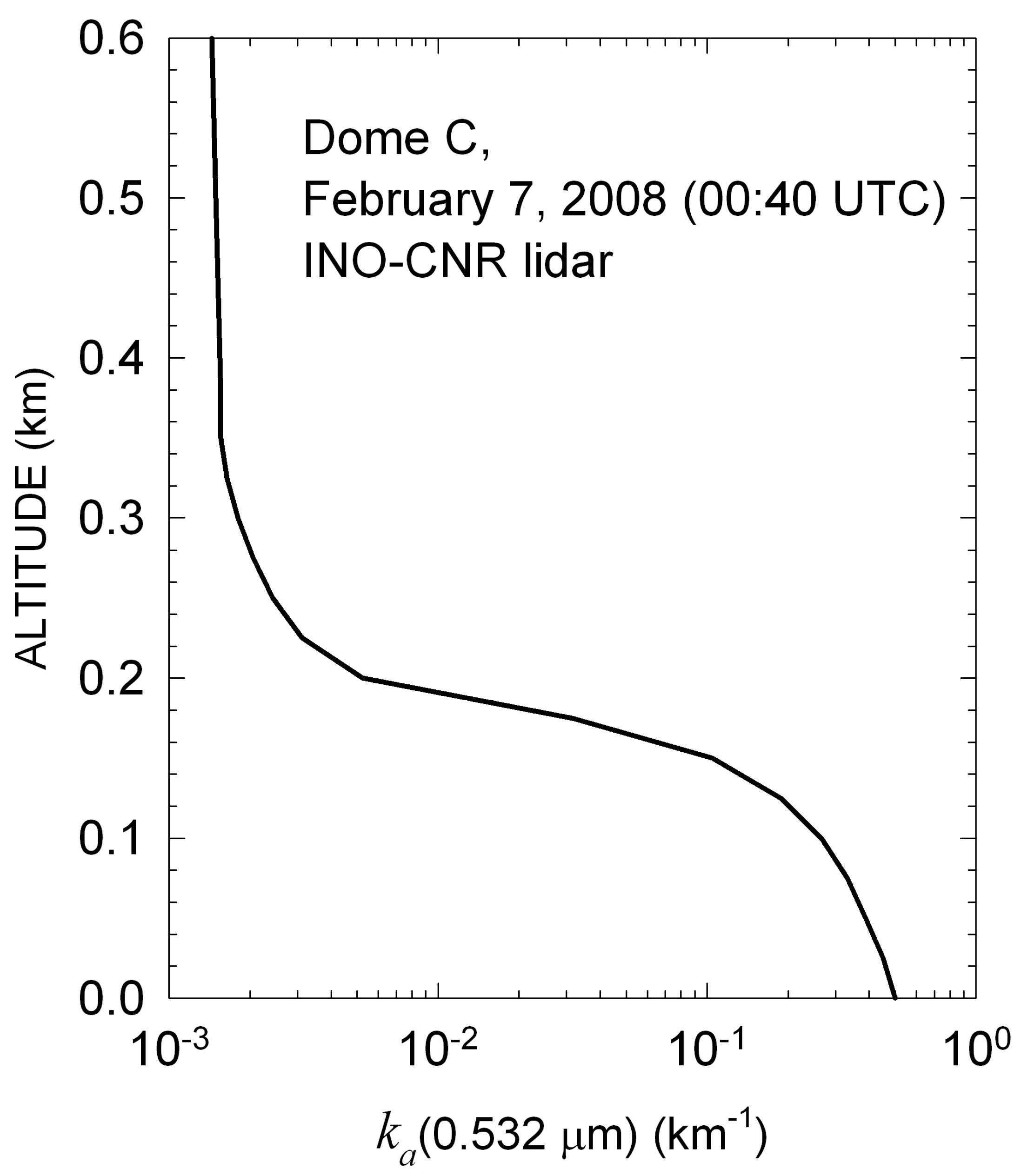
3.4. A Diamond Dust Case at Dome C from National Institute of Optics (INO), National Council of Research (CNR) Antarctic Lidar Measurements

Tomasi et al. [6] have shown that many diamond dust episodes occur at Amundsen-Scott South Pole base (89°59'S, 139°16'E, 2835 m a.m.s.l.), examining the spectral series of aerosol optical thickness τ_a(λ) carried out at visible and near-infrared wavelengths by Global Monitoring Division (GMD)/National Oceanic and Atmospheric Administration (NOAA) [9] using the SP02 Carter Scott sun-photometers. The values of τ_a(0.500 μm) were found to vary mainly from less than 0.02 to 0.08 and the values of the Ångström [37] exponent α range from less than 0.3 to about 1.2. The low values of α are often due to the presence of significant concentrations of diamond dust particles near the ground. The mobilization of diamond dust by winds is also very frequently observed at the Dome C base on the Eastern Antarctic Plateau, as confirmed by the INO-CNR Antarctic lidar observations. Diamond dust particles are often present in the lowest 100–200 m of the atmosphere, with values of k_a(0.532 μm) decreasing with height. Background values typical of the free troposphere are reached at 400–500 m altitude. A sharp increase in the particulate extinction at the ground level is usually observed during these events. In these cases, specific estimates of air mass function m_dd(θ) are needed to analyze the sun-photometer measurements of direct solar irradiance for these particularly dense optical turbidity conditions. For this purpose, a diamond dust event observed at Dome C with the INO-CNR Antarctic lidar on 7 February 2008 (from 00:30 to 01:20 UTC) is considered here. The vertical profile of k_a(0.532 μm) is shown in Figure 4. The volume extinction coefficient k_a(0.532 μm) decreases slowly with height in the first 120–140 m above the surface, and rapidly above reaching values typical of the diamond dust-free upper troposphere at altitudes z > 0.4 km. The measured vertical profile of k_a(0.532 μm) up to the altitude of 0.4 km was connected with the austral summer background aerosol profile by TP2014 [22]. The overall value of τ_dd(0.532 μm) is 0.056, and the ground-level visual range is 7.7 km.

Figure 4. Vertical profile of volume aerosol extinction coefficient k_a(0.532 μm) obtained from the INO-CNR lidar measurements conducted at Dome C on 7 February 2008 (00:40 UTC). The relatively large values of the measured backscattering coefficient B_bs(0.532 μm) close to the ground is due to wind-mobilized diamond dust particles. The corresponding visual range V₀ is 7.7 km and the overall value of the aerosol optical thickness τ_a(0.55 μm) is 0.056.

Figure 4. Vertical profile of volume aerosol extinction coefficient k_a(0.532 μm) obtained from the INO-CNR lidar measurements conducted at Dome C on 7 February 2008 (00:40 UTC). The relatively large values of the measured backscattering coefficient B_bs(0.532 μm) close to the ground is due to wind-mobilized diamond dust particles. The corresponding visual range V₀ is 7.7 km and the overall value of the aerosol optical thickness τ_a(0.55 μm) is 0.056.

The values of relative optical air mass function m_dd(θ) for the diamond dust case are given in Table 3. The values of m_dd(θ) are appreciably higher than those of TP2014 [22] pertaining to background Antarctic austral summer aerosol, with differences exceeding + 1% for θ ≈ 81.5°, and up to about + 6.5% for θ = 87°. Such high values of m_dd(θ) are attributed to the higher aerosol optical thickness, with τ_dd(0.532 μm) about 60% higher than τ_bAa(0.532 μm). The present results show that the diamond dust extinction involving the lowest atmospheric layer implies a marked increase of the sun-path length through the ground layer. Therefore, the values of m_dd(θ) are in general expected to vary proportionally to the increase of τ_dd(0.532 μm), associated with the decrease in the ground-level visual range.

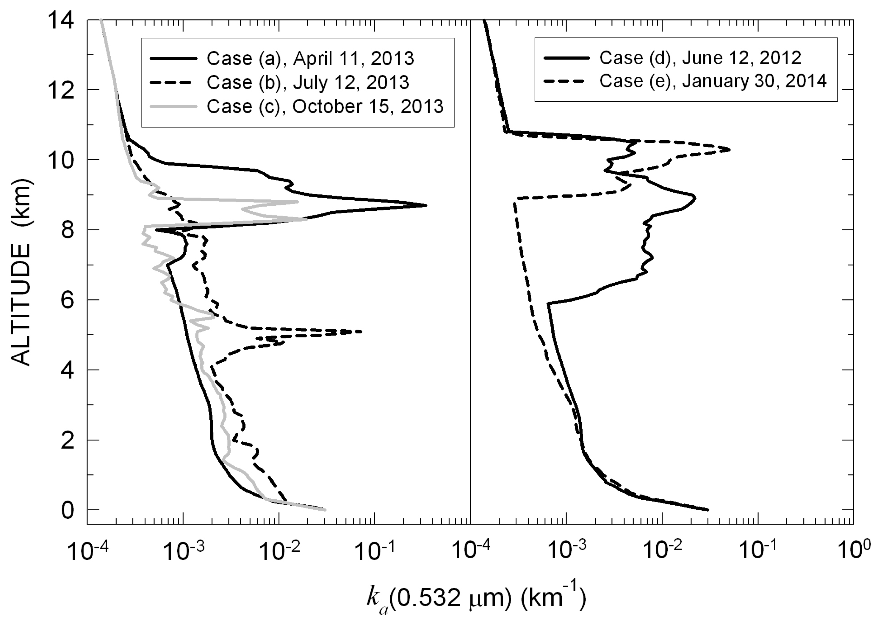
3.5. Various Tropospheric Cirrus Cloud Cases from Lidar Measurements at Ny-Ålesund and Thule

Five vertical profiles of k_a(0.532 μm) were considered to calculate the relative optical air mass function for cirrus clouds, m_cc(θ). The following cirrus cloud cases, whose profiles are shown in Figure 5, were selected:

Figure 5. Left-hand side: Vertical profiles of volume extinction coefficient k_a(0.532 μm) obtained from the KARL lidar measurements conducted at Ny-Ålesund (~79°N) for thin cirrus clouds at various tropospheric altitudes and measured on 11 April (15:10 UTC) (case (a)), 12 July (14:49 UTC) (case (b)), and 15 October (12:49 UTC) (case (c)). Each of these three profiles was superimposed to the corresponding monthly (or multi-monthly) mean vertical profile of k_a(0.532 μm) shown in Figure 2 obtained from the KARL lidar measurements conducted in April, June−July and October–December 2013, respectively. Right-hand side: as in the left-hand side, but for the vertical profiles of k_a(0.532 μm) derived from the University of Rome/ENEA lidar measurements conducted at Thule (~77°N) on June 12, 2012 (from 11:09 to 12:14 UTC) (case (d)) and January 30, 2014 (from 19:12 to 20:42 UTC) (case (e)). The cirrus cloud profiles were superimposed over the corresponding monthly or bi-monthly mean vertical profile of coefficient k_a(0.532 μm) shown in Figure 2 for June–July 2013 in case (d) and for January 2013 in case (e).

Figure 5. Left-hand side: Vertical profiles of volume extinction coefficient k_a(0.532 μm) obtained from the KARL lidar measurements conducted at Ny-Ålesund (~79°N) for thin cirrus clouds at various tropospheric altitudes and measured on 11 April (15:10 UTC) (case (a)), 12 July (14:49 UTC) (case (b)), and 15 October (12:49 UTC) (case (c)). Each of these three profiles was superimposed to the corresponding monthly (or multi-monthly) mean vertical profile of k_a(0.532 μm) shown in Figure 2 obtained from the KARL lidar measurements conducted in April, June−July and October–December 2013, respectively. Right-hand side: as in the left-hand side, but for the vertical profiles of k_a(0.532 μm) derived from the University of Rome/ENEA lidar measurements conducted at Thule (~77°N) on June 12, 2012 (from 11:09 to 12:14 UTC) (case (d)) and January 30, 2014 (from 19:12 to 20:42 UTC) (case (e)). The cirrus cloud profiles were superimposed over the corresponding monthly or bi-monthly mean vertical profile of coefficient k_a(0.532 μm) shown in Figure 2 for June–July 2013 in case (d) and for January 2013 in case (e).

(i) Case (a), relative to measurements made at Ny-Ålesund with the KARL lidar on 11 April 2013 (15:10 UTC). The vertical profile of k_a(0.532 μm) is characterized by a marked peak located at about 8.7 km. The cloud layer was superimposed to the monthly average vertical profile of k_a(0.532 μm) for April shown in Figure 2. The overall value of τ_cc(0.532 μm) is 0.098, i.e., about five times higher than the value of τ_a(0.532 μm) = 0.020 measured in April 2013, indicating that about 80% of the overall particulate extinction along the atmospheric path is produced by cloud particles, and only 20% by polar aerosols.

(ii) Case (b), from the KARL lidar measurements conducted at Ny-Ålesund on 12 July 2013 (14:49 UTC). The vertical profile is characterized by a marked peak centered at z ≈ 5 km, and significant extinction structures at other tropospheric levels. This profile has been assumed to be superimposed to the June−July 2013 average vertical profile of k_a(0.532 μm) shown in Figure 2. In this case, an overall value of τ_cc(0.532 μm) = 0.044 has been obtained, about five times higher than the June–July 2013 mean value of τ_a(0.532 μm) (= 0.017), indicating that about 60% of the overall atmospheric particulate extinction is due to cloud particles suspended in the middle troposphere.

(iii) Case (c), from the KARL lidar measurements conducted at Ny-Ålesund on 15 October 2013 (12:49 UTC). The measurements exhibit minor extinction features in the 2 to 6 km altitude range and a pronounced bicuspid maximum between 8 and 9 km, which has been assumed to be superimposed over the October–December 2013 average vertical profile shown in Figure 2. A value of τ_cc(0.532 μm) = 0.028 has been determined in this case, which is about twice the value of τ_a(0.532 μm) = 0.015, determined as October–December 2013 average at Ny-Ålesund, clearly indicating that about 46% of the overall particulate extinction is due to cloud particles.

(iv) Case (d), obtained from the University of Rome/ENEA lidar measurements conducted at Thule on 12 June 2012 over the time interval from 11:09 to 12:14 UTC. The profile shows a very marked multi-layered structure of thick cirrus clouds, extending from about 6 km to more than 10 km altitude, as can be seen in Figure 5. This lidar-derived profile was superimposed to the June−July average vertical profile shown in Figure 2 and assumed to be valid also at Thule. The overall value of τ_cc(0.532 μm) = 0.048 is considerably higher than the value of τ_a(0.532 μm) = 0.017 estimated for June–July 2013 at Ny-Ålesund. In this case, about 44% of the overall particulate extinction in the atmosphere is produced by cloud particles.

(v) Case (e), derived from the University of Rome/ENEA lidar measurements conducted at Thule on January 30, 2014, over the period from 19:12 to 20:42 UTC. Similarly to the previous cases, the monthly average aerosol profile at Ny-Ålesund for the month of January 2013, derived from the KARL lidar measurements, was added to the cirrus data. The obtained profile is shown in Figure 5. A marked extinction peak exists at z ≈ 10 km. The overall value of τ_cc(0.532 μm) was estimated in this case to be equal to 0.036, while a value of τ_a(0.532 μm) = 0.016 has been determined at Ny-Ålesund from the KARL lidar measurements conducted in January 2013, indicating that about 56% of the overall atmospheric particulate extinction is due to cloud particles and the remaining 44% to aerosols.

The values of m_cc(θ) were calculated for the above five cases by using in Equation (3) the composite vertical profiles of k_a(0.532 μm) shown in Figure 5 as weighting functions. The resulting values of m_cc(θ) are given in Table 4. The ratio m_cc(θ)/m_a(θ) is reported in Table 4 as a function of θ, to highlight the influence of the cirrus cloud layers shown in Figure 5. The values of m_a(θ) used in the ratio are derived from Table 2 for the Ny-Ålesund lidar observations made in April 2013 (for case (a)), June–July 2013 (for cases (b) and (d)), October−December 2013 (for case (c)) and January 2013 (for case (e)), respectively. It can be seen that the values of m_cc(θ) are 1% lower at θ = 76° for case (a), at θ ≈ 86° for case (b), at θ = 84° for case (c), at θ = 78° for case (d), and at θ = 77° for case (e). Considerably lower values of m_cc(θ) with respect to m_a(θ) were found for θ = 87°. The reduction is about 15% in case (a), 2% in case (b), 4% in case (c), 12% in case (d) and 13% in case (e). These results also provide evidence that the presence of cirrus clouds at mid and/or high tropospheric levels may lead to significant reductions of m_cc(θ) with respect to m_baa(θ), evaluated to increase with a rate proportional to the fraction of optical thickness due to cloud particles.

Table 4. Values of the relative optical air mass functions m_cc(θ) calculated for 25 selected values of apparent solar zenith angle θ ranging from 0° to 87°, as obtained using as weighting functions in Equation (3) the average vertical profiles of k_a(z) shown in Figure 5 for three thin cirrus cloud cases observed at Ny-Ålesund on 11 April (15:10 UTC) (case (a)), 12 July (14:49 UTC) (case (b)), and 15 October (12:49 UTC) (case (c)) using the KARL lidar system, and two cirrus cloud cases observed at Thule (76°39'N, 68°46'W, 225 m a.m.s.l.m.) on 12 June 2012 (from 11:09 to 12:14 UTC) (case (d)), and 30 January 2014 (from 19:12 to 20:42 UTC) (case (e)), using the Rome University LiDAR. The last five columns provide the values of ratios m_cc(θ)/m_a(θ) to give a measure of the percentage variations caused by the thin cirrus clouds with respect to the monthly mean values of m_a(θ) determined for background Arctic aerosol extinction features.

θ (°)	Thin Cirrus Clouds at Ny-Ålesund			Thin Cirrus Clouds at Thule		Ratios mcc(θ)/ma(θ)
	Case (a), 11 April 2013	Case (b), 12 July 2013	Case (c), 15 October 2013	Case (d), 12 June 2012	Case (e), 30 January 2014	Case (a)	Case (b)	Case (c)	Case (d)	Case (e)
0	1.0000	1.0000	1.0000	1.0000	1.0000	1.000	1.000	1.000	1.000	1.000
10	1.0154	1.0154	1.0154	1.0154	1.0154	1.000	1.000	1.000	1.000	1.000
20	1.0640	1.0641	1.0641	1.0640	1.0640	1.000	1.000	1.000	1.000	1.000
30	1.1543	1.1545	1.1545	1.1543	1.1543	1.000	1.000	1.000	1.000	1.000
40	1.3044	1.3049	1.3049	1.3045	1.3045	1.000	1.000	1.000	1.000	1.000
50	1.5533	1.5545	1.5544	1.5535	1.5534	0.999	1.000	1.000	0.999	0.999
55	1.7395	1.7415	1.7413	1.7399	1.7398	0.999	1.000	1.000	0.999	0.999
60	1.9933	1.9968	1.9964	1.9941	1.9938	0.998	1.000	1.000	0.999	0.998
65	2.3541	2.3604	2.3597	2.3555	2.3550	0.997	1.000	0.999	0.998	0.997
70	2.8995	2.9121	2.9106	2.9022	2.9013	0.995	1.000	0.999	0.996	0.996
72	3.2024	3.2199	3.2178	3.2061	3.2050	0.994	1.000	0.999	0.996	0.995
74	3.5797	3.6047	3.6018	3.5850	3.5834	0.993	1.000	0.999	0.994	0.993
75	3.8051	3.8355	3.8319	3.8115	3.8096	0.992	1.000	0.998	0.993	0.992
76	4.0614	4.0988	4.0944	4.0694	4.0671	0.990	1.000	0.998	0.992	0.991
77	4.3554	4.4020	4.3966	4.3653	4.3625	0.989	1.000	0.998	0.991	0.990
78	4.6955	4.7545	4.7478	4.7081	4.7046	0.987	0.999	0.997	0.990	0.988
79	5.0932	5.1694	5.1608	5.1095	5.1052	0.984	0.999	0.997	0.988	0.986
80	5.5636	5.6641	5.6529	5.5852	5.5798	0.981	0.999	0.996	0.985	0.983
81	6.1276	6.2636	6.2487	6.1570	6.1501	0.977	0.999	0.995	0.982	0.979
82	6.8142	7.0039	6.9837	6.8554	6.8467	0.971	0.998	0.994	0.977	0.974
83	7.6648	7.9395	7.9113	7.7249	7.7140	0.962	0.997	0.992	0.970	0.966
84	8.7394	9.1559	9.1153	8.8315	8.8186	0.950	0.996	0.990	0.961	0.956
85	10.126	10.794	10.734	10.276	10.264	0.932	0.994	0.985	0.946	0.940
86	11.954	13.102	13.014	12.217	12.218	0.902	0.989	0.977	0.922	0.915
87	14.401	16.551	16.432	14.910	14.980	0.851	0.977	0.963	0.880	0.873

Table 4. Values of the relative optical air mass functions m_cc(θ) calculated for 25 selected values of apparent solar zenith angle θ ranging from 0° to 87°, as obtained using as weighting functions in Equation (3) the average vertical profiles of k_a(z) shown in Figure 5 for three thin cirrus cloud cases observed at Ny-Ålesund on 11 April (15:10 UTC) (case (a)), 12 July (14:49 UTC) (case (b)), and 15 October (12:49 UTC) (case (c)) using the KARL lidar system, and two cirrus cloud cases observed at Thule (76°39'N, 68°46'W, 225 m a.m.s.l.m.) on 12 June 2012 (from 11:09 to 12:14 UTC) (case (d)), and 30 January 2014 (from 19:12 to 20:42 UTC) (case (e)), using the Rome University LiDAR. The last five columns provide the values of ratios m_cc(θ)/m_a(θ) to give a measure of the percentage variations caused by the thin cirrus clouds with respect to the monthly mean values of m_a(θ) determined for background Arctic aerosol extinction features.

θ (°)	Thin Cirrus Clouds at Ny-Ålesund			Thin Cirrus Clouds at Thule		Ratios mcc(θ)/ma(θ)
	Case (a), 11 April 2013	Case (b), 12 July 2013	Case (c), 15 October 2013	Case (d), 12 June 2012	Case (e), 30 January 2014	Case (a)	Case (b)	Case (c)	Case (d)	Case (e)
0	1.0000	1.0000	1.0000	1.0000	1.0000	1.000	1.000	1.000	1.000	1.000
10	1.0154	1.0154	1.0154	1.0154	1.0154	1.000	1.000	1.000	1.000	1.000
20	1.0640	1.0641	1.0641	1.0640	1.0640	1.000	1.000	1.000	1.000	1.000
30	1.1543	1.1545	1.1545	1.1543	1.1543	1.000	1.000	1.000	1.000	1.000
40	1.3044	1.3049	1.3049	1.3045	1.3045	1.000	1.000	1.000	1.000	1.000
50	1.5533	1.5545	1.5544	1.5535	1.5534	0.999	1.000	1.000	0.999	0.999
55	1.7395	1.7415	1.7413	1.7399	1.7398	0.999	1.000	1.000	0.999	0.999
60	1.9933	1.9968	1.9964	1.9941	1.9938	0.998	1.000	1.000	0.999	0.998
65	2.3541	2.3604	2.3597	2.3555	2.3550	0.997	1.000	0.999	0.998	0.997
70	2.8995	2.9121	2.9106	2.9022	2.9013	0.995	1.000	0.999	0.996	0.996
72	3.2024	3.2199	3.2178	3.2061	3.2050	0.994	1.000	0.999	0.996	0.995
74	3.5797	3.6047	3.6018	3.5850	3.5834	0.993	1.000	0.999	0.994	0.993
75	3.8051	3.8355	3.8319	3.8115	3.8096	0.992	1.000	0.998	0.993	0.992
76	4.0614	4.0988	4.0944	4.0694	4.0671	0.990	1.000	0.998	0.992	0.991
77	4.3554	4.4020	4.3966	4.3653	4.3625	0.989	1.000	0.998	0.991	0.990
78	4.6955	4.7545	4.7478	4.7081	4.7046	0.987	0.999	0.997	0.990	0.988
79	5.0932	5.1694	5.1608	5.1095	5.1052	0.984	0.999	0.997	0.988	0.986
80	5.5636	5.6641	5.6529	5.5852	5.5798	0.981	0.999	0.996	0.985	0.983
81	6.1276	6.2636	6.2487	6.1570	6.1501	0.977	0.999	0.995	0.982	0.979
82	6.8142	7.0039	6.9837	6.8554	6.8467	0.971	0.998	0.994	0.977	0.974
83	7.6648	7.9395	7.9113	7.7249	7.7140	0.962	0.997	0.992	0.970	0.966
84	8.7394	9.1559	9.1153	8.8315	8.8186	0.950	0.996	0.990	0.961	0.956
85	10.126	10.794	10.734	10.276	10.264	0.932	0.994	0.985	0.946	0.940
86	11.954	13.102	13.014	12.217	12.218	0.902	0.989	0.977	0.922	0.915
87	14.401	16.551	16.432	14.910	14.980	0.851	0.977	0.963	0.880	0.873

4. Conclusions

The multispectral sun-photometry method [18] requires accurate values of the relative optical air mass functions for Rayleigh scattering, aerosol, minor gases and thin clouds as a function of the apparent solar zenith angle θ (see Equations (1) and (2)). The calculations of m_a(θ) for Arctic and Antarctic cases of background polar aerosol made in this study indicate that for θ > 75° m_a(θ) appreciably decreases with respect to the TP2014 [22] estimates when τ_a(0.532 μm) is smaller than 0.07 at the Arctic sites and smaller than 0.03 at Antarctic sites. The present analysis of field data has demonstrated that m_a(θ) percent variations are proportional to the changes of aerosol optical thickness with respect to the background standard values. The percent changes of m_a(θ) become gradually larger as θ increases, up to θ = 87°, which constitutes the upper limit for rigorous sun-photometry applications.

The present results also provide evidence that the formation of an optically dense diamond dust layer near the surface, such as that shown in Figure 4, can cause a marked decrease in m_dd(θ) with respect to m_a(θ). The difference reaches several percent for θ > 80°. A pronounced relative increase exceeding 6% has been found for θ = 87° in the diamond dust case described in Figure 4. This large increase is attributed to the marked particulate extinction occurring within the lowest atmospheric layers, also involving the thermal and pressure characteristics of the ground layer and their effects on the air refractive index n(z).

Finally, five cases with cirrus cloud layers presenting different depths at various tropospheric altitudes were examined. The calculated values of the corresponding relative optical air mass function m_cc(θ) decrease for increasing θ with respect to m_a(θ) for pure background aerosol. The increase of m_cc(θ) with respect to m_a(θ) ranges from 2% to more than 10% as the overall optical thickness τ_cc(0.532 μm) increases from 0.028 to 0.098 because of the cirrus cloud contributions, which add to the pure background aerosol contribution, estimated to be equal to 0.02 on average at Dome C. In the five cases, the cirrus clouds produce an increment of the background aerosol optical thickness varying between 50% and about 80%, which enhances the effects of high-altitude pressure and temperature conditions observed at these high levels on both sun-path length and air refractive index, causing considerable decreases of m_cc(θ) with respect to m_baa(θ) for pure background aerosol.

References

1. Tomasi, C.; Kokhanovsky, A.A.; Lupi, A.; Ritter, C.; Smirnov, A.; O’Neill, N.T.; Stone, R.S.; Holben, B.N.; Nyeki, S.; Wehrli, C.; Stohl, A.; et al. Aerosol remote sensing in polar regions. Earth-Sci. Rev. 2015, 140, 108–157. [Google Scholar] [CrossRef] [Green Version]
2. Holben, B.N.; Eck, T.F.; Slutsker, I.; Tanré, D.; Buis, J.P.; Setzer, A.; Vermote, E.; Reagan, J.A.; Kaufman, Y.J.; Nakajima, T.; et al. AERONET—A federated instrument network and data archive for aerosol characterization. Remote Sens. Environ. 1998, 66, 1–16. [Google Scholar] [CrossRef]
3. Nakajima, T.; Yoon, S.C.; Ramanathan, V.; Shi, G.Y.; Takemura, T.; Higurashi, A.; Takamura, T.; Aoki, K.; Sohn, B.J.; Kim, S.W.; et al. Overview of the atmospheric brown cloud East Asian regional experiment 2005 and a study of the aerosol direct radiative forcing in East Asia. J. Geophys. Res. 2007, 112, D24S91. [Google Scholar]
4. Smirnov, A.; Holben, B.N.; Slutsker, I.; Giles, D.M.; McClain, C.R.; Eck, T.F.; Sakerin, S.M.; Macke, A.; Croot, P.; Zibordi, G.; et al. Maritime Aerosol Network as a component of Aerosol Robotic Network. J. Geophys. Res. 2009, 114, D06204. [Google Scholar]
5. Ohno, T. Aerosol routine observation operated by the Japan Meteorological Agency. In Proceedings of WMO/GAW Experts Workshop on a Global Surface-Based Network for Long Term Observations of Column Aerosol Optical Properties, Davos, Switzerland, 8–10 March 2004; pp. 70–71.
6. Tomasi, C.; Vitale, V.; Lupi, A.; Di Carmine, C.; Campanelli, M.; Herber, A.; Treffeisen, R.; Stone, R.S.; Andrews, E.; Sharma, S.; et al. Aerosols in polar regions: A historical overview based on optical depth and in situ observations. J. Geophys. Res. 2007, 112, D16205. [Google Scholar]
7. Tomasi, C.; Lupi, A.; Mazzola, M.; Stone, R.S.; Dutton, E.G.; Herber, A.; Vitale, V.; Radionov, V.F.; Holben, B.N.; Sorokin, M.G.; et al. An update of the long-term aerosol optical properties in polar regions using POLAR-AOD and other measurements performed during the International Polar Year. Atmos. Environ. 2012, 52, 29–47. [Google Scholar] [CrossRef] [Green Version]
8. Wehrli, C. Calibrations of filter radiometers for determination of atmospheric optical depths. Metrologia 2000, 37, 419–422. [Google Scholar] [CrossRef]
9. Stone, R.S. Monitoring aerosol optical depth at Barrow, Alaska, and South Pole; Historical overview, recent results and future goals. SIF Conf. Proc. 2002, 80, 123–144. [Google Scholar]
10. Shiobara, M.; Yamano, M.; Kobayashi, H.; Aoki, K.; Yabuki, M. Sky-radiometer measurement for monitoring column aerosol optical properties in Ny-Alesund—Recent results from the spring 2006–2007 measurements. In Proceedings of 8th Ny-Alesund Seminar, Cambridge, UK, 16–17 October 2007; pp. 32–35.
11. Di Carmine, C.; Campanelli, M.; Nakajima, T.; Tomasi, C.; Vitale, V. Retrievals of Antarctic aerosol characteristics using a Sun-sky radiometer during the 2001–2002 austral summer campaign. J. Geophys. Res. 2005, 110, D13202. [Google Scholar] [CrossRef]
12. Herber, A.; Thomason, L.W.; Gernandt, H.; Leiterer, U.; Nagel, D.; Schulz, K.-H.; Kaptur, J.; Albrecht, T.; Notholt, J. Continuous day and night aerosol optical depth observations in the Arctic between 1991 and 1999. J. Geophys. Res. 2002. [Google Scholar] [CrossRef]
13. Leiterer, U.; Weller, M. Sunphotometer BAS and ABAS for atmospheric research. WMO Tech. Doc. 1988, 222, 21–26. [Google Scholar]
14. Radionov, V.F.; Lamakin, M.V.; Herber, A. Changes in the aerosol optical depth of the Antarctic atmosphere. Izv. Atmos. Ocean. Phys. 2002, 38, 179–183. [Google Scholar]
15. Sakerin, S.M.; Kabanov, D.M.; Rostov, A.P.; Turchinovich, S.A. Portative solar photometer. Prib. Tekhnika Eksp. (Instrum. Exp. Tech.). 2009, 2, 181–182. (In Russian) [Google Scholar]
16. Tomasi, C.; Prodi, F.; Sentimenti, M.; Cesari, G. Multiwavelength sun-photometers for accurate measurements of atmospheric extinction in the visible and near-IR spectral range. Appl. Opt. 1983, 22, 622–630. [Google Scholar] [CrossRef] [PubMed]
17. Tomasi, C.; Vitale, V.; Tagliazucca, M. Atmospheric turbidity measurements at Terra Nova Bay during January and February 1988. SIF Conf. Proc. 1989, 20, 67–77. [Google Scholar]
18. Shaw, G.E. Error analysis of multi-wavelength sun photometry. Pure Appl. Geophys. 1976, 114, 1–14. [Google Scholar] [CrossRef]
19. Iqbal, M. An Introduction to Solar Radiation; Academic Press: Toronto, ON, Canada, 1983; p. 390. [Google Scholar]
20. Mazzola, M.; Stone, R.S.; Herber, A.; Tomasi, C.; Lupi, A.; Vitale, V.; Lanconelli, C.; Toledano, C.; Cachorro, V.E.; O’Neill, N.T.; et al. Evaluation of sun-photometer capabilities for retrievals of aerosol optical depth at high latitudes: The POLAR-AOD intercomparison campaigns. Atmos. Environ. 2012, 52, 1–14. [Google Scholar] [CrossRef] [Green Version]
21. Di Biagio, C.; Di Sarra, A.; Eriksen, P.; Ascanius, S.E.; Muscari, G.; Holben, B. Effect of surface albedo, water vapour, and atmospheric aerosols on the cloud-free shortwave radiative budget in the Arctic. Clim. Dyn. 2012, 39, 953–969. [Google Scholar] [CrossRef]
22. Tomasi, C.; Petkov, B.H. Calculations of relative optical air masses for various aerosol types and minor gases in Arctic and Antarctic atmospheres. J. Geophys. Res.: Atmos. 2014, 119, 1363–1385. [Google Scholar] [CrossRef]
23. Tomasi, C.; Vitale, V.; Petkov, B.; Lupi, A.; Cacciari, A. Improved algorithm for calculations of Rayleigh-scattering optical depth in standard atmospheres. Appl. Opt. 2005, 44, 3320–3341. [Google Scholar] [CrossRef] [PubMed]
24. Tomasi, C.; Petkov, B.; Stone, R.S.; Benedetti, E.; Vitale, V.; Lupi, A.; Mazzola, M.; Lanconelli, C.; Herber, A.; von Hoyningen-Huene, W. Characterizing polar atmospheres and their effect on Rayleigh-scattering optical depth. J. Geophys. Res. 2010, 115, D02205. [Google Scholar] [CrossRef]
25. Tomasi, C.; Cacciari, A.; Vitale, V.; Lupi, A.; Lanconelli, C.; Pellegrini, A.; Grigioni, P. Mean vertical profiles of temperature and absolute humidity from a twelve-year radiosounding data-set at Terra Nova Bay (Antarctica). Atmos. Res. 2004, 71, 139–169. [Google Scholar] [CrossRef]
26. Kneizys, F.X.; Abreu, L.W.; Anderson, G.P.; Chetwind, J.H.; Shettle, E.P.; Berk, A.; Bernstein, L.S.; Robertson, D.C.; Acharya, P.; Rothman, L.S.; et al. The MODTRAN 2/3 Report and LOWTRAN 7 Model; Abreu, L.W., Anderson, G.P., Eds.; Ontar Corporation: North Andover, MA, USA, 1996; p. 261. [Google Scholar]
27. Anderson, G.P.; Clough, S.A.; Kneizys, F.X.; Chetwind, J.H.; Shettle, E.P. AFGL Atmospheric Constituent Profiles (0–120 km); U.S. Air Force Geophysics Laboratory: Bedford, MA, USA, 1986; p. 43.
28. Michalsky, J.; Beauharnois, M.; Berndt, J.; Harrison, L.; Kiedron, P.; Min, Q. O2-O2 absorption band identification based on optical depth spectra of the visible and near-infrared. Geophys. Res. Lett. 1999, 26, 1581–1584. [Google Scholar] [CrossRef]
29. Hoffmann, A.; Ritter, C.; Stock, M.; Maturilli, M.; Eckhardt, S.; Herber, A.; Neuber, R. Lidar measurements of the Kasatochi aerosol plume in August and September 2008 in Ny-Ålesund, Spitsbergen. J. Geophys. Res. 2010, 115, D00L12. [Google Scholar] [CrossRef]
30. Thomason, L.W.; Herman, B.M.; Reagan, J.A. The effect of atmospheric attenuators with structured vertical distributions on air mass determinations and Langley plot analyses. J. Atmos. Sci. 1983, 40, 1851–1854. [Google Scholar] [CrossRef]
31. Tomasi, C.; Petkov, B.; Benedetti, E.; Valenziano, L.; Vitale, V. Analysis of a 4 year radiosonde data set at Dome C for characterizing temperature and moisture conditions of the Antarctic atmosphere. J. Geophys. Res. 2011, 116, D15304. [Google Scholar]
32. Ansmann, A.; Wandinger, U.; Riebesell, M.; Weitkamp, C.; Michaelis, W. Independent measurement of extinction and backscatter profiles in cirrus clouds by using a combined Raman elastic-backscatter LiDAR. Appl. Opt. 1992, 31, 7113–7131. [Google Scholar] [CrossRef] [PubMed]
33. Hoffmann, A.; Ritter, C.; Stock, M.; Shiobara, M.; Lampert, A.; Maturilli, M.; Orgis, T.; Neuber, R.; Herber, A. Ground-based lidar measurements from Ny-Ålesund during ASTAR 2007. Atmos. Chem. Phys. 2009, 9, 9059–9081. [Google Scholar] [CrossRef]
34. Kim, S.-W.; Berthier, S.; Raut, J.-C.; Chazette, P.; Dulac, F.; Yoon, S.-C. Validation of aerosol and cloud layer structures from the space-borne LiDAR CALIOP using a ground-based lidar in Seoul, Korea. Atmos. Chem. Phys. 2008, 8, 3705–3720. [Google Scholar] [CrossRef]
35. Muscari, G.; Di Biagio, C.; Di Sarra, A.; Cacciani, M.; Ascanius, S.E.; Bertagnolio, P.P.; Cesaroni, C.; de Zafra, R.L.; Eriksen, P.; Fiocco, G.; et al. Observations of surface radiative budget and stratospheric processes at Thule Air Base, Greenland. Ann. Geophys. 2014, 57, 1–14. [Google Scholar]
36. Koschmieder, H. Theorie der horizontalen Sichtweite. Beitr. Phys. Atmos. 1925, 12, 33–53, 171–181. [Google Scholar]
37. Ångström, A. The parameters of atmospheric turbidity. Tellus 1964, 16, 64–75. [Google Scholar] [CrossRef]