
Early Identification of Land Degradation Hotspots in Complex Bio-Geographic Regions


 ,
,  ,
,
Abstract
:
1. Introduction
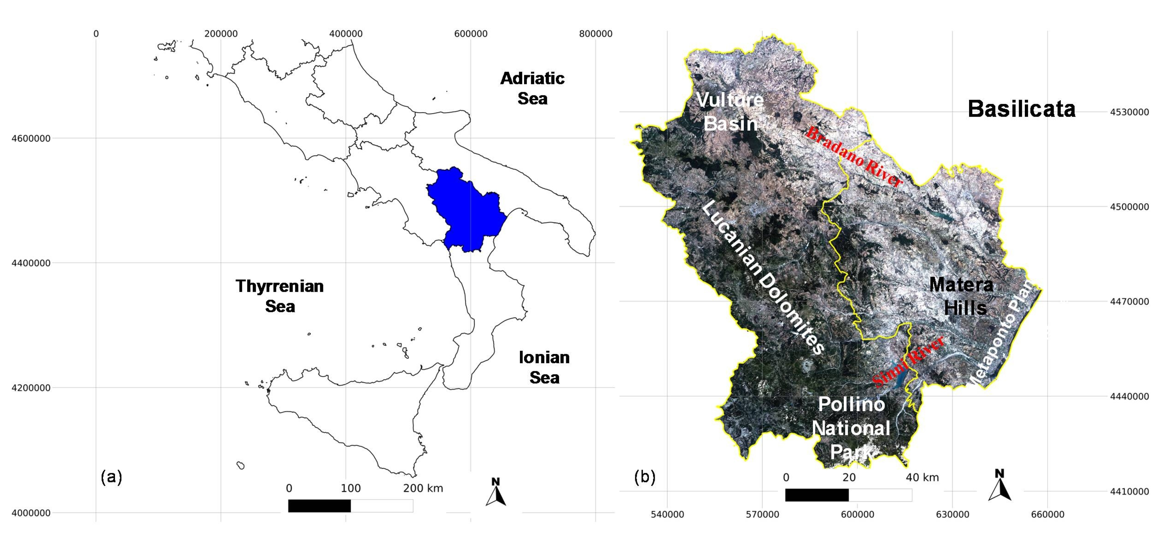
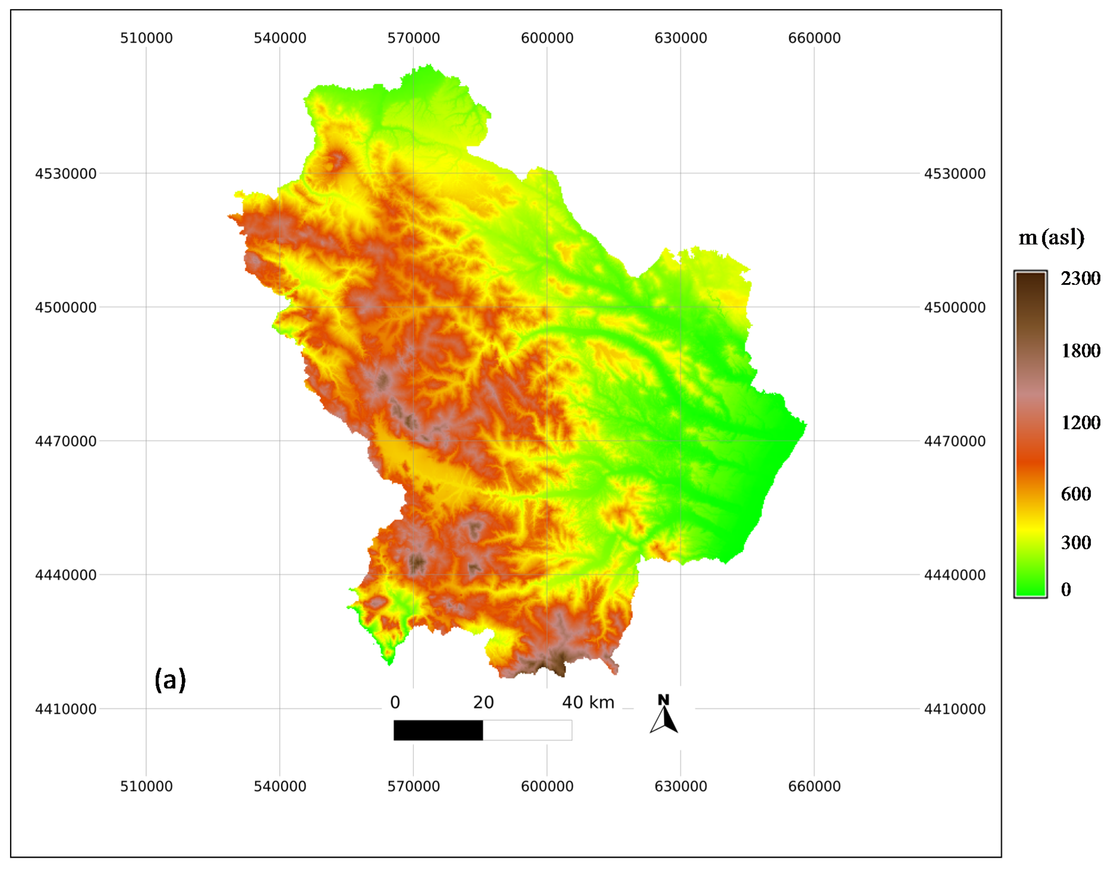
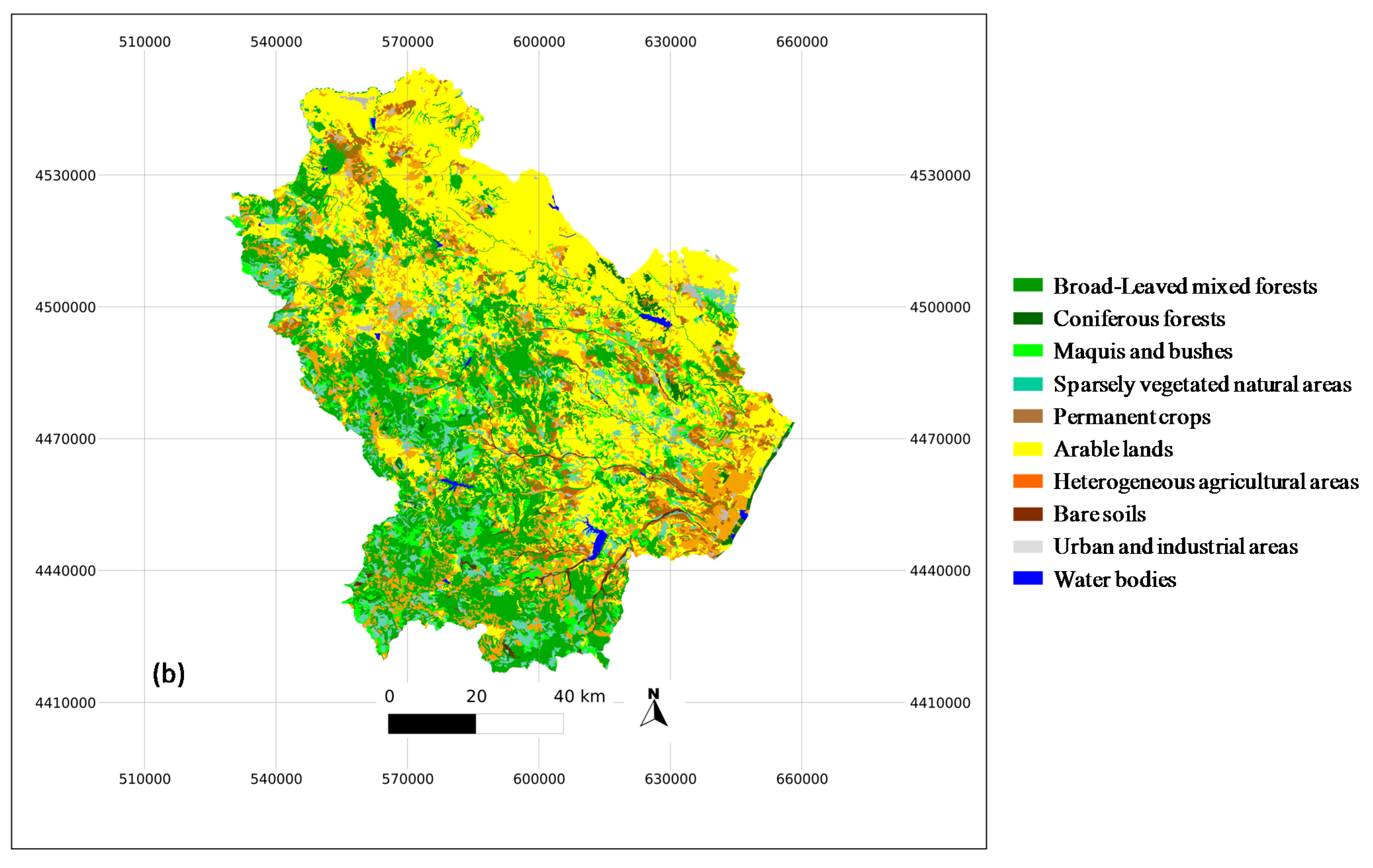
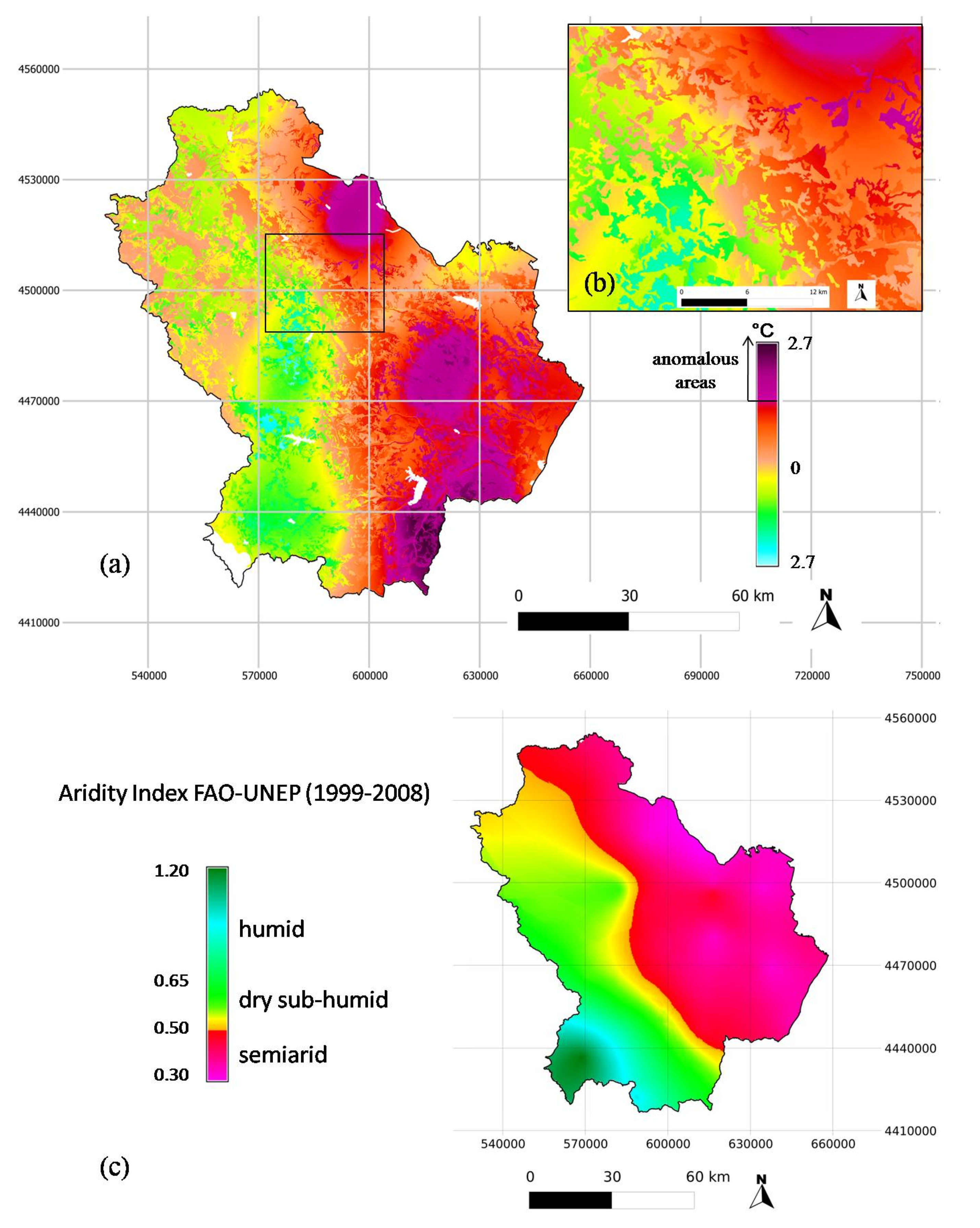
2. Study Area


3. Data
3.1. Landsat TM/ETM+ Data
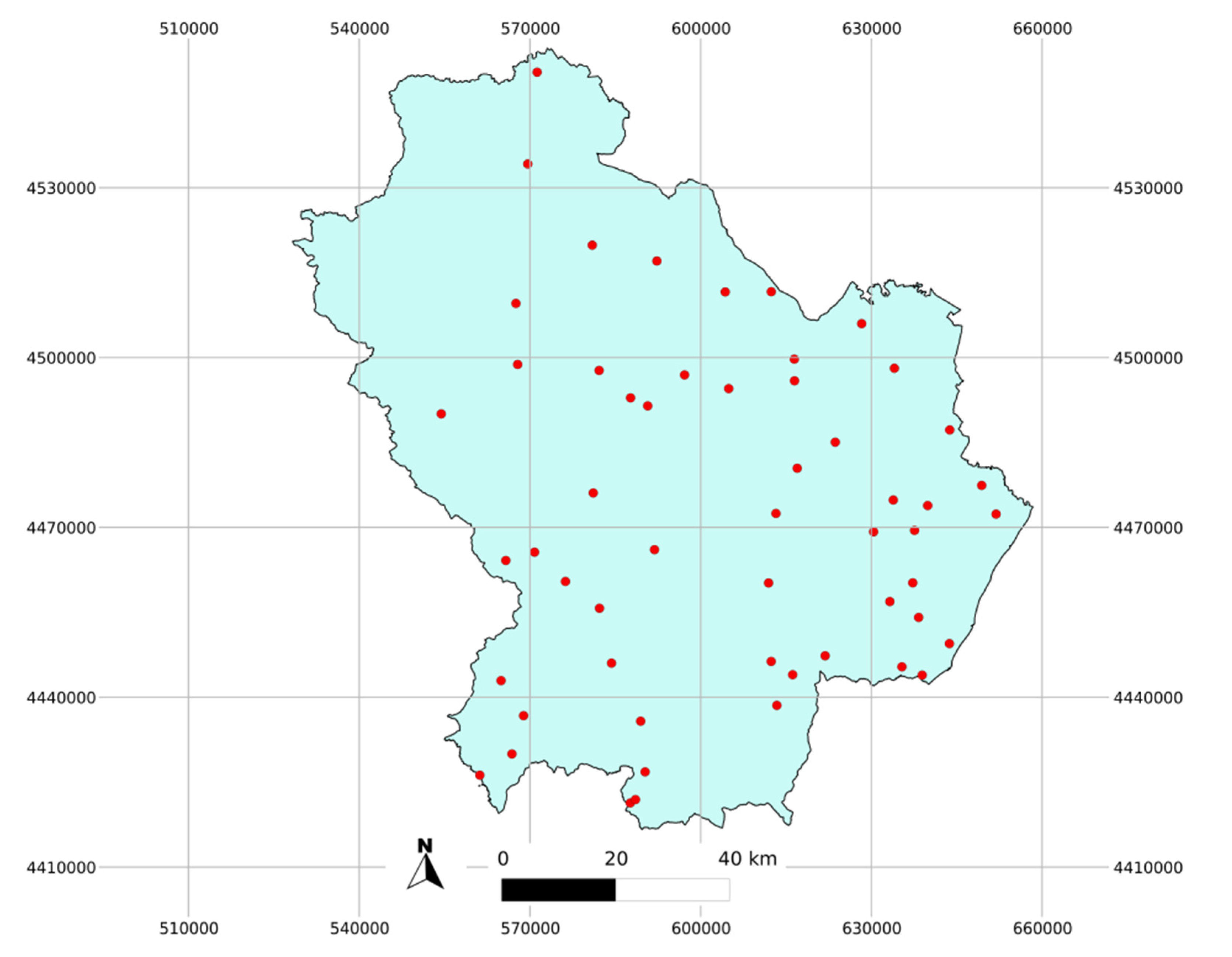
3.2. Meteorological Data

3.3. Elevation and Land Cover Maps
3.4. Auxiliary Data
4. Methods
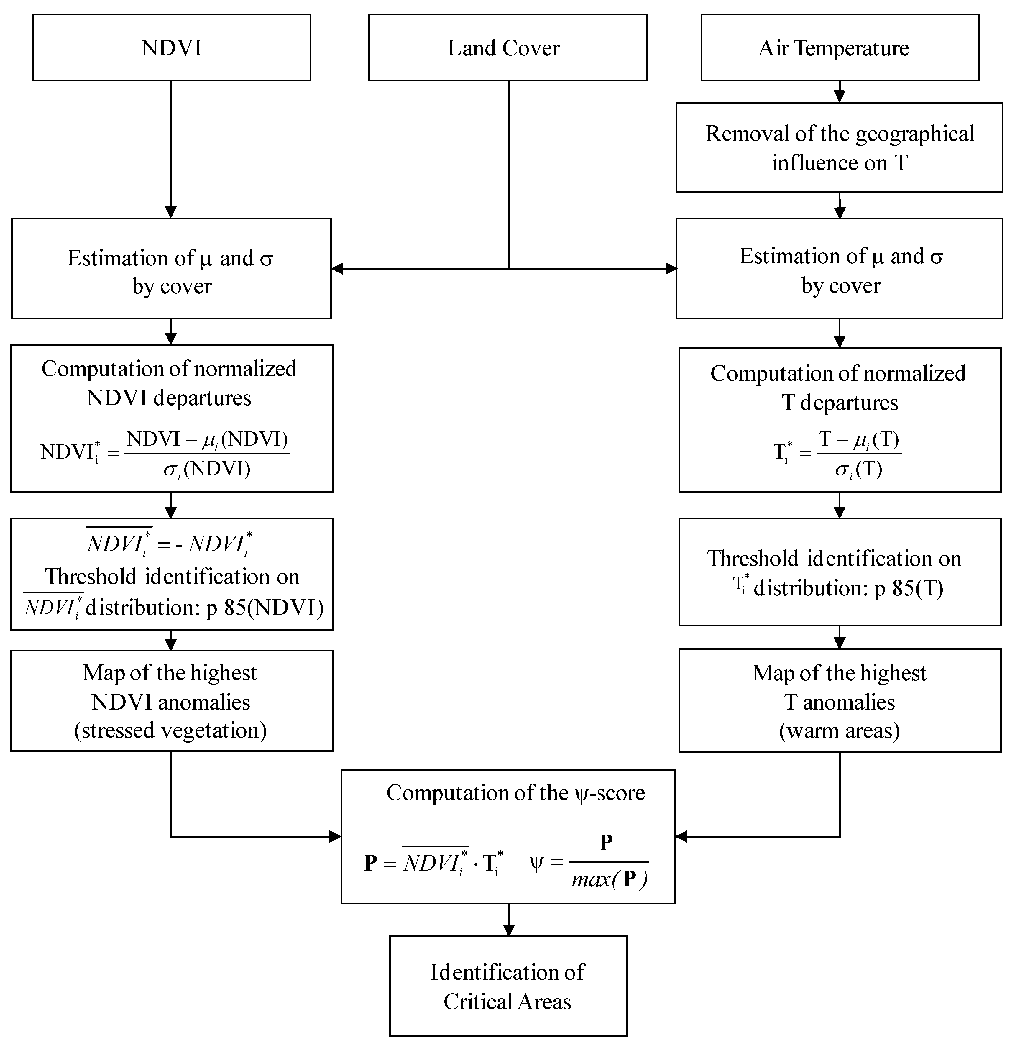
4.1. Spatialization of Air Temperature Records
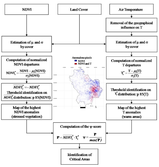
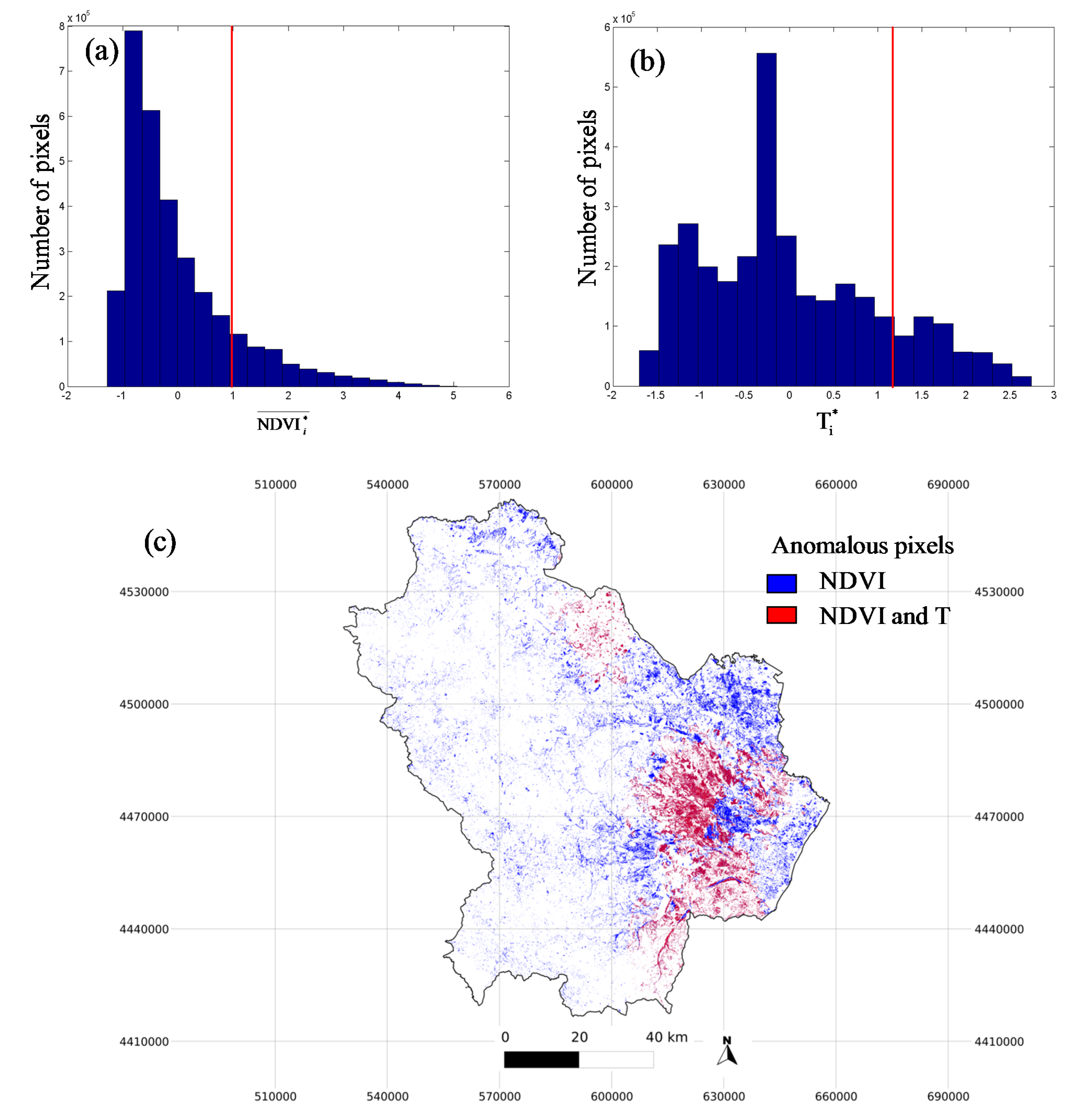
4.2. Identification of Critical Areas
4.2.1. Removal of Residual Non-Vegetated Effects
4.2.2. Statistical Procedure

5. Results and Discussion
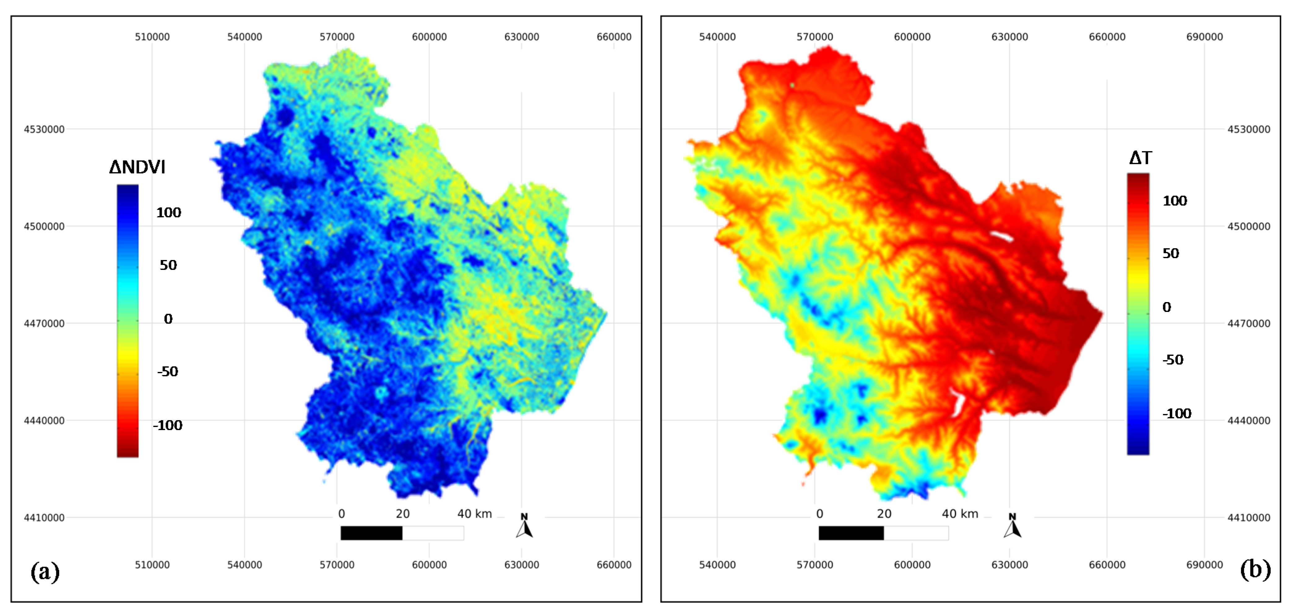
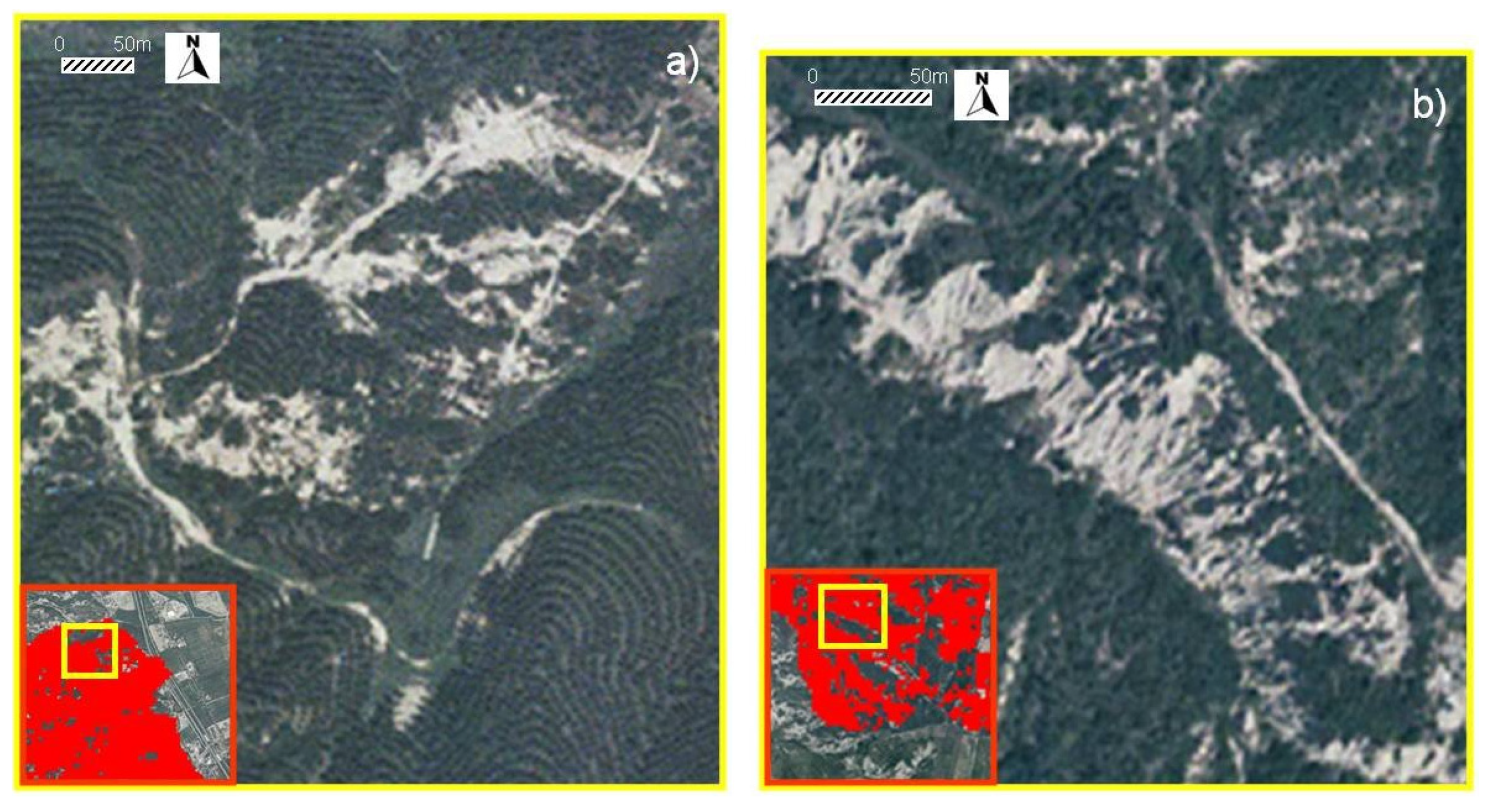
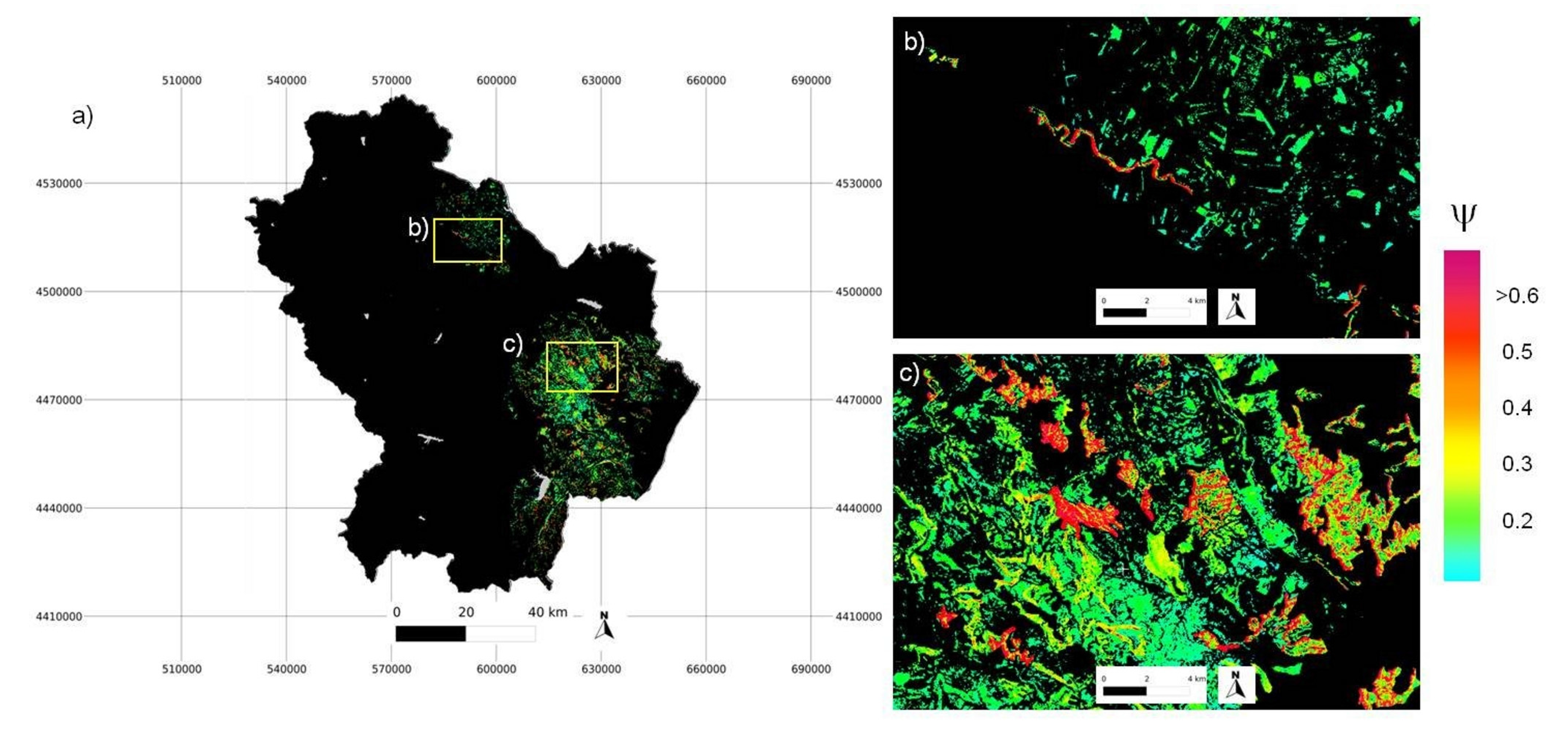
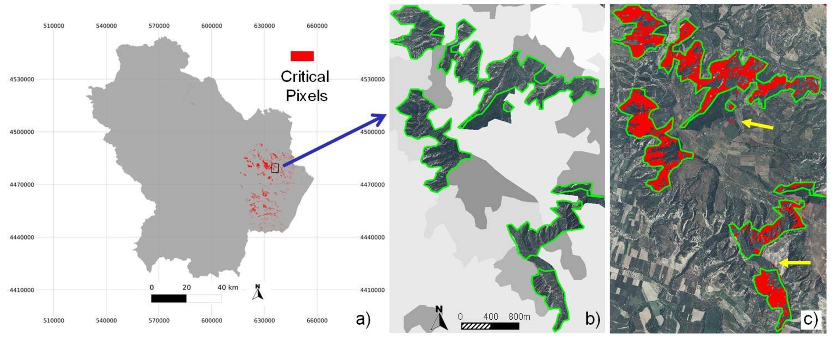
5.1. Critical Areas


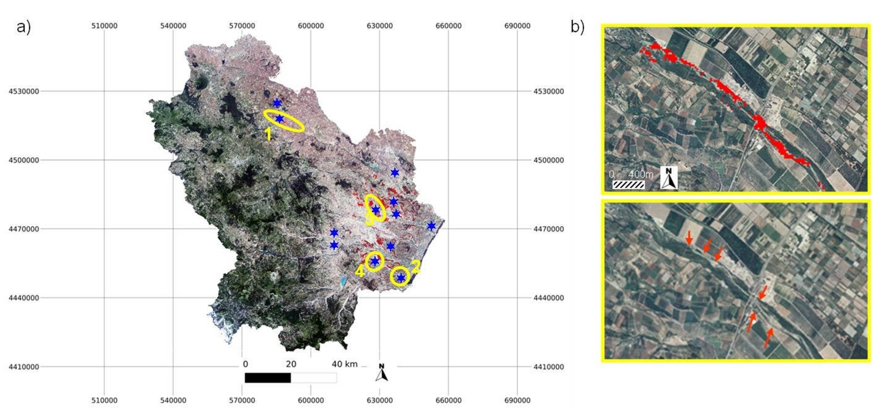
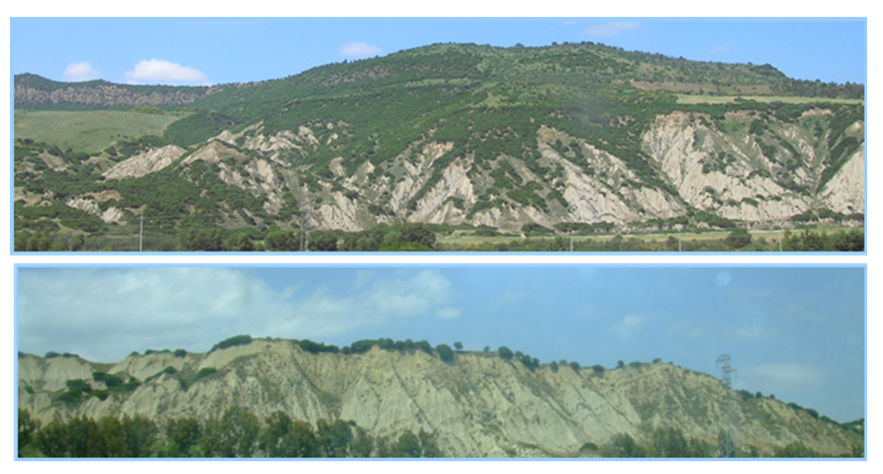
| Land Cover Classes | Percentage of Critical Pixels (%) |
|---|---|
| Broad-Leaved mixed forests | 88.6 |
| Maquis and bushes | 0.0 |
| Sparsely vegetated natural areas | 6.8 |
| Permanent crops | 0.2 |
| Arable lands | 0.1 |
| Heterogeneous agricultural areas | 3.7 |
| Bare soils | 0.3 |
5.2. Accuracy, Consistency, and Exportability
6. Conclusions
Acknowledgments
Author Contributions
Conflicts of Interest
References
- UNCCD Secretariat 2013. A Stronger UNCCD for a Land-Degradation Neutral World; Issue Brief; UNCCD: Bonn, Germany, 2013. [Google Scholar]
- UNEP 2011. UNEP Evaluation Office: Terminal Evaluation of the UNEP/FAO/GEF Project Land Degradation Assessment in Drylands (LADA). Available online: http://www.unep.org/eou/Portals/52/Reports/DL_LADA_TE_%20FinalReport.pdf (accessed on 12 January 2015).
- Adeel, Z.; Safriel, U.; Neimeijer, D.; White, R. Ecosystems and Human Well-Being: Desertification Synthesis; World Resources Institute: Washington, DC, USA, 2005. [Google Scholar]
- Romm, J. Desertification: The next dust bowl. Nature 2011, 478, 450–451. [Google Scholar] [CrossRef] [PubMed]
- Gibbs, H.K.; Salmon, J.M. Mapping the world’s degraded lands. Appl. Geogr. 2015, 57, 12–21. [Google Scholar] [CrossRef]
- Zdruli, P. Land resources of the mediterranean: Status, pressures, trends and impacts on future regional development. Land. Degrad. Dev. 2014, 25, 373–384. [Google Scholar] [CrossRef]
- Bajocco, S.; de Angelis, A.; Perini, L.; Ferrara, A.; Salvati, L. The impact of land use/land cover changes on land degradation dynamics: A Mediterranean case study. Environ. Manag. 2012, 49, 980–989. [Google Scholar] [CrossRef] [PubMed]
- Schaldach, R.; Wimmer, F.; Koch, J.; Volland, J.; Geißler, K.; Köchy, M. Model-based analysis of environmental impacts of grazing management in Eastern Mediterranean ecosystems in Jordan. J. Environ. Manag. 2013, 127, S84–S95. [Google Scholar] [CrossRef] [PubMed]
- Ibañez, J.; Valderrama, J.M.; Papanastasis, V.; Evangelou, C.; Puigdefabrigas, J. A multidisciplinary model for assessing degradation in Mediterranean rangelands. Land. Degrad. Dev. 2014, 25, 468–482. [Google Scholar] [CrossRef]
- Reynolds, J.F.; Smith, D.M.S.; Lambin, E.F.; Turner, B.L.; Mortimore, M.; Batterbury, S.P.J.; Downing, T.E.; Dowlatabadi, H.; Fernandez, R.J.; Herrick, J.E.; et al. Global desertification: Building a science for dryland development. Science 2007, 316, 847–851. [Google Scholar] [CrossRef] [PubMed]
- Carrara, P.; Bordogna, G.; Boschetti, M.; Brivio, P.A.; Nelson, A.; Stroppiana, D. A flexible multi-source spatial-data fusion system for environmental status assessment at continental scale. Int. J. Geogr. Inf. Sci. 2008, 22, 781–799. [Google Scholar] [CrossRef]
- Imbrenda, V.; D’Emilio, M.; Lanfredi, M.; Simoniello, T.; Ragosta, M.; Macchiato, M. Integrated indicators for the estimation of vulnerability to land degradation. In Soil Processes and Current Trendsin Quality Assessment; Hernandez Soriano, M.C., Ed.; Intech Open Access Publisher: Rijeka, Croatia, 2013; pp. 139–174. [Google Scholar]
- Kosmas, C.; Ferrara, A.; Briassouli, H.; Imeson, A. Methodology for mapping Environmentally Sensitive Areas (ESAs) to Desertification. The Medalus project: Mediterranean desertification and land use. In Manual on Key Indicators of Desertification and Mapping Environmentally Sensitive Areas to Desertification; Kosmas, C., Kirkby, M., Geeson, N., Eds.; EUR 18882, EU, DG XII: Brussels, Belgium, 1999; pp. 1–87. [Google Scholar]
- Imbrenda, V.; D’Emilio, M.; Lanfredi, M.; Macchiato, M.; Ragosta, M.; Simoniello, T. Indicators for the estimation of vulnerability to land degradation derived from soil compaction and vegetation cover. Eur. J. Soil Sci. 2014, 65, 907–923. [Google Scholar] [CrossRef]
- Eswaran, H.; Lal, R.; Reich, P.F. Land degradation: An overview. In Response to Land Degradation; Bridges, E.M., Hannam, I.D., Oldeman, L.R., Penning deVries, F.W.T., Scherr, S., Sombatpanit, S., Eds.; Oxford Press: New Delhi, India, 2001; pp. 20–35. [Google Scholar]
- Hill, J.; Stellmes, M.; Udelhoven, T.; Röder, A.; Sommer, S. Mediterranean desertification and land degradation. Mapping related land use change syndromes based on satellite observations. Glob. Planet. Chang. 2008, 64, 146–157. [Google Scholar] [CrossRef]
- Mueller, E.N.; Wainwright, J.; Parsons, A.J.; Turnbull, L.; Millington, J.D.A.; Papanastasis, V.P. Land degradation in drylands: Reevaluating pattern-process interrelationships and the role of ecogeomorphology. In Patterns of Land Degradation in Drylands: Understanding Self-Organised Ecogeomorphic Systems; Mueller, E.N., Wainwright, J., Parsons, A.J., Turnbull, L., Eds.; Springer Science+Business Media: Dordrecht, The Netherlands, 2014; Volume XI, pp. 367–383. [Google Scholar]
- Grainger, A. Is land degradation neutrality feasible in dry areas? J. Arid Environ. 2015, 112, 14–24. [Google Scholar] [CrossRef]
- Tal, A. The implications of environmental trading mechanisms on a future zero net land degradation protocol. J. Arid Environ. 2015, 112, 25–32. [Google Scholar] [CrossRef]
- Higginbottom, T.P.; Symeonakis, E. Assessing land degradation and desertification using vegetation index data: current frameworks and future directions. Remote Sens. 2014, 6, 9552–9575. [Google Scholar] [CrossRef]
- Bai, Z.G.; Dent, D.L.; Olsson, L.; Schaepman, M.E. Proxy global assessment of land degradation. Soil Use Manag. 2008, 24, 223–234. [Google Scholar] [CrossRef]
- Prince, S.D.; Becker-Reshef, I.; Rishmawi, K. Detection and mapping of long-term land degradation using local net production scaling: Application to Zimbabwe. Remote Sens. Environ. 2009, 113, 1046–1057. [Google Scholar] [CrossRef]
- Del Barrio, G.; Puigdefabregas, J.; Sanjuan, M.E.; Stellmes, M.; Ruiz, A. Assessment and monitoring of land condition in the Iberian Peninsula, 1989–2000. Remote Sens. Environ. 2010, 114, 1817–1832. [Google Scholar]
- Zhang, X.Y.; Goldberg, M.; Tarpley, D.; Friedl, M.A.; Morisette, J.; Kogan, F.; Yu, Y. Drought-induced vegetation stress in southwestern North America. Environ. Res. Lett. 2010, 5, 024008. [Google Scholar] [CrossRef]
- Tasumi, M.; Hirakawa, K.; Hasegawa, N.; Nishiwaki, A.; Kimura, R. Application of MODIS land products to assessment of land degradation of alpine rangeland in northern India with limited ground-based information. Remote Sens. 2014, 6, 9260–9276. [Google Scholar] [CrossRef]
- Eckert, S.; Hüsler, F.; Liniger, H.; Hodel, E. Trend analysis of MODIS NDVI time series for detecting land degradation and regeneration in Mongolia. J. Arid Environ. 2015, 113, 16–28. [Google Scholar] [CrossRef]
- Lanfredi, M.; Lasaponara, R.; Simoniello, T.; Cuomo, V.; Macchiato, M. Multi resolution spatial characterization of land degradation phenomena in Southern Italy from 1985 to 1999 using NOAA-AVHRR NDVI data. Geophys. Res. Lett. 2003, 30. [Google Scholar] [CrossRef]
- Hill, J.; Hostert, P.; Röder, A. Long-term observation of Mediterranean ecosystems with satellite remote sensing. In Recent Dynamics of the Mediterranean Vegetation and Landscape; Mazzoleni, S., di Pasquale, G., Mulligan, M., di Martino, P., Rego, F., Eds.; John Wiley & Sons Ltd.: Chichester, UK, 2004; pp. 33–43. [Google Scholar]
- Vicente-Serrano, S.M.; Cuadrat-Pratsc, J.M.; Romo, A. Aridity influence on vegetation patterns in the middle Ebro Valley (Spain): Evaluation by means of AVHRR images and climate interpolation techniques. J. Arid Environ. 2006, 66, 353–375. [Google Scholar] [CrossRef]
- Simoniello, T.; Lanfredi, M.; Liberti, M.; Coppola, R.; Macchiato, M. Estimation of vegetation cover resilience from satellite time series. Hydrol. Earth Syst. Sci. 2008, 12, 1053–1064. [Google Scholar] [CrossRef]
- Weissteiner, C.J.; Bottcher, K.; Sommer, S. Enhancing Remotely Sensed Low ResolutionVegetation Data for Assessing Mediterranean Areas Prone to Land Degradation. In Land Use and Land Cover Mapping in Europe: Practices &Trends; Manakos, I., Braun, M., Eds.; Springer Science+Business Media: Dordrecht, The Netherlands, 2014; pp. 341–362. [Google Scholar]
- Zhou, W.; Gang, C.; Zhou, F.; Li, J.; Dong, X.; Zhao, C. Quantitative assessment of the individual contribution of climate and human factors to desertification in northwest China using net primary productivity as an indicator. Ecol. Indic. 2015, 48, 560–569. [Google Scholar] [CrossRef]
- Stimson, H.C.; Breshears, D.D.; Ustin, S.L.; Kefauver, S.C. Spectral sensing of foliar water conditions in two co-occurring conifer species: Pinus edulis and Juniperus monosperma. Remote Sens. Environ. 2005, 96, 108–118. [Google Scholar] [CrossRef]
- Dutkiewicz, A.; Lewis, M.; Ostendorf, B. Evaluation and comparison of hyperspectral imagery for mapping surface symptoms of dryland salinity. Int. J. Remote Sens. 2009, 30, 693–719. [Google Scholar] [CrossRef]
- Röder, A.; Hill, J. Recent Advances in Remote Sensing and Geoinformation Processing for Land Degradation Assessment; ISPRS Book Series; Taylor and Francis Group: London, UK, 2009; p. 400. [Google Scholar]
- Santos, M.J.; Greenberg, J.A.; Ustin, S.L. Using hyperspectral remote sensing to detect and quantify southeastern pine senescence effects in red-cockaded woodpecker (Picoides borealis) habitat. Remote Sens. Environ. 2010, 114, 1242–1250. [Google Scholar] [CrossRef]
- Rossini, M.; Fava, F.; Cogliati, S.; Meroni, M.; Marchesi, A.; Panigada, C.; Giardino, C.; Busetto, L.; Migliavacca, M.; Amaducci, S.; et al. Assessing canopy PRI from airborne imagery to map water stress in maize. ISPRS J. Photogramm. Remote Sens. 2013, 86, 168–177. [Google Scholar] [CrossRef]
- Shrestha, D.P.; Margate, D.E.; van der Meer, F.; Anh, H.V. Analysis and classification of hyperspectral data for mapping land degradation, An application in southern Spain. Int. J. Appl. Earth Obs. Geoinf. 2005, 7, 85–96. [Google Scholar] [CrossRef]
- Lagacherie, P.; Baret, F.; Feret, J.B.; Madeira, J.; Robbez-Masson, J.M. Estimation of soil clay and calcium carbonate using laboratory, field and airborne hyperspectral measurements. Remote Sens. Environ. 2008, 112, 825–835. [Google Scholar] [CrossRef]
- Salas, C.; Ene, L.; Gregoire, T.G.; Næsset, E.; Gobakken, T. Modelling tree diameter from airborne laser scanning derived variables: A comparison of spatial statistical models. Remote Sens. Environ. 2010, 114, 1277–1285. [Google Scholar] [CrossRef]
- Garcia, M.; Riano, D.; Chuvieco, E.; Danson, F.M. Estimating biomass carbon stocks for a Mediterranean forest in central Spain using LiDAR height and intensity data. Remote Sens. Environ. 2010, 114, 816–830. [Google Scholar] [CrossRef]
- Ghosh, A.; Fassnacht, F.E.; Joshi, P.K.; Koch, B. A framework for mapping tree species combining hyperspectral and LiDAR data: Role of selected classifiers and sensor across three spatial scales. Int. J. Appl. Earth Obs. Geoinf. 2014, 26, 49–63. [Google Scholar] [CrossRef]
- Allan, J.L.; Darrell, W.G.; William, H.F. Using LiDAR data to map gullies and headwater streams under forest canopy: South Carolina, USA. Catena 2007, 71, 132–144. [Google Scholar]
- Cavalli, M.; Tarolli, P.; Marchi, L.; Dalla Fontana, G. The effectiveness of airborne LiDAR data in the recognition of channel-bed morphology. Catena 2008, 73, 249–260. [Google Scholar] [CrossRef]
- Jones, D.K.; Baker, M.E.; Miller, A.J.; Jarnagin, S.T.; Hogana, D.M. Tracking geomorphic signatures of watershed suburbanization with multi temporal LiDAR. Geomorphology 2014, 219, 42–52. [Google Scholar] [CrossRef]
- Metternicht, G.; Zinck, J.A.; Blanco, P.D.; del Valle, H.F. Remote sensing of land degradation: experiences from Latin America and the Caribbean. J. Environ. Qual. 2009, 39, 42–61. [Google Scholar] [CrossRef] [PubMed]
- Kaplan, S.; Blumberg, D.G.; Mamedov, E.; Orlovsky, L. Land-use change and land degradation in Turkmenistan in thepost-Soviet era. J. Arid Environ. 2014, 103, 96–106. [Google Scholar] [CrossRef]
- Vrieling, A.; de Jong, S.M.; Sterk, G.; Rodrigues, S.C. Timing of erosion and satellite data: A multi-resolution approach to soil erosion risk mapping. Int. J. Appl. Earth Obs. Geoinf. 2008, 10, 267–281. [Google Scholar] [CrossRef]
- Liberti, M.; Simoniello, T.; Carone, M.T.; Coppola, R.; D’Emilio, M.; Macchiato, M. Mapping badland areas using LANDSAT TM/ETM satellite imagery and morphological data. Geomorphology 2009, 106, 333–343. [Google Scholar] [CrossRef]
- Vågen, T.G.; Winowiecki, L.A.; Abegaz, A.; Hadgu, K.M. Landsat-based approaches for mapping of land degradation prevalence and soil functional properties in Ethiopia. Remote Sens. Environ. 2013, 134, 266–275. [Google Scholar] [CrossRef]
- Nawar, S.; Buddenbaum, H.; Hill, J.; Kozak, J. Modeling and mapping of soil salinity with reflectance spectroscopy and Landsat data using two quantitative methods (PLSR and MARS). Remote Sens. 2014, 6, 10813–10834. [Google Scholar] [CrossRef]
- Asner, G.P.; Knapp, D.E.; Broadbent, E.N.; Oliveira, P.J.C.; Keller, M.; Silva, J.N. Selective logging in the Brazilian Amazon. Science 2005, 5747, 480–482. [Google Scholar] [CrossRef] [PubMed]
- Matricardi, E.A.T.; Skole, D.L.; Pedlowski, M.A.; Chomentowski, W.; Fernandes, L.C. Assessment of tropical forest degradation by selective logging and fire using Landsat imagery. Remote Sens. Environ. 2010, 114, 1117–1129. [Google Scholar] [CrossRef]
- Dons, K.; Panduro, T.E.; Bhattarai, S.; Smith-Hall, C. Spatial patterns of subsistence extraction of forest products—Anindirect approach for estimation of forest degradation in dry forest. Appl. Geogr. 2014, 55, 292–299. [Google Scholar] [CrossRef]
- Röder, A.; Udelhoven, T.; Hill, J.; del Barrio, G.; Tsiourlis, G. Trend analysis of Landsat-TM and -ETM+ imagery to monitor grazing impact in a rangeland ecosystem in Northern Greece. Remote Sens. Environ. 2008, 112, 2863–2875. [Google Scholar] [CrossRef]
- Lanfredi, M.; Simoniello, T.; Macchiato, M. Temporal persistence in vegetation cover changes observed from satellite: Development of an estimation procedure in the test site of the Mediterranean Italy. Remote Sens. Environ. 2004, 93, 565–576. [Google Scholar] [CrossRef]
- Garcia, M.; Oyonarte, C.; Villagarcia, L.; Contreras, S.; Domingo, F.; Puigdefábregas, J. Monitoring land degradation risk using ASTER data: The non-evaporative fraction as an indicator of ecosystem function. Remote Sens. Environ. 2008, 112, 3720–3736. [Google Scholar] [CrossRef]
- Balling, R.C., Jr.; Klopatek, J.M.; Hilderbrandt, M.L.; Moritz, C.K.; Watts, C.J. Impacts of land degradation on historical temperature records from the Sonoran desert. Clim. Chang. 1998, 40, 669–681. [Google Scholar] [CrossRef]
- Arribas, A.; Gallardo, C.; Gaertner, M.A.; Castro, M. Sensitivity of the Iberian Peninsula climate to a land degradation. Clim. Dyn. 2003, 20, 477–489. [Google Scholar]
- Lu, H.; Liu, G. Recent observations of human-induced asymmetric effects on climate in very high-altitude area. PLoS ONE 2014, 9, e81535. [Google Scholar] [CrossRef] [PubMed]
- APAT-CNLSD. La Vulnerabilità Alla Desertificazione in Italia: Raccolta, Analisi, Confronto e Verifica Delle Procedure Cartografiche di Mappatura e Degli Indicatori a Scala Nazionale e Locale. Manuali e Linee Guida; (Collection and analysis of land degradation maps in Italy); CRA-UCEA: Rome, Italy, 2006; p. 128. [Google Scholar]
- Costantini, E.A.C.; Urbano, F.; Bonati, G.; Nino, P.; Fais, A. Atlante Nazionale Delle Aree a Rischio di Desertificazione; INEA: Roma, Italy, 2007; p. 108. [Google Scholar]
- EEA-European Environment Agency. The European Environment—State and Outlook; EEA-European Environment Agency: Copenhagen, Denmark, 2005. [Google Scholar]
- Piccarreta, M.; Capolongo, D.; Bonzi, F.; Bentivenga, M. Implications of decadal 840 changes in precipitation and land use policy to soil erosion in Basilicata, Italy. Catena 2006, 65, 138–161. [Google Scholar] [CrossRef]
- Sivakumar, M.K.V. Interactions between climate and desertification. Agric. For. Meteorol. 2007, 142, 143–155. [Google Scholar] [CrossRef]
- De Santis, F.; Giannossi, M.L.; Medici, L.; Summa, V.; Tateo, F. Impact of physico-chemical soil properties on erosion features in the Aliano area (Southern Italy). Catena 2010, 81, 172–181. [Google Scholar] [CrossRef]
- Greco, M.; Mirauda, D.; Squicciarino, G.; Telesca, V. Desertification risk assessment in southern Mediterranean areas. Adv. Geosci. 2005, 2, 243–247. [Google Scholar] [CrossRef]
- Bove, B.; Brindisi, P.; Ghisci, C.; Pacifico, G.; Summa, M.L. Indicatori climatici di desertificazione in Basilicata. Forest@ 2005, 2, 74–84. [Google Scholar]
- Chander, G.; Markham, B. Revised LANDSAT-5 TM radiometric calibration procedures and postcalibration dynamic ranges. IEEE Trans. Geosci. Remote Sens. 2003, 41, 2674–2677. [Google Scholar] [CrossRef]
- NASA-USGS. Landsat 7 Science Data Users Handbook. 2009. Available online: http://landsathandbook.gsfc.nasa.gov/pdfs/Landsat7_Handbook.pdf (accessed on 12 January 2015). [Google Scholar]
- Simoniello, T.; Carone, M.T.; Grippa, A.; Liberti, M.; Coppola, R.; Macchiato, M. Inter-calibration of Landsat-TM/ETM scenes in heterogeneous areas. Geophys. Res. Abstr. 2008, 10. SRef-ID:1607-7962/gra/EGU2008-A-11986. [Google Scholar]
- Kaufman, Y.J.; Wald, A.; Remer, L.A.; Gao, B.; Li, R.; Flynn, L. The MODIS 2.1 μm channel-Correlation with visible reflectance for use in remote sensing of aerosol. IEEE Trans. Geosci. Remote Sens. 1997, 35, 1–13. [Google Scholar] [CrossRef]
- Coppola, R.; Liberti, M.; D’Emilio, M.; Lanfredi, M.; Simoniello, T.; Macchiato, M. Combined approach for air temperature spatialization using DEM, latitude and sea distance: Variability of monthly data in Southern Italy. In Proceedings of the Workshop Spatial Data Methods for Environmental and Ecological Processes, Foggia, Italy, 14–15 September 2006.
- Lanfredi, M.; Coppola, R.; D’Emilio, M.; Imbrenda, V.; Macchiato, M.; Simoniello, T. A geostatistics-assisted approach to the deterministic approximation of climate data. Environ. Model. Softw. 2015, 66, 69–77. [Google Scholar] [CrossRef]
- Cressie, N. Spatial prediction and ordinary kriging. Math. Geol. 1988, 20, 405–421. [Google Scholar] [CrossRef]
- Schoonover, J.E.; Williard, K.W.J.; Zaczek, J.J.; Mangun, J.C.; Carver, A.D. Nutrient attenuation in agricultural surface runoff by riparian buffer zones in Southern Illinois, USA. Agrofor. Syst. 2005, 64, 169–180. [Google Scholar] [CrossRef]
- Carone, M.T.; Simoniello, T.; Manfreda, S.; Caricato, G. Watershed influence on fluvial ecosystems: An integrated methodology for river water quality management. Environ. Monit. Assess. 2009, 152, 327–342. [Google Scholar] [CrossRef] [PubMed]
- Basilicata Region. Forest Plan 2006–2008; Regione Basilicata: Potenza, Italy, 2006. [Google Scholar]
- Basilicata Region. Reforestation Plan 2009–2011; Regione Basilicata: Potenza, Italy, 2009. [Google Scholar]
- Basilicata Region. Ten Year Program of Forestation 2013–2022; Regione Basilicata: Potenza, Italy, 2013. [Google Scholar]
- Summa, V.; Tateo, F.; Medici, L.; Giannossi, L. The role of mineralogy, geochemistry and grain size in badland development in Pisticci (Basilicata, Southern Italy). Earth Surf. Process. Landf. 2007, 32, 980–997. [Google Scholar] [CrossRef]
- Simoniello, T.; Coluzzi, R.; Imbrenda, V.; Lanfredi, M. Land cover changes and forest landscape evolution (1985–2009) in a typical Mediterranean agroforestry system (high Agri Valley). Nat. Hazards Earth Syst. Sci. 2015, 15, 1201–1214. [Google Scholar] [CrossRef]
- Drusch, M.; del Bello, U.; Carlier, S.; Colin, O.; Fernandez, V.; Gascon, F.; Hoersch, B.; Isola, C.; Laberinto, P.; Martimort, P.; et al. Sentinel-2: ESA’s optical high-resolution mission for GMES operational services. Remote Sens. Environ. 2012, 120, 25–36. [Google Scholar] [CrossRef]
© 2015 by the authors; licensee MDPI, Basel, Switzerland. This article is an open access article distributed under the terms and conditions of the Creative Commons Attribution license (http://creativecommons.org/licenses/by/4.0/).
Share and Cite
Lanfredi, M.; Coppola, R.; Simoniello, T.; Coluzzi, R.; D'Emilio, M.; Imbrenda, V.; Macchiato, M. Early Identification of Land Degradation Hotspots in Complex Bio-Geographic Regions. Remote Sens. 2015, 7, 8154-8179. https://doi.org/10.3390/rs70608154
Lanfredi M, Coppola R, Simoniello T, Coluzzi R, D'Emilio M, Imbrenda V, Macchiato M. Early Identification of Land Degradation Hotspots in Complex Bio-Geographic Regions. Remote Sensing. 2015; 7(6):8154-8179. https://doi.org/10.3390/rs70608154
Chicago/Turabian StyleLanfredi, Maria, Rosa Coppola, Tiziana Simoniello, Rosa Coluzzi, Mariagrazia D'Emilio, Vito Imbrenda, and Maria Macchiato. 2015. "Early Identification of Land Degradation Hotspots in Complex Bio-Geographic Regions" Remote Sensing 7, no. 6: 8154-8179. https://doi.org/10.3390/rs70608154