Potential of C and X Band SAR for Shrub Growth Monitoring in Sub-Arctic Environments

Abstract

The Arctic and sub-Arctic environments have seen a rapid growth of shrub vegetation at the expense of the Arctic tundra in recent decades. In order to develop better tools to assess and understand this phenomenon, the sensitivity of multi-polarized SAR backscattering at C and X band to shrub density and height is studied under various conditions. RADARSAT-2 and TerraSAR-X images were acquired from November 2011 to March 2012 over the Umiujaq community in northern Quebec (56.55°N, 76.55°W) and compared to in situ measurements of shrub vegetation density and height collected during the summer of 2009. The results show that σ⁰ is sensitive to changes in shrub coverage up to 20% and is sensitive to changes in shrub height up to around 1 m. The cross-polarized backscattering $\left({\sigma }_{{}^{HV}}^0\right)$ displays the best sensitivity to both shrub height and density, and RADARSAT-2 is more sensitive to shrub height, as TerraSAR-X tends to saturate more rapidly with increasing volume scattering from the shrub branches. These results demonstrate that SAR data could provide essential information, not only on the spatial expansion of shrub vegetation, but also on its vertical growth, especially at early stages of colonization.

1. Introduction

The Arctic and sub-Arctic environments are undergoing rapid and dramatic changes due to the rise in air temperatures, which has been observed in the past few decades. This rise affects many aspects of the sub-Arctic ecosystem, from the thawing of permafrost to the changes in vegetation cover and their combined effect on the local populations, as well as on fauna and floristic diversity. One of the consequences of the warming Arctic climate that has received some attention is the expansion of the shrub vegetation at the expense of the Arctic tundra [1–4]. Studies suggest that the presence of shrubs can trigger a feedback loop, where windblown snow is captured by shrub branches, favouring snow accumulation, which leads to warmer ground temperatures during the winter and accelerated onset of growth in the spring [2,5,6]. This can also have an effect on the permafrost thawing processes, since ground temperatures will remain relatively warm during the winter. Most investigations in this field [7–12] have used time series of in situ measurements often combined with aerial photography and satellite imagery in the visible to infrared spectrum to assess these changes. These methods have proven useful, but suffer from some limitations: in situ measurements do not provide a good spatial coverage and can prove very costly in remote areas; aerial photography and satellite imagery in the visible to infrared spectrum cannot provide information on the vertical structure of the vegetation. Satellite-mounted Synthetic Aperture Radar (SAR), being an active sensor with wavelengths ranging from millimetres to metres, has the capacity to penetrate the vegetation canopy and to provide information on the vertical structure of the vegetation, as well as the underlying ground. Information on the vertical structure is important, since it can have a direct impact on snow accumulation.

While there have been many studies on the effects of natural vegetation on SAR backscattering coefficients, most of them were conducted over forested areas and were aimed at characterizing structural elements from trees, such as trunks and canopies [13–21]. Since the impact of shrubs in forested areas can be minor on SAR backscattering, the measurement of their characteristics has been largely ignored. There have been a few investigations that have focused their efforts on shrub vegetation, but they were mostly conducted in arid or semi-arid areas [22–25]. This research is part of the Permafrost and Climate Change in Northern Coastal Canada project funded by ArcticNet, which aims to analyse how permafrost responds to changing climate. The local variations in permafrost thawing patterns are affected by many environmental factors, such as the spatial distribution of snow accumulation and vegetation cover. While snow acts as an insulator during the winter, shrub vegetation provides shade in the summer, resulting in cooler ground temperatures throughout the season. Therefore, the development of snow mass and shrub vegetation mapping methods would help to understand the spatial variations in permafrost behaviour. The mapping of snow mass using SAR data has been attempted in the area [26,27] and revealed the importance of shrub vegetation on SAR backscattering, even during the winter season. To enable the retrieval of snow characteristics in these types of environments, it is therefore essential to have a better understanding of the effects of shrub vegetation on SAR backscattering. This paper will study the sensitivity of polarimetric and multi-frequency SAR data to sub-Arctic shrub vegetation characteristics, more specifically height and ground coverage. Of particular interest is the seasonal changes occurring in the transition from fall to winter as the ground and vegetation freeze and snow covers the shrubs. No study in the open literature has addressed this issue up to now.

2. Materials and Methods

2.1. Study Area and In Situ Measurements

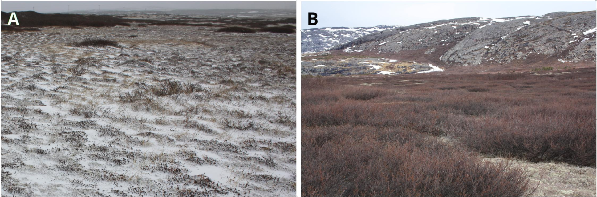
The study area is a 60-km² region situated in the vicinity of the Inuit community of Umiujaq (56.55°N, 76.55°W) on the eastern shore of the Hudson Bay, Nunavik (northern Quebec, Canada; see Figure 1). It is a discontinuous permafrost zone positioned at the northern tree line, forming a transition between the forest tundra to the south and the shrub tundra to the north. The geomorphology of the area is characterized by a cuesta formation sloping gently eastward from Hudson Bay for nearly 5 km, up to an altitude of 330 metres, at which point it forms steep, mainly east-facing cliffs. At the foot of these cliffs, we find Tasiapik Valley to the north and the Guillaume-Delisle Lake to the southeast. The vegetation cover in the coastal region is made up of various coastal tundra plant communities (graminoids, forbs, prostrate dwarf shrubs, lichen and moss) with a few patches of erect shrubs, mostly of dwarf birch (Betula glandulosa Michx.) and willow species (Salix argyrocarpa Andersson, S. glauca L. var. cordifolia (Pursh) Dorn, S. planifolia Pursh, S. vestita Pursh). Scattered black spruce (Picea mariana (Mill.) BSP) krummholz can also be found. Tasiapik Valley is mainly erect shrub tundra dominated by dwarf birch mixed with a few willows (mainly Salix planifolia, Labrador tea (Rhododendron groenlandicum (Oeder) Kron and Judd) and green alder (Alnus viridis (Chaix) DC. subsp. crispa (Ait.) Turrill). Prostrate dwarf shrub-lichen tundra is found on lithalsa summits and at higher valley-side elevations. Clusters of black spruce are found in the lowermost areas of the valley. The dominant soil type in the area is exposed bedrock with thin and discontinuous alteration deposits, found at higher altitudes on the cuesta formation and on elevated plateaus further inland. At lower altitudes, the soil types differ between the coastal and Tasiapik Valley areas; the former is predominantly covered by sand deposits, while the latter is predominantly covered by silt and clay with a thin organic layer. Small wetlands and thermokarst ponds are also scattered in the Tasiapik Valley. Figure 1 shows a topographic map of the area with the positioning of the shrub sampling plots, and Figure 2 shows pictures taken in May 2010 depicting the types of environments found in the study area.

In situ measurements of vegetation characteristics were collected during the summer of 2009 to validate the results of aerial photography analysis and to assess temporal changes in shrub vegetation characteristics [28]. A total of 238 circular plots with a 10-metre diameter was sampled. Each species of shrub and tree was identified; the percentage of the ground that they covered within the plot was measured, as well as up to three main heights for each species when their cover was distinctly unequal due to varying topography and exposure within a given plot. The type of soil, its moisture conditions and the topographic position were also documented. The vegetation height and coverage measurements were classified into 8 classes, which are detailed in

Table 1. Classes used for sampling vegetation height (m) and vegetation coverage (%) during field measurements.

Classes	0	1	2	3	4	5	6	7
Height (m)	0	0–0.25	0.25–0.50	0.50–1	1–1.5	1.5–2.5	2.5–5	>5
Coverage (%)	0	0–5	5–15	15–25	25–50	50–75	75–90	90–100

. Note that the height and percent coverage intervals of the classes are not equally distributed.

Snow sampling campaigns were coordinated with the RADARSAT-2 and TerraSAR-X satellite data acquisitions. Snow depth, density and snow water equivalent (SWE) were measured using a Standard Metric 3600 Federal Snow Sampling Tube for 65 (March) and 87 (April) sites covering various terrain types. The positioning of sampling sites were chosen so that they would match vegetation surveys made in 2009 in order to compare snow accumulation and characteristics with shrub vegetation structure. Snowpits were dug at selected locations to gather information from the different layers of the snowpack on particle size and shape in addition to snow densities.

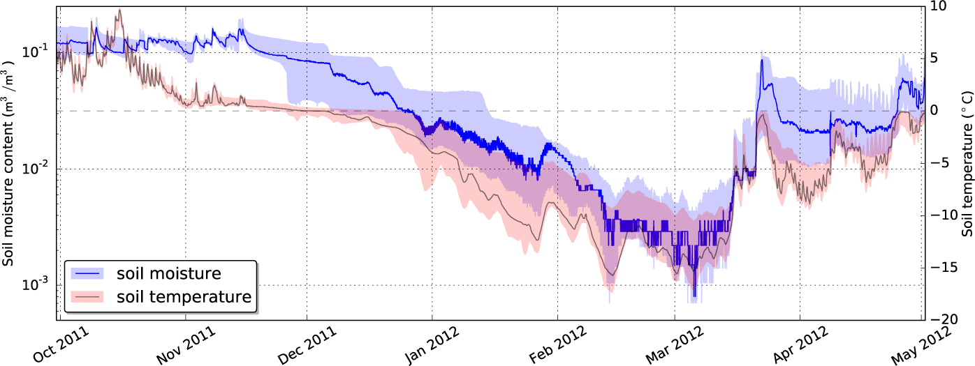
Ground temperatures and soil moisture content were also measured between August 2011 and August 2012. This was done using HOBO^® 12-bit Temperature Smart Sensors and HOBO^® Soil Moisture Smart Sensors coupled to a micro station. A total of 9 sites were chosen for the soil moisture and temperature measurements, four of which were in the coastal area and the other five in the valley area. The soil moisture measurements were taken at three different depths, 5 cm, 10 cm and 15 cm, and the temperature was taken at a depth of 5 cm. The sites were chosen in order to be as representative as possible of each type of environment. In the coastal area, two sites were set up on an elevated plateau with little shrub vegetation, and the two others were set up at lower altitudes in areas with some shrub vegetation. In the valley area, three sites were set up in the southern part, at lower altitudes, in areas with dense shrub coverage and higher soil moisture, while the two other sites were set up in the northern part at a higher altitude with scattered shrub coverage and dryer soils. Unfortunately, not all data loggers were retrieved after 12 months due to equipment failure at two sites in the coastal area, but the two sites were in different areas, so it was still possible to capture the environmental variability.

2.2. Satellite and GIS Datasets

A series of RADARSAT-2 single-look complex (SLC) fine quad-pol (FQ) scenes (HH, HV, VH, VV polarization) were acquired over the study area between October 2011 and April 2012. Dual-polarized TerraSAR-X single-look slant range complex (SSC) strip map (SM) scenes (HH, HV polarization) were also acquired over the area between November 2011 and April 2012. RADARSAT-2 operates at C band with a frequency of 5.4 GHz; the nominal resolution for the FQ beam is 5.2 m × 7.6 m (slant range × azimuth). TerraSAR-X operates at X band with a frequency of 9.65 GHz; the nominal resolution for the dual-pol SM mode is 5.2 m × 6.6 m (slant range × azimuth). All of the acquisitions were made on descending orbits with two incidence angle modes, one at low incidence with θ ≈ 27° and one at high incidence with θ ≈ 38°. The choices for the orbit and incidence modes were made in order to maximize the coverage of the study area with both sensors while capturing a good range of incidence angles.

Table 2. Acquisition dates and characteristics of SAR images.

Date	Sensor	Polarizations	Incidence Angle (θ)
12 November 2011	RADARSAT-2	quad-pol	38°
13 November 2011	TerraSAR-X	HH + HV	27°
15 November 2011	RADARSAT-2	quad-pol	27°
19 November 2011	TerraSAR-X	HH + HV	38°
05 December 2011	TerraSAR-X	HH + HV	27°
06 December 2011	RADARSAT-2	quad-pol	38°
09 December 2011	RADARSAT-2	quad-pol	27°
11 March 2012	RADARSAT-2	quad-pol	38°
13 March 2012	TerraSAR-X	HH + HV	27°
14 March 2012	RADARSAT-2	quad-pol	27°
19 March 2012	TerraSAR-X	HH + HV	38°

shows the acquisition date and parameters for each scene.

An SRTM digital elevation model (DEM) of the area combined with a high resolution Lidar DEM (1-metre horizontal resolution) were used to perform terrain corrections of the SAR images. A high-resolution Geoeye-1 multispectral image (1.65-metre resolution) was also used to complement the visual interpretation of the SAR imagery.

The single-look complex images were processed using the PolSARpro software ( https://earth.esa.int/web/polsarpro), and the 2 × 2 complex scattering matrices [S] from each image were converted to covariance matrices 〈[C]〉, which, for RADARSAT-2, take the form [29]:

$$\langle [C]\rangle =\left[\begin{array}{ccc}\langle {\left|S_{HH}\right|}^2\rangle & \sqrt{2}\langle S_{HH}{S}_{HV}^{*}\rangle & \langle S_{HH}{S}_{VV}^{*}\rangle \\ \sqrt{2}\langle S_{HV}{S}_{HH}^{*}\rangle & 2\langle {\left|S_{HV}\right|}^2\rangle & \sqrt{2}\langle S_{HV}{S}_{VV}^{*}\rangle \\ \langle S_{VV}{S}_{HH}^{*}\rangle & \sqrt{2}\langle S_{VV}{S}_{HH}^{*}\rangle & \langle {\left|S_{VV}\right|}^2\rangle \end{array}\right]$$

(1)

where 〈〉 denotes the ensemble averaging and S_pq are the individual elements of the scattering matrix [S] with q the transmitting polarization and p receiving polarization. Since RADARSAT-2 is a monostatic sensor, the reciprocity theorem applies, and S_HV = S_VH, resulting in a 3 × 3 covariance matrix. For the TerraSAR-X data, only dual-polarized images were available, so the covariance matrix takes the form:

$$\langle [C]\rangle =\left[\begin{array}{cc}\langle {\left|S_{HH}\right|}^2\rangle & \sqrt{2}\langle S_{HH}{S}_{HV}^{*}\rangle \\ \sqrt{2}\langle S_{HV}{S}_{HH}^{*}\rangle & 2\langle {\left|S_{HV}\right|}^2\rangle \end{array}\right]$$

(2)

The diagonal elements of the covariance matrices are used as the backscattering coefficients in the different polarization channels $\left(C={\sigma }_{HH}^0,C_{22}={\sigma }_{HV}^0,C_{33}={\sigma }_{VV}^0\right)$; the relationship between S_pq and ${\sigma }_{{}^{pq}}^0$is [29]:

$${\sigma }_{{}^{pq}}^0=\frac{4\pi }{A}\langle {|S_{pq}|}^2\rangle$$

(3)

where A represents the area on the ground of the corresponding resolution cell. This normalization is done during the production of the covariance matrix by applying a lookup table provided with the SLC image. Averages are provided through multi-looking, which is performed in two steps for the current study. The first step achieves a 2 look multi-looking by averaging the values of 2 pixels in the azimuth direction of the SAR image during the original extraction of the covariance matrix. The second step is achieved during the speckle filtering process during which the improved sigma speckle filter [30] was used with a 5 × 5 pixel window. The total number of looks then amounts to 50 before the geo-corrections.

Once the covariance matrices were extracted and the speckle filter applied, the images were geo-corrected using the MapReady software from the Alaska Satellite Facility ( https://www.asf.alaska.edu/data-tools/mapready). The orthorectification method generates a simulated SAR image, using a combination of orbit and look angle parameters of the sensor with a DEM, and then performs a coregistration of the acquired SAR image with the simulated SAR image. The combination of a high-resolution (1 m) LiDAR-based DEM and the presence of steep topographic features in the area provided good pixel localization accuracy. There was one corner reflector installed on the bedrock north of the village, which provided the only known stable ground control point in the area. The RADARSAT-2 images were also resampled to a 9-metre ground resolution, and the TerraSAR-X images were resampled to 6 metres; these correspond roughly to the average pixel sizes of the SLC images. The pixel localization accuracy was on the order of 0.5 pixels on average (≈ 4 to 5 metres) for RADARSAT-2 and on the order of 1 pixel on average (≈ 6 metres) for TerraSAR-X. This was found to be sufficient for the current analysis given the positioning accuracy of the vegetation sampling sites, which were recorded using a standard GPS. The RADARSAT-2 images were also resampled to a 9-metre ground resolution, and the TerraSAR-X images were resampled to 6 metres; these correspond roughly to the average pixel sizes of the SLC images. To compare SAR backscattering to the shrub characteristics, the σ⁰ values used were taken from the pixels corresponding to the centre of the vegetation sampling plots.

2.3. Shrub Vegetation and SAR Interactions

Sub-Arctic terrains at the ecotone between the forest tundra and the shrub tundra exhibit high spatial heterogeneity in their vegetation cover and ground properties. This gives rise to a complex mixture of scattering mechanisms composed of direct scattering from the ground attenuated by the vegetation, volume scattering from the crown of the shrubs and interaction terms between the ground and the crown. In the presence of trees and boulders, there are also ground-trunk and ground-rock double-bounce mechanisms appearing. As the temperature drops during the fall, the soil and vegetation freeze, and the leaves fall from deciduous shrubs, reducing the dielectric coefficients and overall backscattering, as well as the attenuation.

When snow covers the shrubs during the winter, new scattering mechanisms appear: volume scattering from the snow, snow-ground interaction terms, snow-branch volume interaction terms, as well as some surface scattering from the snow surface [18]. There is also attenuation of ground scattering due to loss within the snow layer through volume scattering and some absorption, while the incidence angle at the snow-ground interface is modified due to refraction within the snowpack. The dielectric contrast between shrub branches and snow is inferior to the one between branches and air, which will slightly reduce the volume scattering from the branches. The effect of snow is dependent on many parameters, especially its moisture content, as well as the frequency of the sensor [29,31–33]. In the present case, snow conditions were always dry at the time of SAR data acquisitions, so wet snow will not be considered. At the C band, the volume scattering and attenuation from dry snow are very low and often ignored due to their minor effect compared to soil and vegetation backscattering [18]. It was also demonstrated that, at incidence angles lower than 35°, scattering from the ground remains dominant in the presence of snow [34]. At the X band, the effect of snow is more important due to the grain size being larger relative to the wavelength [32,33,35]. Figure 3 shows the major scattering mechanisms that can be found within this type of environment.

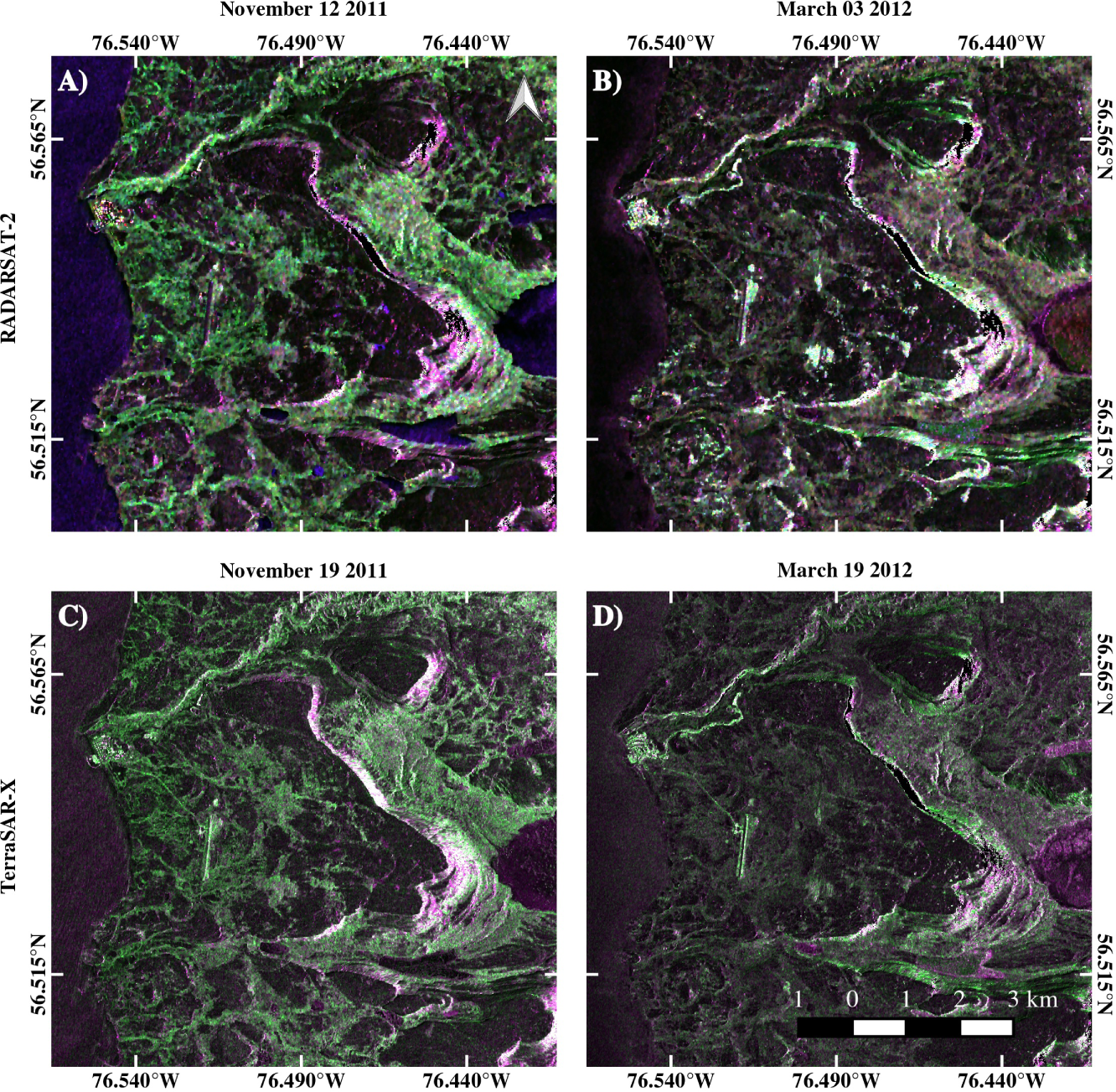
In order to assess the sensitivity of SAR backscattering to shrub characteristics, the σ⁰ values from RADARSAT-2 and TerraSAR-X were sampled over the vegetation survey sites for all dates, incidence angles and polarizations and then compared to shrub density and height. The first analysis focuses on the response of σ⁰ at C and X bands to the percentage of shrub coverage within each plot to estimate the potential of SAR data to map the spatial expansion of shrubs. The second analysis focuses on the response of σ⁰ to shrub height in order to see if it is possible to estimate the vertical growth of shrub vegetation. To have a better understanding of the variations in the observed backscattering coefficients, we also look at the effect of the soil moisture regime and snow depths on σ⁰ values. Figure 4 shows RGB colour composites of RADARSAT-2 and TerraSAR-X images where $\text{red}={\sigma }_{HH}^0$, $\text{green}={\sigma }_{HV}^0$ and $\text{blue}={\sigma }_{VV}^0$ for RADARSAT-2 and ${\sigma }_{HH}^0$ for TerraSAR-X. The green areas correspond to vegetation; shrub vegetation induces depolarization on the backscattered signal, generating cross-polarized backscattering.

3. Results and Discussion

3.1. Backscattering Coefficient Sensitivity to Shrub Density

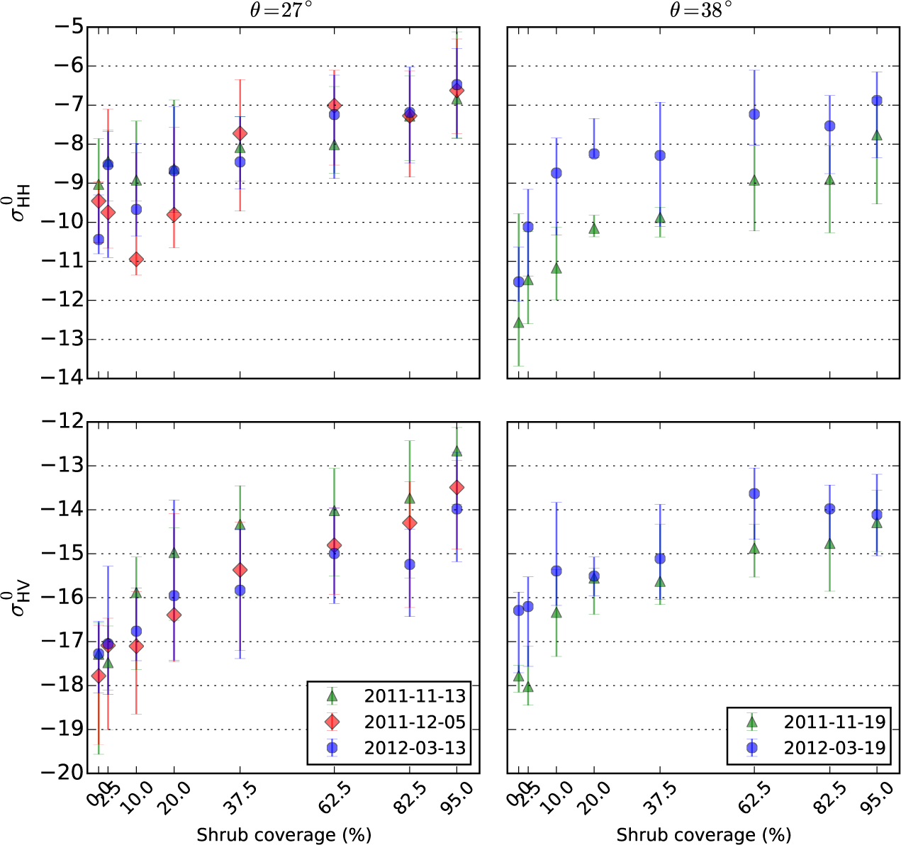
Backscattering coefficients show a tendency to increase with shrub density at C band (Figure 5). The slope of this relationship is generally steeper at lower shrub coverage ranging between 0% and 20%. For areas with shrub coverage above 20%, the sensitivity of σ⁰ to shrub density declines. This decline combined with the high variability in backscattering coefficients indicates that other shrub components, such as height, branch size and structure, come into play at higher densities. The incidence angle affects the magnitude of the backscattering, as well as the sensitivity to shrub density. The backscattering at θ = 27° incidence is consistently higher than at θ = 38° by around 1 dB to 2 dB, but the latter is more sensitive to shrub coverage, which is consistent with scattering theory [29], since higher incidence angles lead to higher sensitivity to volume scattering relative to surface scattering. Cross-polarized backscattering also displays a higher dynamic range than co-polarized backscattering, since it is generated by the depolarization processes generally associated with vegetation scattering.

The temporal analysis of the C band backscattering coefficients shows that overall σ⁰ tends to decrease throughout the acquisition period spanning from November–March, while the sensitivity to change in shrub coverage remains appreciable. However, this sensitivity is not constant, and the changes depend on polarization and incidence angle. The increase in average σ⁰ in relation to shrub density is greater in December for co-polarized backscattering, while the cross-polarized backscattering displays higher sensitivity in November. In general, co-polarized backscattering is more affected by surface scattering from the ground, especially at C band, so the higher sensitivity to shrub density observed in December could be linked to the frozen state of the ground, which leads to higher relative sensitivity to volume scattering from shrub branches. The fact that the increase is more pronounced at higher incidence (θ = 38°) strengthens this hypothesis. As for the cross-polarized backscattering, at both incidence angles, the increase is greater in November, before the ground freeze-up. Since cross-polarized backscattering is affected by the depolarizing effect of the shrub branches, the higher dielectric constants of the branches before the freeze-up generates stronger ${\sigma }_{HV}^0$ and a greater sensitivity to shrub density. In December, once the ground and shrub branches are frozen, the sensitivity to shrub density drops, but the effect is more discernible at θ = 38° for which the average increase in ${\sigma }_{HV}^0$ in relation to shrub density is 9.3 dB in November and only 6.3 dB in December, while it goes from 8.5 dB down to 8.3 dB for the same period at θ = 38°. There is then little change from December–March at θ = 27°, but at θ = 38°, the average increase of ${\sigma }_{HV}^0$ drops from 8.3 dB down to 5.7 dB for that period. A Student’s t-test shows that there is no statistical difference between the means in December compared to those in March for the 0%, 2.5% and 10% coverage classes, so the perceived difference in sensitivity to shrub coverage in that range is not significant. The reduced total backscattering observed in March is most likely related to the lower ground temperatures (Figure 6), which causes the ground’s dielectric constant to drop and yields lower backscattering coefficients.

The backscattering coefficients in the X band dataset are generally stronger than C band, and the sensitivity to shrub density (Figure 7) for analogous incidence angles and polarizations is weaker. This indicates that X band backscattering tends to saturate more rapidly at higher shrub densities. The total increase in mean backscattering coefficients in relation to shrub density ranges between 2.5 dB and 3.8 dB for ${\sigma }_{HH}^0$ and between 2.7 dB and 5.0 dB for ${\sigma }_{HV}^0$. When doing a temporal comparison (Student’s t-test), there are no significant differences between the mean ${\sigma }_{HH}^0$ values at θ = 27°, and for ${\sigma }_{HV}^0$, only the sites with shrub coverage ≥62.5% (mean of cover Class 5: 50%–75%) display significant differences in their means. At θ = 38°, however, the temporal change is significant, and contrary to C band, there is an increase in backscattering coefficients between the fall and winter season. This is coherent with the theory in [29], since X band, with its shorter wavelength than C band, is more sensitive to scattering from smaller particles, such as snow grains, consequently increasing the volume scattering generated by the snowpack.

3.2. Backscattering Coefficient Sensitivity to Shrub Height

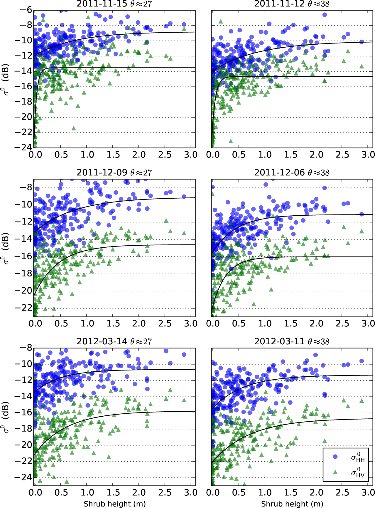
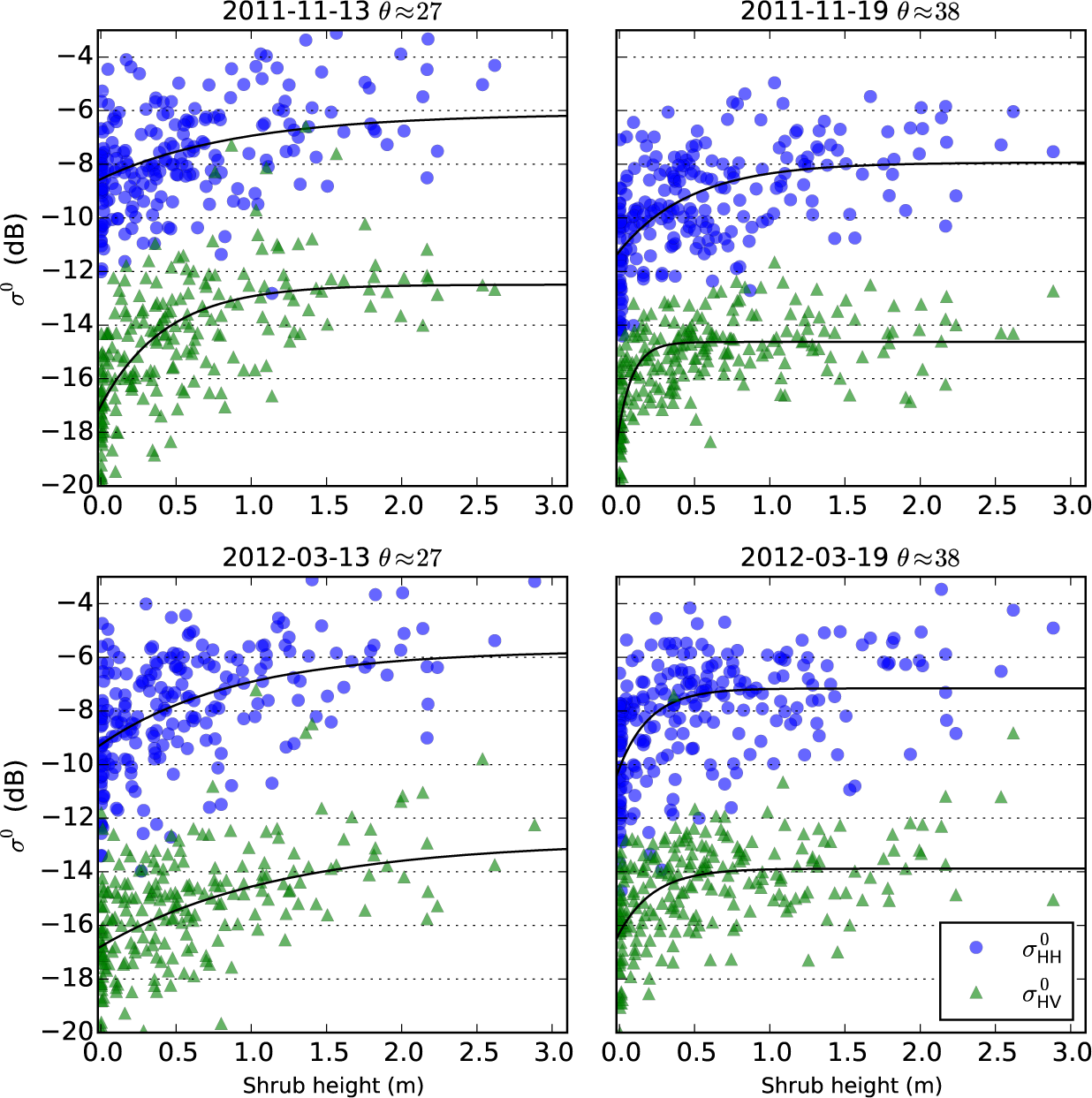
In order to evaluate the sensitivity of the backscattering coefficients to shrub height, the height of each plant species within the sampling plots was weighted with the percent coverage that the species occupies within the plots to obtain a weighted average of the vegetation height (h_w). This weighted average was then compared to the backscattering coefficients in the different polarizations. Since the weighting process also takes into account the shrub-free areas, a large proportion of sites can have low h_w, even if some stands observed on the site can be relatively tall. Figures 8 and 9 show examples of σ⁰ values from November 2011, December 2011 and March 2012 images plotted against h_w. It can be observed that the majority of the data is concentrated below the one metre mark, and further analysis showed that the sites covered with less than 20% of shrubs are concentrated below 0.25 metres. The relationship between σ⁰ and h_w has a similar aspect to the one between σ⁰ and the Leaf Area Index (LAI) of certain types of agricultural crops observed by Ulaby et al. [29]. It was then decided to use the model proposed by Ulaby et al. for the relationship between σ⁰ and shrub height. The model used to fit the data takes the form:

$${\sigma }_{fpq\theta }^0(h)=A_1(1-e^{-h/b})+A_2{e}^{-h/b}$$

(4)

where ${\sigma }_{fpq\theta }^0$ is the backscattering coefficient (in dB) at frequency f, polarization pq and incidence angle θ and h is the weighted mean of shrub height. A₁, A₂ and b are constants that vary with frequency, incidence and polarization. A₁ is related to the σ⁰ level at which the signal saturates and where shrub vegetation height does not exert any significant influence; A₂ is the intercept and is related to the effect of ground backscattering on the total σ⁰, and b is related to the range of vegetation height for which we can observe significant variations in σ⁰; the actual range is ≈ 3b.

The model was tested for all of the acquisition dates, incidence angles and polarization states. Results for RADARSAT-2 can be viewed in

Table 3. Results for regression analysis of RADARSAT-2 backscattering coefficients as a function of shrub mean height.

Date	Incidence	Polarization	A1 (dB)	A2 (dB)	b (m)	R2	RMSE	${\mathrm{\Delta }}_{A_1{A}_2}(\mathrm{dB})$	3b (m)
15 November 2011	27	HH	−8.8	−11.9	0.78	0.23	1.82	3.1	2.33
		HV	−13.5	−20.7	0.05	0.48	2.53	7.2	0.16
		VV	−9.4	−12.0	0.65	0.20	1.74	2.6	1.94
09 December 2011	27	HH	−9.1	−13.1	0.78	0.30	1.97	4.0	2.35
		HV	−14.6	−20.3	0.46	0.47	2.13	5.7	1.39
		VV	−9.6	−13.2	0.62	0.27	1.97	3.6	1.87
14 March 2012	27	HH	−10.6	−13.4	0.50	0.19	2.04	2.8	1.50
		HV	−15.8	−21.1	0.62	0.35	2.46	5.3	1.87
		VV	−10.9	−13.6	0.49	0.18	1.97	2.6	1.48
12 November 2011	38	HH	−10.0	−14.0	0.88	0.37	1.60	3.9	2.63
		HV	−14.7	−21.6	0.07	0.58	2.05	7.0	0.20
		VV	−10.0	−13.9	0.73	0.39	1.58	3.9	2.18
06 December 2011	38	HH	−11.1	−15.6	0.45	0.44	1.77	4.4	1.35
		HV	−16.0	−21.9	0.26	0.46	2.35	5.9	0.79
		VV	−11.6	−15.6	0.50	0.38	1.74	3.9	1.49
11 March 2012	38	HH	−11.3	−15.5	0.60	0.33	1.99	4.1	1.79
		HV	−16.6	−22.1	0.72	0.35	2.40	5.4	2.17
		VV	−12.0	−15.6	0.64	0.27	1.95	3.6	1.93

, and those for TerraSAR-X can be viewed in

Table 4. Results for regression analysis of TerraSAR-X backscattering coefficients as a function of shrub mean height.

Date	Incidence	Polarization	A1 (dB)	A2 (dB)	b (m)	R2	RMSE	${\mathrm{\Delta }}_{A_1{A}_2}(\mathrm{dB})$	3b (m)
2011 November 13	27	HH	−6.1	−8.6	0.92	0.12	1.97	2.4	2.77
		HV	−12.5	−17.0	0.43	0.42	1.87	4.5	1.29
2011 December 05	27	HH	−6.3	−9.5	0.43	0.23	2.04	3.2	1.30
		HV	−13.3	−17.3	0.53	0.38	1.75	4.0	1.58
2012 March 13	27	HH	−5.7	−9.3	0.92	0.16	2.42	3.5	2.75
		HV	−12.9	−16.8	1.19	0.17	2.40	3.9	3.57
2011 November 19	38	HH	−7.9	−11.2	0.48	0.33	1.66	3.3	1.44
		HV	−14.6	−17.8	0.10	0.46	1.20	3.1	0.29
2012 March 19	38	HH	−7.2	−10.1	0.21	0.22	2.03	3.0	0.62
		HV	−13.9	−16.3	0.23	0.23	1.61	2.4	0.69

. Backscattering sensitivity to shrub height can be characterized by two parameters extracted from the model: the average dynamic range in σ⁰ calculated from the difference between A₁ and $A_2({\mathrm{\Delta }}_{A_1{A}_2})$ and the effective range in vegetation height approximated by 3b. As with the shrub coverage analysis, ${\sigma }_{HV}^0$ at C band tends to exhibit a greater dynamic range, especially during the late fall. In November and December, ${\mathrm{\Delta }}_{A_1{A}_2}$ varies from 5.7 dB to 7.2 dB for cross-polarized backscattering, while ${\mathrm{\Delta }}_{A_1{A}_2}$ varies from 2.6 dB–4.4 dB for co-polarized backscattering. However, the effective range for ${\sigma }_{HV}^0$ is relatively low, and the values of 3b vary between 0.16 m and 1.39 m for the same dates, while the values for ${\sigma }_{HH}^0$ and ${\sigma }_{VV}^0$ vary between 1.35 m and 2.63m. In all cases, the p-values of the A₁, A₂ parameters were well below 0.001. The p-values for the b parameter were below 0.05; the highest values found are for co-polarized backscattering coefficients at 27° incidence and for ${\sigma }_{VV}^0$ at 38° on March 11 and range between 0.0013 and 0.0106. The agreement with the model is better with cross-polarized backscattering, and R² values range between 0.46 and 0.58 in November and December, while R² for co-polarized backscattering range between 0.20 and 0.44 for the same dates. Again, this result was expected, as cross-polarized backscattering is most affected by volume scattering from the shrub branches.

During the winter, in the presence of snow, the agreement with the model tends to drop for all polarizations and incidence angles, but the effect on ${\mathrm{\Delta }}_{A_1{A}_2}$ and effective range has a variable behaviour depending on polarization and incidence angle. At HV polarization, ${\mathrm{\Delta }}_{A_1{A}_2}$ constantly decreases from November–March, while the effective range constantly increases. For co-polarized backscattering, the temporal changes depend on incidence angles. At lower incidence, ${\mathrm{\Delta }}_{A_1{A}_2}$ increases from November–December by around 1 dB, while the effective range remains relatively constant, but in March, both ${\mathrm{\Delta }}_{A_1{A}_2}$ and 3b values decrease significantly. At higher incidence, the changes in ${\mathrm{\Delta }}_{A_1{A}_2}$ are less than 1 dB for the period, while 3b decreases between November and December and then slightly increases in March. It should however be noted that the agreement with the model constantly decreases from November–March, so the observed variations are less significant.

Looking at Figures 8 and 9, and in particular at the RMSE values of the model, it can be seen that the March ${\sigma }_{HV}^0$ displays a wide dispersion, especially for values at lower shrub heights. The lower sensitivity and correlation with shrub height in March can be explained in part by the presence of snow. Snow generates some attenuation and volume scattering, which can produce noise when evaluating shrub height, but it also reduces the dielectric contrast between the shrub branches and their surrounding medium. The effective permittivity of dry snow (ε_s), which is mostly dependent on snow density [36], is slightly greater than air, in the order of ε_s=1.5, but combined with the reduced permittivity of the vegetation [18,37] during the winter can contribute in reducing the sensitivity of SAR to shrub height. The temporal variations of co-polarized backscattering coefficients are different from the cross-polarized one: the December datasets have the most sensitivity to shrub height, while the sensitivities and correlations are lower in November. This dissimilarity can be explained by the surface scattering from the ground, which is stronger in November, before the ground freeze-up, compared to December, when the ground is mostly frozen. Since co-polarized backscattering is more sensitive to surface scattering mechanisms than cross-polarized backscattering, the correlation between co-polarized coefficients and vegetation height tends to drop in the presence of stronger surface scattering relative to volume scattering. In March, however, the observed drop in correlation and sensitivity to shrub height is due to different mechanisms. During that period, the ground is completely frozen, and its temperature is lower than in December, further reducing the surface scattering component, so the drop in sensitivity to shrub height could be due to the presence of snow. Field data show that higher shrubs will often retain more snow, creating a deeper snowpack in areas where shrubs are taller and more dense. For example, sites with h_w > 0.5 m accumulated on average 61.7 cm of snow during the winter of 2012, while sites with h_w ≤ 0.5 m accumulated an average of 28.3 cm and sites with h_w ≤ 0.25 m accumulated an average of 19.1 cm. However, vegetation is not the only determining factor influencing snow depth, as local topography and the local wind direction and wind velocity also play a major role in the snow accumulation process.

The TerraSAR-X backscattering coefficients have relatively weaker correlations with shrub height (0.12 ≤ R² ≤ 0.46) and display slightly lower dynamic ranges $(2.4dB\le {\mathrm{\Delta }}_{A_1{A}_2}\le 4.5dB)$ than what is observed at C band. The p-values of the A₁ and A₂ parameters were all well below 0.001. The p-values for the b parameter were slightly higher than at C band, but were all below 0.05, except for ${\sigma }_{HH}^0$ at 27° on 13 November, which was 0.089. The highest p-values were found in March for the co- and cross-polarized backscattering at both incidence angles and for ${\sigma }_{HH}^0$ at 27° on 5 December, and they ranged between 0.0027 and 0.0439. There are also less temporal variations in dynamic ranges $({\mathrm{\Delta }}_{A_1{A}_2})$, which are relatively constant between acquisitions. One of the major difference between X and C band, however, is the effect of incidence angle on the sensitivity to shrub height, especially at HH polarization. At higher incidence (θ ≈ 38°), the agreement with the model is slightly better and the RMSE is lower. This can be explained by the relative increase of the importance of volume scattering with increasing incidence angle, reducing the relative importance of surface scattering. Since X band provides less penetration through the canopy, the surface scattering mechanism is less important than at C band, and the lower sensitivity and correlation in November and December at X band are most likely due to a saturation of the volume scattering from the branches. Given our primary objectives and the complexity of the terrain, ground roughness measurements were not performed in the area, so it is difficult to estimate the contribution of the ground surface on the backscattered signal, but it is possible to gain insight into the importance of this mechanism by looking at the changes in soil moisture and temperature. Looking at the temporal changes in σ⁰ values compared to ground moisture and temperature, there is little change between November and December backscattering coefficients at θ ≈ 27°, only a slight decrease in sensitivity and correlation at HV polarization and an increase of the sensitivity and correlation to vegetation height at HH polarization. The increased sensitivity and correlation observed with the co-polarized backscattering in December could be explained by the relative reduction in ground scattering due to the freeze-up of the ground. The other important difference between RADARSAT-2 and TerraSAR-X data is that, while ${\mathrm{\Delta }}_{A_1{A}_2}$ remains similar between fall and winter at X band, the values of A₁ and A₂ rise in March, contrary to what is observed at C band. This effect is linked to the presence of snow in March, which increases the volume scattering component of the total backscattered power. The shorter wavelength at X band results in increased scattering from the snow grains, which are larger relative to the wavelength. These results show that the effect of shrub vegetation on SAR backscattering is quite important and needs to be considered in studies using SAR data in sub-Arctic environments. It is especially important to projects aiming at measuring snow characteristics using X band SAR, such as the one proposed by Rott et al. [38,39]. While some corrections were added to the model in order to take into account the effect of vegetation [40,41], it was mainly forest vegetation that was considered, and shrub vegetation was not mentioned in the study.

3.3. Sources of the Observed Variability

The analysis of the radar backscattering response to shrub density and height reveals a significant sensitivity of σ⁰ values to those vegetation parameters that vary as a function of incidence angle, polarization, frequency and the timing of the acquisitions. There is however a high variance in the backscattering coefficients regardless of the different configurations, and RMSE values for the model analysis are around 2 dB on average for RADARSAT-2 and 1.8 dB for TerraSAR-X. There are many factors that can explain this high variability, which is related either to the nature of the data used or to environmental characteristics. One important source of error is linked to the treatment that was performed on in situ shrub vegetation measurements to convert them to weighted average height. Due to the fact that vegetation height and ground coverage were recorded as classes with irregular intervals, the conversion to average height using the median point of those intervals could introduce estimation errors. Moreover, these errors are greater for classes of taller vegetation due to their wider intervals. Once again, these measurements were optimal for the needs of the original survey due to the highly complex structure of the vegetation in the area and the fact that the initial objective was not to gather data for SAR estimation of vegetation height.

In such a complex environment, many components affect the scattering properties of a given target, and there are many environmental factors that can explain the observed variability. Another vegetation characteristic that was not considered for the current analysis is the vertical structure of the various species found in the study area. The model proposed by Ulaby [29] was developed for agricultural applications, and different versions of the model were used depending on the species studied. In the current case, the heterogeneous nature of the environment results in the presence of multiple species of shrubs within a single resolution cell, which can produce uncertainty in the model fitting. Scattering from the ground surface is another major component of the total backscattered power in this case, especially with RADARSAT-2. The full assessment of the ground scattering component is not possible due to the complexity of the terrain and the lack of measurements related to ground properties. There is however some information on soil temperature and moisture content at a few sites (not necessarily at the same location as the vegetation sampling sites), which can give better insight into the temporal behaviour of the backscattering. As explained above, the drop in temperature in December leads to ground freeze-up, reducing the ground’s dielectric constant and the relative importance of ground surface scattering compared to volume scattering from shrub vegetation. The slight increase in sensitivity to shrub height in December, after the ground freeze-up, compared to November is a consequence of this phenomenon. Consequently, the spatial variations of soil properties and moisture regime will also create fluctuations in the backscattering coefficients and can explain part of the observed variability. Shrub species, soil types and soil moisture regime are generally interconnected and form distinct ecosystems. In order to provide better modelling results, a spatial segmentation and classification of the territory could be performed to take into account the physical characteristics of these ecosystems. Further studies will therefore focus on classification of SAR images.

4. Conclusions

This study looked at the effect of shrub vegetation on backscattering coefficients measured with RADARSAT-2 and TerraSAR-X. In situ measurements of shrub height and ground coverage were compared to measured σ⁰ values at various incidence angles, polarizations and frequencies to evaluate their sensitivity to those two shrub characteristics. It has been shown that the backscattering coefficients are sensitive to shrub coverage up to a density of 20%, at which point, the sensitivity tends to drop significantly. The sensitivity of backscattering coefficients to shrub height was also assessed. Results show that the backscattering coefficients have the highest sensitivity (≈7 dB) and the highest correlation (0.48 ≤ R² ≤ 0.58) to shrub height at C band at HV polarization, which is consistent with existing literature for crop height [29]. The HV polarization is more affected by the random scattering generated by the branches within the shrub canopy, and the shorter wavelength of the X band provides less penetration, resulting in lower sensitivity (maximum of 4.5 dB) and correlations (R² ≤ 0.46). The sensitivity to shrub vegetation remains significant during the winter, when dry snow covers the shrubs; however, it was found that the response is different between X band and C band. At C band, the backscattering is generally lower during the winter (≈ 2 dB–4 dB), and the sensitivity and correlation with shrub height are weaker; while at X band, the backscattering coefficients are higher during the winter (≈ 0.5 dB–1 dB), but the correlations and sensitivity stay relatively weak throughout the year with little variation. It was also observed that soil moisture and temperature play a significant role in the backscattering coefficients at C band, even in the presence of shrub vegetation and snow, which shows that ground scattering remains a major component of the total backscattered power at this frequency. The effect of soil characteristics was not as obvious at X band, and the presence of snow during the winter increased the total backscattered power, which indicates that volume scattering from vegetation and snow tends to dominate at this frequency.

The findings exposed in this paper provide a good basis to further improvements in the assessment of shrub growth and expansion in Arctic and sub-Arctic regions. The data show that SAR backscattering is very sensitive to shrub height when the stands are shorter than one metre. It is therefore expected that the initial stages of shrub growth in the Arctic tundra can be detected from space-borne SAR sensors. This would provide an important tool to assess and monitor the ongoing shrubification phenomenon observed at these latitudes, while improving carbon budget estimations and predictions of permafrost thaw caused by snow-vegetation interactions. Further research will focus on the latter subject in order to estimate snow mass accumulations within shrub vegetation using SAR data.

References

- Sturm, M.; Racine, C.; Tape, K. Climate change: Increasing shrub abundance in the Arctic. Nature 2001, 411, 546–547. [Google Scholar]
- Sturm, M.; Schimel, J.; Michaelson, G.; Welker, J.; Oberbauer, S.; Liston, G.; Fahnestock, J.; Romanvosky, V.E. Winter biological processes could help convert Arctic tundra to shrubland. BioScience 2005, 55, 17–26. [Google Scholar]
- Myers-Smith, I.H.; Forbes, B.C.; Wilmking, M.; Hallinger, M.; Lantz, T.; Blok, D.; Tape, K.D.; Macias-Fauria, M.; Sass-Klaassen, U.; Lévesque, E.; et al. Shrub expansion in tundra ecosystems: Dynamics, impacts and research priorities. Environ. Res. Lett. 2011, 6, 045509. [Google Scholar]
- Elmendorf, S.C.; Henry, G.H.R.; Hollister, R.D.; Bjork, R.G.; Boulanger-Lapointe, N.; Cooper, E.J.; Cornelissen, J.H.C.; Day, T.A.; Dorrepaal, E.; Elumeeva, T.G.; et al. Plot-scale evidence of tundra vegetation change and links to recent summer warming. Nat. Clim. Change 2012, 2, 453–457. [Google Scholar]
- Sturm, M.; Holmgren, J.; McFadden, J.P.; Liston, G.E.; Chapin, F.S.; Racine, C.H. Snow-shrub interactions in Arctic tundra: A hypothesis with climatic implications. J. Clim. 2001, 14, 336–344. [Google Scholar]
- Schimel, J.P.; Bilbrough, C.; Welker, J.M. Increased snow depth affects microbial activity and nitrogen mineralization in two Arctic tundra communities. Soil Biol. Biochem 2004, 36, 217–227. [Google Scholar]
- Stow, D.A.; Hope, A.; McGuire, D.; Verbyla, D.; Gamon, J.; Huemmrich, F.; Houston, S.; Racine, C.; Sturm, M.; Tape, K. Remote sensing of vegetation and land-cover change in Arctic tundra ecosystems. Remote Sens. Environ. 2004, 89, 281–308. [Google Scholar]
- Blok, D.; Schaepman-Strub, G.; Bartholomeus, H.; Heijmans, M.M.P.D.; Maximov, T.C.; Berendse, F. The response of Arctic vegetation to the summer climate: Relation between shrub cover, NDVI, surface albedo and temperature. Environ. Res. Lett. 2011, 6, 035502. [Google Scholar]
- Boelman, N.T.; Gough, L.; McLaren, J.R.; Greaves, H. Does NDVI reflect variation in the structural attributes associated with increasing shrub dominance in Arctic tundra? Environ. Res. Lett. 2011, 6, 035501. [Google Scholar]
- McManus, K.M.; Morton, D.C.; Masek, J.G.; Wang, D.; Sexton, J.O.; Nagol, J.R.; Ropars, P.; Boudreau, S. Satellite-based evidence for shrub and graminoid tundra expansion in northern Quebec from 1986 to 2010. Glob. Change Biol. 2012, 18, 2313–2323. [Google Scholar]
- Ropars, P.; Boudreau, S. Shrub expansion at the forest-tundra ecotone: Spatial heterogeneity linked to local topography. Environ. Res. Lett. 2012, 7, 015501. [Google Scholar]
- Tremblay, B.; Lévesque, E.; Boudreau, S. Recent expansion of erect shrubs in the Low Arctic: evidence from Eastern Nunavik. Environ. Res. Lett. 2012, 7, 035501. [Google Scholar]
- Ulaby, F.T.; Sarabandi, K.; McDonald, K.; Whitt, M.; Dobson, M.C. Michigan microwave canopy scattering model. Int. J. Remote Sens. 1990, 11, 1223–1253. [Google Scholar]
- McDonald, K.; Dobson, M.; Ulaby, F. Using mimics to model L-band multiangle and multitemporal backscatter from a walnut orchard. IEEE Trans. Geosci. Remote Sens. 1990, 28, 477–491. [Google Scholar]
- Dobson, M.; Ulaby, F.; Pierce, L.; Sharik, T.; Bergen, K.; Kellndorfer, J.; Kendra, J.; Li, E.; Lin, Y.C.; Nashashibi, A.; et al. Estimation of forest biophysical characteristics in northern Michigan with SIR-C/X-SAR. IEEE Trans. Geosci. Remote Sens. 1995, 33, 877–895. [Google Scholar]
- Imhoff, M. A theoretical analysis of the effect of forest structure on synthetic aperture radar backscatter and the remote sensing of biomass. IEEE Trans. Geosci. Remote Sens. 1995, 33, 341–352. [Google Scholar]
- Balzter, H.; Baker, J.R.; Hallikainen, M.; Tomppo, E. Retrieval of timber volume and snow water equivalent over a Finnish boreal forest from airborne polarimetric synthetic aperture radar. Int. J. Remote Sens. 2002, 23, 3185–3208. [Google Scholar]
- Magagi, R.; Bernier, M.; Bouchard, M.C. Use of ground observations to simulate the seasonal changes in the backscattering coefficient of the sub-Arctic forest. IEEE Trans. Geosci. Remote Sens. 2002, 40, 281–297. [Google Scholar]
- Magagi, R.; Bernier, M.; Ung, C.H. Quantitative analysis of RADARSAT SAR data over a sparse forest canopy. IEEE Trans. Geosci. Remote Sens. 2002, 40, 1301–1313. [Google Scholar]
- Liang, P.; Moghaddam, M.; Pierce, L.; Lucas, R. Radar backscattering model for multilayer mixed-species forests. IEEE Trans. Geosci. Remote Sens. 2005, 43, 2612–2626. [Google Scholar]
- Neumann, M.; Saatchi, S.; Ulander, L.M.H.; Fransson, J.E.S. Assessing performance of L- and P-band polarimetric interferometric SAR data in estimating boreal forest above-ground biomass. IEEE Trans. Geosci. Remote Sens. 2012, 50, 714–726. [Google Scholar]
- Musick, H.; Schaber, G.S.; Breed, C.S. AIRSAR studies of woody shrub density in semiarid rangeland: Jornada del Muerto, New Mexico. Remote Sens. Environ. 1998, 66, 29–40. [Google Scholar]
- Svoray, T.; Shoshany, M.; Curran, P.J.; Foody, G.M.; Perevolotsky, A. Relationship between green leaf biomass volumetric density and ERS-2 SAR backscatter of four vegetation formations in the semi-arid zone of Israel. Int. J. Remote Sens. 2001, 22, 1601–1607. [Google Scholar]
- Patel, P.; Srivastava, H.S.; Panigrahy, S.; Parihar, J.S. Comparative evaluation of the sensitivity of multi-polarized multi-frequency SAR backscatter to plant density. Int. J. Remote Sens. 2006, 27, 293–305. [Google Scholar]
- Monsivais-Huertero, A.; Chenerie, I.; Sarabandi, K. Sahelian-grassland parameter estimation from backscattered radar response, Proceedings of the IEEE International Geoscience and Remote Sensing Symposium, Boston, MA, USA, 7–11 July 2008; 3.
- Duguay, Y.; Bernier, M. Potential of polarimetric SAR data for snow water equivalent estimation in sub-Arctic regions, Proceedings of the 5th International Workshop on Science and Applications of SAR Polarimetry and Polarimetric Interferometry, Frascati, Italy, 24–28 January 2011; pp. 24–28.
- Duguay, Y.; Bernier, M. The use of RADARSAT-2 and TerraSAR-X data for the evaluation of snow characteristics in sub-Arctic regions, Proceedings of the IEEE International Geoscience and Remote Sensing Symposium (IGARSS), Munich, Germany, 22–27 July 2012; pp. 3556–3559.
- Lévesque, E.; Tremblay, B. Université du Québec à Trois-Rivières, Trois-Rivieres, QC, Canada, Unpublished work. 2009.
- Ulaby, F.T.; Long, D.G.; Blackwell, W.J.; Elachi, C.; Fung, A.K.; Ruf, C.; Sarabandi, K.; Zebker, H.A.; van Zyl, J. Microwave Radar and Radiometric Remote Sensing; University of Michigan Press: Ann Arbor, MI, USA, 2014. [Google Scholar]
- Lee, J.S.; Wen, J.H.; Ainsworth, T.L.; Chen, K.S.; Chen, A.J. Improved sigma filter for speckle filtering of SAR imagery. IEEE Trans. Geosci. Remote Sens. 2009, 47, 202–213. [Google Scholar]
- Koskinen, J.T.; Pulliainen, J.T.; Luojus, K.P.; Takala, M. Monitoring of snow-cover properties during the spring melting period in forested areas. IEEE Trans. Geosci. Remote Sens. 2010, 48, 50–58. [Google Scholar]
- Shi, J.C.; Dozier, J. Estimation of snow water equivalence using SIR-C/X-SAR, part I: Inferring snow density and subsurface properties. IEEE Trans. Geosci. Remote Sens. 2000, 38, 2465–2474. [Google Scholar]
- Shi, J.C.; Dozier, J. Estimation of snow water equivalence using SIR-C/X-SAR, part II: Inferring snow depth and particle size. IEEE Trans. Geosci. Remote Sens. 2000, 38, 2475–2488. [Google Scholar]
- Dedieu, J.; de Farias, G.B.; Castaings, T.; Allain-Bailhache, S.; Pottier, E.; Durand, Y.; Bernier, M. Interpretation of a RADARSAT-2 fully polarimetric time-series for snow cover studies in an Alpine context—First results. Can. J. Remote Sens. 2012, 38, 336–351. [Google Scholar]
- Macelloni, G.; Paloscia, S.; Pampaloni, P.; Sigismondi, S.; de Matthaeis, P.; Ferrazzoli, P.; Schiavon, G.; Solimini, D. The SIR-C/X-SAR experiment on Montespertoli: Sensitivity to hydrological parameters. Int. J. Remote Sens. 1999, 20, 2597–2612. [Google Scholar]
- Mätzler, C. Microwave permittivity of dry snow. IEEE Trans. Geosci. Remote Sens. 1996, 34, 573–581. [Google Scholar]
- Way, J.; Paris, J.; Kasischke, E.; Slaughter, C.; Viereck, L.; Christensen, N.; Dobson, M.C.; Ulaby, F.; Richards, J.; Milne, A.; et al. The effect of changing environmental conditions on microwave signatures of forest ecosystems: Preliminary results of the March 1988Alaskan aircraft SAR experiment. Int. J. Remote Sens. 1990, 11, 1119–1144. [Google Scholar]
- Rott, H.; Cline, D.; Duguay, C.; Essery, R.; Haas, C.; Haas, C.; Macelloni, G.; Malnes, E.; Pulliainen, J.; Rebhan, H.; et al. CoReH2O-A Ku- and X-band SAR mission for snow and ice monitoring, Proceedings of the 7th European Conference on,Synthetic Aperture Radar (EUSAR), Friedrichshafen, Germany, 2–5 June 2008; pp. 1–4.
- Rott, H.; Heidinger, M.; Nagler, T.; Cline, D.; Yueh, S. Retrieval of snow parameters from Ku-band and X-band radar backscatter measurements, Proceedings of the IEEE International Geoscience and Remote Sensing Symposium (IGARSS), Cape Town, South Africa, 12–17 July 2009; 2.
- Macelloni, G.; Pettinato, S.; Santi, E.; Rott, H.; Cline, D.; Rebhan, H. Impact of vegetation in the retrieval of snow parameters from backscattering measurements at the X- and Ku-bands, Proceedings of the IEEE International Geoscience and Remote Sensing Symposium, Boston, MA, USA, 7–11 July 2008; 3.
- Macelloni, G.; Brogioni, M.; Montomoli, F.; Fontanelli, G.; Kern, M.; Rott, H. Evaluation of vegetation effect on the retrieval of snow parameters from backscattering measurements: A contribution to CoReH2O mission, Proceedings of the IEEE International Geoscience and Remote Sensing Symposium (IGARSS), Honolulu, HI, USA, 25–30 July 2010; pp. 1772–1775.