Multiple Stable States and Catastrophic Shifts in Coastal Wetlands: Progress, Challenges, and Opportunities in Validating Theory Using Remote Sensing and Other Methods

Abstract

Multiple stable states are established in coastal tidal wetlands (marshes, mangroves, deltas, seagrasses) by ecological, hydrological, and geomorphological feedbacks. Catastrophic shifts between states can be induced by gradual environmental change or by disturbance events. These feedbacks and outcomes are key to the sustainability and resilience of vegetated coastlines, especially as modulated by human activity, sea level rise, and climate change. Whereas multiple stable state theory has been invoked to model salt marsh responses to sediment supply and sea level change, there has been comparatively little empirical verification of the theory for salt marshes or other coastal wetlands. Especially lacking is long-term evidence documenting if or how stable states are established and maintained at ecosystem scales. Laboratory and field-plot studies are informative, but of necessarily limited spatial and temporal scope. For the purposes of long-term, coastal-scale monitoring, remote sensing is the best viable option. This review summarizes the above topics and highlights the emerging promise and challenges of using remote sensing-based analyses to validate coastal wetland dynamic state theories. This significant opportunity is further framed by a proposed list of scientific advances needed to more thoroughly develop the field.

1. Introduction

1.1. Coastal Wetland Occurrence and Value

Coastal wetlands are found from the tropics to the arctic, fringing the shorelines of all continents except Antarctica. They are vegetated ecosystems typically situated on soft sediment substrates in the intertidal or shallow subtidal zone. They are found in coastal, estuarine and deltaic areas and include tidal salt, brackish and freshwater marshes, tidal freshwater forests, seagrass meadows, mangrove forests, and tidal salt flats. Not included in this definition are deeply subtidal and hard-substrate coastal ecosystems such as coral reefs, rocky shores and submarine benthic communities, nor more inland, non-tidal wetlands. In this review we focus on the most extensive coastal wetland systems, the marshes, seagrass meadows, and mangroves.

In general, mangrove swamps grow in the warm, humid environments of low latitudes. Seagrasses have adapted to grow in warm, temperate, and cold climates. Herbaceous intertidal marshes develop inland of tropical mangroves and along protected shorelines in temperate to cold regions at middle to high latitudes. Salt marshes typically develop within tide-dominated and wave-dominated estuaries (lagoons and coastal embayments) and brackish- and fresh-water marshes occur where continental runoff maintains a protected shoreline at low salinity, such as within coastal deltas and large riverine estuaries. A comprehensive map of all existing coastal wetlands does not exist in the literature. As a reference, we report in Figure 1 the distribution of seagrass meadows, salt marshes, mangroves, and major deltas at the global scale [1,2,3].

Coastal wetlands are highly dynamic systems with strong interactions between biotic and abiotic ecosystem components. These interactions lead to the systems’ characteristic nonlinear and coupled ecological, geomorphological, and hydrological developments over time. In recent centuries these dynamics have also been strongly influenced by human activities [4,5]. For example, 22 of the 32 largest cities in the world today are located on estuaries, with a total population of about 350 million. It is estimated that approximately 3 billion people, about half of the world’s population, live within 200 km of a coastline, and this proportion is likely to double by 2025 [6]. Much of this coastal population is directly or indirectly affected by coastal flood risks, even as such risks might be mitigated by forward-thinking coastal wetland management and preservation [7]. Stratigraphic and paleoecological evidence documents that coastal wetlands have adapted to marine transgressions and regressions throughout the Holocene [8,9,10,11,12,13]. Hence, coastal wetlands appear to be self-sustaining ecosystems despite human, climate, and sea level impacts. The precise mechanisms behind the long-term sustainability of coastal wetlands, however, are subjects of considerable thought [14,15,16,17,18,19,20,21].

Figure 1. Global distribution of seagrass meadows, salt marshes, mangroves [2], and major deltas (red triangles) [1,3].

Figure 1. Global distribution of seagrass meadows, salt marshes, mangroves [2], and major deltas (red triangles) [1,3].

To humans, coastal wetlands have value because of the ecosystem services they provide [22,23]. It is thought that intact coastal wetlands may serve as critical components of global adaptive management to climate change and perturbed biogeochemical cycles, with real economic value [24]. Among their services in this capacity, coastal wetlands may be ideal buffers against sea level rise and increased coastal storm intensity [7,25,26,27], sinks for coastal nutrient pollution [19,21], and enormous potential sinks for the greenhouse gas carbon dioxide (CO₂) due to their leading rates of primary production and carbon burial [2,28,29,30] and the low methane (CH₄) emissions of saline systems [31,32,33].

In addition to these climate-regulating ecosystem services, coastal wetlands provide a host of natural and provisioning services. Among these, they are habitat for endangered plant and animal species found in no other ecosystem type; they are indispensable nursery and refuge habitats for numerous open-water vertebrate and invertebrate animals, some of which are important to fisheries [34,35,36]; and they are used as food, fuel, grazing, and forage lands in some regions.

Given their great value and yet great vulnerability to development, climate change, and sea level change, policies devoted to the protection and conservation of coastal wetlands are proliferating. As an initial step, a number of agencies are working to create comprehensive inventories of marshes and mangroves (e.g., [37,38]). Although these initiatives will document the current extent of coastal wetland environments, they lack a thorough temporal perspective, which prevents accurate description of the evolution of such highly dynamic systems.

1.2. Invoking Multiple Stable State Theory

Efforts to document coastal wetland natures and extents based on limited observation times is complicated because these ecosystems commonly exhibit spatial mosaics of multiple habitat types, both gradual and sudden shifts in habitat composition and cover, and hysteretic evolution over time. These characteristics are fit reasonably well by the nonlinear dynamical systems theory of multiple stable ecosystem states (see Section 2.1.), and so there has been a recent explosion of the use of such theory to describe the temporal evolution of coastal wetlands (see Section 2.3.). In brief, multiple stable ecosystem states are created by coupled positive and negative feedbacks that link the ecological, hydrological and geomorphological processes in the coastal wetland environment in a self-reinforcing and relatively resilient manner [39,40,41,42,43].

Theoretical models of multiple stable states in coastal wetlands are internally consistent and based on sound physical, biological, and statistical principles (e.g., [42,44,45]), but generally lack substantial empirical validation. Such validation is critical, however, because—if the theory is empirically supported—it means that a coastal wetland’s present condition is a poor indicator of its past or future state, with substantial implications for management and adaptability (see Section 2.2.). This represents also the main issue in monitoring, since field observations may describe the present condition well, but not the other possible states. Targeted experiments may overcome this issue, with the limitation that experiments can assess the existence of alternative states, but not demonstrate if they are stable or sustainable in the specific field context, given the complexity of coastal wetland systems. Not only is the wetland’s development over time likely to have occurred via rapid, intermittent jumps between strongly contrasting states (sometimes synchronous and sometimes asynchronous with disturbance), but simply reversing the drivers of change is unlikely to recover previous states. The overall management implication of a coastal wetland, if validated to comply with multiple stable state theory, would be that the wetland is valuable and long-lived, but non-stationary, and once degraded very difficult to restore. In fact, high rates of failure in coastal wetland restorations already suggests such a case [46,47,48,49].

So, present science leaves us with the question: How can we more thoroughly validate theoretical models that describe coastal wetlands as exhibiting multiple stable states and hysteretic, sometimes catastrophic, shifts between them? Field monitoring is impractical due to the broad spatial extent, fine spatial resolution, and long temporal window required to observe and document system evolution. Instead, new and reliable techniques based on remote sensing are essential for comprehensive and continuous monitoring, from small to large scales. Remote sensing provides data that can be used to calibrate and validate evolutionary models specifically developed for the prediction of nonlinear and dynamical future coastal wetland changes. Such models can then support adaptive management of these environments for continued natural and human benefit.

It is important to distinguish that mapping vegetation, or even mapping vegetation change, is not the same as thoroughly testing multiple stable state theory. Passive and active remote sensing has been widely applied to classify and map coastal wetland vegetation, and been widely reviewed [50,51,52,53]. The broadest extent of literature has emphasized defining individual plant reflectance spectra and optimizing spectral discrimination of vegetation classes [54,55,56,57,58,59,60,61,62,63,64]. Other studies have tested innovative approaches to classifying vegetation, including comparing use of different remote sensing data sources [65,66,67,68,69], testing object-based image analysis techniques [69,70,71,72,73,74,75], and other methods [76,77,78]. In addition to automated analysis methods, vegetation classes have long been digitized by hand [79,80,81]. Remote sensing imagery has been used to map coastal topography and flooding [56,63,82,83,84,85,86] and to map physiological responses of vegetation to salinity or pollution [87,88,89,90]. Some studies have used remote sensing to map coastal or vegetation change over time at two, or a few, time points [91,92,93,94,95,96,97], including analyses of effects of invasive species [59,98]. However, mapping vegetation or topography at even a few points in time provides insufficient evidence to validate the theoretical dynamic equilibria, oscillations, or rapid state changes that would characterize systems truly exhibiting multiple stable states.

To truly and thoroughly validate (or invalidate) hypotheses of multiple stable states in coastal wetland systems, spatially and temporally extensive data are required, preferably at high resolution. To test theorized ecogeomorphological stable states, which rely on feedbacks between plant growth and sediment accretion, both vegetation and topographic data are required at the same spatial and temporal extents and locations. Only few remote sensing-based studies have tackled this challenge so far (see Section 3.2.). We believe that the need for empirical validation of the patterns and processes governing the states and dynamic state changes of coastal wetlands is a significant opportunity for the remote sensing research community. The purpose of this review is to establish the state of the science in this area and to explore the methods currently available that provide a foundation for future innovation in this field.

2. Background: Multiple Stable State Theory and Coastal Wetlands

2.1. Theory of Multiple Stable Ecosystem States

Stable ecosystem states are maintained or vanish as a function of the intensity of external environmental forcing factors and their influence on internal system feedbacks. We use the term environmental conditions to indicate the set of extrinsic parameters that influence the system dynamics but are not in turn affected by the state of the system (also called “state variables” [99,100,101]). Examples of such exogenous environmental conditions are synoptic and global climate, coastal water temperature and salinity, and sediment supply rate. Whether a system can be said to conform to multiple stable state theory depends on its dynamic response to small perturbations in environmental conditions. There are three major types of such responses.

(1)

A system is in a state of stable equilibrium if a small environmental perturbation that pushes the system away from equilibrium is dampened by negative feedbacks in the subsequent system dynamics, returning the system to the same stable equilibrium. Such stable states should be observationally identifiable as being continuously maintained over large areas and long times, often in sharp juxtaposition to alternative states observed adjacent in space or time (also see Section 2.2.).

(2)

In some cases, a system may be pushed, even by a small perturbation in environmental conditions, from a stable equilibrium into a transient, unstable equilibrium state. Upon briefly occupying the unstable equilibrium, the system then has a chance of either returning to the previous stable equilibrium via negative feedbacks (as in (1)) or else experiencing “runaway” positive feedback and a catastrophic shift to an alternative stable state. Unstable equilibrium states are likely to be local, transient, or observationally overlooked, disappearing upon perturbation; but catastrophic shifts should be observationally apparent given sufficient temporal resolution of data.

(3)

Alternatively, a system may exhibit gradual change in response to a small perturbation in environmental conditions, or may exhibit gradual change along a gradient of conditions in space or time (e.g., ecological succession), in which case the system dynamics do not conform to multiple-equilibrium state theory. Observationally, such systems are likely to grade into adjacent ecosystems rather than being juxtaposed across sharp ecosystem boundaries, and should exhibit continuous (and theoretically reversible) change over space and time.

The critical difference between response types (1) and (3) is whether the two states are mutually exclusive or whether they can persist under the same environmental conditions. Figure 2 schematically illustrates the difference for the simple case of a system that shifts between two states (y-axis) in response to change in one governing environmental parameter (x-axis) [101]. The first curve (Figure 2a) depicts response type (3), with a shift between two mutually exclusive states occurring continuously and somewhat gradually as the environmental parameter is increased. The states are mutually exclusive because for each value of the environmental parameter one (and only one) stable equilibrium state of the system is possible. This type of continuous transition between two mutually exclusive states is typically termed a system “phase shift” or “regime shift” [101,102,103], although “regime shift” is also sometimes confusingly used to refer to catastrophic shifts between alternative stable states. The curve in Figure 2b shows a limiting case, in which a sudden shift from one state to another occurs at a specific value of the environmental parameter. In this depiction, the transition is abrupt, but the two stable states are still mutually exclusive.

Figure 2. Schematic of different equilibrium ecosystem states (modified from [101]). (a) A continuous and gradual “phase shift” from “upper” to “lower” mutually exclusive states as the background environmental parameter increases; (b) A limiting case of sudden phase shift between two mutually exclusive states; (c) A sudden catastrophic shift between multiple stable states (“falling” from E to A as the environmental parameter is increased) in a hysteretic system (wherein state at E cannot be immediately recovered upon parameter reversal from state A). For a system capable of multiple stable states, the states need not be mutually exclusive; given the same value of the background environmental parameter, each state (i.e., D/E or C/B) may exist at different spatial locations in the system.

Figure 2. Schematic of different equilibrium ecosystem states (modified from [101]). (a) A continuous and gradual “phase shift” from “upper” to “lower” mutually exclusive states as the background environmental parameter increases; (b) A limiting case of sudden phase shift between two mutually exclusive states; (c) A sudden catastrophic shift between multiple stable states (“falling” from E to A as the environmental parameter is increased) in a hysteretic system (wherein state at E cannot be immediately recovered upon parameter reversal from state A). For a system capable of multiple stable states, the states need not be mutually exclusive; given the same value of the background environmental parameter, each state (i.e., D/E or C/B) may exist at different spatial locations in the system.

The curve in Figure 2c depicts response type (1), a hysteretic shift between two alternative stable states. As depicted, the conditions for the two states are not mutually exclusive: Within a range of values of the environmental parameter both states are possible. These are termed “alternative stable states” or “multiple stable states” (the two terms have been used interchangeably in the literature, e.g., see [101,104]). A shift between these two states may be triggered by only a very small perturbation, but may constitute a catastrophic change [105,106,107], e.g., from a vegetated to a bare state. The change may be forecast by progressively slower resilient responses to small perturbations [108,109]. Systems exhibiting this alternative stable state behavior are typically hysteretic, meaning a historical state cannot be regained simply by returning the relevant environmental parameter to historical values. Hence, the state of the system does not only depend on the current environment, but also on past conditions. For example, if point A (in Figure 2c) is the initial state of the system, as the environmental parameter value is decreased the system moves towards point B, and then C, while persisting in the same equilibrium state (C–B–A line). However, if the parameter is further decreased beyond the value corresponding to state C, then the only stable equilibrium available is represented by the higher D–E line, and a catastrophic state shift has to occur, from C to D. Once the system is in this alternative state (the D–E line), even if the environmental parameter is increased again the system cannot readily go back to the original state (the C–B–A line). Only if the environmental parameter is pushed back up to a much higher transition threshold (between E and A, instead of C/D) can the system be forced back to the initial state (A).

On a deeper theoretical level, there is a solid mathematical basis for the idea of multiple stable ecosystem states. The adaptation of the mathematics to the context of population ecology may be credited to the writings of Robert May in the 1970’s [110,111,112]. As May and Oster specified, a population may exhibit complex dynamics if it can be described by a density-dependent difference function in time; i.e., the population next year (N(t + 1)) is given by a nonlinear function of the population N(t) this year: N(t + 1) = N(t)·f (N(t), r), with one or more scalar “tuning,” reproductive rate, or carrying-capacity parameters r [112]. This mathematical framework captures some essential behaviors, that: Populations have inflection points above or below which demographic change may accelerate, typically overshoot equilibrium or optimum levels, have some upper limit on size and growth, and can be extinguished by obtaining a population of N < 1 or by the Allee effect of a lower limit on the viable population size [112]. Such a theoretically dynamical system will have as many potential equilibrium states as its descriptive function has eigenvalues, and the eigenvalues’ signs will indicate whether the states are stable or unstable equilibria. Furthermore, the number of possible equilibrium states will double (i.e., 1, 2, 4, 8, etc.) as the controlling rate parameter is increased, up to a chaotic threshold [111,112]. May and Oster proved that such system dynamics are generalizable to all systems for which the future population N(t + 1) is a uni-modal, concave-down function of the present population N(t) [112]. A part of the attractiveness of this multiple stable state theory in ecosystem science is that it can be plausibly invoked to explain dynamics ranging from very simple and regular system oscillations to nearly stochastic patterns, and from extinction to chaotic dissolution.

The foundational work of May and others was primarily to describe dynamics of one or two interacting populations (whether according to population stability and the Allee effect, competition, or predation [113]), and so was zero-dimensional in spatial terms. It has remained a challenge to extend the theory to the spatial domain and to more than two interacting species. The challenge of spatial patterning has been partly addressed for Boolean (plant presence/absence) cases by studies of Turing patterns, i.e., reaction-diffusion systems [107,114,115,116,117,118,119,120,121,122,123,124]. The challenge of multi-species, non-spatial (i.e., zero-dimensional), plant community interactions has been addressed in only a few cases [125,126,127]. Explicit combination of spatial patterning and multiple species within a multiple stable state framework is yet largely elusive.

The remainder of this Background assesses what observations are yet needed to empirically validate the existence of alternative stable states in coastal wetlands, and the significance of such validation, and considers the conceptual framework provided by numerical models.

2.2. Significance of Multiple Stable States in Observation and Management

The theoretical existence of alternative stable states has several practical implications that significantly impact our ability to observe and document ecosystem states and transitions. First, for a system with potential alternative stable states, it is impossible to uniquely define the state of the system given observations at one point in time. Knowledge of the system’s history is also required to determine if the system is in stable or unstable equilibrium. Second, there is a practical issue of scale in a system with potential alternative stable states: At different locations characterized by the same environmental conditions the system can simultaneously display different states (e.g., tidal marsh, tidal mudflat, or subtidal platform; [40,41,42,128,129,130,131,132]) as a result of locally different histories (e.g., historical disturbance, or historical rate of change of environmental conditions). Together, to adequately document multiple stable states in coastal wetlands, we require observations that broadly span both time and space and, preferably, are also of high temporal frequency and high spatial resolution.

Observationally, alternative stable state processes should give rise to two important and related phenomena, depending on the spatial scale of contributing feedbacks and/or observations. The first phenomenon is the tendency for contrasting states to persist simultaneously, adjacent to each other across a sharp boundary, despite a smooth background gradient of supporting environmental conditions. This is generally termed “self-organized ecosystem patterning.” This phenomenon of habitat differentiation has previously been invoked to describe other systems, especially water-limited environments [109,133,134,135,136,137,138,139,140] and some peatlands [120,141,142,143,144]. The self-organized patches may be induced by scale-dependent feedbacks, i.e., a local positive feedback between the ecosystem state and environmental conditions within the patches, and a long-distance negative feedback around or in between the patches [121]. In the coastal zone, this self-organization manifests at the patch scale, e.g., where positive biomass and topographic growth within pioneer vegetation clusters or mudflat diatom patches is juxtaposed with adjacent erosion [145,146,147,148]. It also manifests at the ecosystem scale as the juxtaposition of upland, salt marsh, patchy pioneer salt marsh vegetation, seagrasses, and mudflat in the intertidal zone [149].

The second, related phenomenon that should arise in a system with potential alternative stable states is the ability of the system to rapidly and wholly switch from one broad ecosystem state (e.g., salt marsh) to a different state (e.g., mudflat) [150]. This is an example of a “catastrophic ecosystem shift”, originally empirically observed in lacustrine systems (e.g., see [151,152] and reviews by [153] and [154]) and now also suggested for salt marshes [40,86,150,155]. It is worth emphasizing that, at either patch or ecosystem scale, such patterns in space and state shifts in time can exist in an environment otherwise characterized by smooth spatial gradients and smooth temporal change in background environmental conditions. Crossing thresholds in environmental conditions is not required [104]. Also, multiple states apparent at one scale are not necessarily dependent upon or transferrable to other scales [156].

Some authors link self-organized pattern formation and catastrophic shifts between alternative stable states, suggesting that potential shifts are indicated by pattern formation, and pending shifts are indicated by progressively slower recovery of patterns from disturbance [106,107,108,109]. However, this hypothesis is not always supported by empirical evidence [156]. It therefore remains an open question whether self-organized pattern formation and catastrophic ecosystem shifts are indeed necessarily, and generally, linked phenomena in coastal wetlands.

The interest in multiple stable ecosystem equilibria is not all theoretical, but also critically important for ecological management [154,157], for two reasons. First, it is important because of the potential for rapid, catastrophic state shifts, and second, because of the hysteresis in the system states. By definition, a system with multiple potentially stable ecosystem equilibria can rapidly shift from one state to the other given only a small change in environmental conditions. The situation is further complicated because such systems may exhibit high variability around a persistent equilibrium state (i.e., low stability but high resilience, after definitions by [153]), low variability yet sensitivity to state change (i.e., high stability but low resilience), or other combinations of these properties [153]. This is a particular challenge for ecological management because there may be little clear warning prior to a rapid and complete state change. Also, a new state is almost universally valued as less desirable than the original state in “status quo”. The system hysteresis implies that, once a desirable system state is lost, perhaps by only a small environmental change, it is very difficult to restore the system to the original state without a reversal of environmental conditions to a much greater (and potentially impractical) magnitude [105,106,158]. In terms of ecosystem conservation and restoration actions, this implies that it is crucial to identify early warning signals of a pending undesirable shift between alternative stable states (e.g., [108,109]), predict when conservation efforts are critically needed, and rapidly respond with relevant action.

2.3. Numerical Modeling of Multiple Stable States in Coastal Wetlands

Multiple states in coastal wetlands have been suggested by numerical models spanning a variety of habitats and scales [44,159]. For example, seagrass meadows in coastal lagoons are suggested to shift to altered macrophyte communities upon increasing eutrophication, which is largely irreversible due to biogeochemical positive feedbacks [160]. A different type of ecosystem response model was developed for the Coorong estuary of the River Murray (Australia), and predicted future ecological degradation based on threshold environmental parameters associated with different co-occurring clusters of biota (fish, birds, benthic macroinvertebrates and macrophytes) [161].

Perhaps the most extensive modeling of alternative stable states in coastal wetlands has been done for tidal salt marshes, focusing on state bifurcations between tidal basins and mudflats, between mudflats and vegetated marshes, or between multiple vegetation zones within a marsh. A first set of morphodynamic models has focused on state bifurcations between tidal basins and mudflats. In these models, alternative states are simulated via physics-based feedbacks between water depth, wave-induced shear stress, sedimentation and erosion [128,129,130]. The key characteristic of these models is to prescribe wave-induced bottom erosion as a function of water depth, with maximum potential erosion at an intermediate water depth. Assuming a constant regional sediment supply, the models predict that an initially deep coastal basin will steadily accrete until a water depth is reached at which wave-induced bed erosion balances deposition and a stable-elevation tidal flat is maintained. If the sediment supply rate is high enough to drive accretion beyond this tidal flat equilibrium point, the flat shifts to higher elevations colonized by emergent vegetation.

A second set of salt marsh biogeomorphic models has focused on state bifurcations between the vegetated marsh and the bare tidal flat. In these models, a fully vegetated marsh state is differentiated from a bare tidal flat state by feedbacks between salt marsh vegetation growth, reduction of waves and tidal hydrodynamic forces, and sediment accretion; the sediment accretion then further promotes vegetation growth [39,40,41,132,150,162]. Abrupt shifts between the two states may depend on prescribed rates of sea level change, sediment supply, and vegetation type and function. These models also internally generate hysteresis, i.e., it is difficult to recover a vegetated marsh state once a decrease in sediment availability and an increase in sea level rise rate have pushed the system to convert to a bare tidal flat, even if the drivers are then reversed [4,39,41].

In a third group of salt marsh state models, the co-existence of distinct vegetation zones within the tidal range is simulated as a set of multiple stable vegetated states [42]. Some similar modeling has been done for vegetation zonation in mangrove systems, simulating that feedbacks between vegetation type and soil salinity along an initial salinity gradient can lead to two alternative states, salt-tolerant mangrove vegetation or salt-intolerant terrestrial vegetation. Furthermore, disturbance, such as an increase in soil salinity due to a storm surge, can induce a state shift from terrestrial to mangrove vegetation [163,164].

3. Progress Testing Theory: Empirical Evidence of Multiple Stable States

Despite the solid framework provided by numerical modeling studies, it is a remarkably difficult challenge to verify the existence of alternative stable states in real ecosystems [105,106]. Lab experiments and field observations reveal several potential empirical indicators [106] and controlled experiments provide more conclusive demonstrations of feedback mechanisms leading to alternative stable states [99,100]. Convincing experiments may have three key characteristics: Different final states are achieved from different initial states; a state shift or discontinuity occurs after a disturbance; and there is a lack of recovery potential after a perturbation (i.e., hysteresis) [100,106]. However, it is difficult to perform experiments at the spatial and temporal scales relevant to whole ecosystems [99,100]. Therefore, field observations in natural ecosystems are also critical methods of investigation.

Natural ecosystems with alternative stable states are expected to exhibit four key attributes: Abrupt state shifts in time series data, sharp spatial boundaries between contrasting states or habitat units, multimodal frequency distribution(s) of key variable(s) with each mode corresponding to an alternative stable ecosystem state, and a hysteretic response to a changing environment [106]. Examples of these attributes are illustrated in Figure 3 [86]. Still, one must be wary: Apparent evidence of alternative stable states drawn from field observations may instead be due to other explanations, such as unappreciated changes in background conditions [106]. Therefore, extensive and exhaustive system characterization is advisable (to the degree possible) when seeking to observationally test the theory of alternative stable states, whether the observations are ground-based or from remote sensing.

The remainder of this section reviews the empirical evidence in support of the idea of multiple stable states as a typical, characteristic, and organizing framework to understand coastal wetland ecological, hydrological, and geomorphological dynamics. The first subsection reviews laboratory and field evidence from salt marshes, freshwater tidal wetlands and deltas, mangroves, and seagrass meadows. The second subsection reviews the remote sensing-based evidence in these habitats, to date.

Figure 3. Key attributes of alternative stable states in coastal wetlands. (A) Multimodal frequency distributions, abrupt state shifts, and hysteretic response are indicated by pronounced elevation distribution changes in areas that shifted from bare flats to vegetated marshes in 1931–1963 (a) and 1963–1992 (b) in the Western Scheldt estuary [86], and then were more likely to persist in the new state than return to the prior state; (B) Sharp spatial boundaries between contrasting states or habitat units are shown by high-elevation, vegetated marshes and low-elevation, bare tidal flats, with a sharp transition (cliff) between them, Western Scheldt estuary, southwest Netherlands. Pioneer vegetation patches accreting sediment on the tidal flat concurrent with surrounding erosion (scour) may contribute to an incipient state shift; (C) Multimodal frequency distribution of intertidal elevations in the Western Scheldt estuary shows each mode related to a specific state (vegetated vs. bare) [86]. On x-axes, m MHWL = meters above mean high water level. (Photo: Alexandra Silinski.)

Figure 3. Key attributes of alternative stable states in coastal wetlands. (A) Multimodal frequency distributions, abrupt state shifts, and hysteretic response are indicated by pronounced elevation distribution changes in areas that shifted from bare flats to vegetated marshes in 1931–1963 (a) and 1963–1992 (b) in the Western Scheldt estuary [86], and then were more likely to persist in the new state than return to the prior state; (B) Sharp spatial boundaries between contrasting states or habitat units are shown by high-elevation, vegetated marshes and low-elevation, bare tidal flats, with a sharp transition (cliff) between them, Western Scheldt estuary, southwest Netherlands. Pioneer vegetation patches accreting sediment on the tidal flat concurrent with surrounding erosion (scour) may contribute to an incipient state shift; (C) Multimodal frequency distribution of intertidal elevations in the Western Scheldt estuary shows each mode related to a specific state (vegetated vs. bare) [86]. On x-axes, m MHWL = meters above mean high water level. (Photo: Alexandra Silinski.)

3.1. Laboratory and Field Evidence

3.1.1. Salt Marshes

Vegetation is generally thought to promote net deposition in coastal salt marshes. Several experimental studies have attempted to create alternative stable states in laboratory flume microcosms of salt marsh pioneer plants [148,165,166]. Higher stem density reduces surface water velocities and reduces the Reynolds number, promoting net deposition despite some scouring on the upstream side of stems [167,168,169]. Net sedimentation is also promoted by plant roots improving sediment cohesion [170,171,172,173,174]. Larger diameter and less flexible plant stems or clusters are associated with more scouring [145,175], but less flexible vegetation traps more total sediment if not submerged [176]. Within patches of pioneer plants (e.g., Spartina anglica tussocks), tidal currents are reduced and sediment accumulates, raising the plant in the tidal range and resulting in a positive feedback on plant growth. At the same time, the tidal currents accelerate and sediment erodes around the vegetation patches, leading to a negative feedback on plant growth between patches (Figure 3B) [145,148,165,177,178,179]. Both feedbacks are density-dependent and exhibit threshold behaviors, i.e., feedbacks only appear to start to influence system dynamics once a threshold plant shoot density is exceeded, and the intensity of the feedbacks increases with increasing shoot density [166]. At the scale of a fully vegetated marsh, emergent vegetation re-routes surface water flow, altering spatial patterns of net sedimentation compared to a non-vegetated case [177,178,180]. Vegetation aside, pattern formation in experimental saline intertidal mussel beds has also been shown to develop spontaneously from an initially homogeneous experimental state and to be self-organized by scale-dependent feedbacks, which prevent predation or dislodgement in small-scale clusters and avoid the depletion of suspended algal food in large-scale clusters [122].

Evidence from field observations has also documented likely occurrences of alternative stable states in salt marshes. Surveys of intertidal salt marsh elevations have been shown to have bimodal or multimodal frequency distributions, with peaks associated with different stable states (bare vs. vegetated) or with distinct marsh vegetation communities [42,86,128,131,156,181]. The intertidal system has been observed to evolve rather rapidly from a low-elevation, bare mudflat state to a high-elevation, vegetated marsh state when a threshold elevation is exceeded; vegetation establishes and the sediment accumulation rate increases in a positive feedback [86]. Disturbance has been shown to induce catastrophic state shifts in salt marsh ecosystems; increased foraging by Lesser snow geese famously caused an irreversible or nearly irreversible shift from the vegetated marsh state to the bare state in some North American salt marshes [182,183].

3.1.2. Freshwater Tidal Wetlands and Deltas

Freshwater marshes on delta islands, coastal margins, or in swamps are sediment platforms mostly surrounded by distributary channels. These islands are the fundamental building blocks that create new coastal land. Despite a broad field of research on coastal and subaqueous fluvial geomorphology, few studies have focused on field data quantifying the accretion rate on coastal freshwater lands once they are emergent and colonized with vegetation. The role of vegetation has been investigated in laboratory experiments and is now receiving greater attention in field studies. Laboratory investigations of irregular obstacles, such as dispersed vegetation patches, have shown how they cause complicated disturbances that can spread into the patches, with irregular effects on inter- and intra-patch sedimentation [184,185,186]. The observation of such results in experiments with both channelized and sheet water flows is particularly relevant to the spatially variable flow conditions of freshwater marshes and deltas.

There exist few empirical studies in freshwater marshes and deltas investigating feedbacks between sedimentation and vegetation that might form alterative stable ecosystem states. In one example, bare and vegetated states in an experimental floodplain were suggested to be alternative stable states based on a bimodal frequency distribution of vegetation biomass after flooding disturbance. The floodplain system also exhibited linked thresholds in plant growth, root length, and the flood magnitude resulting in disturbance and vegetation loss. Specifically, for a given discharge there was a threshold (minimum) root length: Only plants with roots longer than this threshold length could survive the flood. Also, for a given plant root length, there was a threshold (maximum) discharge: Plants only survived discharges smaller than this threshold [187].

In another example, an observational study from the field categorized sediment characteristics with depth in cores taken from among different vegetation types along an elevation gradient on an island in the prograding Wax Lake Delta, Louisiana (USA) [188,189]. The authors concluded that the preserved records of local sediment dynamics were plausibly related to the observed spatial patterns of island evolution, as detected from historical satellite imagery, in a manner consistent with a conceptual model of multiple stable states. In particular, they found a consistent correspondence over time between the multiple peaks in the histograms of island topography and the expected elevations of greatest biomass within each habitat zone (high delta marsh, low delta marsh, and aqueous habitats; Figure 4) [188,189].

Figure 4. Boundary between the low freshwater marsh (Typha spp.) and the lower, intermittently exposed aquatic zone (Nelumbo lutea) of Wax Lake Delta, Louisiana (USA), with a pioneer patch of rushes at the lower elevation. (Photo credit: Amber Hardison.).

Figure 4. Boundary between the low freshwater marsh (Typha spp.) and the lower, intermittently exposed aquatic zone (Nelumbo lutea) of Wax Lake Delta, Louisiana (USA), with a pioneer patch of rushes at the lower elevation. (Photo credit: Amber Hardison.).

In general, the experiments and observations of the interactions between sedimentation and vegetation in tidal salt marshes (above) should also apply to freshwater tidal marshes. There may be subtle differences in sedimentation and plant-flow interactions between salt marsh vs. freshwater plant species and between fully tidal vs. mixed tidal-fluvial flows, but these details have not yet been experimentally or observationally enumerated. The potential for saltwater intrusion into coastal freshwater wetlands to trigger an alternative stable state collapse (e.g., loss of vegetative cover following schema of Figure 2c) is not well understood, although increasing salinity is well understood to be able to cause an ecosystem phase shift from fresh to saline flora and fauna (as in Figure 2a).

3.1.3. Mangroves

The ecological organization and stability of mangrove forests have been consistently studied through field surveys, even though field observation methods are time-consuming and cost-intensive in inundated and inaccessible areas. Some field studies, e.g., on wave attenuation in mangroves, include qualitative information on local vegetation patterns [190,191,192]. Mazda et al. [193] particularly sought to quantify the volume-percentage of mangrove biomass in the water and to identify hydrodynamically-relevant vegetation parameters.

At least one mechanism of forming alternative stable states in mangrove systems has been identified in the field: Runaway sedimentation. The presence of mangrove biomass, like other emergent wetland material, promotes local sedimentation. Because mangroves often colonize the shorelines where large tropical rivers discharge into the ocean, they tend to expand seaward with the coastal input of sediment and favor sediment deposition within their expanding area. Sediment may also be preferentially deposited in large, sudden amounts during cyclones (hurricanes) or tsunamis [194]. However, field observations show that mangrove forests die back in swaths when a large portion of their roots are buried. High sediment deposition rates also hinder mangrove seedling growth. Extreme events like cyclones, hurricanes and tsunamis also can cause peat collapse inducing potential conditions for catastrophic shifts [195,196]. Therefore, as mangrove forests expand, they can induce sedimentation that eventually limits their expansion. As a result, the mangrove forest reaches a new stable state, wherein the shoreline is not prograding anymore [197,198].

The effects of sedimentation in terms of triggering mangrove state shifts are location- and species-dependent, however. For example, mangroves of Sonneratia spp. are better suited for colonizing areas potentially subject to abrupt high sedimentation than are other species [198]. Depending on the amount and type of sedimentation and the mangrove species present, the effects of sediment burial on mangrove roots can range from mildly reduced robustness to extensive death. Water salinity and pH also influence mangrove health [199], but it seems that increasing salt-tolerance is at the expense of growth and competitive ability under low salinity conditions [200]. It is possible that species-specific mangrove-sediment interactions might have similar trade-offs. Disturbance can trigger internal rearrangement of the density and patterns of different mangrove species within a mangrove habitat [201,202,203], which is potentially consistent with self-organized ecosystem patterning.

The present relationships among freshwater flow, sedimentation, salinity, and mangrove ecology at a given field site are also likely to shift in the future. Macroclimatic drivers, like changes in temperature and precipitation, can induce a conversion of vegetation species on the coasts. Climate change may play a cardinal role in ecological shifts in coastal wetland species. Especially during the winter season, freezing can induce an ecosystem shift from mangrove forest to salt marsh [204,205]. Increased temperatures result in faster mangrove growth and greater mangrove diversity. Field data from mangrove surveys around the world [204,206,207,208] indicate contemporary poleward (latitudinal) expansion due to the global increase in sea surface temperature [208].

In contrast to these known effects of increasing temperature, future precipitation impacts cannot be as well predicted. Increased tropical precipitation can result in less salinity stress and greater mangrove productivity, but the effects on mangrove diversity and ecosystem states are unknown. In areas where precipitation is forecast to increase due to climate change, mangrove forests may experience little change or some positive impact from the enhanced freshwater supply. If instead aridity and salinity increase, mangrove forests may die back. Increased freshwater flows may also transport more sediment to the coastal ocean, with unknown consequences for the mangrove ecosystems and their maintenance of present stable states. Together with a supply of sediment, sea level rise can drive landward mangrove expansion or promote vertical accretion of the existing mangrove system [204,209,210]. Alternatively, rapid sea level rise may lead to excessive submergence and drowning of the forest. In combination, the potential contributions of such macroclimate-associated drivers as temperature, precipitation, sediment supply, and sea level rise to triggering alternative stable state shifts in mangroves are as yet poorly understood.

3.1.4. Seagrass Meadows

Two alternative stable states are known to exist for seagrass meadows, the vegetated state and the bare sediment (tidal flat) state (Figure 5) [146,211,212,213,214,215]. The positive feedback that enables the vegetated state to persist is related to maintaining low water turbidity, enabling the submerged seagrass plants to intercept enough light to perform photosynthesis. Seagrass root systems stabilize the bottom and reduce sediment resuspension, so areas covered by seagrass meadows are characterized by very low turbidity [216]. Seagrass beds also serve as a substantial carbon sink compared to the alternative bare sediments [217]. The dynamics and modeling of flow among and around the submerged seagrass canopy is described in fine detail in the review by Nepf [218]. Seagrass also has a very high organic production rate, which combines with its ability to trap suspended sediments [219] to counteract the natural subsidence of the meadow over time. This continually builds up the bed elevation, maintaining the plants within the photic zone. Carr et al. [211] showed that the vegetated stable state of a seagrass meadow can quickly and abruptly shift to an unvegetated stable state when the water depth increases. This loss of vegetation cover might consequently lead to erosion of the bottom and the release of the buried organic carbon stock. However, seagrass systems seem to be very resilient, and even when they experience poor light and temperature conditions the collapse to the unvegetated state may take several years [213].

Figure 5. Comparison of a bare tidal flat (left) and an adjacent area colonized by seagrass Zostera noltii (right) in the Venice lagoon (Italy). (Photo credit: MeLA2 project [215]).

Figure 5. Comparison of a bare tidal flat (left) and an adjacent area colonized by seagrass Zostera noltii (right) in the Venice lagoon (Italy). (Photo credit: MeLA2 project [215]).

3.2. Remote Sensing Evidence

3.2.1. Salt Marshes

A large number of studies have demonstrated the use of airborne and satellite remote sensing to explore the feedback mechanisms between salt marsh vegetation and its geomorphology (e.g., [67,220,221,222]). However, the number of studies that have further used remote sensing to characterize possible alternative stable states of salt marshes is very limited. This is mainly due to the long time period that should be explored to discriminate among stable equilibrium states, temporary deviation from stable states, and transient states. To allow the exploration of longer time periods the use of historical maps instead of remote sensing is common [40,86,128].

Only a few studies have explored long-term changes in salt marsh environments using satellite remote sensing. Jefferies et al. [94] used a long time series of Landsat images (from 1973 to 1999) to assess the impact of lesser snow geese on the coastal marshes of Hudson and James Bays (Canada). Specifically, they used the decrease in the normalized difference vegetation index (NDVI) value as an indicator of the vegetation decline. They showed an overall agreement with a previous study [223], and confirmed that salt marshes can shift to an alternative stable state characterized by exposed sediment if the grazing is very intense. This is also an example of a hysteretic system; the re-colonization of the bare soil by plants is so slow and difficult that it may take decades for the grazed areas to return to previous conditions.

Given the importance of having high spatial resolution images to describe marsh changes overtime, aerial photographs have been used in several studies. Van de Koppel et al. [150] used false-color aerial photographs to show evidence of the self-organization of vegetation in salt marshes and the eventual collapse of marsh edges. Temmerman et al. [145] used aerial photographs collected from 1989 to 2001 to analyze the colonization of a tidal flat by Spartina anglica and the formation of the tidal channel network. The high spatial resolution of the photographs was found to be essential to describe the evolution of the small vegetation patches. This result was similar to that by Belluco et al. [67], who used high spatial resolution hyperspectral imagery to assess the spatial distribution of halophyte patches. Van der Wal et al. [96] used a 30-year time series of aerial photos to map the evolution of salt marsh vegetation in the Westerschelde estuary (Netherlands) and showed general stability of the vegetation cover. The presence of pioneer vegetation was shown to be very effective in reducing the lateral erosion of the marsh, which was also compensated by the accretion of the mudflat adjacent to the marsh edge.

Despite these many efforts to map vegetation that might be consistent with multiple stable state theory in salt marshes, only two studies have been able to approach quantitative verification of the theory. Wang and Temmerman [86] used aerial photographs coupled with a digital terrain model (DTM) from LiDAR data to assess the shift between multiple stable states in an intertidal environment in the Netherlands. Based on these remote sensing data sets, they found a bimodal distribution of elevation (Figure 3). This pattern was in agreement with a similar distribution found for the Venice lagoon by Carniello et al. [131], corresponding to the two stable states of bare soil and vegetated surfaces. The study of historical maps also allowed Carniello et al. [131] to clearly show the abruptness of a temporal shift from vegetated marsh to tidal flats, triggered by a much lower sedimentation rate than at equilibrium.

3.2.2. Freshwater Tidal Wetlands and Deltas

Remote sensing techniques have high potential for detecting, classifying, and mapping brackish, fresh, and deltaic marsh environments, which is reflected by the increasing number of papers on this topic (e.g., [188,189,224,225]). Remote sensing of coastal freshwater wetland spatial extent and land cover has often not accounted for the effects of changing water levels (e.g., [226]). This is perhaps due to development of the science partially out of earlier remote sensing of inland lacustrine freshwater wetlands, where water level changes are typically less significant. However, some studies have used a sequence of satellite images to build an elevation model based on tidal inundation, although this method depends on known water levels at the time of image acquisition [227,228,229]. One variation uses a large number of images to overcome this challenge and reconstruct estimated topography from historical imagery taken at different, unknown flood levels [188,189].

Water levels and vegetation are also typically interrelated in coastal wetlands in a manner that may constitute alternative stables states. Nardin and Edmonds [225] determined that intermediate vegetation heights best maximized sediment deposition in the freshwater marshes of the Wax Lake Delta, Louisiana (USA), that the impacts of vegetation on marsh sedimentation were seasonal and helped determine alternative stable states, and that a critical parameter for predicting vertical delta accretion was the relative timing of the seasonal flood wave and seasonal vegetation phenology.

3.2.3. Mangroves

Mangroves exert a strong influence on the coastal landscape by trapping sediment and stabilizing the substrate with roots. This is especially true for deltaic areas that receive large volumes of river sediment [230]. Understanding the temporal dynamics of fringe mangroves is thus critical to assess the resilience of coastlines and predict the fate of tropical deltas in a period of accelerated sea level rise.

In mangrove forests and tropical salt marshes, alternative stable states might be represented at the ecosystem scale by mangroves vs. terrestrial marshes [204] vs. tidal flat [231], or at the smaller habitat scale by the patchy occurrence of different mangrove species. Within an alternative stable state framework, mangrove species thought to act as tidal flat pioneers, like Avicennia spp. and Sonneratia spp., may be a principal controlling factor for the accretion and progression of the coast [232]. However, some studies frame mangrove forest dynamics as continuous phase shifts (see Section 2.1) consistent with succession (e.g., [233]), rather than as catastrophic shifts between alternative stable states.

Mangroves live and die at the land-sea boundary, and so remote sensing, as in all coastal wetlands, can be challenging. The spectral reflectance from a mangrove forest typically combines live vegetation, dead plant biomass, bare sediment, and water in a mixed signal [230], although the spectrum and structure of the canopy can be used to distinguish between mangrove species [234]. The proportion of vegetation, sediment, and water contained within a pixel is also influenced by the transient tidal stage, which may significantly affect the spectral classification of the image components. Furthermore, periodic climate changes that influence the leaf dynamics, age, and vitality may have an impact on the spectral response and resulting mangrove ecosystem mapping [235]. The NDVI, derived from the red and near-infrared bands of a multispectral image, has been widely used to separate vegetation from non-vegetation and mangrove from non-mangrove areas [236,237,238]. Canopy-closure charts or density maps provide additional information on the dynamics of mangrove biomass and health status [199,234,239,240].

Despite the wide use of such remote sensing tools for mapping mangrove habitat, and field-based hypotheses of alternative ecogeomorphological stable states, the literature so far lacks remote sensing-based studies testing the idea of alternative stable states in mangrove systems. Such research is particularly important given the disagreement in the literature as to whether mangrove systems truly exhibit catastrophic shifts within an alternative stable state framework enabled by ecogeomorphological ecosystem engineering (e.g., perhaps as in [201,241]), or rather just continuous phase shifts within the framework of succession (e.g., [233,242]).

3.2.4. Seagrass Meadows

Many studies have used remote sensing to map seagrass meadows around the world [243,244,245,246,247,248,249,250,251]. Several recent studies also focused on the spatial and temporal variability of seagrasses [252,253,254,255,256,257,258,259]. Some studies document remarkable stability of seagrass meadows over long time periods. Ward et al. [260] used Landsat images and black and white aerial photographs from 1978 to 1995 to explore the extension of a Zoostera marina spp. meadows in Alaska, showing incredible temporal stability. Gullström et al. [252] found a similar result analyzing Landsat data from 1986 to 2003 over a seagrass meadow in Tanzania, but were also able to assess that the vegetation disappeared and then recovered in specific areas within the considered time period. Lyons et al. [257] used Landsat data from 1988 to 2010 to confirm the strong stability of the seagrass area in a bay of the east-Australian coast, however the study showed that the seagrass had simultaneously experienced a decline in the vegetation cover, perhaps suggesting critical slowing [108] towards a sudden shift to an unvegetated state; time will tell.

Indeed, multiple studies have observed pronounced changes in seagrass area over time, both increases [254,261] and decreases [253,258]. These changes in seagrass extent have consistently been reported as consequences of abrupt external events (e.g., increased pollution, land use change, disturbance, etc.). These remote sensing-based observations strongly suggest that if the perturbations to the systems are small, the seagrass meadow is able to recover and return to the previous stable state. If the system is perturbed by a significant external event, however, the areal balance between vegetated seagrass cover and bare sediment cover may shift suddenly and to a large degree.

4. Examples of New Remote Sensing Applications Testing Theory

To help inspire the use of remote sensing data to examine multiple stable state hypotheses in coastal wetlands, we herein present a few brief examples of new and expanded recent analyses in a variety of such environments. The purpose of this section is to highlight how a variety of different types of remote sensing data and data products (e.g., vegetation index, radar-derived topography, optical Landsat imagery, and optical aerial photography) can be used, beyond just mapping vegetation, to support analyses testing hypotheses of multiple stable system states existing in, for example, mangrove, freshwater delta, and salt marsh ecosystems.

4.1. NDVI and SRTM Mapping of Patchy Mangrove Expansion in the Mekong Delta

Remote sensing has been essential in monitoring and mapping highly threatened mangrove ecosystems [77,230,262]. One pertinent study applied a classification of a NDVI data set to assess mangrove canopy density and highlight how the edges of the forest, when dense and lush, subsequently rapidly expanded [263]. This finding suggests a possible feedback between density and growth, which might support alternative stable states in mangrove forests, similar to the case of dense salt marsh vegetation promoting its own stability.

Potential alternative stable states in a fringe mangrove forest in the Mekong Delta (Vietnam) were investigated using NDVI derived from Landsat images (Figure 6). In addition to monitoring NDVI change as related to canopy density [263], to better understand mangrove’s forest evolution it is important to compare the height of the mangrove canopy over time. This was accomplished using a digital elevation model derived from Shuttle Radar Topography Mission data (SRTM, from 10 February 2000).

Figure 6. (a) Mekong river delta, Vietnam. Study area is in red box; (b) Aerial image of study site from 21 February 2014; (c) Photograph of dead mangrove forest patch at study site on 10 March 2015; (d) Aerial image of study site from 25 January 2015. Aerial images from Landsat, courtesy of Google, Imagery 2015 CNES/Astrium, Terrametrics.

Figure 6. (a) Mekong river delta, Vietnam. Study area is in red box; (b) Aerial image of study site from 21 February 2014; (c) Photograph of dead mangrove forest patch at study site on 10 March 2015; (d) Aerial image of study site from 25 January 2015. Aerial images from Landsat, courtesy of Google, Imagery 2015 CNES/Astrium, Terrametrics.

A helpful parameter to evaluate alternative stable states in this case was the mangrove colonization rate (MCR), which quantified expansion or regression of the mangrove canopy at different parts of the coast [264]:

$$MC{R}_{i,j}=\frac{d_j-d_i}{t_j-t_i}$$

(1)

where d is the distance from the initial vegetation boundary as computed from satellite images, and t is the time at which each image was taken, for two images i and j separated in time.

Coupling the information from SRTM and NDVI and quantifying changes in the mangrove-mudflat boundary using MCR, multiple stable states were detected and monitored in the rapidly prograding Mekong Delta mangrove system. Different stable states of dense mangrove forest vs. sparse mangrove forest vs. mudflat were observed. In the forest, mangroves exhibited two stable states, one with sparse (low NDVI) and mature (tall in SRTM) trees in the forest interior and one with dense, lush (high NDVI) and young (short in SRTM) trees on the forest fringe. Also, by applying a threshold value to the time series of NDVI layers, the location of the mudflat-forest boundary was identified over time. Analyzing the shape of the boundary revealed two different patterns: A more linear shape was common close to the river mouth and a more patchy shape was common far from the river mouth. The distinct states were stable in time and apparently influenced by sediment supply, wave erosion, and mangrove health.

4.2. Landsat Records of Topographic State Bifurcation in the Wax Lake Delta

A long time series of historical vegetation and topography is key to thoroughly testing multiple stable state theory in a coastal wetland. It is rare, however, to have many high resolution and spatially extensive topographic surveys available that resolve long-term change in these low-relief environments. One approach to overcoming this challenge is to use information contained in other data sets to derive the sense of the topographic changes. The waterline method has been a useful way of doing so, using the extent of flooding seen in multiple optical images of a site taken at different water levels to effectively contour the topography [227,228,229]. This method relies upon knowing the water levels at the remote sensing imaging times, however, which is difficult for long or old imagery time series and in ungauged field locations. It is particularly difficult to know the water level imaged at an arbitrary time for the typical ungauged coastal wetland field site because wind, storm, and synoptic effects often strongly modify the background harmonic tidal prediction and may make water levels appear surprisingly stochastic [265,266].

A modified waterline method takes advantage of the highly variable water level in a coastal wetland and assumes that a large number of images of such a site approaches a reasonable sample of the overall range of possible water levels [188,189]. A map of the probability of flooding at each location in the imagery can then be roughly estimated from this large number of images. Given even a short record of water levels at the study site, a cumulative distribution function can be estimated to relate the probability of flooding to specific water level values. The map of probability of flooding can then be converted to corresponding water level, i.e., land elevation, values. This approach of estimating topography from Landsat images spanning a variety of unknown water levels was previously validated against high-resolution LIDAR data for one island in the Wax Lake Delta, Louisiana (USA) [188,189].

Application of this modified waterline method was expanded to cover the whole of the rapidly prograding freshwater marshes of the Wax Lake Delta. The delta-wide analysis revealed apparent differentiation of the marsh topography into multiple stable states characterized by distinct peaks in elevation probability density functions (PDFs, Figure 7). However, the rates and degrees to which the states developed over 15 years were dependent upon a location’s distance from the delta apex (Figure 7). The mechanisms of change also appeared to differ. Sediment deposition at high elevations was prominent in areas 1–4 km from the apex. This region started mainly in one mid-elevation state, between 0.28–0.53 m elevation around 1997 (see Figure 7). Some regions maintained this elevation as a narrower peak at 0.33–0.43 m, but other regions aggraded substantially to develop a clear additional state (i.e., PDF peak) at higher, 0.73–0.83 m elevations by about 2009. In contrast, sediment reworking and erosion were prominent in the region 5–8 km from the delta apex. This region started as a broad low-elevation area between −0.13 and 0.28 m elevation around 1997, but then appeared to experience erosion at middle elevations, resulting in two narrower, differentiated peaks between −0.13 and −0.03 m and between 0.13 and 0.28 m elevations by about 2009. Accepting some small likely differences in vertical datum and the roughness of this remote sensing-based method’s elevation estimates, these four resulting histogram peaks by about 2009 still corresponded well with the four major known island-top vegetation zones of the delta (Nelumbo lutea, Polygonum spp., Colocasia esculenta, Salix nigra; [267]). This apparent coincidence of vegetation and elevation zones lends further weight to their interpretation as evidence of multiple stable states, as are found in other systems [42,86,131].

Figure 7. (a) Map of Wax Lake Delta islands, schematic land elevation, and distances from delta apex. (b) Change over time in probability density functions (PDFs) of island elevations at different distances. (Elevations in meters above North American vertical datum of 1988.)

Figure 7. (a) Map of Wax Lake Delta islands, schematic land elevation, and distances from delta apex. (b) Change over time in probability density functions (PDFs) of island elevations at different distances. (Elevations in meters above North American vertical datum of 1988.)

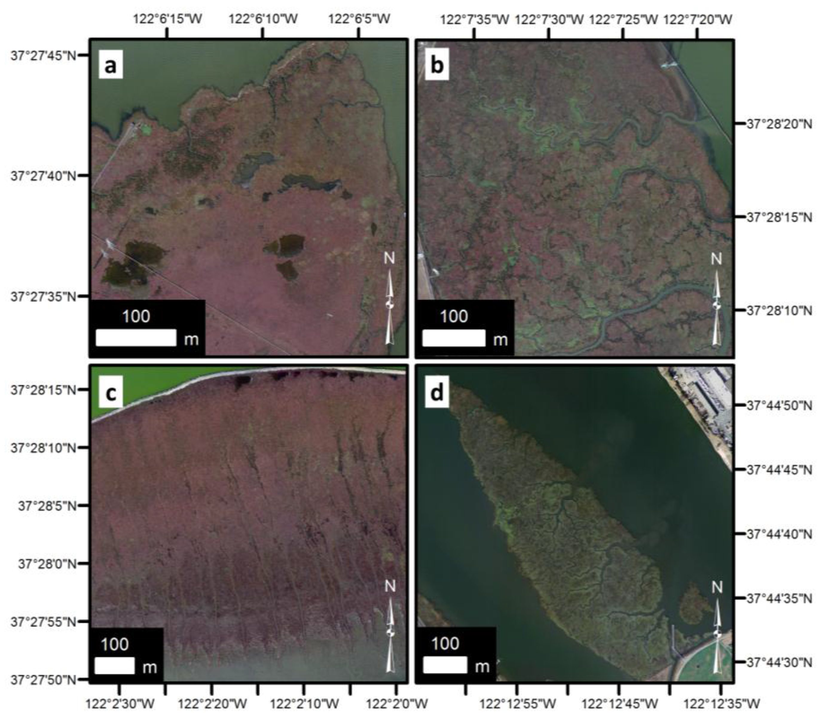
4.3. Orthophotos Capture Two States among Salt Marshes of San Francisco Bay

Since the long historical record of coastal wetland structure and vegetation that is needed to diagnose the presence of alternative stable states is not always available, in some cases a “space-for-time substitution” approach may be useful [268]. In this approach, one deductively studies differences in environmental patterns and processes among sites thought to represent different ages along a successional or other developmental gradient. Then one can, with caution [269], inductively predict the likely trajectory of development in time that would “connect-the-dots” between the observed intermediate states. This approach to studying state trajectories of coastal wetlands makes sense in cases where many wetlands in the same geographical region of the same ecosystem type have been subjected to the same historical environmental influences. The key is that the set of wetlands should be able to reasonably be assumed to be a representative sample from the population of the many wetland states/development trajectories/outcomes possible for that specific region. The need to select representative sites a priori produces some challenges, however, including possible bias in the initial site selection and likely imperfect sampling of the age gradient. Therefore, the space-for-time substitution approach can be made more robust by including many study sites within each age group studied.

These criteria were met in a study of salt marshes in San Francisco Bay. A set of 77 saline (not brackish) marshes in North (San Pablo), Central, and South San Francisco Bays were categorized based on expert inspection of the vegetation and channel patterns visible in true color, high-resolution (0.3 m) aerial photography from 2004 [270] and ancillary data [271,272]. The ancillary data enabled labeling each marsh with a relative age: Mature (>160 years old), young (<160 years old, established since the California Gold Rush sediment pulse), or recently restored (1930–2002).

The marsh vegetation pattern categories were labeled based on visual inspection of marsh color and texture in the true-color imagery as generally complex, simple, or developing vegetation. The complex vegetation pattern categories were: (a) mosaic (many colors interspersed as complex array of patches); and (b) mosaic-solid (mostly one color, but with strong patchiness or patchiness over a large area). The simple vegetation pattern categories were: (c) solid (mostly one color, minor or absent patchiness); (d) banded (prominent bands of color oriented parallel to the shoreline, i.e., classic zonation relative to shoreline); and (e) simple solid-banded (mostly one color, minor or absent banding). The final vegetation class was: (f) developing (mostly water or mudflat, but with small patches of vegetation on mudflat or lining channel banks).

The marsh channel pattern categories were labeled based on visual inspection of channel sinuosity and network connectivity as generally complex, simple, or anthropogenic. The complex channel pattern categories were: (a) dendritic (naturally sinuous channels with clear branching pattern); and (b) dendritic-looped (naturally sinuous channels with clear branching pattern, some of which loop back to connect to the same or adjacent drainage network). The simple channel pattern categories were: (c) perpendicular (naturally wavy/straight channels oriented perpendicular to shoreline); and (d) none (no apparent channels). Alternatively, some marshes had clearly anthropogenic channels, established by historical ditching for drainage or borrow ditches from which sediment was taken to form levees.

Overall, literature and ecological theory imply a prevailing hypothesis that more mature marshes develop more complex vegetation and channel patterns over time. Largely contrary to this hypothesis, in this study most vegetation and channel pattern classes were well-represented in marshes of all age groups (Figure 8). The most simple (solid, solid-banded, or banded) vegetation patterns were found in about 38%, 59% and 33% of mature, young, and restored marshes, respectively. An additional 25% of restored marshes only exhibited the developing vegetation as of the time of the imagery. The balance of marshes exhibited the complex (mosaic or mosaic-solid) vegetation patterns, in about 62%, 41% and 42% of mature, young, and restored marshes, respectively. Marshes of all age groups also exhibited each nearly every type of channel pattern. Anthropogenic channels dominated about 19%, 24% and 29% of mature, young, and restored marshes, respectively. Marshes with simple channels accounted for about 23%, 41% and 8% of mature, young, and restored marshes, respectively. The balance of marshes exhibited complex channel patterns, in about 58%, 34% and 42% of mature, young, and restored marshes, respectively. Furthermore, the vegetation and channel pattern of a marsh typically corresponded, with marshes either displaying complex vegetation and complex channel patterns or simple vegetation and simple channel patterns. For example, among just complex and simple vegetation and channel patterns, 76% of marshes with complex channel patterns had complex vegetation patterns and 75% of marshes with simple channel patterns had simple vegetation patterns.

Figure 8. Salt marshes in San Francisco Bay. (a) Mature marsh with simple vegetation and channel patterns (Sand Point, Palo Alto); (b) Mature marsh with complex vegetation and channel patterns (Laumeister Tract, East Palo Alto); (c) Young marsh with simple vegetation and channel patterns (Arrowhead Marsh, Oakland); and (d) Young marsh with complex vegetation and channel patterns (Laumeister Tract, East Palo Alto). Aerial imagery from [270].

Figure 8. Salt marshes in San Francisco Bay. (a) Mature marsh with simple vegetation and channel patterns (Sand Point, Palo Alto); (b) Mature marsh with complex vegetation and channel patterns (Laumeister Tract, East Palo Alto); (c) Young marsh with simple vegetation and channel patterns (Arrowhead Marsh, Oakland); and (d) Young marsh with complex vegetation and channel patterns (Laumeister Tract, East Palo Alto). Aerial imagery from [270].

These findings suggest a new hypothesis: Instead of increasing channel and vegetation complexity with age, these marshes tend to occupy one of two alternative states. One of these states appears characterized by complex vegetation and channel patterns, which likely form in an interrelated manner, and the other state appears characterized by simple vegetation and channel patterns. That the patterns are stable over time, rather than frequently switching from one to the other, is suggested by this interrelationship, as channels tend to be quite stationary once established in salt marshes, even if vegetation might change year-to-year given disturbance. The stability of marshes in each of the two states is also corroborated by the representation of both simple and complex vegetation and channel types in multiple marshes of each age group. Quantitative analysis and testing of this new hypothesis and examination of its relationship to marsh slope, hydrology, and sediment accretion rate is ongoing.

5. Further Research Needs and Opportunities

Clearly, a wealth of mathematical theory and numerical modeling is available to aid in posing hypotheses regarding multiple stable states in coastal wetlands. However, substantial investment in empirical validation is still required to demonstrate whether multiple stable state theory holds generally in the coastal zone, only for specific sites, or not well at all, upon empirical testing. Special attention should be paid to the regions where large areas of transition between states have appeared, and especially to the regions that have transferred forwards and backwards between two states. Empirical studies should be carried out to test the indicators of alternative stable states, such as abrupt shifts, sharp boundaries, bimodality, and hysteresis. Repeated monitoring over long time frames is similarly crucial to properly validate long-term stability of observed states. The recent success in using remote sensing to test hypotheses at ecosystem scales could be leveraged substantially more to address key research needs and challenges in this field. Meanwhile, experimental studies at the plant, patch, and plot scales in laboratory flumes, greenhouses, and in the field will continue to deepen understanding of detailed processes in coastal wetlands.

Here we enumerate some key research challenges to advance understanding of potential alternative stable states in coastal wetlands. Remote sensing approaches may prove useful in many of these avenues.

5.1. Theory and Models Need to Be Made Spatially Explicit and Species Explicit

A real leap forward in understanding more complex and realistic ecosystem change, intra-ecosystem habitat and patchiness, and system heterogeneity requires two- and three-dimensional, spatially explicit theory and modeling. So far, numerical models that simulate alternative coastal wetland stable states have mostly been zero- or one-dimensional, e.g., assessing the factors driving coupled and topographic change at a given hypothetical point or entire marsh area in the intertidal zone. While moving beyond one-point-wetland models, understanding differences in the ecosystem engineering roles of multiple major coastal wetland plant species is also critical. High-resolution remote sensing can provide spatially distributed input data for distributed models (e.g., digital elevation models, snapshots that can be used for initial conditions or validation time points) and aid in mapping specific vegetation distributions. Studies of “The Spatial Mosaic” [153] are as relevant and challenging as ever.

5.2. The Relative Roles of Biotic vs. Abiotic Factors Need to Be Better Quantified

It is widely understood that the organization of coastal wetlands depends on both biotic and abiotic factors and the interactions among them. These interactions are captured in current theory via simple linear and non-linear models, e.g., of sediment settling or biomass growth, but the nature and strengths of such interactions are generally set by a priori assumptions. Although the precise nature of these interactions are likely to be site-specific, progress is needed toward quantifying the roles and interactions of biotic and abiotic factors in driving tendencies for alternative stable states, to better tie theory to reality. Remote sensing analysis can aid in this effort, e.g., by using different band combinations in multispectral imagery to highlight spatial and temporal dynamics of abiotic (e.g., sediment) vs. biotic (e.g., green vegetation) ecosystem components.

5.3. Multi-Species, Multi-State Dynamics Need to Be Tied to Specific Biological Interactions

Key biological interactions in ecosystems include predation, herbivory, competition, facilitation, host-pest/parasite relations, succession, and disturbance. Herbivory, predation, pests, and parasites were prominently considered in the seminal application of multiple stable state theory to populations (e.g., [111,153]). Competition between species has been examined in a few cases in terrestrial peatlands [125] and on coral reefs [127], although these analyses have generally lacked a spatial component. Spatial competition for scarce water and nutrients among individuals of the same vegetation type has been examined extensively for arid and semi-arid ecosystems (e.g., [109,133,134,135,136,137,138,139,140]), but there is ample opportunity to examine multiple-species systems. More neutral or even facilitative interactions are suggested by the spatial redistribution of water and nutrients to hummocks in peatlands [120]. If hollows were shown to be “active” participants in this redistribution, then the patterned, coexisting stable states might be said to arise from a mutualism. State shifts induced by disturbance, whether by humans or other organisms, might be framed in terms of amensalism, but the strict applicability of the term would need to be tested. Early successional plant species might promote their competitive position by modifying the environment in their favor and therefore slow down the succession process and lock the ecosystem in an early state for a long time [273]. Disturbance-driven ecosystems, such as some salt marshes, mangroves, floodplain, and dune systems, may exhibit “windows of opportunity.” These “windows” are disturbance-free periods of a minimal duration that directly follow diaspore dispersal and allow seedling establishment, and therefore may help induce a sudden shift from bare to a vegetated state as predicted and validated with remote sensing [274]. The combination of predation, competition for space, and facilitation of recruitment has been examined among multiple species on reefs [126]. As such multiple-biological interactions are already well understood in the ecological literature, it remains to further extend and apply that knowledge base to provide mechanistic underpinnings for cases in which multiple stable coastal wetland ecosystem states can be empirically documented.

5.4. Analysis Needs to Extend to Open Systems, with Differences and Similarities between Closed and Open Systems Appreciated

The initial application of multiple stable state theory as a framework for catastrophic shifts in lacustrine systems was immensely successful in large part because the lakes could be treated as largely closed systems [153]. By extension, can partly-open coastal embayments or fully-open shoreline systems exhibit similar dynamics under certain conditions? By way of convenience, coastal wetlands are often treated as closed systems in modeling their states, but an important area of inquiry would test relaxing this assumption. To extend observations offshore and so support “opening” the boundary of these models, remote sensing is likely to be particularly useful, e.g., to track movement of related sediment plumes or phytoplankton blooms toward or away from shore.

5.5. The Distinction between True Ecosystem Self-Organization, Reliant on Internal Feedbacks, and Other Causes of Complex Ecosystem Patterning Needs to Be Clarified and More Strictly and Critically Examined in Applications

Given the elegance of multiple stable state theory and the related concept of self-organized ecosystem patterning, it is tempting to invoke these theories to explain a wide variety of environmental observations. However, the degree to which this is justified could be examined in greater detail. For example, the ability to fit a power-law curve to empirical data on vegetation patch size is compelling, but not in itself final evidence that scale-dependent processes are responsible for those patch sizes, nor that they truly produce scale-free ecosystem self-organization. A process-based understanding based in spatially extensive observations over time, rather than statistical analysis of snapshots in space or time, is preferable and needed and would be valuably supported by remote sensing data inputs. Similarly, a greater emphasis on high temporal and spatial resolution analysis should aid in discriminating between ecosystem phase shifts vs. state oscillations vs. true switches between alternative stable states.

5.6. The Scaling Relationships between Ecosystem Scale Processes and the Patch-Scale Processes Observable in Laboratories, Greenhouses, and Field Plots Need to Be Determined

Plant and patch scale observations in laboratory flumes and intensively monitored field plots will continue to advance mechanistic understandings of coastal wetland community and morphodynamic change. Remote sensing holds the promise of documenting ecosystem- and coastline-scale state dynamics over time. Although the existence of multiple states at one scale does not require multiple states to exist at other scales [156], there must be connections that describe how fine processes aggregate to coarse patterns, which still require elucidation.

6. Conclusions

To inform large scale and long term adaptive coastal management and restoration, high-resolution, ecosystem-scale observation over extended spatial and temporal scales is a critical need. Such data can be highly useful in empirically testing hypothesized alternative stable states in coastal wetlands. To date, only a few studies have used remotely sensed data to try to quantitatively validate the presence of alternative stable states in coastal wetlands: Three studies in salt marshes [86,216], three in deltas [188,189,225], one in mangroves [264], and perhaps three in seagrasses [252,257,260], including the examples presented in Section 4. These studies are suggestive of the promise of using remotely sensed data to test alternative stable state hypotheses, but extensive and thorough testing for coastal environments and regular, accepted testing approaches and quantitative state metrics are so far lacking.

Whether coastal wetland stability, resilience, and change are accurately described by the theory of alternative stable states has very real consequences for practical science and management in the coastal zone. If alternative stable states are a reality, developing knowledge and methods to predict and avoid catastrophic state shifts are key, as is planning restoration efforts to allow the coastal wetland system to evolve into the desired stable end point. Also, adaptive management strategies may be ineffective against external triggers of catastrophic state shifts. If alternative stable state theory does not strictly hold for a coastal wetland, then managers can plan conservation, management, and restoration according to more incremental and gradual adaptive management approaches. In either case, remote sensing is an ideally suited approach to provide data in making the assessment of whether alternative stable state theory applies, and to monitor wetland change over time. Still, considering the typically long time scales that may be required to fully identify multiple stable states in coastal systems, especially at the ecosystem scale, it is difficult to find long enough remote sensing datasets. Therefore, inventive approaches for using existing long-term data and space-for-time substitution techniques, as well as continuous investment in acquisition of new imagery, are all critical research and civil activities.

References

1. USGS. Delta Research and Global Observation Network (DRAGON). Available online: http://deltas.usgs.gov/ (accessed on 24 April 2015).
2. Pendleton, L.; Donato, D.C.; Murray, B.C.; Crooks, S.; Jenkins, W.A.; Sifleet, S.; Craft, C.; Fourqurean, J.W.; Kauffman, J.B.; Marbà, N.; et al. A. Estimating global “blue carbon” emissions from conversion and degradation of vegetated coastal ecosystems. PLoS ONE 2012, 7, e43542. [Google Scholar]
3. IGPB. Deltas at Risk—IGBP. Available online: http://www.igbp.net/multimedia/multimedia/deltasatrisk.5.62dc35801456272b46d351.html (accessed on 24 April 2015).
4. Kirwan, M.L.; Murray, A.B.; Donnelly, J.P.; Corbett, D.R. Rapid wetland expansion during European settlement and its implication for marsh survival under modern sediment delivery rates. Geology 2011, 39, 507–510. [Google Scholar]
5. Coverdale, T.C.; Herrmann, N.C.; Altieri, A.H.; Bertness, M.D. Latent impacts: The role of historical human activity in coastal habitat loss. Front. Ecol. Environ. 2013, 11, 69–74. [Google Scholar]
6. Creel, L. Ripple Effects: Population and Coastal Regions; Population Reference Bureau: Washington, DC, USA, 2003. [Google Scholar]
7. Temmerman, S.; Meire, P.; Bouma, T.J.; Herman, P.M.J.; Ysebaert, T.; de Vriend, H.J. Ecosystem-based coastal defence in the face of global change. Nature 2013, 504, 79–83. [Google Scholar]
8. Byrne, R.; Ingram, B.L.; Starratt, S.; Malamud-Roam, F.; Collins, J.N.; Conrad, M.E. Carbon-isotope, diatom, and pollen evidence for late holocene salinity change in a brackish marsh in the San Francisco estuary. Quat. Res. 2001, 55, 66–76. [Google Scholar]
9. Malamud-Roam, F.; Lynn Ingram, B. Late Holocene δ13C and pollen records of paleosalinity from tidal marshes in the San Francisco Bay estuary, California. Quat. Res. 2004, 62, 134–145. [Google Scholar]
10. Kemp, A.C.; Bernhardt, C.E.; Horton, B.P.; Kopp, R.E.; Vane, C.H.; Peltier, W.R.; Hawkes, A.D.; Donnelly, J.P.; Parnell, A.C.; Cahill, N. Late Holocene sea- and land-level change on the U.S. southeastern Atlantic coast. Mar. Geol. 2014, 357, 90–100. [Google Scholar]
11. Bolshiyanov, D.; Makarov, A.; Savelieva, L. Lena River delta formation during the Holocene. Biogeosciences 2015, 12, 579–593. [Google Scholar] [CrossRef]
12. Brain, M.J.; Kemp, A.C.; Horton, B.P.; Culver, S.J.; Parnell, A.C.; Cahill, N. Quantifying the contribution of sediment compaction to late Holocene salt-marsh sea-level reconstructions, North Carolina, USA. Quat. Res. 2015, 83, 41–51. [Google Scholar] [CrossRef] [Green Version]
13. Stéphan, P.; Goslin, J.; Pailler, Y.; Manceau, R.; Suanez, S.; Van Vliet-Lanoë, B.; Hénaff, A.; Delacourt, C. Holocene salt-marsh sedimentary infilling and relative sea-level changes in West Brittany (France) using foraminifera-based transfer functions. Boreas 2015, 44, 153–177. [Google Scholar] [CrossRef] [Green Version]
14. Simas, T.; Nunes, J.P.; Ferreira, J.G. Effects of global climate change on coastal salt marshes. Ecol. Model. 2001, 139, 1–15. [Google Scholar] [CrossRef]
15. Cahoon, D.R.; Hensel, P.F.; Spencer, T.; Reed, D.J.; McKee, K.L.; Saintilan, N. Coastal wetland vulnerability to relative sea-level rise: Wetland elevation trends and process controls. In Wetlands and Natural Resource Management; Springer: Berlin, Germany, 2006; pp. 271–292. [Google Scholar]
16. Blume, H.P.; Müller-Thomsen, U. A field experiment on the influence of the postulated global climatic change on coastal marshland soils. J. Plant Nutr. Soil Sci. 2007, 170, 145–156. [Google Scholar] [CrossRef]
17. Day, J.W.; Christian, R.R.; Boesch, D.M.; Yáñez-Arancibia, A.; Morris, J.; Twilley, R.R.; Naylor, L.; Schaffner, L.; Stevenson, C. Consequences of Climate Change on the Ecogeomorphology of Coastal Wetlands. Estuaries Coasts 2008, 31, 477–491. [Google Scholar] [CrossRef]
18. Kirwan, M.L.; Murray, A.B. Tidal marshes as disequilibrium landscapes? Lags between morphology and Holocene sea level change. Geophys. Res. Lett. 2008, 35. [Google Scholar] [CrossRef]
19. Craft, C.; Clough, J.; Ehman, J.; Joye, S.; Park, R.; Pennings, S.; Guo, H.; Machmuller, M. Forecasting the effects of accelerated sea-level rise on tidal marsh ecosystem services. Front. Ecol. Environ. 2009, 7, 73–78. [Google Scholar] [CrossRef]
20. Kirwan, M.L.; Guntenspergen, G.R.; D’Alpaos, A.; Morris, J.T.; Mudd, S.M.; Temmerman, S. Limits on the adaptability of coastal marshes to rising sea level. Geophys. Res. Lett. 2010, 37, L23401. [Google Scholar] [CrossRef]
21. Kirwan, M.L.; Megonigal, J.P. Tidal wetland stability in the face of human impacts and sea-level rise. Nature 2013, 504, 53–60. [Google Scholar] [CrossRef] [PubMed]
22. Costanza, R.; D’Arge, R.; de Groot, R.; Farber, S.; Grasso, M.; Hannon, B.; Limburg, K.; Naeem, S.; O’Neill, R.V.; Paruelo, J.; et al. The value of the world’s ecosystem services and natural capital. Nature 1997, 387, 253–260. [Google Scholar] [CrossRef]
23. Woodward, R.T.; Wui, Y.S. The economic value of wetland services: A meta-analysis. Ecol. Econ. 2001, 37, 257–270. [Google Scholar] [CrossRef]
24. Tol, R.S.J. The double trade-off between adaptation and mitigation for sea level rise: An application of FUND. Mitig. Adapt. Strateg. Glob. Change 2007, 12, 741–753. [Google Scholar] [CrossRef]
25. Costanza, R.; Pérez-Maqueo, O.; Martinez, M.L.; Sutton, P.; Anderson, S.J.; Mulder, K. The value of coastal wetlands for hurricane protection. AMBIO J. Hum. Environ. 2008, 37, 241–248. [Google Scholar] [CrossRef]
26. Gedan, K.B.; Kirwan, M.L.; Wolanski, E.; Barbier, E.B.; Silliman, B.R. The present and future role of coastal wetland vegetation in protecting shorelines: Answering recent challenges to the paradigm. Clim. Change 2011, 106, 7–29. [Google Scholar] [CrossRef]
27. Möller, I.; Kudella, M.; Rupprecht, F.; Spencer, T.; Paul, M.; van Wesenbeeck, B.K.; Wolters, G.; Jensen, K.; Bouma, T.J.; Miranda-Lange, M.; et al. Wave attenuation over coastal salt marshes under storm surge conditions. Nat. Geosci. 2014, 7, 727–731. [Google Scholar] [CrossRef]
28. Mcleod, E.; Chmura, G.L.; Bouillon, S.; Salm, R.; Björk, M.; Duarte, C.M.; Lovelock, C.E.; Schlesinger, W.H.; Silliman, B.R. A blueprint for blue carbon: Toward an improved understanding of the role of vegetated coastal habitats in sequestering CO2. Front. Ecol. Environ. 2011, 9, 552–560. [Google Scholar] [CrossRef] [Green Version]
29. Bauer, J.E.; Cai, W.J.; Raymond, P.A.; Bianchi, T.S.; Hopkinson, C.S.; Regnier, P.A.G. The changing carbon cycle of the coastal ocean. Nature 2013, 504, 61–70. [Google Scholar] [CrossRef] [PubMed]
30. Duarte, C.M.; Losada, I.J.; Hendriks, I.E.; Mazarrasa, I.; Marbà, N. The role of coastal plant communities for climate change mitigation and adaptation. Nat. Clim. Change 2013, 3, 961–968. [Google Scholar] [CrossRef]
31. Mitsch, W.J.; Gosselink, J.G. Wetlands, 4th ed.; Wiley: Hoboken, NJ, USA, 2007. [Google Scholar]
32. Yang, M.; Geng, X.; Grace, J.; Lu, C.; Zhu, Y.; Zhou, Y.; Lei, G. Spatial and Seasonal CH4 Flux in the Littoral Zone of Miyun Reservoir near Beijing: The Effects of Water Level and Its Fluctuation. PLoS ONE 2014, 9, e94275. [Google Scholar] [CrossRef] [PubMed]
33. Poffenbarger, H.J.; Needelman, B.A.; Megonigal, J.P. Salinity Influence on Methane Emissions from Tidal Marshes. Wetlands 2011, 31, 831–842. [Google Scholar] [CrossRef]
34. Kneib, R.T.; Wagner, S.L. Nekton use of vegetated marsh habitats at different stages of tidal inundation. Mar. Ecol. Prog. Ser. 1994, 106, 227–238. [Google Scholar] [CrossRef]
35. Minello, T.J.; Rozas, L.P. Nekton in Gulf Coast wetlands: Fine-scale distributions, landscape patterns, and restoration implications. Ecol. Appl. 2002, 12, 441–455. [Google Scholar] [CrossRef]
36. Bretsch, K.; Allen, D.M. Tidal migrations of nekton in salt marsh intertidal creeks. Estuaries Coasts 2006, 29, 474–486. [Google Scholar] [CrossRef]
37. UNEP-WCMC. Ocean Data Viewer. Available online: http://data.unep-wcmc.org/ (accessed on 24 April 2015).
38. US FWS. National Wetlands Inventory. Available online: http://www.fws.gov/wetlands/index.html (accessed on 24 April 2015).
39. Kirwan, M.L.; Murray, A.B. A coupled geomorphic and ecological model of tidal marsh evolution. Proc. Natl. Acad. Sci. USA 2007, 104, 6118–6122. [Google Scholar] [CrossRef] [PubMed]
40. Marani, M.; D’Alpaos, A.; Lanzoni, S.; Carniello, L.; Rinaldo, A. Biologically-controlled multiple equilibria of tidal landforms and the fate of the Venice lagoon. Geophys. Res. Lett. 2007, 34. [Google Scholar] [CrossRef]
41. Marani, M.; D’Alpaos, A.; Lanzoni, S.; Carniello, L.; Rinaldo, A. The importance of being coupled: Stable states and catastrophic shifts in tidal biomorphodynamics. J. Geophys. Res. Earth Surf. 2010, 115, F04004. [Google Scholar] [CrossRef]
42. Marani, M.; da Lio, C.; D’Alpaos, A. Vegetation engineers marsh morphology through multiple competing stable states. Proc. Natl. Acad. Sci. USA 2013, 110, 3259–3263. [Google Scholar] [CrossRef] [PubMed]
43. Fagherazzi, S.; Kirwan, M.L.; Mudd, S.M.; Guntenspergen, G.R.; Temmerman, S.; D’Alpaos, A.; van de Koppel, J.; Rybczyk, J.M.; Reyes, E.; Craft, C.; et al. Numerical models of salt marsh evolution: Ecological, geomorphic, and climatic factors. Rev. Geophys. 2012, 50, RG1002. [Google Scholar] [CrossRef]
44. Osman, R.W.; Munguia, P.; Zajac, R.N. Ecological thresholds in marine communities: Theory, experiments and mangement. Mar. Ecol. Prog. Ser. 2010, 413, 185–187. [Google Scholar] [CrossRef]
45. Thrush, S.F.; Hewitt, J.E.; Lohrer, A.M. Interaction networks in coastal soft-sediments highlight the potential for change in ecological resilience. Ecol. Appl. 2012, 22, 1213–1223. [Google Scholar] [CrossRef] [PubMed]
46. Williams, P.; Faber, P. Salt marsh restoration experience in San Francisco Bay. J. Coast. Res. 2001, 27, 203–211. [Google Scholar]
47. Williams, P.B.; Orr, M.K. Physical evolution of restored breached levee salt marshes in the San Francisco Bay estuary. Restor. Ecol. 2002, 10, 527–542. [Google Scholar] [CrossRef]
48. Hughes, R.G.; Paramor, O.A.L. On the loss of saltmarshes in south-east England and methods for their restoration. J. Appl. Ecol. 2004, 41, 440–448. [Google Scholar] [CrossRef]
49. Palmer, M.A. Reforming watershed restoration: Science in need of application and applications in need of science. Estuaries Coasts 2008, 32, 1–17. [Google Scholar] [CrossRef]
50. Ozesmi, S.L.; Bauer, M.E. Satellite remote sensing of wetlands. Wetl. Ecol. Manag. 2002, 10, 381–402. [Google Scholar] [CrossRef]
51. Silva, T.S.F.; Costa, M.P.F.; Melack, J.M.; Novo, E.M.L.M. Remote sensing of aquatic vegetation: Theory and applications. Environ. Monit. Assess. 2007, 140, 131–145. [Google Scholar] [CrossRef] [PubMed]
52. Xie, Y.; Sha, Z.; Yu, M. Remote sensing imagery in vegetation mapping: A review. J. Plant Ecol. 2008, 1, 9–23. [Google Scholar] [CrossRef]
53. Klemas, V. Remote sensing techniques for studying coastal ecosystems: An overview. J. Coast. Res. 2010, 27, 2–17. [Google Scholar] [CrossRef]
54. Bartlett, D.S.; Klemas, V. Quantitative assessment of tidal wetlands using remote sensing. Environ. Manag. 1980, 4, 337–345. [Google Scholar] [CrossRef]
55. Bartlett, D.; Klemas, V. In situ spectral reflectance studies of tidal wetland grasses. Photogramm. Eng. Remote Sens. 1981, 47, 1695–1703. [Google Scholar]
56. Silvestri, S.; Marani, M.; Marani, A. Hyperspectral remote sensing of salt marsh vegetation, morphology and soil topography. Phys. Chem. Earth Parts ABC 2003, 28, 15–25. [Google Scholar] [CrossRef]
57. Ustin, S.L.; Roberts, D.A.; Gamon, J.A.; Asner, G.P.; Green, R.O. Using imaging spectroscopy to study ecosystem processes and properties. BioScience 2004, 54, 523–534. [Google Scholar] [CrossRef]
58. Li, L.; Ustin, S.L.; Lay, M. Application of multiple endmember spectral mixture analysis (MESMA) to AVIRIS imagery for coastal salt marsh mapping: A case study in China Camp, CA, USA. Int. J. Remote Sens. 2005, 26, 5193–5207. [Google Scholar] [CrossRef]
59. Rosso, P.H.; Ustin, S.L.; Hastings, A. Mapping marshland vegetation of San Francisco Bay, California, using hyperspectral data. Int. J. Remote Sens. 2005, 26, 5169–5191. [Google Scholar] [CrossRef]
60. Artigas, F.J.; Yang, J. Spectral discrimination of marsh vegetation types in the New Jersey Meadowlands, USA. Wetlands 2006, 26, 271–277. [Google Scholar] [CrossRef]
61. Gao, Z.G.; Zhang, L.Q. Multi-seasonal spectral characteristics analysis of coastal salt marsh vegetation in Shanghai, China. Estuar. Coast. Shelf Sci. 2006, 69, 217–224. [Google Scholar] [CrossRef]
62. Judd, C.; Steinberg, S.; Shaughnessy, F.; Crawford, G. Mapping salt marsh vegetation using aerial hyperspectral imagery and linear unmixing in Humboldt Bay, California. Wetlands 2007, 27, 1144–1152. [Google Scholar] [CrossRef]
63. Sadro, S.; Gastil-Buhl, M.; Melack, J. Characterizing patterns of plant distribution in a southern California salt marsh using remotely sensed topographic and hyperspectral data and local tidal fluctuations. Remote Sens. Environ. 2007, 110, 226–239. [Google Scholar] [CrossRef]
64. Gilmore, M.S.; Wilson, E.H.; Barrett, N.; Civco, D.L.; Prisloe, S.; Hurd, J.D.; Chadwick, C. Integrating multi-temporal spectral and structural information to map wetland vegetation in a lower Connecticut River tidal marsh. Remote Sens. Environ. 2008, 112, 4048–4060. [Google Scholar] [CrossRef]
65. Miyamoto, M.; Kushida, K.; Yoshino, K.; Nagano, T.; Sato, Y. Evaluation of multispatial scale measurements for monitoring wetland vegetation, Kushiro wetland, Japan: Application of SPOT images, CASI data, airborne CNIR video images and balloon aerial photography. IEEE Geosci. Remote Sens. Symp. 2003, 5, 3275–3277. [Google Scholar]
66. Wang, L.; Sousa, W.P.; Gong, P.; Biging, G.S. Comparison of IKONOS and QuickBird images for mapping mangrove species on the Caribbean coast of Panama. Remote Sens. Environ. 2004, 91, 432–440. [Google Scholar] [CrossRef]
67. Belluco, E.; Camuffo, M.; Ferrari, S.; Modenese, L.; Silvestri, S.; Marani, A.; Marani, M. Mapping salt-marsh vegetation by multispectral and hyperspectral remote sensing. Remote Sens. Environ. 2006, 105, 54–67. [Google Scholar] [CrossRef]
68. Klemas, V. Airborne remote sensing of coastal features and processes: An overview. J. Coast. Res. 2012, 29, 239–255. [Google Scholar] [CrossRef]
69. Moffett, K.B.; Gorelick, S.M. Distinguishing wetland vegetation and channel features with object-based image segmentation. Int. J. Remote Sens. 2013, 34, 1332–1354. [Google Scholar] [CrossRef]
70. Wang, L.; Sousa, W.P.; Gong, P. Integration of object-based and pixel-based classification for mapping mangroves with IKONOS imagery. Int. J. Remote Sens. 2004, 25, 5655–5668. [Google Scholar] [CrossRef]
71. Lathrop, R.G.; Montesano, P.; Haag, S. A multi-scale segmentation approach to mapping seagrass habitats using airborne digital camera imagery. Photogramm. Eng. Remote Sens. 2006, 72, 665–675. [Google Scholar] [CrossRef]
72. Yu, Q.; Gong, P.; Clinton, N.; Biging, G.; Kelly, M.; Schirokauer, D. Object-based detailed vegetation classification with airborne high spatial resolution remote sensing imagery. Photogramm. Eng. Remote Sens. 2006, 72, 799–811. [Google Scholar] [CrossRef]
73. Tian, B.; Zhou, Y.; Zhang, L.; Yuan, L. Analyzing the habitat suitability for migratory birds at the Chongming Dongtan Nature Reserve in Shanghai, China. Estuar. Coast. Shelf Sci. 2008, 80, 296–302. [Google Scholar] [CrossRef]
74. Tuxen, K.; Kelly, M. Multi-scale functional mapping of tidal marsh vegetation using object-based image analysis. In Object-Based Image Analysis; Lecture Notes in Geoinformation and Cartography; Blaschke, T., Lang, S., Hay, G.J., Eds.; Springer: Berlin, Heidelberg, Germany, 2008; pp. 415–442. [Google Scholar]
75. Rokitnicki-Wojcik, D.; Wei, A.; Chow-Fraser, P. Transferability of object-based rule sets for mapping coastal high marsh habitat among different regions in Georgian Bay, Canada. Wetl. Ecol. Manag. 2011, 19, 223–236. [Google Scholar] [CrossRef]
76. Silvestri, S.; Marani, M.; Settle, J.; Benvenuto, F.; Marani, A. Salt marsh vegetation radiometry: Data analysis and scaling. Remote Sens. Environ. 2002, 80, 473–482. [Google Scholar] [CrossRef]
77. Simard, M.; Rivera-Monroy, V.H.; Mancera-Pineda, J.E.; Castañeda-Moya, E.; Twilley, R.R. A systematic method for 3D mapping of mangrove forests based on Shuttle Radar Topography Mission elevation data, ICEsat/GLAS waveforms and field data: Application to Ciénaga Grande de Santa Marta, Colombia. Remote Sens. Environ. 2008, 112, 2131–2144. [Google Scholar] [CrossRef]
78. Kim, M.; Warner, T.A.; Madden, M.; Atkinson, D.S. Multi-scale GEOBIA with very high spatial resolution digital aerial imagery: Scale, texture and image objects. Int. J. Remote Sens. 2011, 32, 2825–2850. [Google Scholar] [CrossRef]
79. Klemas, V.; Daiber, F.; Bartlett, D.; Crichton, O.; Fornes, A. Inventory of Delawares Wetlands. Photogramm. Eng. Remote Sens. 1974, 40, 433–439. [Google Scholar]
80. Hardisky, M.A.; Klemas, V. Tidal wetlands natural and human-made changes from 1973 to 1979 in Delaware: Mapping techniques and results. Environ. Manag. 1983, 7, 339–344. [Google Scholar] [CrossRef]
81. Zharikov, Y.; Skilleter, G.A.; Loneragan, N.R.; Taranto, T.; Cameron, B.E. Mapping and characterising subtropical estuarine landscapes using aerial photography and GIS for potential application in wildlife conservation and management. Biol. Conserv. 2005, 125, 87–100. [Google Scholar] [CrossRef]
82. Prigent, C.; Matthews, E.; Aires, F.; Rossow, W.B. Remote sensing of global wetland dynamics with multiple satellite data sets. Geophys. Res. Lett. 2001, 28, 4631–4634. [Google Scholar] [CrossRef]
83. Prigent, C.; Papa, F.; Aires, F.; Rossow, W.B.; Matthews, E. Global inundation dynamics inferred from multiple satellite observations, 1993–2000. J. Geophys. Res. 2007, 112. [Google Scholar] [CrossRef]
84. Feola, A. A geomorphic study of lagoonal landforms. Water Resour. Res. 2005, 41. [Google Scholar] [CrossRef]
85. Klemas, V. Remote sensing of emergent and submerged wetlands: An overview. Int. J. Remote Sens. 2013, 34, 6286–6320. [Google Scholar] [CrossRef]
86. Wang, C.; Temmerman, S. Does biogeomorphic feedback lead to abrupt shifts between alternative landscape states? An empirical study on intertidal flats and marshes. J. Geophys. Res. Earth Surf. 2013, 118, 229–240. [Google Scholar] [CrossRef]
87. Zhang, M.; Ustin, S.L.; Rejmankova, E.; Sanderson, E.W. Monitoring Pacific coast salt marshes using remote sensing. Ecol. Appl. 1997, 7, 1039–1053. [Google Scholar] [CrossRef]
88. Ustin, S.L.; Lay, M.C.; Li, L. Remote sensing of wetland conditions in West Coast salt marshes. SPIE Remote Sens. Model. Ecosyst. Sustain. 2004, 5544. [Google Scholar] [CrossRef]
89. Wilson, M.D.; Ustin, S.L.; Rocke, D.M. Classification of contamination in salt marsh plants using hyperspectral reflectance. IEEE Trans. Geosci. Remote Sens. 2004, 42, 1088–1095. [Google Scholar] [CrossRef]
90. Tilley, D.R.; Ahmed, M.; Son, J.H.; Badrinarayanan, H. Hyperspectral reflectance response of freshwater macrophytes to salinity in a brackish subtropical marsh. J. Environ. Qual. 2007, 36, 780–789. [Google Scholar] [CrossRef] [PubMed]
91. Smith, G.M.; Spencer, T.; Murray, A.L.; French, J.R. Assessing seasonal vegetation change in coastal wetlands with airborne remote sensing: An outline methodology. Mangroves Salt Marshes 1998, 2, 15–28. [Google Scholar] [CrossRef]
92. Krause, G.; Bock, M.; Weiers, S.; Braun, G. Mapping land-cover and mangrove structures with remote sensing techniques: A contribution to a synoptic GIS in support of coastal management in North Brazil. Environ. Manag. 2004, 34, 429–440. [Google Scholar] [CrossRef] [PubMed]
93. Hilbert, K.W. Land cover change within the Grand Bay National Estuarine Research Reserve: 1974–2001. J. Coast. Res. 2006, 226, 1552–1557. [Google Scholar] [CrossRef]
94. Jefferies, R.L.; Jano, A.P.; Abraham, K.F. A biotic agent promotes large-scale catastrophic change in the coastal marshes of Hudson Bay. J. Ecol. 2006, 94, 234–242. [Google Scholar] [CrossRef]
95. Nielsen, E.M.; Prince, S.D.; Koeln, G.T. Wetland change mapping for the U.S. mid-Atlantic region using an outlier detection technique. Remote Sens. Environ. 2008, 112, 4061–4074. [Google Scholar] [CrossRef]
96. Van der Wal, D.; Wielemaker-van den Dool, A.; Herman, P.M.J. Spatial patterns, rates and mechanisms of saltmarsh cycles (Westerschelde, The Netherlands). Estuar. Coast. Shelf Sci. 2008, 76, 357–368. [Google Scholar] [CrossRef]
97. Kelly, M.; Tuxen, K.A.; Stralberg, D. Mapping changes to vegetation pattern in a restoring wetland: Finding pattern metrics that are consistent across spatial scale and time. Ecol. Indic. 2011, 11, 263–273. [Google Scholar] [CrossRef]
98. Andrew, M.; Ustin, S. The role of environmental context in mapping invasive plants with hyperspectral image data. Remote Sens. Environ. 2008, 112, 4301–4317. [Google Scholar] [CrossRef]
99. Peterson, C.H. Does a rigorous criterion for environmental identity preclude the existence of multiple stable points? Am. Nat. 1984, 127–133. [Google Scholar] [CrossRef]
100. Schröder, A.; Persson, L.; de Roos, A.M. Direct experimental evidence for alternative stable states: A review. Oikos 2005, 110, 3–19. [Google Scholar]
101. Dudgeon, S.R.; Aronson, R.B.; Bruno, J.F.; Precht, W.F. Phase shifts and stable states on coral reefs. Mar. Ecol. Prog. Ser. 2010, 413, 201–216. [Google Scholar]
102. Aronson, R.B.; Macintyre, I.G.; Wapnick, C.M.; O’Neill, M.W. Phase shifts, alternative states, and the unprecedented convergence of two reef systems. Ecology 2004, 85, 1876–1891. [Google Scholar]
103. Norstrm, A.V.; Nystrm, M.; Lokrantz, J.; Folke, C. Alternative states on coral reefs: Beyond coral—Macroalgal phase shifts. Mar. Ecol. Prog. Ser. 2009, 376, 295–306. [Google Scholar]
104. Petraitis, P.S.; Hoffman, C. Multiple stable states and relationship between thresholds in processes and states. Mar. Ecol. Prog. Ser. 2010, 413, 189–200. [Google Scholar]
105. Scheffer, M.; Carpenter, S.; Foley, J.A.; Folke, C.; Walker, B. Catastrophic shifts in ecosystems. Nature 2001, 413, 591–596. [Google Scholar] [PubMed]
106. Scheffer, M.; Carpenter, S.R. Catastrophic regime shifts in ecosystems: Linking theory to observation. Trends Ecol. Evol. 2003, 18, 648–656. [Google Scholar]
107. Rietkerk, M.; Dekker, S.C.; de Ruiter, P.C.; van de Koppel, J. Self-organized patchiness and catastrophic shifts in ecosystems. Science 2004, 305, 1926–1929. [Google Scholar] [CrossRef] [PubMed]
108. Scheffer, M.; Bascompte, J.; Brock, W.A.; Brovkin, V.; Carpenter, S.R.; Dakos, V.; Held, H.; van Nes, E.H.; Rietkerk, M.; Sugihara, G. Early-warning signals for critical transitions. Nature 2009, 461, 53–59. [Google Scholar] [CrossRef] [PubMed]
109. Dakos, V.; Kéfi, S.; Rietkerk, M.; Nes Scheffer, M. Slowing down in spatially patterned ecosystems at the brink of collapse. Am. Nat. 2011, 177, E153–E166. [Google Scholar] [CrossRef] [PubMed]
110. May, R.M. Biological populations with nonoverlapping generations: Stable points, stable cycles, and chaos. Science 1974, 186, 645–647. [Google Scholar] [CrossRef] [PubMed]
111. May, R.M. Thresholds and breakpoints in ecosystems with a multiplicity of stable states. Nature 1977, 269, 471–477. [Google Scholar] [CrossRef]
112. May, R.M.; Oster, G.F. Bifurcations and dynamic complexity in simple ecological models. Am. Nat. 1976, 573–599. [Google Scholar] [CrossRef]
113. Knowlton, N. Thresholds and multiple stable states in coral reef community dynamics. Am. Zool. 1992, 32, 674–682. [Google Scholar] [CrossRef]
114. Turing, A.M. The chemical basis of morphogenesis. Philos. Trans. R. Soc. Lond. B Biol. Sci. 1952, 237, 37–72. [Google Scholar] [CrossRef]
115. Cross, M.C.; Hohenberg, P.C. Pattern formation outside of equilibrium. Rev. Mod. Phys. 1993, 65, 851–1112. [Google Scholar] [CrossRef]
116. Maini, P.K.; Painter, K.J.; Chau, H.N.P. Spatial pattern formation in chemical and biological systems. J. Chem. Soc. Faraday Trans. 1997, 93, 3601–3610. [Google Scholar] [CrossRef] [Green Version]
117. Shnerb, N.M.; Sarah, P.; Lavee, H.; Solomon, S. Reactive glass and vegetation patterns. Phys. Rev. Lett. 2003, 90, 038101. [Google Scholar] [CrossRef] [PubMed]
118. Meron, E.; Gilad, E.; von Hardenberg, J.; Shachak, M.; Zarmi, Y. Vegetation patterns along a rainfall gradient. Chaos Solitons Fractals 2004, 19, 367–376. [Google Scholar] [CrossRef]
119. Manor, A.; Shnerb, N.M. Dynamical failure of Turing patterns. Europhys. Lett. EPL 2006, 74, 837–843. [Google Scholar] [CrossRef]
120. Eppinga, M.B.; Rietkerk, M.; Borren, W.; Lapshina, E.D.; Bleuten, W.; Wassen, M.J. Regular surface patterning of peatlands: Confronting theory with field data. Ecosystems 2008, 11, 520–536. [Google Scholar] [CrossRef]
121. Rietkerk, M.; van de Koppel, J. Regular pattern formation in real ecosystems. Trends Ecol. Evol. 2008, 23, 169–175. [Google Scholar] [CrossRef] [PubMed]
122. Van de Koppel, J.; Gascoigne, J.C.; Theraulaz, G.; Rietkerk, M.; Mooij, W.M.; Herman, P.M.J. Experimental evidence for spatial self-organization and its emergent effects in mussel bed ecosystems. Science 2008, 322, 739–742. [Google Scholar] [CrossRef] [PubMed]
123. Borgogno, F.; D’Odorico, P.; Laio, F.; Ridolfi, L. Mathematical models of vegetation pattern formation in ecohydrology. Rev. Geophys. 2009, 47, RG1005. [Google Scholar] [CrossRef]
124. Lefever, R.; Barbier, N.; Couteron, P.; Lejeune, O. Deeply gapped vegetation patterns: On crown/root allometry, criticality and desertification. J. Theor. Biol. 2009, 261, 194–209. [Google Scholar] [CrossRef] [PubMed]
125. Pastor, J.; Peckham, B.; Bridgham, S.; Weltzin, J.; Chen, J. Plant community dynamics, nutrient cycling, and alternative stable equilibria in peatlands. Am. Nat. 2002, 160, 553–568. [Google Scholar] [CrossRef] [PubMed]
126. Baskett, M.L.; Salomon, A.K. Recruitment facilitation can drive alternative states on temperate reefs. Ecology 2010, 91, 1763–1773. [Google Scholar] [CrossRef] [PubMed]
127. González-Rivero, M.; Yakob, L.; Mumby, P.J. The role of sponge competition on coral reef alternative steady states. Ecol. Model. 2011, 222, 1847–1853. [Google Scholar] [CrossRef]
128. Fagherazzi, S.; Carniello, L.; D’Alpaos, L.; Defina, A. Critical bifurcation of shallow microtidal landforms in tidal flats and salt marshes. Proc. Natl. Acad. Sci. USA 2006, 103, 8337–8341. [Google Scholar] [CrossRef] [PubMed]
129. Fagherazzi, S.; Palermo, C.; Rulli, M.C.; Carniello, L.; Defina, A. Wind waves in shallow microtidal basins and the dynamic equilibrium of tidal flats. J. Geophys. Res. Earth Surf. 2007, 112. [Google Scholar] [CrossRef]
130. Defina, A.; Carniello, L.; Fagherazzi, S.; D’Alpaos, L. Self-organization of shallow basins in tidal flats and salt marshes. J. Geophys. Res. Earth Surf. 2007, 112. [Google Scholar] [CrossRef]
131. Carniello, L.; Defina, A.; D’Alpaos, L. Morphological evolution of the Venice lagoon: Evidence from the past and trend for the future. J. Geophys. Res. Earth Surf. 2009, 114, F04002. [Google Scholar] [CrossRef]
132. Mariotti, G.; Fagherazzi, S. A numerical model for the coupled long-term evolution of salt marshes and tidal flats. J. Geophys. Res. Earth Surf. 2010, 115. [Google Scholar] [CrossRef]
133. Lefever, R.; Lejeune, O. On the origin of tiger bush. Bull. Math. Biol. 1997, 59, 263–294. [Google Scholar] [CrossRef]
134. Couteron, P.; Lejeune, O. Periodic spotted patterns in semi-arid vegetation explained by a propagation-inhibition model. J. Ecol. 2001, 89, 616–628. [Google Scholar] [CrossRef]
135. Hardenberg, J.; von Meron, E.; Shachak, M.; Zarmi, Y. Diversity of vegetation patterns and desertification. Phys. Rev. Lett. 2001, 87, 198101. [Google Scholar] [CrossRef]
136. Van de Koppel, J.; Rietkerk, M. Spatial interactions and resilience in arid ecosystems. Am. Nat. 2004, 163, 113–121. [Google Scholar] [CrossRef] [PubMed]
137. Sherratt, J.A. An analysis of vegetation stripe formation in semi-arid landscapes. J. Math. Biol. 2005, 51, 183–197. [Google Scholar] [CrossRef] [PubMed]
138. Saco, P.M.; Willgoose, G.R.; Hancock, G.R. Eco-geomorphology of banded vegetation patterns in arid and semi-arid regions. Hydrol. Earth Syst. Sci. 2007, 11, 1717–1730. [Google Scholar] [CrossRef]
139. Barbier, N.; Couteron, P.; Lefever, R.; Deblauwe, V.; Lejeune, O. Spatial decoupling of facilitation and competition at the origin of gapped vegetation patterns. Ecology 2008, 89, 1521–1531. [Google Scholar] [CrossRef] [PubMed]
140. Deblauwe, V.; Barbier, N.; Couteron, P.; Lejeune, O.; Bogaert, J. The global biogeography of semi-arid periodic vegetation patterns. Glob. Ecol. Biogeogr. 2008, 17, 715–723. [Google Scholar] [CrossRef]
141. Rietkerk, M.; Dekker, S.C.; Wassen, M.J.; Verkroost, A.W.M.; Bierkens, M.F.P. A putative mechanism for bog patterning. Am. Nat. 2004, 163, 699–708. [Google Scholar] [CrossRef] [PubMed]
142. Couwenberg, J. A simulation model of mire patterning—Revisited. Ecography 2005, 28, 653–661. [Google Scholar] [CrossRef]
143. Couwenberg, J.; Joosten, H. Self-organization in raised bog patterning: The origin of microtope zonation and mesotope diversity. J. Ecol. 2005, 93, 1238–1248. [Google Scholar] [CrossRef]
144. Eppinga, M.B.; Ruiter, P.C.; de Wassen, M.J.; Rietkerk, M. Nutrients and hydrology indicate the driving mechanisms of peatland surface patterning. Am. Nat. 2009, 173, 803–818. [Google Scholar] [CrossRef] [PubMed]
145. Temmerman, S.; Bouma, T.J.; Koppel, J.V.; de Wal, D.V.; der Vries, M.B.D.; Herman, P.M.J. Vegetation causes channel erosion in a tidal landscape. Geology 2007, 35, 631–634. [Google Scholar] [CrossRef]
146. Van der Heide, T.; Bouma, T.J.; van Nes, E.H.; van de Koppel, J.; Scheffer, M.; Roelofs, J.G.M.; van Katwijk, M.M.; Smolders, A.J.P. Spatial self-organized patterning in seagrasses along a depth gradient of an intertidal ecosystem. Ecology 2010, 91, 362–369. [Google Scholar] [CrossRef] [PubMed]
147. Weerman, E.J.; Koppel, J.; van de Eppinga, M.B.; Montserrat, F.; Liu, Q.; Herman, P.M.J. Spatial self-organization on intertidal mudflats through biophysical stress divergence. Am. Nat. 2010, 176, E15–E32. [Google Scholar] [CrossRef] [PubMed]
148. Vandenbruwaene, W.; Temmerman, S.; Bouma, T.J.; Klaassen, P.C.; de Vries, M.B.; Callaghan, D.P.; van Steeg, P.; Dekker, F.; van Duren, L.A.; Martini, E.; et al. Flow interaction with dynamic vegetation patches: Implications for biogeomorphic evolution of a tidal landscape. J. Geophys. Res. Earth Surf. 2011, 116, F01008. [Google Scholar] [CrossRef]
149. Foti, R.; del Jesus, M.; Rinaldo, A.; Rodriguez-Iturbe, I. Hydroperiod regime controls the organization of plant species in wetlands. Proc. Natl. Acad. Sci. USA 2012, 109, 19596–19600. [Google Scholar] [CrossRef] [PubMed]
150. Van de Koppel, J.; van der Wal, D.; Bakker, J.P.; Herman, P.M. Self-organization and vegetation collapse in salt marsh ecosystems. Am. Nat. 2005, 165, E1–E12. [Google Scholar] [CrossRef] [PubMed]
151. Scheffer, M.; Hosper, S.H.; Meijer, M.L.; Moss, B.; Jeppesen, E. Alternative equilibria in shallow lakes. Trends Ecol. Evol. 1993, 8, 275–279. [Google Scholar] [CrossRef]
152. Seekell, D.A.; Cline, T.J.; Carpenter, S.R.; Pace, M.L. Evidence of alternate attractors from a whole-ecosystem regime shift experiment. Theor. Ecol. 2013, 6, 385–394. [Google Scholar] [CrossRef]
153. Holling, C.S. Resilience and stability of ecological systems. Annu. Rev. Ecol. Syst. 1973, 4, 1–23. [Google Scholar] [CrossRef]
154. Folke, C.; Carpenter, S.; Walker, B.; Scheffer, M.; Elmqvist, T.; Gunderson, L.; Holling, C.S. Regime shifts, resilience, and biodiversity in ecosystem management. Annu. Rev. Ecol. Evol. Syst. 2004, 35, 557–581. [Google Scholar] [CrossRef]
155. Fagherazzi, S.; Mariotti, G.; Wiberg, P.L.; McGlathery, K.J. Marsh collapse does not require sea level rise. Oceanography 2013, 26, 70–77. [Google Scholar] [CrossRef]
156. Van Wesenbeeck, B.K.; Koppel, J.; Herman, P.M.J.; Bertness, M.D.; Wal, D.; Bakker, J.P.; Bouma, T.J. Potential for sudden shifts in transient systems: Distinguishing between local and landscape-scale processes. Ecosystems 2008, 11, 1133–1141. [Google Scholar] [CrossRef]
157. Mayer, A.L.; Rietkerk, M. The dynamic regime concept for ecosystem management and restoration. BioScience 2004, 54, 1013–1020. [Google Scholar] [CrossRef]
158. Suding, K.N.; Gross, K.L.; Houseman, G.R. Alternative states and positive feedbacks in restoration ecology. Trends Ecol. Evol. 2004, 19, 46–53. [Google Scholar] [CrossRef] [PubMed]
159. McGlathery, K.J.; Reidenbach, M.A.; D’Odorico, P.; Fagherazzi, S.; Pace, M.L.; Porter, J.H. Nonlinear dynamics and alternative stable states in shallow coastal systems. Oceanography 2013, 26, 220–231. [Google Scholar] [CrossRef]
160. Viaroli, P.; Bartoli, M.; Giordani, G.; Naldi, M.; Orfanidis, S.; Zaldivar, J.M. Community shifts, alternative stable states, biogeochemical controls and feedbacks in eutrophic coastal lagoons: A brief overview. Aquat. Conserv. Mar. Freshw. Ecosyst. 2008, 18, S105–S117. [Google Scholar] [CrossRef]
161. Fairweather, P.G.; Lester, R.E. Predicting future ecological degradation based on modelled thresholds. Mar. Ecol. Prog. Ser. 2010, 413, 291–304. [Google Scholar] [CrossRef]
162. D’Alpaos, A.; da Lio, C.; Marani, M. Biogeomorphology of tidal landforms: Physical and biological processes shaping the tidal landscape. Ecohydrology 2012, 5, 550–562. [Google Scholar] [CrossRef]
163. Jiang, J.; Gao, D.; DeAngelis, D.L. Towards a theory of ecotone resilience: Coastal vegetation on a salinity gradient. Theor. Popul. Biol. 2012, 82, 29–37. [Google Scholar] [CrossRef] [PubMed]
164. Jiang, J.; DeAngelis, D.L.; Anderson, G.H.; Smith, T.J., III. Analysis and simulation of propagule dispersal and salinity intrusion from storm surge on the movement of a Marsh-Mangrove Ecotone in South Florida. Estuaries Coasts 2014, 37, 24–35. [Google Scholar] [CrossRef]
165. Van Wesenbeeck, B.K.; van de Koppel, J.; Herman, P.M.J.; Bouma, T.J. Does scale-dependent feedback explain spatial complexity in salt-marsh ecosystems? Oikos 2008, 117, 152–159. [Google Scholar] [CrossRef]
166. Bouma, T.J.; Friedrichs, M.; van Wesenbeeck, B.K.; Temmerman, S.; Graf, G.; Herman, P.M.J. Density-dependent linkage of scale-dependent feedbacks: A flume study on the intertidal macrophyte Spartina anglica. Oikos 2009, 118, 260–268. [Google Scholar] [CrossRef]
167. Morris, J.T.; Sundareshwar, P.V.; Nietch, C.T.; Kjerfve, B.; Cahoon, D.R. Responses of coastal wetlands to rising sea level. Ecology 2002, 83, 2869–2877. [Google Scholar] [CrossRef]
168. Bouma, T.J.; van Duren, L.A.; Temmerman, S.; Claverie, T.; Blanco-Garcia, A.; Ysebaert, T.; Herman, P.M.J. Spatial flow and sedimentation patterns within patches of epibenthic structures: Combining field, flume and modelling experiments. Cont. Shelf Res. 2007, 27, 1020–1045. [Google Scholar] [CrossRef]
169. Nolte, S.; Koppenaal, E.C.; Esselink, P.; Dijkema, K.S.; Schuerch, M.; Groot, A.V.D.; Bakker, J.P.; Temmerman, S. Measuring sedimentation in tidal marshes: A review on methods and their applicability in biogeomorphological studies. J. Coast. Conserv. 2013, 17, 301–325. [Google Scholar] [CrossRef]
170. Erwin, R.M.; Cahoon, D.R.; Prosser, D.J.; Sanders, G.M.; Hensel, P. Surface elevation dynamics in vegetated Spartina marshes vs. unvegetated tidal ponds along the Mid-Atlantic coast, USA, with implications to waterbirds. Estuaries Coasts 2006, 29, 96–106. [Google Scholar] [CrossRef]
171. Du, Q.; Zhong, Q.C.; Wang, K.Y. Root effect of three vegetation types on shoreline stabilization of Chongming Island, Shanghai. Pedosphere 2010, 20, 692–701. [Google Scholar] [CrossRef]
172. Hubble, T.C.T.; Docker, B.B.; Rutherfurd, I.D. The role of riparian trees in maintaining riverbank stability: A review of Australian experience and practice. Ecol. Eng. 2010, 36, 292–304. [Google Scholar] [CrossRef]
173. Cahoon, D.R.; White, D.A.; Lynch, J.C. Sediment infilling and wetland formation dynamics in an active crevasse splay of the Mississippi River delta. Geomorphology 2011, 131, 57–68. [Google Scholar] [CrossRef]
174. Ganthy, F.; Sottolichio, A.; Verney, R. The stability of vegetated tidal flats in a coastal lagoon through quasi in-situ measurements of sediment erodability. J. Coast. Res. 2011, SI 64, 1500–1504. [Google Scholar]
175. Bouma, T.J.; Friedrichs, M.; Klaassen, P.; van Wesenbeeck, B.K.; Brun, F.G.; Temmerman, S.; van Katwijk, M.M.; Graf, G.; Herman, P.M.J. Effects of shoot stiffness, shoot size and current velocity on scouring sediment from around seedlings and propagules. Mar. Ecol. Prog. Ser. 2009, 388, 293–297. [Google Scholar] [CrossRef]
176. Peralta, G.; van Duren, L.; Morris, E.; Bouma, T. Consequences of shoot density and stiffness for ecosystem engineering by benthic macrophytes in flow dominated areas: A hydrodynamic flume study. Mar. Ecol. Prog. Ser. 2008, 368, 103–115. [Google Scholar] [CrossRef]
177. Temmerman, S.; Bouma, T.J.; Govers, G.; Lauwaet, D. Flow paths of water and sediment in a tidal marsh: Relations with marsh developmental stage and tidal inundation height. Estuaries Coasts 2005, 28, 338–352. [Google Scholar] [CrossRef]
178. Temmerman, S.; Bouma, T.J.; Govers, G.; Wang, Z.B.; de Vries, M.B.; Herman, P.M.J. Impact of vegetation on flow routing and sedimentation patterns: Three-dimensional modeling for a tidal marsh. J. Geophys. Res. 2005, 110. [Google Scholar] [CrossRef]
179. Bouma, T.J.; Temmerman, S.; van Duren, L.A.; Martini, E.; Vandenbruwaene, W.; Callaghan, D.P.; Balke, T.; Biermans, G.; Klaassen, P.C.; van Steeg, P.; et al. Organism traits determine the strength of scale-dependent bio-geomorphic feedbacks: A flume study on three intertidal plant species. Geomorphology 2013, 180–181, 57–65. [Google Scholar] [CrossRef]
180. Temmerman, S.; Moonen, P.; Schoelynck, J.; Govers, G.; Bouma, T.J. Impact of vegetation die-off on spatial flow patterns over a tidal marsh. Geophys. Res. Lett. 2012, 39, L03406. [Google Scholar] [CrossRef]
181. Wang, C.; Kirwan, M.L.; Belluco, E.; D’Alpaos, A.; Temmerman, S. Coastal marsh degradation and recovery: Critical geomorphic conditions for pool presence and revegetation. J. Geophys. Res. Earth Surf. 2015. in review. [Google Scholar]
182. Handa, I.T.; Harmsen, R.; Jefferies, R.L. Patterns of vegetation change and the recovery potential of degraded areas in a coastal marsh system of the Hudson Bay Lowlands. J. Ecol. 2002, 90, 86–99. [Google Scholar] [CrossRef]
183. Kotanen, P.M.; Abraham, K.F. Decadal changes in vegetation of a subarctic salt marsh used by lesser snow and Canada geese. Plant Ecol. 2013, 214, 409–422. [Google Scholar] [CrossRef]
184. Follett, E.M.; Nepf, H.M. Sediment patterns near a model patch of reedy emergent vegetation. Geomorphology 2012, 179, 141–151. [Google Scholar] [CrossRef]
185. Nepf, H.M. Hydrodynamics of vegetated channels. J. Hydraul. Res. 2012, 50, 262–279. [Google Scholar] [CrossRef]
186. Ortiz, A.C.; Ashton, A.; Nepf, H. Mean and turbulent velocity fields near rigid and flexible plants and the implications for deposition. J. Geophys. Res. Earth Surf. 2013, 118, 2585–2599. [Google Scholar] [CrossRef]
187. Wang, C.; Wang, Q.; Meire, D.; Ma, W.D.; Wu, C.Q.; Meng, Z.; van de Koppel, J.; Troch, P.; Verhoeven, R.; Mulder, T.D.; et al. Biogeomorphic feedback between plant growth and flooding cause alternative stable states in an experimental floodplain. Adv. Water Resour. 2015. [Google Scholar] [CrossRef]
188. Smith, B.C. The Effects of Vegetation on Island Geomorphology in the Wax Lake Delta, Louisiana. Master’s Thesis, The University of Texas at Austin, Austin, TX, USA, 2014. [Google Scholar]
189. Smith, B.C.; Moffett, K.B.; Mohrig, D. The effects of vegetation on island geomorphology in the Wax Lake Delta, Louisiana. Geomorphology 2015. in review. [Google Scholar]
190. Brinkman, R.M. Wave Attenuation in Mangrove Forests: An Investigation through Field and Theoretical Studies. Ph.D. Thesis, James Cook University, North Queensland, Australia, 2006. [Google Scholar]
191. Quartel, S.; Kroon, A.; Augustinus, P.G.E.F.; van Santen, P.; Tri, N.H. Wave attenuation in coastal mangroves in the Red River Delta, Vietnam. J. Asian Earth Sci. 2007, 29, 576–584. [Google Scholar] [CrossRef]
192. Vo-Luong, P.; Massel, S. Energy dissipation in non-uniform mangrove forests of arbitrary depth. J. Mar. Syst. 2008, 74, 603–622. [Google Scholar] [CrossRef]
193. Mazda, Y.; Wolanski, E.; King, B.; Sase, A.; Ohtsuka, D.; Magi, M. Drag force due to vegetation in mangrove swamps. Mangroves Salt Marshes 1997, 1, 193–199. [Google Scholar] [CrossRef]
194. Ellison, J.C. Impacts of sediment burial on mangroves. Mar. Pollut. Bull. 1999, 37, 420–426. [Google Scholar] [CrossRef]
195. Alongi, D.M. Mangrove forests: Resilience, protection from tsunamis, and responses to global climate change. Estuar. Coast. Shelf Sci. 2008, 76, 1–13. [Google Scholar] [CrossRef]
196. Cahoon, D.R.; Hensel, P.; Rybczyk, J.; McKee, K.L.; Proffitt, C.E.; Perez, B.C. Mass tree mortality leads to mangrove peat collapse at Bay Islands, Honduras after Hurricane Mitch. J. Ecol. 2003, 91, 1093–1105. [Google Scholar] [CrossRef]
197. Duke, N.C.; Jackes, B.R. A systematic revision of the mangrove genus Sonneratia (Sonneratiaceae) in Australasia. Blumea 1987, 32, 277–302. [Google Scholar]
198. Thampanya, U.; Vermaat, J.E.; Terrados, J. The effect of increasing sediment accretion on the seedlings of three common Thai mangrove species. Aquat. Bot. 2002, 74, 315–325. [Google Scholar] [CrossRef]
199. Yang, J.; Gao, J.; Cheung, A.; Liu, B.; Schwendenmann, L.; Costello, M.J. Vegetation and sediment characteristics in an expanding mangrove forest in New Zealand. Estuar. Coast. Shelf Sci. 2013, 134, 11–18. [Google Scholar] [CrossRef]
200. Ball, M.C.; Pidsley, S.M. Growth responses to salinity in relation to distribution of two mangrove species, Sonneratia alba and S. lanceolata, in Northern Australia. Funct. Ecol. 1995, 9, 77–85. [Google Scholar] [CrossRef]
201. Piou, C.; Berger, U.; Hildenbrandt, H.; Feller, I.C. Testing the intermediate disturbance hypothesis in species-poor systems: A simulation experiment for mangrove forests. J. Veg. Sci. 2008, 19, 417–424. [Google Scholar] [CrossRef]
202. Harris, R.J.; Milbrandt, E.C.; Everham, M.E., III; Bovard, B.D. The effects of reduced tidal flushing on mangrove structure and function across a disturbance gradient. Estuaries Coasts 2010, 33, 1176–1185. [Google Scholar] [CrossRef]
203. Vogt, J.; Piou, C.; Berger, U. Comparing the influence of large- and small-scale disturbances on forest heterogeneity: A simulation study for mangroves. Ecol. Complex. 2014, 20, 107–115. [Google Scholar] [CrossRef]
204. Osland, M.J.; Enwright, N.; Day, R.H.; Doyle, T.W. Winter climate change and coastal wetland foundation species: Salt marshes vs. mangrove forests in the southeastern United States. Glob. Change Biol. 2013, 19, 1482–1494. [Google Scholar] [CrossRef] [PubMed]
205. D’Odorico, P.; He, Y.; Collins, S.; de Wekker, S.F.J.; Engel, V.; Fuentes, J.D. Vegetation-microclimate feedbacks in woodland-grassland ecotones: Vegetation-microclimate feedbacks. Glob. Ecol. Biogeogr. 2013, 22, 364–379. [Google Scholar] [CrossRef]
206. Semeniuk, C.A.; Semeniuk, V. The response of basin wetlands to climate changes: A review of case studies from the Swan Coastal Plain, South-Western Australia. Hydrobiologia 2013, 708, 45–67. [Google Scholar] [CrossRef]
207. Osland, M.J.; Day, R.H.; Larriviere, J.C.; From, A.S. Aboveground allometric models for freeze-affected black mangroves (Avicennia germinans): Equations for a climate sensitive mangrove-marsh ecotone. PLoS ONE 2014, 9, e99604. [Google Scholar] [CrossRef] [PubMed]
208. Alongi, D.M. The impact of climate change on mangrove forests. Curr. Clim. Change Rep. 2015, 1, 30–39. [Google Scholar] [CrossRef]
209. Doyle, T.W.; Krauss, K.W.; Conner, W.H.; From, A.S. Predicting the retreat and migration of tidal forests along the northern Gulf of Mexico under sea-level rise. For. Ecol. Manag. 2010, 259, 770–777. [Google Scholar] [CrossRef]
210. Krauss, K.W.; McKee, K.L.; Lovelock, C.E.; Cahoon, D.R.; Saintilan, N.; Reef, R.; Chen, L. How mangrove forests adjust to rising sea level. New Phytol. 2014, 202, 19–34. [Google Scholar] [CrossRef] [PubMed]
211. Carr, J.; D’Odorico, P.; McGlathery, K.; Wiberg, P. Stability and bistability of seagrass ecosystems in shallow coastal lagoons: Role of feedbacks with sediment resuspension and light attenuation. J. Geophys. Res. Biogeosci. 2010, 115, G03011. [Google Scholar] [CrossRef]
212. Carr, J.A.; D’Odorico, P.; McGlathery, K.J.; Wiberg, P.L. Modeling the effects of climate change on eelgrass stability and resilience: Future scenarios and leading indicators of collapse. Mar. Ecol. Prog. Ser. 2012, 448, 289–301. [Google Scholar] [CrossRef]
213. Carr, J.A.; D’Odorico, P.; McGlathery, K.J.; Wiberg, P.L. Stability and resilience of seagrass meadows to seasonal and interannual dynamics and environmental stress. J. Geophys. Res. Biogeosci. 2012, 117, G01007. [Google Scholar] [CrossRef]
214. McGlathery, K.J.; Reynolds, L.K.; Cole, L.W.; Orth, R.J.; Marion, S.R.; Schwarzschild, A. Recovery trajectories during state change from bare sediment to eelgrass dominance. Mar. Ecol. Prog. Ser. 2012, 448, 209–221. [Google Scholar] [CrossRef]
215. MAV. In Monitoraggio Dell’ecosistema Lagunare (MELa2)—2° Stralcio Triennale. Linea A: “Rilievo Delle Fanerogame Marine in Laguna di Venezia con Taratura di un Sistema di Telerilevamento e Completamento Delle Conoscenze Sulle Macroalghe”. Rapporto di 2°Anno sui Risultati Della Mappatura; Technical Report; Consorzio Venezia Nuova. Esecutore SELC: Venice, Italy, 2004.
216. Carniello, L.; Silvestri, S.; Marani, M.; D’Alpaos, A.; Volpe, V.; Defina, A. Sediment dynamics in shallow tidal basins: In situ observations, satellite retrievals, and numerical modeling in the Venice Lagoon. J. Geophys. Res. Earth Surf. 2014, 119. [Google Scholar] [CrossRef]
217. Kim, J.H.; Kang, E.J.; Kim, K.; Jeong, H.J.; Lee, K.; Edwards, M.S.; Park, M.G.; Lee, B.G.; Kim, K.Y. Evaluation of carbon flux in vegetative bay based on ecosystem production and CO2 exchange driven by coastal autotrophs. Algae 2015, 30, 121–137. [Google Scholar] [CrossRef]
218. Nepf, H.M. Flow and transport in regions with aquatic vegetation. Annu. Rev. Fluid Mech. 2012, 44, 123–142. [Google Scholar] [CrossRef]
219. Folkard, A.M. Hydrodynamics of model Posidonia oceanica patches in shallow water. Limnol. Oceanogr. 2005, 50, 1592–1600. [Google Scholar] [CrossRef]
220. Morris, J.T.; Porter, D.; Neet, M.; Noble, P.A.; Schmidt, L.; Lapine, L.A.; Jensen, J.R. Integrating LiDAR elevation data, multi-spectral imagery and neural network modelling for marsh characterization. Int. J. Remote Sens. 2005, 26, 5221–5234. [Google Scholar] [CrossRef]
221. Marani, M.; Zillio, T.; Belluco, E.; Silvestri, S.; Maritan, A. Non-neutral vegetation dynamics. PLoS ONE 2006, 1, e78. [Google Scholar] [CrossRef] [PubMed]
222. Wang, C.; Menenti, M.; Stoll, M.-P.; Feola, A.; Belluco, E.; Marani, M. Separation of ground and low vegetation signatures in LiDAR measurements of salt-marsh environments. IEEE Trans. Geosci. Remote Sens. 2009, 47, 2014–2023. [Google Scholar] [CrossRef]
223. Jano, A.P.; Jefferies, R.L.; Rockwell, R.F. The detection of vegetational change by multitemporal analysis of LANDSAT data: The effects of goose foraging. J. Ecol. 1998, 86, 93–99. [Google Scholar] [CrossRef]
224. Carle, M.V.; Wang, L.; Sasser, C.E. Mapping freshwater marsh species distributions using WorldView-2 high-resolution multispectral satellite imagery. Int. J. Remote Sens. 2014, 35, 4698–4716. [Google Scholar] [CrossRef]
225. Nardin, W.; Edmonds, D.A. Optimum vegetation height and density for inorganic sedimentation in deltaic marshes. Nat. Geosci. 2014, 7, 722–726. [Google Scholar] [CrossRef]
226. Rosen, T.; Xu, Y.J. Recent decadal growth of the Atchafalaya River Delta complex: Effects of variable riverine sediment input and vegetation succession. Geomorphology 2013, 194, 108–120. [Google Scholar] [CrossRef]
227. Mason, D.C.; Davenport, I.J.; Robinson, G.J.; Flather, R.A.; McCartney, B.S. Construction of an inter-tidal digital elevation model by the “Water-Line” Method. Geophys. Res. Lett. 1995, 22, 3187–3190. [Google Scholar] [CrossRef]
228. Mason, D.C.; Scott, T.R.; Dance, S.L. Remote sensing of intertidal morphological change in Morecambe Bay, U.K., between 1991 and 2007. Estuar. Coast. Shelf Sci. 2010, 87, 487–496. [Google Scholar] [CrossRef]
229. Ryu, J.H.; Kim, C.H.; Lee, Y.K.; Won, J.S.; Chun, S.S.; Lee, S. Detecting the intertidal morphologic change using satellite data. Estuar. Coast. Shelf Sci. 2008, 78, 623–632. [Google Scholar] [CrossRef]
230. Kuenzer, C.; Bluemel, A.; Gebhardt, S.; Quoc, T.V.; Dech, S. Remote sensing of mangrove ecosystems: A review. Remote Sens. 2011, 3, 878–928. [Google Scholar] [CrossRef]
231. Lugo, A.E. Mangrove ecosystems: successional or steady state? Biotropica 1980, 12, 65–72. [Google Scholar] [CrossRef]
232. Balke, T. Establishment of Biogeomorphic Ecosystems: A Study on Mangrove and Salt Marsh Pioneer Vegetation. Ph.D. Thesis, Radboud University, Nijmegen, The Netherlands, 2013. [Google Scholar]
233. Twilley, R.R.; Rivera-Monroy, V.H.; Chen, R.; Botero, L. Adapting an ecological mangrove model to simulate trajectories in restoration ecology. Mar. Pollut. Bull. 1999, 37, 404–419. [Google Scholar] [CrossRef]
234. Ramsey, E.W., III; Jensen, J.R. Remote sensing of mangrove wetlands: Relating canopy spectra to site-specific data. Photogramm. Eng. Remote Sens. 1996, 62, 939–948. [Google Scholar]
235. Wang, L.; Silván-Cárdenas, J.L.; Sousa, W.P. Neural network classification of mangrove species from multi-seasonal Ikonos imagery. Photogramm. Eng. Remote Sens. 2008, 74, 921–927. [Google Scholar] [CrossRef]
236. Green, E.P.; Clark, C.D.; Mumby, P.J.; Edwards, A.J.; Ellis, A.C. Remote sensing techniques for mangrove mapping. Int. J. Remote Sens. 1998, 19, 935–956. [Google Scholar] [CrossRef]
237. Tong, P.H. S.; Auda, Y.; Populus, J.; Aizpuru, M.; Habshi, A.A.; Blasco, F. Assessment from space of mangroves evolution in the Mekong Delta, in relation to extensive shrimp farming. Int. J. Remote Sens. 2004, 25, 4795–4812. [Google Scholar] [CrossRef]
238. Lee, T.M.; Yeh, H.C. Applying remote sensing techniques to monitor shifting wetland vegetation: A case study of Danshui River estuary mangrove communities, Taiwan. Ecol. Eng. 2009, 35, 487–496. [Google Scholar] [CrossRef]
239. Muttitanon, W.; Tripathi, N.K. Land use/land cover changes in the coastal zone of Ban Don Bay, Thailand using Landsat 5 TM data. Int. J. Remote Sens. 2005, 26, 2311–2323. [Google Scholar] [CrossRef]
240. Giri, C.; Pengra, B.; Zhu, Z.; Singh, A.; Tieszen, L.L. Monitoring mangrove forest dynamics of the Sundarbans in Bangladesh and India using multi-temporal satellite data from 1973 to 2000. Estuar. Coast. Shelf Sci. 2007, 73, 91–100. [Google Scholar] [CrossRef]
241. Rovai, A.S.; Soriano-Sierra, E.J.; Pagliosa, P.R.; Cintrón, G.; Schaeffer-Novelli, Y.; Menghini, R.P.; Coelho, C., Jr.; Horta, P.A.; Lewis, R.R., III; Simonassi, J.C.; et al. Secondary succession impairment in restored mangroves. Wetl. Ecol. Manag. 2012, 20, 447–459. [Google Scholar] [CrossRef]
242. Lovelock, C.E.; Sorrell, B.K.; Hancock, N.; Hua, Q.; Swales, A. Mangrove forest and soil development on a rapidly accreting shore in New Zealand. Ecosystems 2010, 13, 437–451. [Google Scholar] [CrossRef]
243. Ferguson, R.L.; Korfmacher, K. Remote sensing and GIS analysis of seagrass meadows in North Carolina, USA. Aquat. Bot. 1997, 58, 241–258. [Google Scholar] [CrossRef]
244. Mumby, P.J.; Green, E.P.; Edwards, A.J.; Clark, C.D. Measurement of seagrass standing crop using satellite and digital airborne remote sensing. Mar. Ecol. Prog. Ser. 1997, 159, 51–60. [Google Scholar] [CrossRef]
245. Dahdouh-Guebas, F.; Coppejans, E.; Speybroeck, D.V. Remote sensing and zonation of seagrasses and algae along the Kenyan coast. Hydrobiologia 1999, 400, 63–73. [Google Scholar] [CrossRef]
246. Lundén, B.; Gullström, M. Satellite remote sensing for monitoring of vanishing seagrass in Swedish coastal waters. Nor. Geogr. Tidsskr. Nor. J. Geogr. 2003, 57, 121–124. [Google Scholar] [CrossRef]
247. Phinn, S.; Roelfsema, C.; Dekker, A.; Brando, V.; Anstee, J. Mapping seagrass species, cover and biomass in shallow waters: An assessment of satellite multi-spectral and airborne hyper-spectral imaging systems in Moreton Bay (Australia). Remote Sens. Environ. 2008, 112, 3413–3425. [Google Scholar] [CrossRef]
248. Phinn, S.R.; Roelfsema, C.M.; Mumby, P.J. Multi-scale, object-based image analysis for mapping geomorphic and ecological zones on coral reefs. Int. J. Remote Sens. 2012, 33, 3768–3797. [Google Scholar] [CrossRef]
249. Roelfsema, C.M.; Phinn, S.R.; Udy, N.; Maxwell, P. An integrated field and remote sensing approach for mapping seagrass cover, Moreton Bay, Australia. J. Spat. Sci. 2009, 54, 45–62. [Google Scholar] [CrossRef]
250. Roelfsema, C. Integrating field data with high spatial resolution multispectral satellite imagery for calibration and validation of coral reef benthic community maps. J. Appl. Remote Sens. 2010, 4, 043527. [Google Scholar] [CrossRef] [Green Version]
251. Dekker, A.G.; Phinn, S.R.; Anstee, J.; Bissett, P.; Brando, V.E.; Casey, B.; Fearns, P.; Hedley, J.; Klonowski, W.; Lee, Z.P. Others Intercomparison of shallow water bathymetry, hydro-optics, and benthos mapping techniques in Australian and Caribbean coastal environments. Limnol. Oceanogr. Methods 2011, 9, 396–425. [Google Scholar] [CrossRef]
252. Gullström, M.; Lundén, B.; Bodin, M.; Kangwe, J.; Öhman, M.C.; Mtolera, M.S.P.; Björk, M. Assessment of changes in the seagrass-dominated submerged vegetation of tropical Chwaka Bay (Zanzibar) using satellite remote sensing. Estuar. Coast. Shelf Sci. 2006, 67, 399–408. [Google Scholar] [CrossRef]
253. Yang, D.; Yang, C. Detection of seagrass distribution changes from 1991 to 2006 in Xincun Bay, Hainan, with satellite remote sensing. Sensors 2009, 9, 830–844. [Google Scholar] [CrossRef] [PubMed]
254. Barillé, L.; Robin, M.; Harin, N.; Bargain, A.; Launeau, P. Increase in seagrass distribution at Bourgneuf Bay (France) detected by spatial remote sensing. Aquat. Bot. 2010, 92, 185–194. [Google Scholar] [CrossRef]
255. Lyons, M.; Phinn, S.; Roelfsema, C. Integrating Quickbird multi-spectral satellite and field data: mapping bathymetry, seagrass cover, seagrass species and change in Moreton Bay, Australia in 2004 and 2007. Remote Sens. 2011, 3, 42–64. [Google Scholar] [CrossRef]
256. Lyons, M.B.; Phinn, S.R.; Roelfsema, C.M. Long term land cover and seagrass mapping using Landsat and object-based image analysis from 1972 to 2010 in the coastal environment of South East Queensland, Australia. ISPRS J. Photogramm. Remote Sens. 2012, 71, 34–46. [Google Scholar] [CrossRef]
257. Lyons, M.B.; Roelfsema, C.M.; Phinn, S.R. Towards understanding temporal and spatial dynamics of seagrass landscapes using time-series remote sensing. Estuar. Coast. Shelf Sci. 2013, 120, 42–53. [Google Scholar] [CrossRef]
258. Kim, K.; Choi, J.K.; Ryu, J.H.; Jeong, H.J.; Lee, K.; Park, M.G.; Kim, K.Y. Observation of typhoon-induced seagrass die-off using remote sensing. Estuar. Coast. Shelf Sci. 2015, 154, 111–121. [Google Scholar] [CrossRef]
259. Saunders, M.I.; Bayraktarov, E.; Roelfsema, C.M.; Leon, J.X.; Samper-Villarreal, J.; Phinn, S.R.; Lovelock, C.E.; Mumby, P.J. Spatial and temporal variability of seagrass at Lizard Island, Great Barrier Reef. Bot. Mar. 2015, 58, 35–49. [Google Scholar] [CrossRef] [Green Version]
260. Ward, D.H.; Markon, C.J.; Douglas, D.C. Distribution and stability of eelgrass beds at Izembek Lagoon, Alaska. Aquat. Bot. 1997, 58, 229–240. [Google Scholar] [CrossRef]
261. Howari, F.M.; Jordan, B.R.; Bouhouche, N.; Wyllie-Echeverria, S. Field and remote-sensing assessment of mangrove forests and seagrass beds in the northwestern part of the United Arab Emirates. J. Coast. Res. 2009, 48–56. [Google Scholar] [CrossRef]
262. Blasco, F.; Aizpuru, M.; Gers, C. Depletion of the mangroves of Continental Asia. Wetl. Ecol. Manag. 2001, 9, 255–266. [Google Scholar] [CrossRef]
263. Thu, P.M.; Populus, J. Status and changes of mangrove forest in Mekong Delta: Case study in Tra Vinh, Vietnam. Estuar. Coast. Shelf Sci. 2007, 71, 98–109. [Google Scholar] [CrossRef]
264. Nardin, W.; Locatelli, S.; Pasquarella, V.; Rulli, M.C.; Woodcock, C.E.; Fagherazzi, S. Dynamics of a fringe mangrove forest detected by Landsat images in the Mekong delta, Vietnam. Earth Surf. Process. Landf. 2015. in review. [Google Scholar]
265. O’Connor, M.T.; Moffett, K.B. Groundwater dynamics and surface water-groundwater interactions in a prograding delta island, Louisiana, USA. J. Hydrol. 2015, 524, 15–29. [Google Scholar] [CrossRef]
266. Geleynse, N.; Hiatt, M.; Sangireddy, H.; Passalacqua, P. Identifying environmental controls on the shoreline of a natural river delta. J. Geophys. Res. Earth Surf. 2015. [Google Scholar] [CrossRef]
267. Carle, M.V.; Sasser, C.E.; Roberts, H.H. Accretion and vegetation community change in the Wax Lake Delta following the historic 2011 Mississippi River flood. J. Coast. Res. 2013, 31, 596–587. [Google Scholar] [CrossRef]
268. Pickett, S.T.A. Space-for-time substitution as an alternative to long-term studies. In Long-Term Studies in Ecology; Likens, G.E., Ed.; Springer: New York, NY, USA, 1989; pp. 110–135. [Google Scholar]
269. Walker, L.R.; Wardle, D.A.; Bardgett, R.D.; Clarkson, B.D. The use of chronosequences in studies of ecological succession and soil development. J. Ecol. 2010, 98, 725–736. [Google Scholar] [CrossRef]
270. EarthData International. ADS-40 Digital Imagery Acquisition of San Francisco-Oakland, California; EarthData International of Maryland, LLC: Frederick, MD, USA, 2004. [Google Scholar]
271. SFEI. Modern view of South Bay Subregion CA. 1997. In Bay Area EcoAtlas Version 1.50pr5; San Francisco Estuary Institute: Oakland, CA, USA, 1997. [Google Scholar]
272. WWR. Wetlands Inventory Maps: Wetlands Projects, Completed and Planned Projects in theSan Francisco Estuary, California; Wetlands and Water Resources, Inc.: San Francisco, CA, USA. Available online: http://www.swampthing.org/projects/regional-planning/item/120-south-bay-wetlands-inventory-map, http://swampthing.org/esa/projects/regional-planning/item/118-north-bay-wetland-inventory-map, and http://swampthing.org/esa/projects/regional-planning/item/123-suisun-science-advisor (accessed on 8 July 2006).
273. Adema, E.B.; van de Koppel, J.; Meijer, H.A.J.; Grootjans, A.P. Enhanced nitrogen loss may explain alternative stable states in dune slack succession. Oikos 2005, 109, 374–386. [Google Scholar] [CrossRef]
274. Balke, T.; Herman, P.M.J.; Bouma, T.J. Critical transitions in disturbance-driven ecosystems: Identifying windows of opportunity for recovery. J. Ecol. 2014, 102, 700–708. [Google Scholar] [CrossRef]