
Inventory of Small Forest Areas Using an Unmanned Aerial System


Abstract
:
1. Introduction
1.1. Background
1.2. UAS Application in Forest Inventories
1.3. Objectives
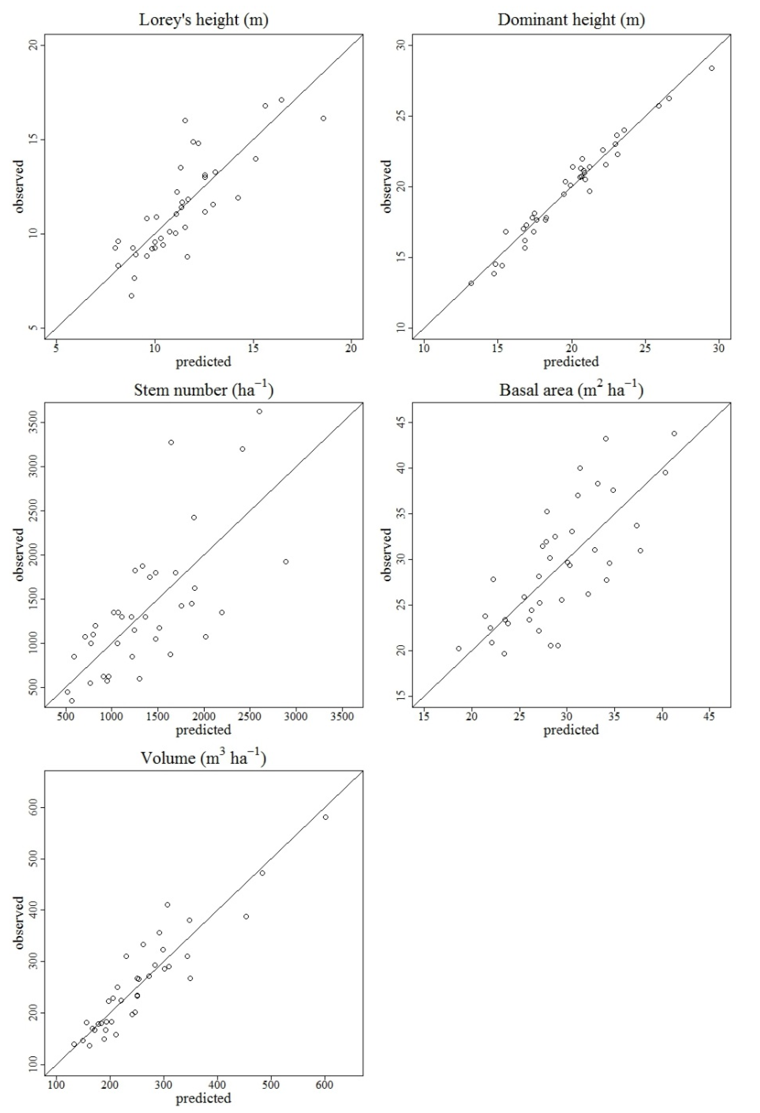
- Assess the accuracy of Lore’s mean height (hL), hdom, stem number (N), basal area (G), and stem volume (V) determined with an ABA combining UAS-SfM and field data in a small forest property (200 ha) in Norway.
- Evaluate the importance of using spectral information in modeling the abovementioned properties.
2. Study Area and Materials
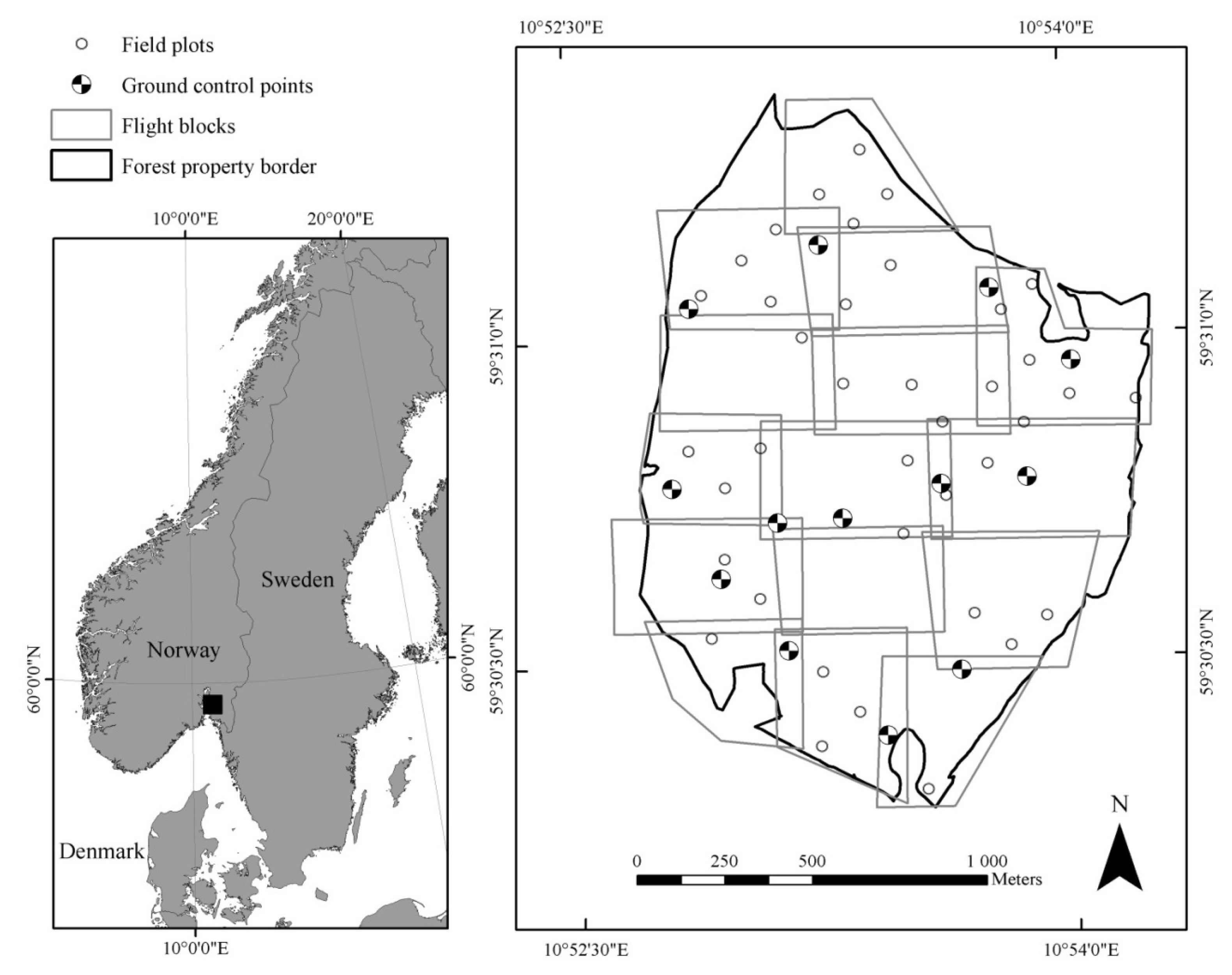
2.1. Study Area
2.2. Field Measurements


| Property | Range | Mean |
|---|---|---|
| hL (m) | 6.7–17.1 | 11.4 |
| hdom (m) | 13.1–28.4 | 19.8 |
| N (n∙ha−1) | 350.0–3625 | 1372 |
| G (m2∙ha−1) | 19.7–43.8 | 29.2 |
| V (m3∙ha−1) | 136.6–580.9 | 256.1 |
2.3. Remotely Sensed Data
3. Methods
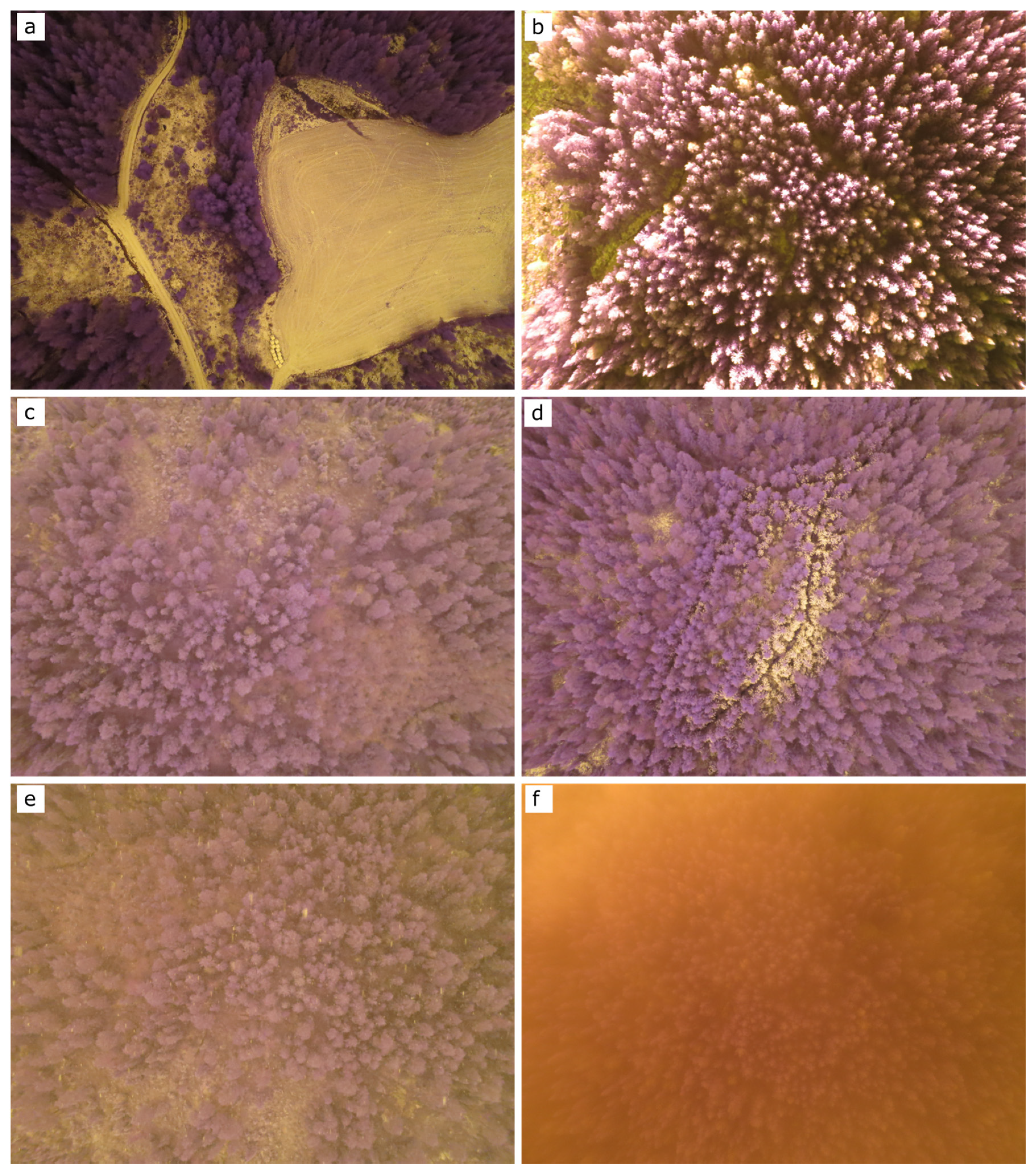
3.1. UAS Imagery Collection—Planning and Implementation

| Date | Flight#. | No. of Images | Flight Time (min) | Coverage (ha) | Size (MB) | Wind-Speed (m·sec−1) | Weather |
|---|---|---|---|---|---|---|---|
| 27.11.14 | 1 | 247 | 26 | 17.2 | 678 | 6–7 | Full cloud cover + snow |
| 29.11.14 | 2 | 223 | 24 | 19.7 | 734 | 4–5 | Full cloud cover |
| 3 | 252 | 27 | 17.5 | 832 | |||
| 4 | 197 | 23 | 14.6 | 654 | |||
| 5 | 186 | 23 | 15.7 | 613 | |||
| 30.11.14 | 6 | 194 | 23 | 14.4 | 636 | 4–5 | Full cloud cover |
| 7 | 226 | 25 | 14.2 | 742 | |||
| 8 | 227 | 25 | 17.1 | 775 | |||
| 9 | 237 | 26 | 17.2 | 825 | |||
| 02.12.14 | 10 | 220 | 24 | 18.2 | 686 | 3–5 | Full cloud cover + snow |
| 11 | 223 | 24 | 17.3 | 677 | |||
| 12 | 231 | 25 | 16.4 | 774 | |||
| 13 | 184 | 21 | 12.5 | 613 | |||
| 03.12.14 | 14 | 218 | 24 | 17.6 | 526 | 2–5 | Fog |
| 15 | 185 | 21 | 13.1 | 711 | Sun | ||
| TOTAL | 15 | 3250 | 361 | 242.7 | 10476 |
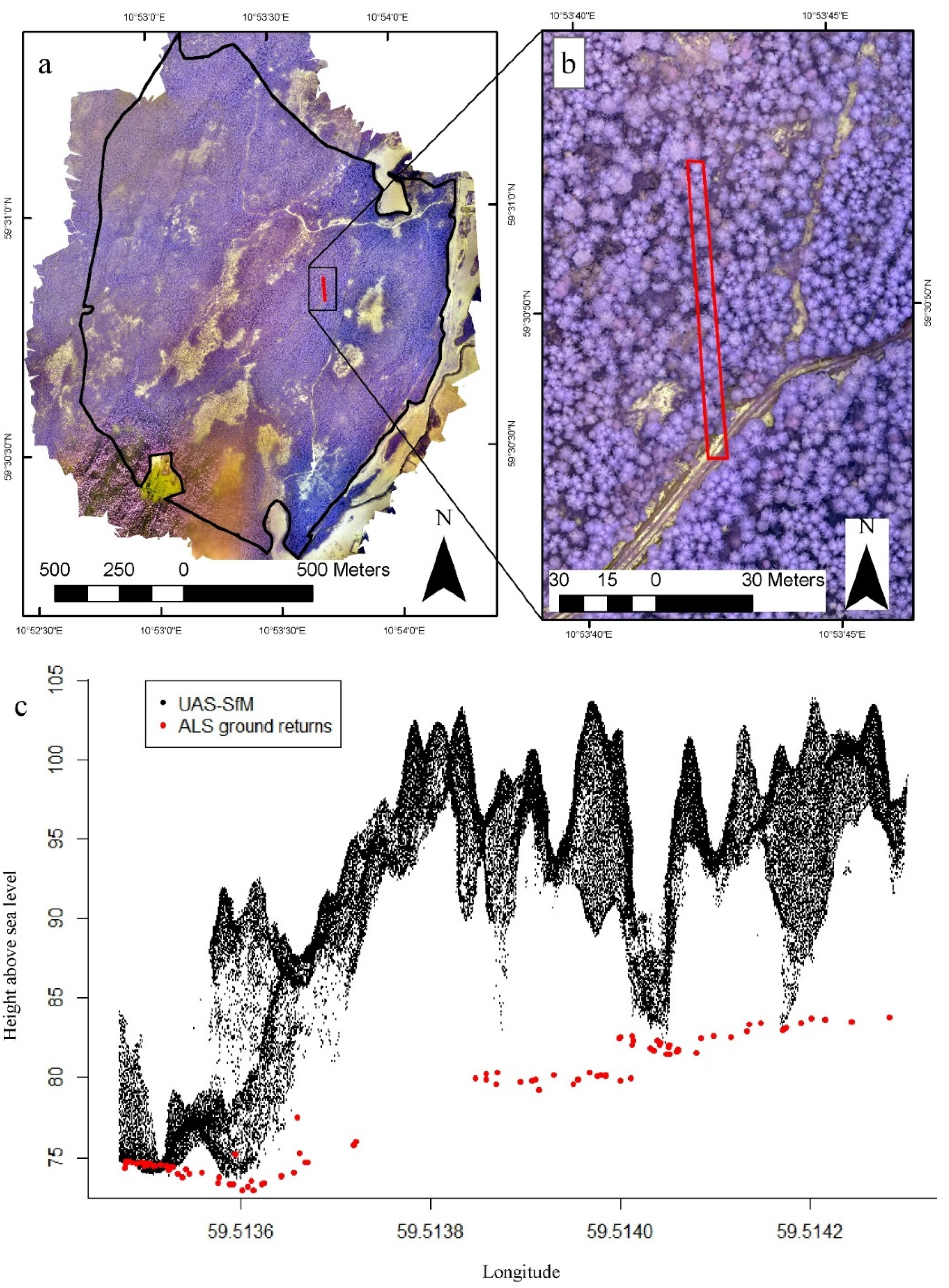
3.2. Photogrammetric Processing
| Task | Parameter |
|---|---|
| Align photos | Accuracy: high b |
| Pair selection: reference b | |
| Key point limit: 40000 b | |
| Tie point limit: 1000 b | |
| Build mesh | Surface type: height field b |
| Source data: sparse point cloud b | |
| Facecount: low (13544) a | |
| Interpolation: enabled b | |
| Guided marker positioning | |
| Optimize camera alignment | Marker accuracy (m): 0.005 b Projection accuracy (pix): 0.1 b Tie point accuracy (pix): 4 b Fit all except for k4 b Number of GCPs: 13 a |
| Build dense cloud | Quality: Medium a |
| Depth filtering: mild a |

3.3. Variable Extraction and Statistical Methods
4. Results
4.1. Regression Modeling
| Dependent Variable | Predictive Model a | Adj. R2 b | RMSE b | Relative RMSE b | b | Relative b |
|---|---|---|---|---|---|---|
| ln(hL) | p30 + hsd | 0.68 | 1.55 | 13.66 | 0.01 | 0.13 |
| ln(hL) | p20 + hsd + Gm | 0.71 | 1.51 | 13.28 | 0.00 | 0.03 |
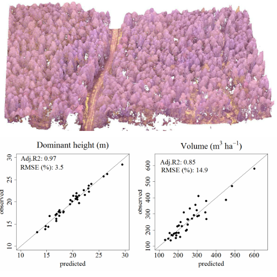
| hdom | p50 + hsd + d7 | 0.96 | 0.72 | 3.64 | 0.01 | 0.05 |
| hdom | p50 + hsd + d7 + Gm | 0.97 | 0.69 | 3.48 | 0.01 | 0.04 |
| ln(N) | p30 + d0 + d9 | 0.57 | 529.03 | 38.57 | -8.28 | -0.60 |
| ln(N) | p30 + d0 + d9 + Gsd | 0.60 | 538.31 | 39.24 | -4.90 | -0.36 |
| G | p100 + d0 + d9 | 0.60 | 4.49 | 15.38 | 0.03 | 0.09 |
| ln(V) | p80 + d0 | 0.85 | 38.30 | 14.95 | 0.54 | 0.21 |
4.2. Plot-Level Validation

5. Discussion
5.1. UAS-SfM Forest Inventory Accuracy
5.2. Importance of Spectral Variables
5.3. General Considerations
6. Conclusions
Acknowledgments
Author Contributions
Conflicts of Interest
References
- Wallace, L.; Lucieer, A.; Watson, C.; Turner, D. Development of a UAV-LiDAR system with application to forest inventory. Remote Sens. 2012, 4, 1519–1543. [Google Scholar] [CrossRef]
- Whitehead, K.; Hugenholtz, C.H. Remote sensing of the environment with small unmanned aircraft systems (UASs), part 1: A review of progress and challenges. J. Unmanned Veh. Syst. 2014, 2, 69–85. [Google Scholar] [CrossRef]
- Andersen, H.E.; Reutebuch, S.E.; McGaughey, R.J. A rigorous assessment of tree height measurements obtained using airborne lidar and conventional field methods. Can. J. Remote Sens. 2006, 32, 355–366. [Google Scholar] [CrossRef]
- Lisein, J.; Pierrot-Deseilligny, M.; Bonnet, S.; Lejeune, P. A photogrammetric workflow for the creation of a forest canopy height model from small unmanned aerial system imagery. Forests 2013, 4, 922–944. [Google Scholar] [CrossRef]
- Whitehead, K.; Hugenholtz, C.H.; Myshak, S.; Brown, O.; LeClair, A.; Tamminga, A.; Barchyn, T.E.; Moorman, B.; Eaton, B. Remote sensing of the environment with small unmanned aircraft systems (UASs), part 2: Scientific and commercial applications. J. Unmanned Veh. Syst. 2014, 2, 86–102. [Google Scholar] [CrossRef]
- Paneque-Gálvez, J.; McCall, M.; Napoletano, B.; Wich, S.; Koh, L. Small drones for community-based forest monitoring: An assessment of their feasibility and potential in tropical areas. Forests 2014, 5, 1481–1507. [Google Scholar] [CrossRef]
- Nex, F.; Remondino, F. UAV for 3D mapping applications: A review. Appl. Geomat. 2014, 6, 1–15. [Google Scholar] [CrossRef]
- Salamí, E.; Barrado, C.; Pastor, E. UAV flight experiments applied to the remote sensing of vegetated areas. Remote Sens. 2014, 6, 11051–11081. [Google Scholar] [CrossRef] [Green Version]
- Dandois, J.P.; Ellis, E.C. High spatial resolution three-dimensional mapping of vegetation spectral dynamics using computer vision. Remote Sens. Environ. 2013, 136, 259–276. [Google Scholar] [CrossRef]
- Hugenholtz, C.H.; Moorman, B.J.; Riddell, K.; Whitehead, K. Small unmanned aircraft systems for remote sensing and earth science research. Eos. Trans. Am. Geophys. Union 2012, 93, 236. [Google Scholar] [CrossRef]
- Watts, A.C.; Ambrosia, V.G.; Hinkley, E.A. Unmanned aircraft systems in remote sensing and scientific research: Classification and considerations of use. Remote Sens. 2012, 4, 1671–1692. [Google Scholar] [CrossRef]
- Næsset, E. Airborne laser scanning as a method in operational forest inventory: Status of accuracy assessments accomplished in Scandinavia. Scand. J. For. Res. 2007, 22, 433–442. [Google Scholar] [CrossRef]
- Vauhkonen, J.; Maltamo, M.; McRoberts, R.E.; Næsset, E. Introduction to forestry applications of airborne laser scanning. In Forestry Applications of Airborne Laser Scanning; Maltamo, M., Næsset, E., Vauhkonen, J., Eds.; Springer: Dordrecht, The Netherlands, 2014; pp. 1–16. [Google Scholar]
- Wallace, L.; Musk, R.; Lucieer, A. An assessment of the repeatability of automatic forest inventory metrics derived from UAV-Borne laser scanning data. IEEE Trans Geosci. Remote Sens. 2014, 52, 7160–7169. [Google Scholar] [CrossRef]
- Jaakkola, A.; Hyyppä, J.; Kukko, A.; Yu, X.; Kaartinen, H.; Lehtomäki, M.; Lin, Y. A low-cost multi-sensoral mobile mapping system and its feasibility for tree measurements. ISPRS J. Photogramm. Remote Sens. 2010, 65, 514–522. [Google Scholar] [CrossRef]
- Wallace, L.; Lucieer, A.; Watson, C.S. Evaluating tree detection and segmentation routines on very high resolution UAV LiDAR data. IEEE Trans Geosci. Remote Sens. 2014, 52, 7619–7628. [Google Scholar] [CrossRef]
- Wallace, L.; Watson, C.; Lucieer, A. Detecting pruning of individual stems using airborne laser scanning data captured from an unmanned aerial vehicle. Int. J. Appl. Earth Obs. Geoinf. 2014, 30, 76–85. [Google Scholar] [CrossRef]
- Chisholm, R.A.; Cui, J.; Lum, S.K.Y.; Chen, B.M. UAV LiDAR for below-canopy forest surveys. J. Unmanned Veh. Sys. 2013, 1, 61–68. [Google Scholar] [CrossRef]
- Aber, J.S.; Sobieski, R.J.; Distler, D.A.; Nowak, M.C. Kite aerial photography for environmental site investigations in Kansas. Trans. Kansas Acad. Sci. 1999, 102, 57–67. [Google Scholar] [CrossRef]
- Dunford, R.; Michel, K.; Gagnage, M.; Piégay, H.; Trémelo, M.L. Potential and constraints of unmanned aerial vehicle technology for the characterization of Mediterranean riparian forest. Int. J. Remote Sens. 2009, 30, 4915–4935. [Google Scholar] [CrossRef]
- Dandois, J.P.; Ellis, E.C. Remote sensing of vegetation structure using computer vision. Remote Sens. 2010, 2, 1157–1176. [Google Scholar] [CrossRef]
- Colomina, I.; Molina, P. Unmanned aerial systems for photogrammetry and remote sensing: A review. ISPRS J. Photogramm. Remote Sens. 2014, 92, 79–97. [Google Scholar] [CrossRef]
- Wang, T.; Yan, L.; Mooney, P. Dense point cloud extraction from UAV captured images in forest area. In Proceedings of the 2011 IEEE International Conference on Spatial Data Mining and Geographical Knowledge Services (ICSDM), Fuzhou, China, 29 June–1 July 2011.
- Gini, R.; Passoni, D.; Pinto, L.; Sona, G. Aerial images from an UAV system: 3D modeling and tree species classification in a park area. Int. Arch. Photogramm. Remote Sens. Spatial Inf. Sci. 2012, 39, 361–366. [Google Scholar] [CrossRef]
- Fritz, A.; Kattenborn, T.; Koch, B. UAV-based photogrammetric point clouds—Tree stem mapping in open stands in comparison to terrestrial laser scanner point clouds. Int. Arch. Photogramm. Remote Sens. Spat. Inf. Sci. 2013, 40, 141–146. [Google Scholar] [CrossRef]
- Imagine Games Network. MICMAC Software for Automatic Mapping in Geographical Context. Available online: http://logiciels.ign.fr/?Micmac (accessed on 7 March 2015).
- Trimble. Trimble Unmanned Aircraft Systems for Surveying and Mapping. Available online: http://uas.trimble.com/sites/default/files/downloads/trimble_uas_brochure_english.pdf (accessed on 7 March 2015).
- Packalen, P.; Strunk, J.; Mehtätalo, L.; Maltamo, M. Resolution Dependence in an area-based approach to forest inventory with ALS. Available online: http://ocs.agr.unifi.it/index.php/forestsat2014/ForestSAT2014/paper/view/387 (accessed on 15 June 2015).
- Sperlich, M.; Kattenborn, T.; Koch, B. Potential of Unmanned Aerial Vehicle Based Photogrammetric Point Clouds for Automatic Single Tree Detection. Available onlilne: http://www.dgpf.de/neu/Proc2014/proceedings/papers/Beitrag270.pdf (accessed on 15 January 2015).
- Bohlin, J.; Wallerman, J.; Fransson, J.E.S. Forest variable estimation using photogrammetric matching of digital aerial images in combination with a high-resolution DEM. Scand. J. For. Res. 2012, 27, 692–699. [Google Scholar] [CrossRef]
- Gobakken, T.; Bollandsås, O.M.; Næsset, E. Comparing biophysical forest characteristics estimated from photogrammetric matching of aerial images and airborne laser scanning data. Scand. J. For. Res. 2014, 30, 1–37. [Google Scholar] [CrossRef]
- Daamen, W. Results from a Check on Data Collection of the National Forest Survey in 1973–1977; Umeå: Institutionen för skogstaxering, Sveriges lantbruksuniversitet: Uppsala, Sweden, 1980; p. 189. (in Swedish) [Google Scholar]
- Eriksson, H. On Measuring Errors in Tree Height Determination with Different Altimeters; Stockholm Skogshögskolan, Institutionen för skogsproduktion: Stockholm, Sweden, 1970. (in Swedish) [Google Scholar]
- Fitje, A.; Vestjordet, E. Stand height curves and new tariff tables for Norway spruce. Commun. Nor. For. Res. Inst. 1977, 34, 23–62. [Google Scholar]
- Vestjordet, E. Merchantable volume of Norway spruce and Scots pine based on relative height and diameter at breast height or 2.5 m above stump level. Medd. Det Nor. Skogforsøksves. 1968, 25, 411–459. (in Norwegian). [Google Scholar]
- Braastad, H. Volume tables for birch. Medd. Nor. SkogforsVes 1966, 21, 23–78. (in Norwegian). [Google Scholar]
- Brantseg, A. Volume functions and tables for Scots pine. South Norway. Medd. Nor. SkogforsVes 1967, 22, 689–739. (in Norwegian). [Google Scholar]
- Vestjordet, E. Functions and tables for volume of standing trees. Norway spruce. Medd. Nor. SkogforsVes 1967, 22, 539–574. (in Norwegian). [Google Scholar]
- Terrasolid. TerraScan User’ s Guide. Available online: http://www.terrasolid.com/download/tscan.pdf (accessed on 17 July 2015).
- SenseFly. eBee Extended User Manual. Available online: https://www.sensefly.com/fileadmin/user_upload/documents/manuals/Extended_User_Manual_eBee_and_eBee_Ag_v16.pdf (accessed on 20 April 2015).
- SenseFly. User Manual S110 RGB/NIR/RE Camera. Available online: https://www.sensefly.com/fileadmin/user_upload/documents/manuals/user_manual_s110_v3.pdf (accessed on 15 November 2014).
- SenseFly. eMotion: Release Notes. Available online: https://www.sensefly.com/fileadmin/user_upload/documents/release_notes/Release_Notes_2.4.5.pdf (accessed on 15 April 2015).
- Quantum GIS Geographic Information System. Open Source Geospatial Foundation Project. Available online: http://www.qgis.org/it/site/ (accessed on 1 September 2014).
- Etterprosessering med Pinnacle. Available online: http://www.blinken.no/gnss-program.htm (accessed on 15 April 2015).
- Agisoft. Agisoft Photoscan User Manual. Available online: http://www.agisoft.com/pdf/photoscan-pro_1_1_en.pdf (accessed on 6 February 2015).
- Verhoeven, G.; Doneus, M.; Briese, C.; Vermeulen, F. Mapping by matching: a computer vision-based approach to fast and accurate georeferencing of archaeological aerial photographs. J. Archaeol. Sci. 2012, 39, 2060–2070. [Google Scholar] [CrossRef]
- Agisoft. Tutorial (Beginner level): Orthophoto and DEM Generation with Agisoft PhotoScan Pro 1.1 (with Ground Control Points). Available online: http://www.agisoft.com/pdf/PS_1.1%20-Tutorial%20(BL)%20-%20Orthophoto,%20DEM%20(with%20GCP).pdf (accessed on 6 February 2015).
- Yu, B.; Member, S.; Ostland, I.M.; Gong, P.; Pu, R. Penalized discriminant analysis of in situ hyperspectral data for conifer species recognition. IEEE Trans. Geosci. Remote Sens. 1999, 35, 2569–2577. [Google Scholar] [CrossRef]
- Wu, C. Normalized spectral mixture analysis for monitoring urban composition using ETM+ imagery. Remote Sens. Environ. 2004, 93, 480–492. [Google Scholar] [CrossRef]
- Dalponte, M.; Orka, H.O.; Gobakken, T.; Gianelle, D.; Næsset, E. Tree species classification in boreal forests with hyperspectral data. IEEE Trans Geosci. Remote Sens. 2013, 51, 2632–2645. [Google Scholar] [CrossRef]
- Dalponte, M.; Ørka, H.O.; Ene, L.T.; Gobakken, T.; Næsset, E. Tree crown delineation and tree species classification in boreal forests using hyperspectral and ALS data. Remote Sens. Environ. 2014, 140, 306–317. [Google Scholar] [CrossRef]
- Næsset, E. Practical large-scale forest stand inventory using a small-footprint airborne scanning laser. Scand. J. For. Res. 2004, 19, 164–179. [Google Scholar] [CrossRef]
- Nilsson, M. Estimation of tree heights and stand volume using an airborne lidar system. Remote Sens. Environ. 1996, 56, 1–7. [Google Scholar] [CrossRef]
- Næsset, E. Predicting forest stand characteristics with airborne scanning laser using a practical two-stage procedure and field data. Remote Sens. Environ. 2002, 80, 88–99. [Google Scholar] [CrossRef]
- Lumley, T.; Miller, A. Package “Leaps”: Regression Subset Selection. Available online: http://cran.r-project.org/web/packages/leaps/leaps.pdf (accessed on 2 June 2014).
- Snowdon, P. A ratio estimator for bias correction in logarithmic regressions. Canad. J. For. Res. 1991, 21, 720–724. [Google Scholar] [CrossRef]
- Gobakken, T.; Næsset, E. Estimation of diameter and basal area distributions in coniferous forest by means of airborne laser scanner data. Scand. J. For. Res. 2004, 19, 529–542. [Google Scholar] [CrossRef]
- Hakala, T.; Suomalainen, J.; Peltoniemi, J.I. Acquisition of bidirectional reflectance factor dataset using a micro unmanned aerial vehicle and a consumer camera. Remote Sens. 2010, 2, 819–832. [Google Scholar] [CrossRef]
© 2015 by the authors; licensee MDPI, Basel, Switzerland. This article is an open access article distributed under the terms and conditions of the Creative Commons Attribution license (http://creativecommons.org/licenses/by/4.0/).
Share and Cite
Puliti, S.; Ørka, H.O.; Gobakken, T.; Næsset, E. Inventory of Small Forest Areas Using an Unmanned Aerial System. Remote Sens. 2015, 7, 9632-9654. https://doi.org/10.3390/rs70809632
Puliti S, Ørka HO, Gobakken T, Næsset E. Inventory of Small Forest Areas Using an Unmanned Aerial System. Remote Sensing. 2015; 7(8):9632-9654. https://doi.org/10.3390/rs70809632
Chicago/Turabian StylePuliti, Stefano, Hans Ole Ørka, Terje Gobakken, and Erik Næsset. 2015. "Inventory of Small Forest Areas Using an Unmanned Aerial System" Remote Sensing 7, no. 8: 9632-9654. https://doi.org/10.3390/rs70809632