Article

An Automated Approach for Mapping Persistent Ice and Snow Cover over High Latitude Regions

by
David J. Selkowitz
1,2,* and
Richard R. Forster
2
1
U.S. Geological Survey, Alaska Science Center, 4210 University Drive, Anchorage, AK 99508, USA
2
Department of Geography, University of Utah, 260 S. Central Campus Dr., Room 270, Salt Lake City, UT 84112, USA
*
Author to whom correspondence should be addressed.
Remote Sens. 2016, 8(1), 16; https://doi.org/10.3390/rs8010016
Submission received: 30 June 2015 / Revised: 4 December 2015 / Accepted: 21 December 2015 / Published: 25 December 2015
(This article belongs to the Special Issue Remote Sensing of Changing Northern High Latitude Ecosystems)

Abstract

:
We developed an automated approach for mapping persistent ice and snow cover (glaciers and perennial snowfields) from Landsat TM and ETM+ data across a variety of topography, glacier types, and climatic conditions at high latitudes (above ~65°N). Our approach exploits all available Landsat scenes acquired during the late summer (1 August–15 September) over a multi-year period and employs an automated cloud masking algorithm optimized for snow and ice covered mountainous environments. Pixels from individual Landsat scenes were classified as snow/ice covered or snow/ice free based on the Normalized Difference Snow Index (NDSI), and pixels consistently identified as snow/ice covered over a five-year period were classified as persistent ice and snow cover. The same NDSI and ratio of snow/ice-covered days to total days thresholds applied consistently across eight study regions resulted in persistent ice and snow cover maps that agreed closely in most areas with glacier area mapped for the Randolph Glacier Inventory (RGI), with a mean accuracy (agreement with the RGI) of 0.96, a mean precision (user’s accuracy of the snow/ice cover class) of 0.92, a mean recall (producer’s accuracy of the snow/ice cover class) of 0.86, and a mean F-score (a measure that considers both precision and recall) of 0.88. We also compared results from our approach to glacier area mapped from high spatial resolution imagery at four study regions and found similar results. Accuracy was lowest in regions with substantial areas of debris-covered glacier ice, suggesting that manual editing would still be required in these regions to achieve reasonable results. The similarity of our results to those from the RGI as well as glacier area mapped from high spatial resolution imagery suggests it should be possible to apply this approach across large regions to produce updated 30-m resolution maps of persistent ice and snow cover. In the short term, automated PISC maps can be used to rapidly identify areas where substantial changes in glacier area have occurred since the most recent conventional glacier inventories, highlighting areas where updated inventories are most urgently needed. From a longer term perspective, the automated production of PISC maps represents an important step toward fully automated glacier extent monitoring using Landsat or similar sensors.

Graphical Abstract

1. Introduction

Glaciers have been identified as one of the most sensitive indicators of changes in climate [1,2] and have been identified as an essential climate variable that should be monitored globally [3]. Glaciers not only respond to changes in climate, but can also drive changes in the earth climate system through changes in albedo and contribution to sea level rise [4,5,6,7]. From a more local to regional perspective, glaciers often serve as a crucial source of runoff for downstream populations [8] and can present a potential hazard due to glacier lake outburst floods [9,10].
While the presence of exposed ice at the end of the melt season allows most glaciers to be positively identified under the right conditions, smaller glaciers cannot always be reliably distinguished from perennial snow cover patches. The challenge of discriminating between perennial snow cover patches and glaciers is confounded by the lack of satellite imagery acquired under ideal conditions when the maximum amount of ice is exposed. Consequently, even high quality glacier inventories created by image analysts may include some large perennial snow cover patches or omit some small glaciers. Image analysts are able to use contextual information (such as topographic position, patch shape, or ice or snow texture) to assist in discriminating between perennial snow cover patches and glaciers. Here we present a relatively simple automated approach designed to map glaciers that is likely to include a larger amount of perennial and consistently late lying seasonal snow cover patches than would be included in more traditional approaches. Therefore, although our intent is ultimately to map glaciers, we refer to the automated maps produced by the approach we describe as persistent ice and snow cover (PISC) maps, acknowledging that some perennial snow cover and late lying seasonal snow cover may be included.
Despite the important role of glaciers in the global earth system, in situ monitoring efforts are limited to a tiny fraction of the areas containing glaciers [11]. While field measurements of mass balance are irreplaceable indicators of the status of specific glaciers, spaceborne remote sensing can provide crucial complementary information such as the areal extent of ice cover over large regions encompassing numerous glaciers. For this reason, remote sensing approaches have been implemented as a key component of the tiered global glacier monitoring strategy for the Global Terrestrial Network for Glaciers (GTN-G) [12]. Optical remote sensing using the visible through middle infrared bands has been the method of choice for the majority of remote sensing efforts attempting to map glaciers. This is due to both the widespread availability of optical remote sensing data from sensors such as those from the Landsat series and the Advanced Spaceborne Thermal Emission and Reflection Radiometer (ASTER) as well as the relatively unique spectral signature of snow and ice cover in the optical remote sensing wavelengths.
Landsat image data have been used for a wide variety of glacier monitoring applications for more than 30 years. Early work with Landsat MultiSpectral Scanner (MSS) and Landsat Thematic Mapper (TM) focused on identification of glacier zones and calculation of corresponding reflectance values [13,14,15,16,17,18]. This was soon followed by glacier area mapping as well as change detection for areas covered by a single Landsat path-row [19,20,21]. Since the launch of the Landsat Enhanced Thematic Mapper Plus (ETM+) in 1999, numerous studies have used either the TM or ETM+ sensors (or in some cases, both sensors) to create glacier maps for increasingly large areas [22,23,24,25,26], with data from many of these studies included in the Global Land Ice Measurements from Space (GLIMS) database [27,28]. Even more recently, the Randolph Glacier Inventory (RGI) was compiled to be the first comprehensive glacier database with global coverage [29].
Despite the potential offered by remote sensing, comprehensive, fully inclusive glacier monitoring at spatial resolutions fine enough to detect changes in glacier area that typically occur over a decade or less has remained elusive in some regions. While global monitoring efforts such as GLIMS and more recently the RGI have been effective for mapping glaciers across many large regions, global coverage has only been achieved very recently and the glacier inventory dates within the global database span several decades. In addition, for many regions, mapping of changes in glacier area over time has not been conducted.
One reason why such large area inventories have not been completed more regularly or for more regions is because existing approaches have required a substantial time investment by skilled image analysts. While previous work has demonstrated that automated classification results are typically as good or better than manually digitized results [30], even automated mapping approaches still require investment of an analyst’s time in the pre-processing stage (selection and acquisition of appropriate scenes with minimal cloud cover and minimal seasonal snow cover) as well as the post-processing stage (manual editing to correct classification errors, add areas of debris-covered glacier ice, and remove areas of perennial and seasonal snow cover, sea ice and icebergs) [31]. In many cases, input from an image analyst is also necessary to determine appropriate thresholds for band ratios or individual bands during the main processing stage. Manual correction of automatically-derived drainage divides from digital elevation models can also be a time consuming part of the process in some cases.
We demonstrate that, across the circumpolar Arctic, and perhaps globally, the extent of PISC can be regularly monitored using fully automated processing of Landsat data that exploits all available cloud-free, shadow-free data available from the late summer period. This approach represents an important step toward fully automated monitoring of glacier extent across large regions. In addition, PISC maps generated by this approach can also be used to rapidly identify areas where substantial changes may have occurred since the most recent conventional glacier inventories were conducted and thus highlight areas where updated glacier inventories are most urgently needed. Finally, many applications can potentially benefit from regularly updated PISC maps, including land surface models, runoff models, and general circulation models (GCMs).

2. Study Regions

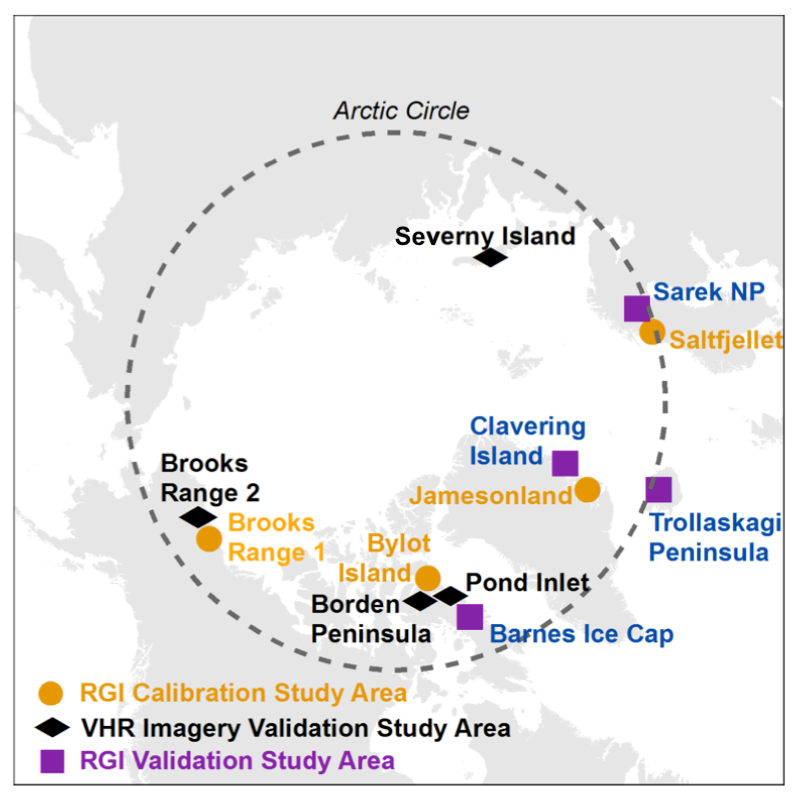
We developed and tested the automated PISC mapping approach using data from four regions distributed throughout the Arctic, which we refer to as RGI calibration study areas (Figure 1, Table 1). Each RGI calibration study area covered a 35 × 35 km area, with glaciers covering as much as 66% of the study domain at Bylot Island, Canada and as little as 11% of the study domain in the Brooks Range in the United States (as indicated by the RGI dataset). We tested the PISC mapping algorithm at four additional 35 × 35 km study areas, referred to as RGI validation study areas, as well as at four smaller (approximately 15 × 15 km) study areas where we acquired very high resolution imagery (VHRI) (Figure 1, Table 1), referred to as VHRI validation study areas. The selection of 35 × 35 km bounding regions for the RGI calibration and RGI validation study areas was constrained to areas within the RGI database above 65°N with >5% ice cover where the dates of imagery used to construct the RGI glacier inventory were known to be within a single year. Allowing for these constraints, we selected 35 × 35 km study areas to represent a range of glacier types, topography, and climatic conditions. The selection of VHRI validation study areas was constrained to areas above 65°N with >5% ice cover where acceptable very high resolution imagery from the period 2010–2015 was available from the DigitalGlobe archive of data from the WorldView 2 or WorldView 3 satellites (mention of a particular product does not constitute endorsement by the U.S. federal government). To be considered acceptable for our purposes, very high resolution imagery needed to contain a contiguous area of ~15 × 15 km or larger with >5% ice cover that was cloud-free and nearly or completely free of late lying seasonal snow cover from the previous winter as well as nearly or completely free of recently accumulated snowfall. Allowing for these constraints, as with the selection of RGI calibration and RGI validation study areas, we selected study areas intended to represent a range of glacier types, topography, and climate conditions. Two of the four VHRI validation study areas were 15 × 15 km in size, while the others were 16 × 14 km and 17.5 × 12.9 km due to cloud cover.
Table 1. Study area locations and characteristics.
Study AreaCountryTypeVHRI SensorLatLonIce CoverWRS-2 Path/Row
Brooks Range 1USARGI calibrationn/a69.3°N144.0°W11%68/11, 69/12, 70/11, 71/11, 72/11
SaltfjelletNorwayRGI calibrationn/a66.7°N14.2°E26%197/13, 198/13, 199/13, 200/13
Bylot IslandCanadaRGI calibrationn/a73.4°N79.0°W66%30/8, 31/8, 32/8, 33/8, 34/8, 35/8
JamesonlandGreenlandRGI calibrationn/a71.8°N25.0°W61%226/9, 226/10, 227/9, 228/9, 229/9, 230/9, 231/9
Clavering IslandGreenlandRGI validationn/a74.3°N21.0°W20%227/8, 228/7, 228/8, 229/7, 230/7, 231/7
Barnes Ice CapCanadaRGI validationn/a69.6°N72.0°W47%22/11, 23/11, 24/11, 25/11
Trollaskagi PeninsulaIcelandRGI validationn/a65.7°N18.8°W8%218/14, 219/14, 220/14
Sarek NPSwedenRGI validationn/a67.3°N17.7°E10%196/13, 197/13, 198/13
Brooks Range 2USAVHRI validationWorldView 269.2°N144.8°W6%69/11, 70/11, 71/11, 72/11
Borden PeninsulaCanadaVHRI validationWorldView 273.3°N82.7°W47%33/8, 34/8, 35/8, 36/8
Pond InletCanadaVHRI validationWorldView 372.3°N75.7°W83%27/9, 28/9, 29/9, 30/9
Sverny IslandRussiaVHRI validationWorldView 274.3°N55.7°E34%177/8, 178/7, 178/8, 179/7, 180/7
Figure 1. Study area locations across the circumpolar Arctic.
Remotesensing 08 00016 g001

3. Data

3.1. Landsat Data

Most land areas on the surface of the Earth are imaged by each active Landsat sensor every 16 days, resulting in 22 or 23 potential scenes each year that cover a specific area of interest. For most regions outside of the conterminous United States, however, only a limited selection of scenes imaged by the Landsat TM and ETM+ instruments have been downloaded and archived [32], resulting in the availability of far less than 22–23 scenes per year for many areas [33]. Finally, persistent cloud cover is an additional factor that further reduces the number of useful surface views. A typical glacier monitoring or mapping effort involves identifying cloud-free images (or portions of images), or for larger regions, collection of images, acquired during the seasonal minimum snow cover extent period. While in theory this is straightforward, the typically short duration of the snow-free period on and around glaciers does not always coincide with the availability of a cloud-free satellite acquisition. As a result, accurate glacier mapping requires careful scene selection by skilled analysts with knowledge of the region and the seasonal snow cover conditions during the period of interest. The analyst must select optimal scenes for automated or semi-automated glacier classification [30].
Overlapping Landsat paths result in more frequent image acquisitions for locations covered by more than 1 path. While only about 5% of the land surface is covered by multiple paths at the equator [34], at high latitudes, due to the convergence of Landsat paths, path overlap is ubiquitous, with many ground locations covered by three or more Landsat paths. This results in a doubling or even tripling of the number of Landsat scenes covering an area of interest. Assuming a substantial portion of these scenes have been acquired and archived (global scene availability is described in [33]), the odds of finding one or more scenes (or portions thereof) that capture the minimum annual extent of snow and ice under cloud-free conditions theoretically increases substantially with latitude. In our approach, we exploit this relative abundance of scenes available at many high latitude locations and consider all available Landsat TM or ETM+ data for each location, using an automated cloud classification algorithm to identify all instances of cloud-free views for each pixel location.
The majority of studies mapping glacier area using Landsat data have used uncorrected raw digital number (DN) or top-of-atmosphere (TOA) reflectance image data. Previous work has shown, however, that the use of atmospherically corrected surface reflectance image data can improve the accuracy of the results [35], and that atmospheric correction is particularly crucial if the Normalized Difference Snow Index (NDSI), which incorporates Landsat band 2 where atmospheric scattering is particularly high, is used [36]. To limit errors that could be introduced by variable atmospheric conditions when applying a standardized algorithm across large regions and over different dates, we make use of the atmospherically corrected USGS surface reflectance climate data record (CDR) product available for the Landsat TM and ETM+ sensors [37]. The surface reflectance CDR applies atmospheric correction routines originally developed for the Moderate Resolution Imaging Spectroradiometer (MODIS) to Landsat data. Surface reflectance is computed using the Second Simulation of a Satellite Signal in the Solar Spectrum (6S) radiative transfer model, which requires water vapor, ozone, geopotential height, aerosol optical thickness, and a digital elevation model along with Landsat TOA reflectance data. Application of 6S at high latitudes does violate the assumption of a plane-parallel atmosphere, which can impact the quality of surface reflectance product. However, because this is the standard atmospheric correction approach currently applied to all Landsat scenes and because we have not seen any evidence of errors large enough to affect the ability to discriminate between ice or snow and other surfaces in high latitude Landsat surface reflectance data, we have opted to use the standardized Landsat surface reflectance product.
For the RGI calibration and RGI validation study areas, we acquired and processed Landsat top-of-atmosphere (TOA) reflectance and surface reflectance products [36] from all available Landsat TM and ETM+ scenes available during the late summer (in this case defined as 1 August–15 September) for five-year periods. The TOA and surface reflectance Landsat scene products were produced by and acquired from the USGS EROS Data Center. We used the EarthExplorer interface to identify scenes acquired during the time period of interest at each of our study areas and then submitted orders for the identified scenes, subset to our study areas, using the EROS Science Processing Architecture (ESPA) interface. For the RGI calibration and RGI validation study areas, scenes were acquired for the five-year period centered on the date of the RGI inventory. At the Saltfjellet, Norway primary study area we acquired data from an additional year (for a total of six years) due to the poor availability of cloud-free scenes over the five-year period centered on the RGI mapping year. For the VHRI validation study areas, we acquired Landsat scenes for the 2010–2014 period, as the very high resolution imagery was acquired during 2014 or 2015.

3.2. Randolph Glacier Inventory Data

At each of the four RGI calibration study areas, we used glacier polygons provided by the RGI (version 4.0) to conduct sensitivity analysis for two key thresholds described below, as well as to conduct an accuracy assessment of mapped glacier area using our automated approach. The RGI provides polygon datasets of all glaciers in a region mapped using a variety of image resources, including Landat TM and ETM+ data. While the imagery source and mapping approach are not identified in the RGI database, the date or range of dates used to map each glacier are included in the database for most entries. Although some RGI polygons indicate a range of years and others provide no information about date or year of the image or other resource used for mapping, all RGI data used in this study indicated a specific date or range of dates within a single year covering the entire extent of each 35 × 35 km study area.

4. Methods

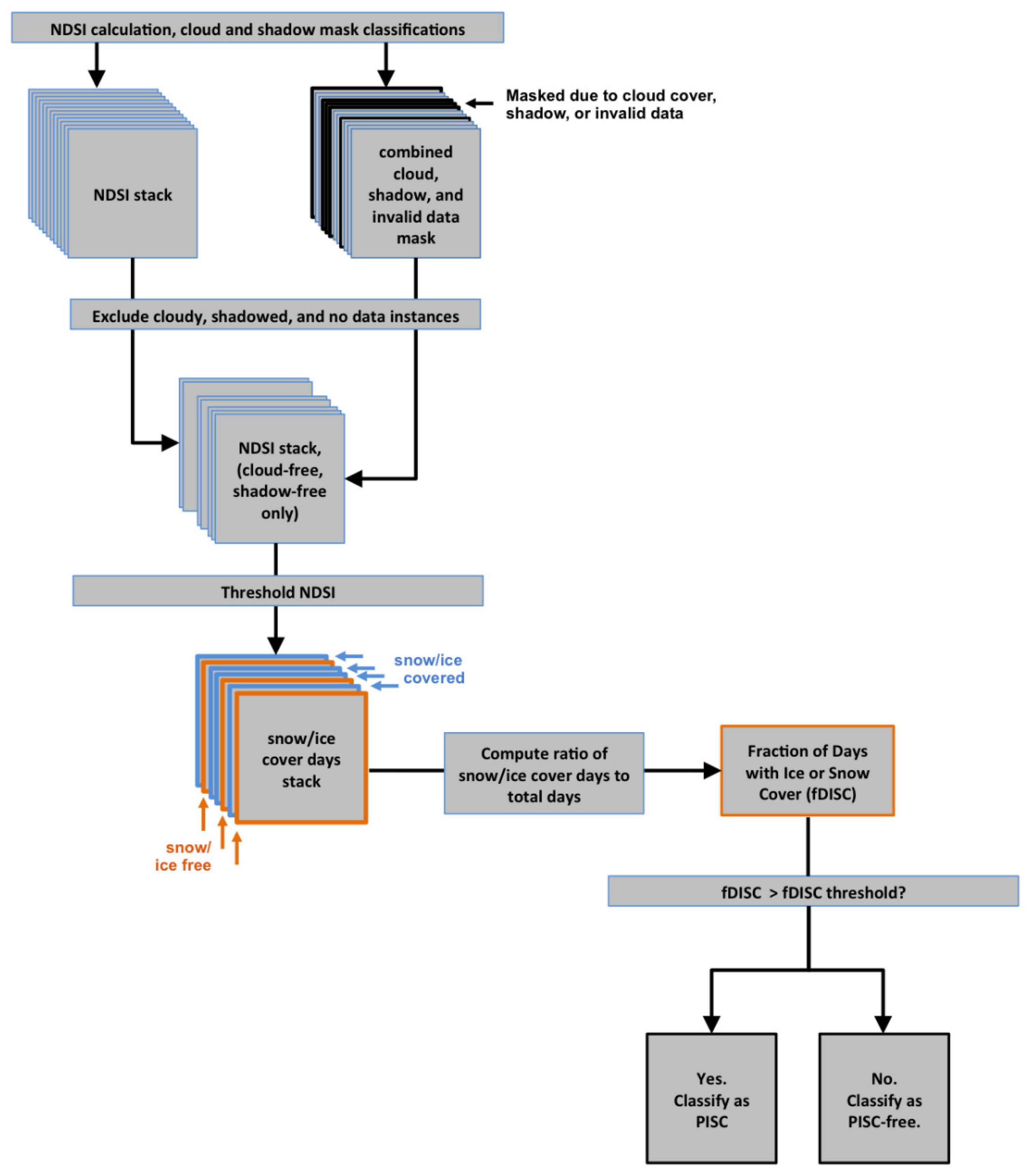
For each pixel in the study domain, our approach identifies the available cloud-free, shadow-free (and otherwise valid) land surface views and then compiles a stack of NDSI values corresponding to each valid land surface view. A threshold value is then applied to the stack of NDSI values to identify each land surface view in the stack as snow or ice-covered or snow or ice-free. The ratio of days with snow/ice to the total days, which we refer to as the fraction of Days with Ice or Snow Cover (fDISC) is then computed and a second threshold value is used to identify the pixel as PISC or PISC-free. A diagram of this processing flow is presented in Figure 2.
Figure 2. Diagram of processing flow for classification of Persistent Ice and Snow Cover (PISC) for a single pixel.
Remotesensing 08 00016 g002

4.1. Cloud and Shadow Masking

Analysis of stacks of numerous Landsat scenes requires an accurate automated cloud-masking approach. The CFmask algorithm [
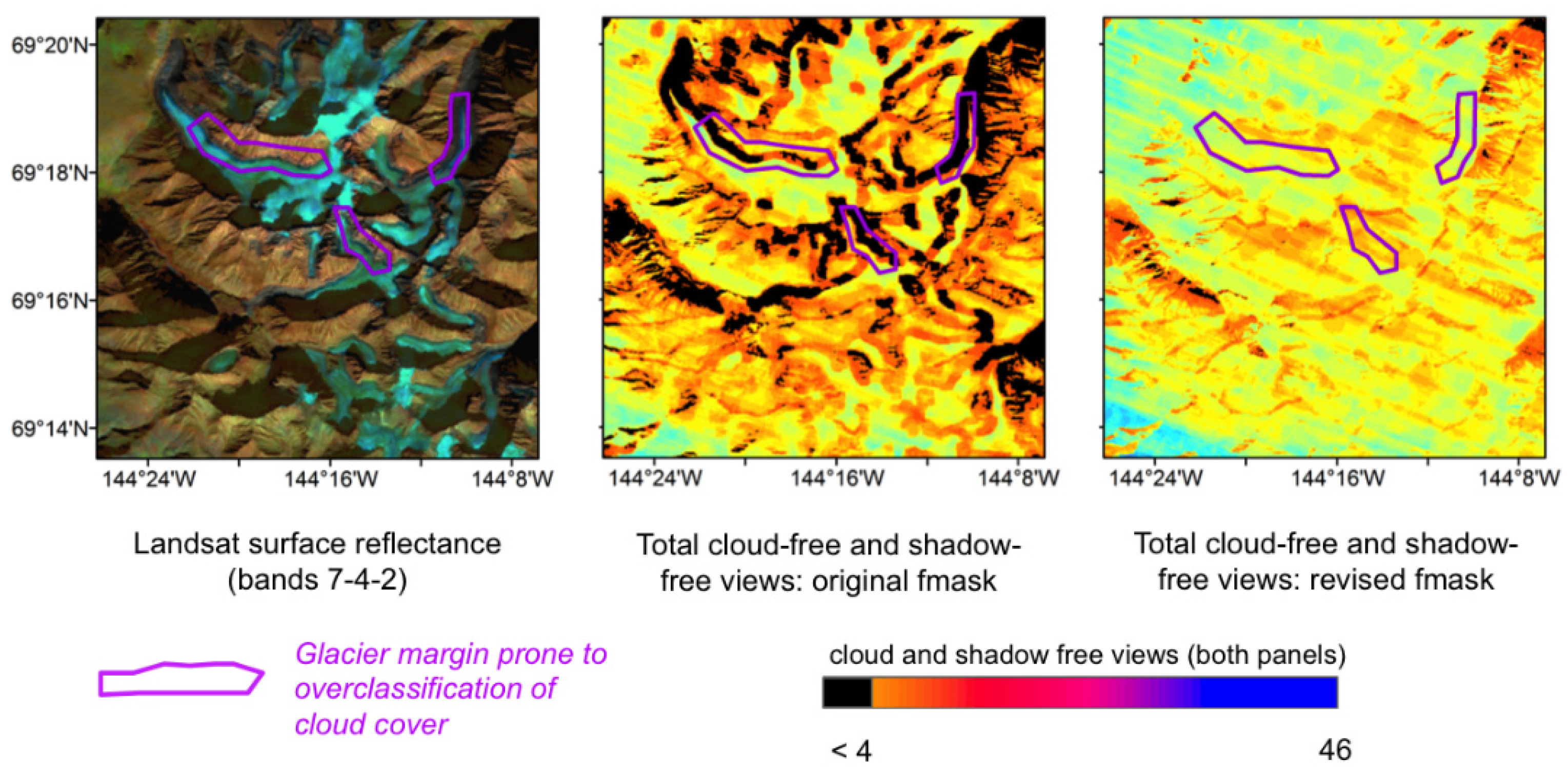
38] uses a series of rules based on cloud physical properties to develop a potential cloud layer from Landsat top-of-atmosphere reflectance data in bands 1–5 and 7 as well as brightness temperature from band 6. The potential cloud layer is then segmented to produce cloud objects, and ultimately a cloud mask and cloud-shadow mask that is provided with each USGS Climate Data Record (CDR) Landsat surface reflectance scene. While the overall accuracy of the CFmask cloud mask has been reported as 96.4%, our evaluation of CFmask cloud masks found that in rocky, alpine terrain and areas with a mixture of snow, ice, and other land cover types, the CFmask algorithm was prone to errors of commission (false positives) for cloud cover (an example is shown in Figure 3). More importantly, the errors of commission were not randomly distributed across areas with rock and ice cover, but were consistently present at the same patches of land cover on multiple occasions, thus resulting in a potential bias in available cloud-free data. We considered the high rate of errors of commission and particularly the potential for bias to be unacceptable for our purposes. We implemented a revised cloud masking approach designed to reduce errors of commission from the CFmask cloud masks over mountainous environments dominated by rock, snow, and ice, allowing us to fully exploit nearly all available cloud-free land surface views acquired during the late summer period. The revised cloud masking approach employed classification trees that reevaluated all instances of pixels where the CFmask product indicated cloud cover. The classification trees were originally developed for a seasonal snow covered area monitoring project and are based on over 100,000 pixels acquired from 20 Landsat scenes from mountainous areas across the globe. The classification tree approach relies on data from Landsat bands 1–5 and 7 to make a final distinction between cloud-covered and cloud-free pixels in cases where the original CFmask indicated cloud cover. Testing of the classification tree approach in conjunction with the original CFmask data indicated a slight improvement in overall accuracy (from 89% to 91%), with a major improvement in accuracy for high mountain areas from around the globe with substantial snow and ice cover (from 66% to 88%).
Figure 3. Comparison of original CFmask and revised CFmask for Bylot Island Landsat scene acquired 12 August 1999. (a) Landsat surface reflectance 7-4-2 band combination; (b) original CFmask cloud cover classification; and (c) revised CFmask cloud cover classification.
Remotesensing 08 00016 g003
In addition to cloud cover, both cloud shadows and terrain shadows can impact surface reflectance to the extent that band ratios such as the NDSI no longer provide a reliable indication of land surface characteristics. We excluded the most deeply shadowed pixels from further analysis by masking pixels where apparent surface reflectance in both bands 2 and 4 was <7%, as all land surface types in our region (with the exception of water) would be expected to exceed 7% reflectance in one or both of these bands. While our shadow masking approach was relatively unsophisticated and did not differentiate between cloud shadows and terrain shadows, we found it to be effective for our needs and ideal in that it required neither accurate cloud heights (for cloud shadow masking) nor accurate digital elevation model data (for terrain shadow masking).
All ETM+ scenes acquired after 2002 included missing data due to the failure of the Landsat 7 scan line corrector. Pixels that were not sampled due to the scan line corrector failure were identified and excluded from further analysis along with pixels identified as cloud-covered or shadowed.

4.2. Snow and Ice Mapping

For each late summer cloud-free, shadow-free view of the earth surface within our study areas, the normalized difference snow index (NDSI) [39,40] was used to discriminate between snow and ice free land and snow or ice cover. The NDSI typically exhibits positive values for partially and fully snow or ice covered land and negative values for most other land surface types. For the Landsat TM and ETM+ sensors, NDSI is defined by the following equation [39]:
NDSI = (TM2 − TM5)/(TM2 + TM5)
where TM2 is surface reflectance in Landsat TM or ETM+ band 2, and TM5 is surface reflectance in Landsat TM or ETM+ band 5. The Landsat TM and ETM+ sensors are prone to saturation in the visible bands, including band 2 used in the calculation of the NDSI, over bright surfaces such as snow and ice cover. This problem is more pronounced, however, at lower latitudes where higher levels of incoming solar radiation result in higher levels of reflected solar radiation over comparable surfaces. We calculated the incidence of saturation in band 2 for all scene subsets used in our study areas and found that saturation occurred in only 0.7% of cloud-free surface views.
While NDSI values close to 1.0 almost always indicate relatively fresh snow cover with high albedo and values <0 almost always indicate snow-free or ice-free land, the threshold used for identification of snow cover presence has varied considerably in previous applications, prompting us to undertake an uncertainty analysis, described in detail below. The most appropriate threshold value for discrimination between snow-covered and snow-free pixels depends on several factors, including contamination with dust or fine debris, snow grain size, illumination characteristics, as well as the minimum subpixel snow cover fraction for which positive identification of snow cover is desired.
In addition to an NDSI threshold used to discriminate between ice/snow cover and ice/snow-free land for each available cloud-free, shadow-free land surface view, it was also necessary to establish a threshold for the total fraction of late summer days with ice/snow cover above which a pixel is considered to be PISC (Figure 2). We refer to this second threshold as fDISC (fraction of Days with Ice or Snow Cover). If ice/snow cover could be identified with perfect accuracy, it would make sense to identify a pixel as PISC only if the selected NDSI threshold was exceeded in all available cloud-free and shadow-free land surface views. However, the lack of a well-established NDSI threshold as well as the occasional errors of omission in the cloud masking approach (resulting in the inclusion of cloud-covered pixels in the dataset of cloud-free and shadow-free pixel observations) complicated the situation. Due to these and potentially other complicating factors, we hypothesized that the optimum threshold for fDISC indicating PISC at a pixel would be lower than 1.0.
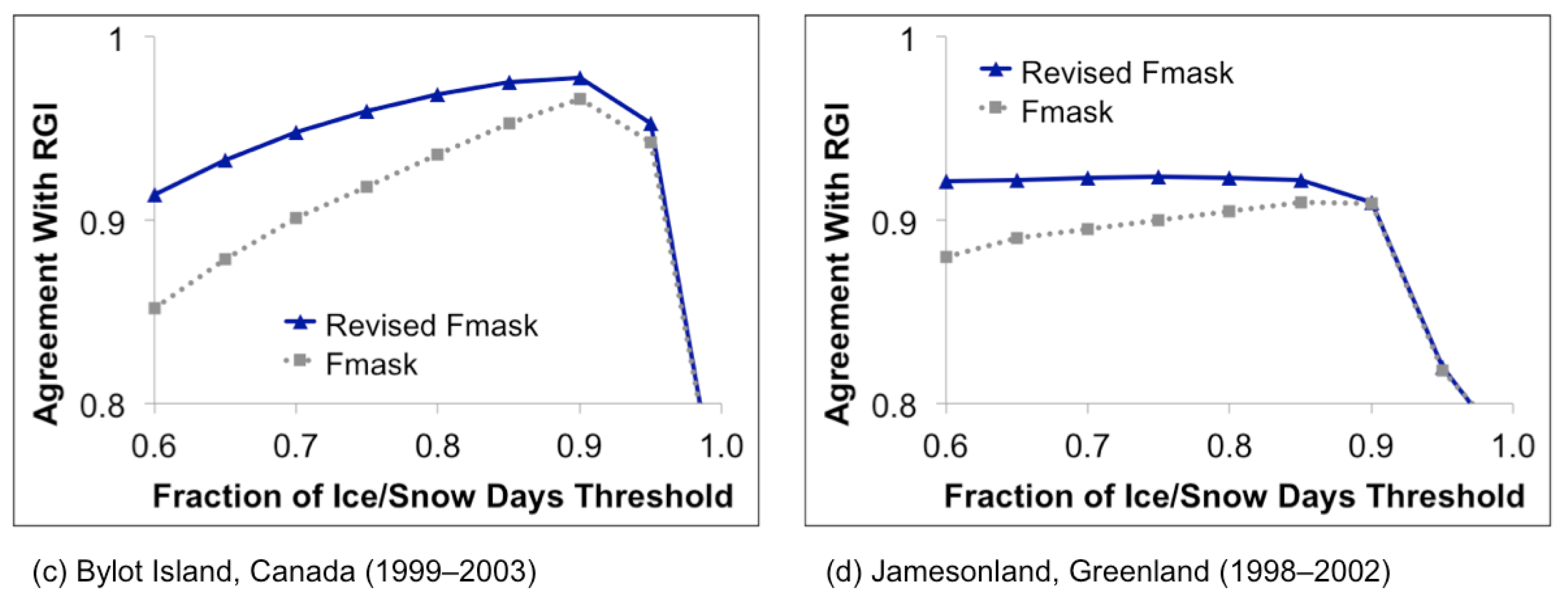
We addressed the uncertainty in optimum values for both the NDSI threshold and the fDISC threshold by conducting sensitivity analyses to determine the impact of variation in threshold values on classification results. For NDSI threshold values ranging from 0.2 to 0.5 (using increments of 0.1) and for fDISC threshold values ranging from 0.6 to 1.0 (using increments of 0.05), we computed PISC maps for each incremental value and compared the PISC maps to the RGI glacier outlines for the period, calculating the fraction of total pixels in agreement for each instance. Results of the sensitivity analysis, as well as the threshold value we selected for the final version of our algorithm are discussed in Section 5.

4.3. Additional Processing Steps

We reduced the number of cases where small perennial snow patches or very late lying seasonal snow patches were mapped as PISC by applying stricter standards for mapping PISC in smaller patches less than 300 pixels (27 ha) in size. This was accomplished by applying a sieve routine [41] at two different steps in the processing. The initial sieve routine was applied to identify patches mapped as PISC (based on an fDISC threshold of 0.8) <300 contiguous pixels (27 ha) in size. Pixels within these patches were then reclassified as snow/ice-free if they did not exceed the NDSI threshold in all available cloud-free, shadow-free Landsat surface views. Pixels located within larger patches of PISC (>300 contiguous pixels in size) were not subject to the stricter threshold and were mapped as PISC as long as they exceeded the NDSI threshold in at least 80% of cloud-free, shadow-free views. We also applied a second sieve routine to remove any mapped patches of PISC <100 pixels (9 ha) in size. While the implementation of the sieve routines did result in some errors of omission (false negatives) for small glaciers, it substantially reduced the error of commission and ensured that only the largest perennial snow cover patches were included in our inventory of PISC. Finally, to minimize speckle in the resulting classification, we implemented a post-processing 5 × 5 pixel median filter.

4.4. Accuracy Assessment

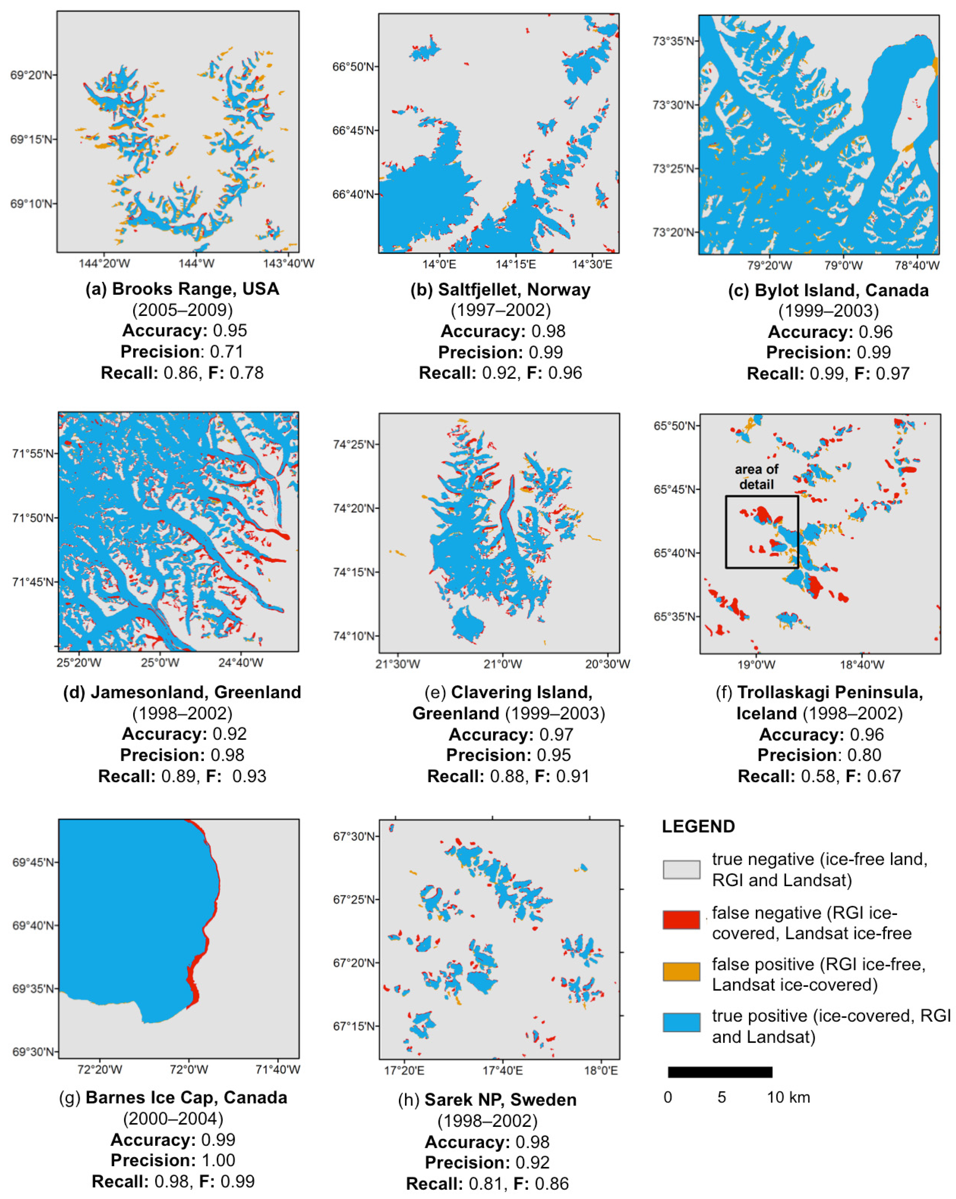
We assessed the accuracy of the resulting PISC maps at each study area by comparing PISC maps from our approach to the glacier outlines from the RGI. While the accuracy at the four RGI calibration study areas could potentially be biased because those study areas were used to identify optimal threshold values for NDSI and fDISC used in the algorithm, the four RGI validation study areas and the VHRI validation study areas were included to allow for an unbiased assessment at study areas that had not been used in the algorithm development.
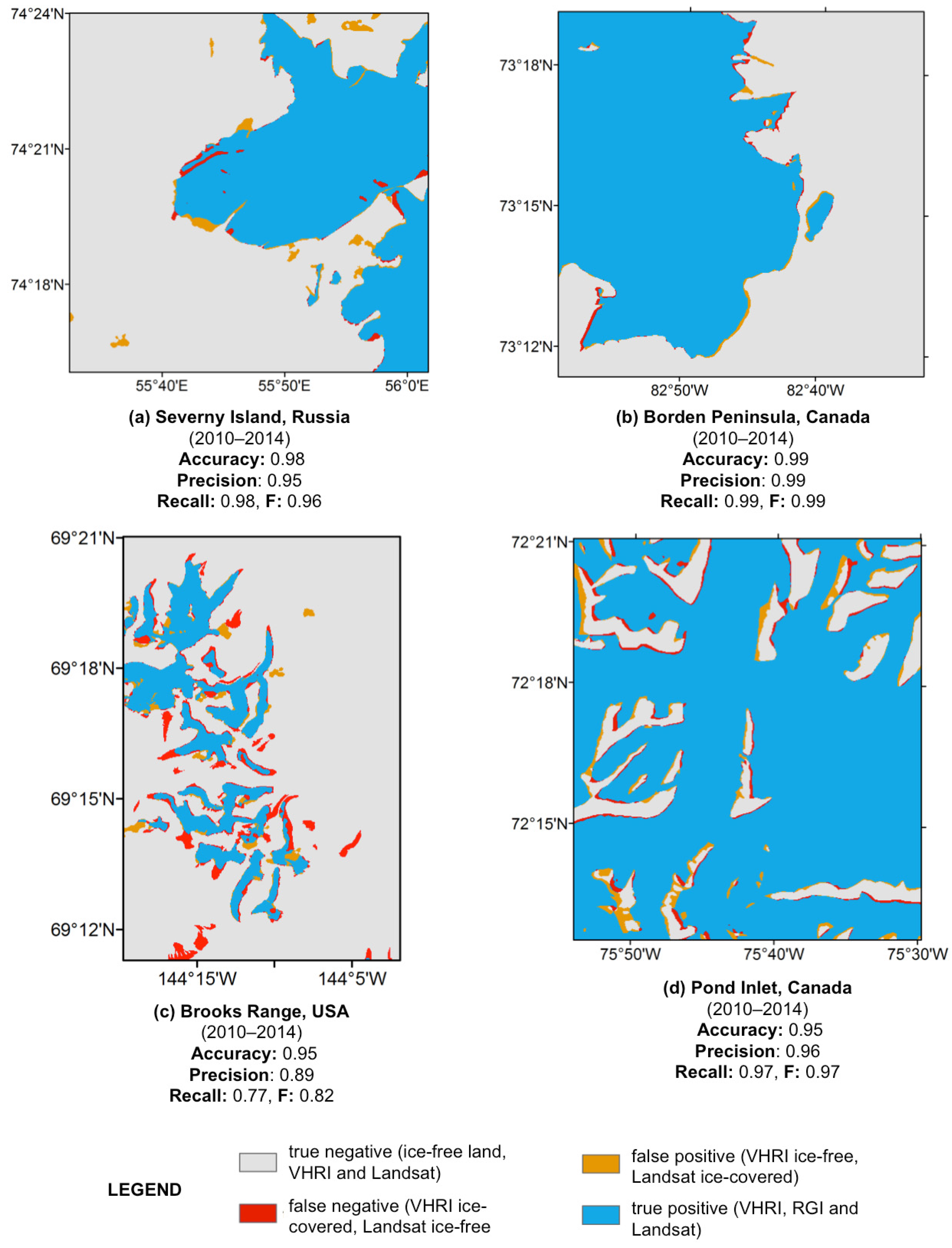
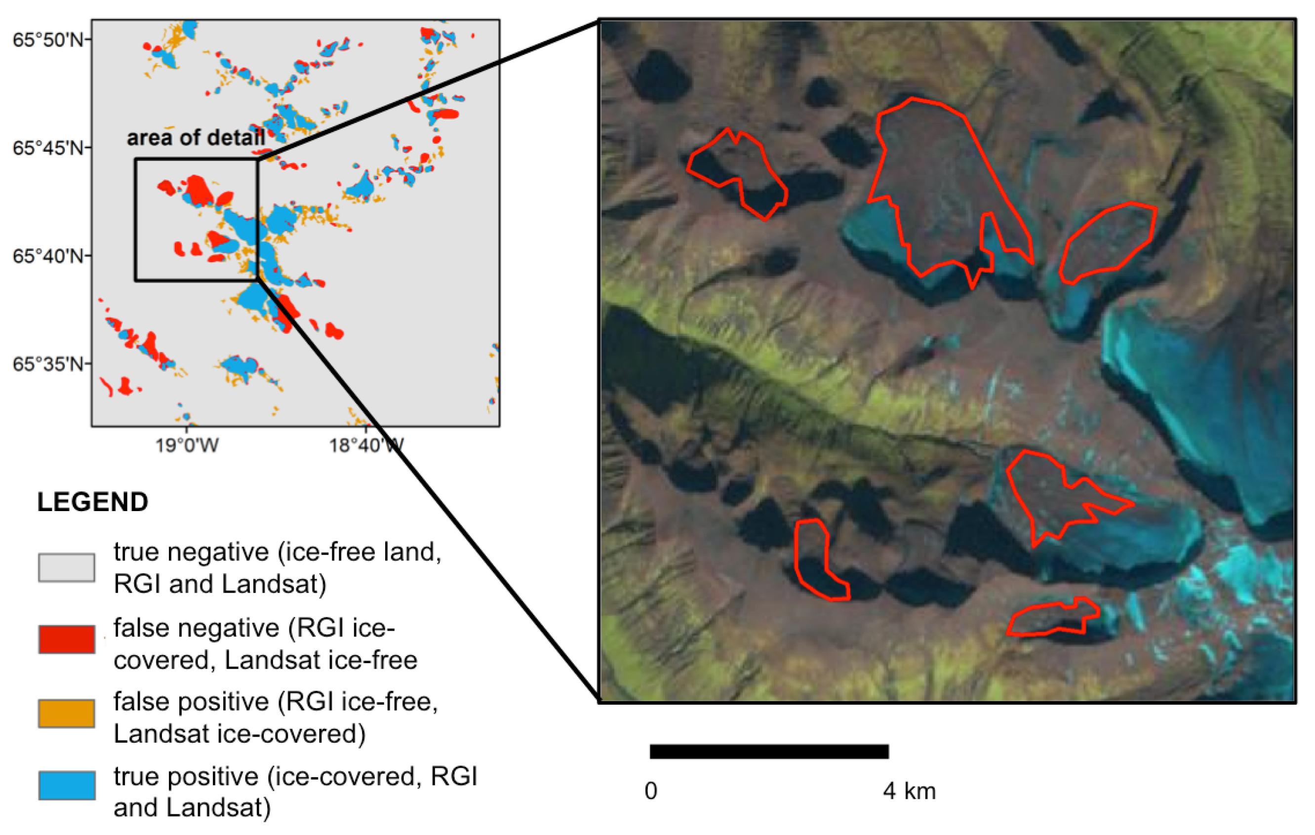
For each VHRI study area, an image analyst manually identified polygons of glacier ice. The set of polygons mapped as ice-covered were then converted to a binary 30-m raster dataset. The 30-m binary ice cover image was then compared to the PISC maps produced from the automated approach.
For the calculation of accuracy assessment metrics, we considered the RGI-derived or VHRI-derived glacier maps to be “truth” in the comparison with PISC maps computed using our approach. Using this assumption, we placed each pixel into one of four categories: (1) true positive (PISC mapped in both our approach and in the RGI or VHRI dataset); (2) false positive (PISC mapped in our approach, but ice-free land indicated by the RGI or VHRI dataset); (3) true negative (ice-free land mapped in both our approach and the RGI or VHRI dataset); and (4) false negative (ice free land mapped in our approach, but ice-cover mapped in the RGI or VHRI dataset). Based on these four categories, for each study area we calculated metrics commonly employed in assessment of binary snow and ice cover maps [42,43]: overall accuracy, precision (the user’s accuracy for the glacier and perennial snow cover class), recall (the producer’s accuracy for the glacier and perennial snow cover class), and F (a metric that incorporates both precision and recall). Accuracy, precision, recall, and F metrics were calculated using the following equations:
Accuracy = (TP + TN)/(TP + TN + FP + FN)
Precision = TP/(TP + FP)
Recall = TP/(TP + FN)
F = 2 TP/(2 TP + FP + FN)
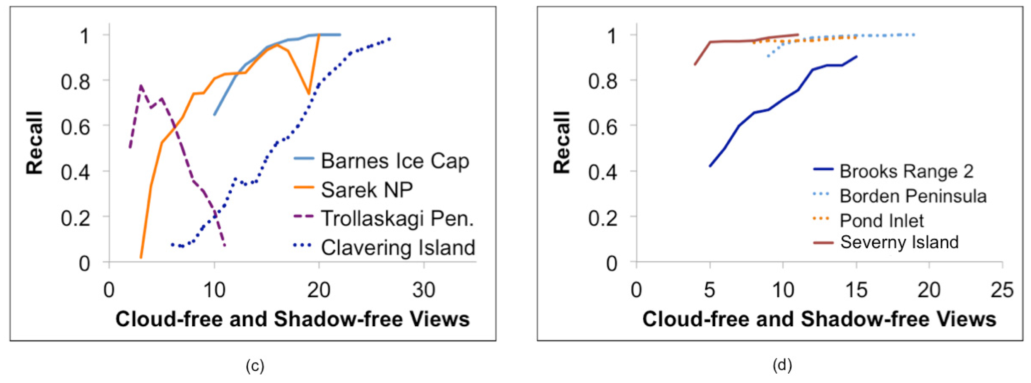
where TP is the number of true positive pixels, TN is the number of true negative pixels, FP is the number of false positive pixels, and FN is the number of false negative pixels. At each study area, we also calculated each assessment metric for all pixels with a given number of cloud-free and shadow-free land surface views to assess the impact of the number of observations on accuracy.

5. Results

5.1. Overall Accuracy

After considering the effect of the NDSI and fDISC thresholds on accuracy, discussed further below, we selected an NDSI threshold of 0.4 and fDISC threshold of 0.8. All results presented below use these threshold values (unless otherwise noted).
The mean overall accuracy for the primary and RGI validation datasets, defined here as agreement with the RGI validation dataset, was 0.964, while mean overall precision (user’s accuracy for the PISC class) was 0.918, mean overall recall (producer’s accuracy for the PISC class) was 0.863, and mean F was 0.883. The mean overall accuracy for the VHRI validation study areas was 0.968, while mean overall precision was 0.948, mean overall recall was 0.928, and mean overall F was 0.935. Accuracy, precision, and recall, as well as the spatial distribution of errors, are shown in Figure 4 for the RGI calibration and RGI validation study areas and in Figure 5 for the VHRI validation study areas.
Figure 4. Agreement with the Randolph Glacier Inventory (RGI) glacier extent for each full study area and validation study area. (a) Brooks Range, USA; (b) Saltfjellet, Norway; (c) Bylot Island, Canada; (d) Jamesonland, Greenland; (e) Clavering Island, Greenland; (f) Trollaskagi Peninsula, Iceland; (g) Barnes Ice Cap, Canada; (h) Sarek NP, Sweden.
Remotesensing 08 00016 g004
Figure 5. Agreement with VHRI-derived glacier extent for each VHRI validation study area. (a) Severny Island, Russia; (b) Borden Peninsula, Canada; (c) Brooks Range, USA; (d) Pond Inlet, Canada.
Remotesensing 08 00016 g005
While most Landsat-derived PISC maps closely resemble those from the RGI or from VHRI, we observed several notable differences. At the Trollaskagi Peninsula study area (Figure 4f), a substantial area mapped as ice-covered by the RGI was mapped as PISC-free by our technique. Closer examination of imagery data from this area, shown in Figure 6, indicated that most of the difference between glacier extent mapped by the RGI and PISC mapped by our technique was due to the RGI’s inclusion of substantial areas of debris-covered ice that is spectrally more similar to nearby ice-free land than to ice or snow cover. For the Brooks Range RGI calibration study area, our approach mapped numerous patches of PISC not mapped by the RGI (Figure 4a). Most of these false positive ice cover patches mapped by our technique were located in areas that were deeply shadowed by surrounding terrain during the latter part of our mapping period. As a result, our mapping approach was only able to consider data from the earlier part of the mapping period. Areas that become heavily shadowed later in the mapping period tend to receive lower levels of incoming solar radiation throughout the earlier part of the summer as well, and consequently often retain seasonal snow cover for all but a few weeks of the year. In many cases, this brief snow-free period does not begin until these areas have already become heavily shadowed, and consequently, there are no valid Landsat surface views of these areas after they have become snow free. Finally, at the Brooks Range VHRI validation study area, several small- and medium-sized glaciers identified by the RGI were not mapped as PISC. This is likely due to the strict requirement that patches of PISC smaller than 300 contiguous pixels be mapped as snow or ice covered in every cloud-free and shadow-free surface view. As a result, if NDSI dropped below 0.4 due to debris cover or cloud-contamination for any of the available cloud-free and shadow-free surface views, pixels part of these smaller patches of PISC were not mapped as PISC.
Figure 6. Agreement between mapped PISC and glaciers mapped with RGI for the Trollaskagi Peninsula, Iceland, with area of detail showing Landsat imagery and areas of false positives for PISC outlined in red.
Remotesensing 08 00016 g006

5.2. Factors Affecting Persistent Ice and Snow Cover Map Accuracy

5.2.1. Use of Original CFmask vs. Revised Cloud Masking Approach

The number of cloud-free and shadow-free land surface views available differed considerably depending on the cloud masking approach used, with substantially more views available for some pixels when the revised cloud masking approach, rather than the original CFmask cloud classification provided with the Landsat surface reflectance product, was used (Table 2, Figure 7). In addition, well-defined fine scale spatial patterns related to terrain and land cover type were apparent in the mapped total number of cloud-free and shadow-free views calculated using the original CFmask algorithm cloud masks, but not in the mapped total number of cloud-free and shadow-free views calculated using the revised cloud masking approach (Figure 7). While coarser scale patterns in the geographic distribution of cloud cover likely do exist, the well-defined fine scale patterns in the number of cloud-free views mapped by CFmask suggest a tendency to classify specific types of land cover and terrain as cloud-covered even in the absence of actual cloud cover (such as the example provided in Figure 3). While in some cases the mean number of cloud and shadow free surface views was not substantially different, at three of the four study areas, the percentage of pixels with <5 cloud-free and shadow-free surface views was substantially higher when the original CFmask was used for cloud identification (Table 2).
The reduced frequency of pixels with <5 cloud-free and shadow-free surface views for the revised cloud masking approach is not, in and of itself, an indication that the revised cloud masking approach is more effective, as this could simply indicate increased errors of omission for cloud cover. Analysis from previous work we conducted to assess the suitability of the standard CFmask product for seasonal snow cover monitoring applications does, however, indicate that in mountainous areas where fine scale mixtures of rock, snow, and ice are common, errors of commission (false positives) for cloud cover are widespread for the standard CFmask product. A different but equally useful way to compare the utility of the original and revised cloud masking approaches is to compare the accuracy (in this case, agreement with the RGI glacier extent) of mapped PISC using the original CFmask algorithm with the accuracy of mapped PISC using the revised cloud masking approach. This comparison indicated that in the majority of cases, the revised cloud masking approach yielded more accurate final results, and that at some study areas (particularly the Brooks Range), the improvement in accuracy was substantial (Figure 8).
Table 2. Comparison of cloud-free and shadow-free surface views (CFSFSV) for each study area using the original CFmask and the revised cloud masking approach.
Study AreaOriginal CFmaskRevised Approach
Mean CFSFSVPixels with <5 CFSFSVMean CFSFSVPixels with <5 CFSFSV
Brooks Range15.011.0%20.81.2%
Saltfjellet7.328.2%10.09.1%
Bylot Island29.40.0%29.50.0%
Jamesonland14.44.3%16.40.8%
Figure 7. Cloud-free and shadow-free views for a subset of the Brooks Range study area using the original CFmask and the revised cloud masking approach. Examples of glacier margins where false cloud cover was consistently identified, resulting in <4 cloud-free and shadow-free surface views are highlighted in purple.
Remotesensing 08 00016 g007
Figure 8. Accuracy (agreement with the RGI) for each study area as a function of late summer snow cover days threshold using the original CFmask and the revised cloud masking approach. (a) Brooks Range, USA; (b) Saltfjellet, Norway; (c) Bylot Island, Canada; (d) Jamesonland, Greenland.
Remotesensing 08 00016 g008aRemotesensing 08 00016 g008b

5.2.2. Normalized Difference Snow Index (NDSI) threshold

The NDSI threshold value used to distinguish between ice/snow covered and ice/snow free land for individual dates had a relatively small effect on accuracy in most instances, although the impact of NDSI threshold was often larger for cases well outside the optimum range of thresholds for fraction of late summer snow cover days (Figure 9). At the optimum fDISC threshold (between 0.7 and 0.95, depending on the study area), differences in accuracy associated with variable NDSI thresholds between 0.2 and 0.5 were minimal.
Figure 9. Effect of fraction of Days With Ice and Snow Cover (fDISC) threshold and Normalized Difference Snow Index (NDSI) threshold on PISC map accuracy (defined as agreement with RGI glacier area) for each RGI calibration study area. (a) Brooks Range, USA; (b) Saltfjellet, Norway; (c) Bylot Island, Canada; (d) Jamesonland, Greenland.
Remotesensing 08 00016 g009

5.2.3. Fraction of Days with Ice and Snow Cover (fDISC) Threshold

The fDISC threshold used to classify pixels as PISC had a larger impact on accuracy than the NDSI threshold (Figure 9). The optimal fDISC threshold value fell between 0.7 (for Saltjellet, Norway) and 0.95 (for the Brooks Range, USA). For the Brooks Range and Bylot Island study areas, agreement with the RGI increased steadily for threshold values above 0.6, peaked around 0.9, and then decreased (dramatically in the case of Bylot Island). For the Saltjellet, Norway, and Jamesonland, Greenland study areas, accuracy was quite stable for threshold values between 0.6 and 0.8, with a gradual decline in accuracy at higher threshold values.

5.2.4. Selection of Algorithm Threshold Values for NDSI fDISC

Based on the sensitivity analysis presented above, we selected an NDSI threshold value of 0.4 and an fDISC threshold value of 0.8. We selected the NDSI threshold of 0.4 because in all cases we analyzed, the 0.4 NDSI curve included the optimum accuracy value or fell only slightly below the optimum accuracy value. The wider variability in the value of the optimum fDISC threshold presented more of a challenge for selecting the ideal threshold for the algorithm that would be applied across all study areas. While a higher threshold between 0.9 and 0.95 worked best at the Bylot Island and Brooks Range study areas, a lower threshold around 0.7 resulted in the highest accuracy at the Saltfjellet, Norway, and Jamesonland, Greenland sites. To select the threshold with the highest accuracy across the greatest range of sites, we selected a threshold of 0.8, which had yielded accuracy above 0.9 for all four RGI calibration study areas.

5.2.5. Number of Cloud-Free and Shadow-Free Land Surface Views

In the majority of cases, both the precision and recall accuracy metrics increased as the number of cloud-free and shadow-free surface views increased (Figure 10), as we might intuitively expect. In addition, the rate of increase leveled off in almost all cases, although the number of cloud free views at which this plateau was reached varied substantially across sites, from as few as 4 cloud-free and shadow-free views to as many as 30 cloud-free and shadow-free views. The Trollaskagi Peninsula in Iceland presented an unusual exception, with the recall metric decreasing steadily as a function of number of cloud and shadow free views. The poor overall accuracy as well as the inverse relationship between cloud-free, shadow-free views and recall for the Trollaskagi Peninsula study area are likely due to large areas of debris-covered ice mapped in the RGI but not identified as PISC in our approach. In most cases, precision was low when <10 cloud-free and shadow-free surface views were available. The Barnes Ice Cap study area provided a notable exception, where high precision was observed regardless of the number of cloud-free, shadow-free surface views. Conversely, the recall metric was low at the Barnes Ice Cap Study Area for cases where <20 cloud-free and shadow-free surface views were available, although this did not have a large effect on overall accuracy at this study area since >20 cloud-free and shadow-free surface views were available at the vast majority of pixels.
Figure 10. Effect of number of cloud and shadow free views on precision (user’s accuracy for the ice covered class) and recall (producer’s accuracy for the ice-covered class) for RGI validation study areas and VHRI validation study areas. (a) Effect of the number cloud-free and shadow-free views on precision for the RGI validation study areas; (b) effect of the number of cloud-free and shadow-free views on precision for VHRI validation study areas; (c) effect of the number of cloud-free and shadow-free views on recall for the RGI validation study areas; and (d) effect of the number of cloud-free and shadow-free views on recall for VHRI validation study areas.
Remotesensing 08 00016 g010aRemotesensing 08 00016 g010b

5.3. Spatial Distribution of Errors

Figure 4 and Figure 5 depict the spatial distribution of errors of commission (false positives) and errors of omission (false negatives) for each of the twelve study areas. While the frequency, type, and distribution of errors varies by study area, some common patterns emerge. False negatives are often concentrated along the margins of glaciers, and particularly near the end of glacier tongues where heavy debris cover is present. False positives, on the other hand, are more frequently concentrated in patches that are not contiguous with larger glaciers, particularly in the Brooks Range RGI calibration study area, Brooks Range VHRI validation study area, and Severny Island VHRI validation study area. These small patches appear to be primarily patches of late lying or perennial snow cover. Late lying seasonal snow cover patches mapped as PISC appear to be most common in areas that experience deep shadowing during the latter part of the image acquisition period. As a result, valid surface views are only available for these locations during the earlier part of the image acquisition period, when these areas are still snow covered, and as a result they are classified as PISC.

6. Discussion

6.1. Effect of Fraction of Days with Ice/Snow Cover (fDISC) Threshold

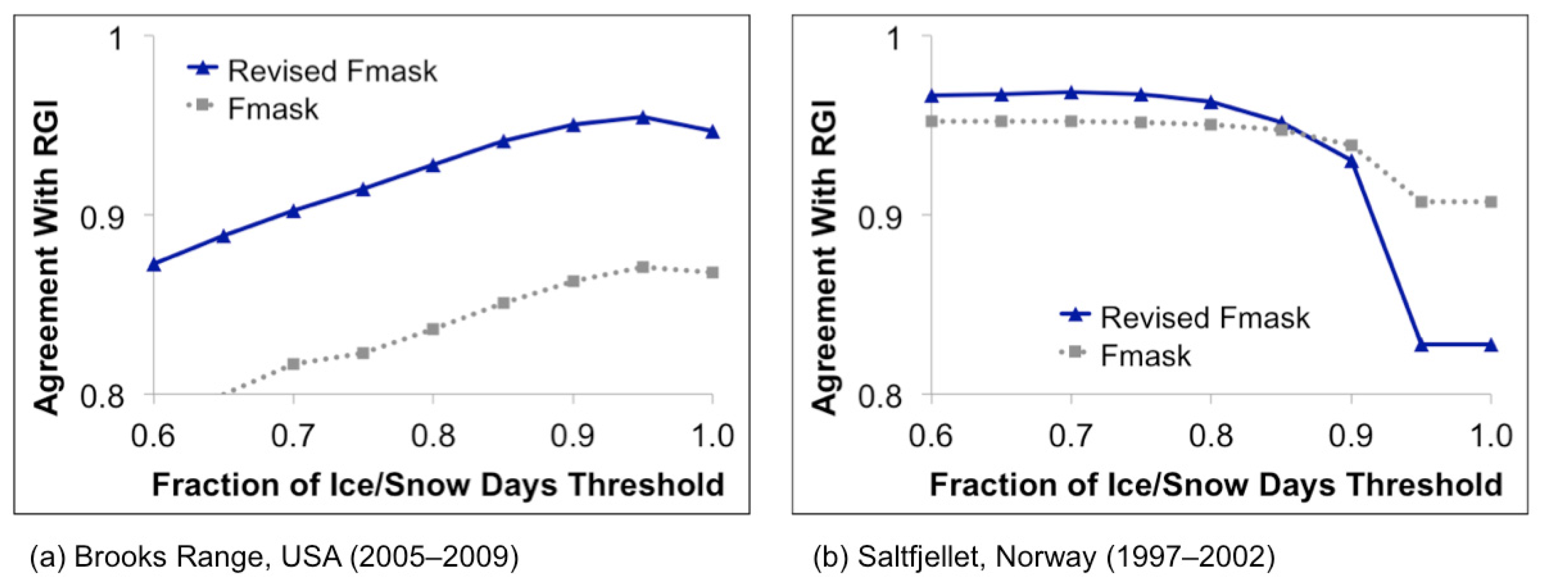
Our results suggest that a standardized approach where pixels with fDISC values >0.8 are classified as PISC should work well across much of the northern high latitude regions. However, the data also suggest that it may be possible to optimize the algorithm for specific regions by adjusting the fDISC threshold. The optimum value for this threshold will depend on a number of factors, including the prevalence of late lying seasonal snow patches in the region, the typical duration of seasonal snow cover, the prevalence of partially debris-covered ice on the lower portions of the glacier, and the number of cloud-free land surface views available.
Although we might intuitively expect a PISC mapping approach would perform best by mapping PISC only at pixels where all cloud-free and shadow-free views contained snow or ice cover, our results suggest this is not the case. While the optimum fDISC threshold value varies by study region, the optimum threshold is <1.0 for all study areas, and for the Bylot Island and Jamesonland study areas, accuracy drops off substantially as fDISC approaches 1.0. There are two primary reasons why the optimum threshold is consistently <1.0. First, because we know that the cloud mapping approach will occasionally classify cloud-contaminated pixels as cloud-free, we expect that cloud-contaminated observations of snow or ice cover will typically have lower NDSI values than cloud-free snow or ice and will often be mapped as free of snow and ice. Using a strict approach (equivalent to an fDISC threshold value of 1.0) would ensure that PISC pixels with even one cloud-contaminated view would be mapped as ice-free. Second, areas of PISC with debris cover will generally have NDSI values that decline over the course of the summer as more debris is exposed. While areas of PISC with partial debris cover will likely always maintain a positive NDSI value (as opposed to the majority of other land surface types, which will indicate negative NDSI values when snow-free), the NDSI value may briefly drop below the NDSI threshold (in this case 0.4), resulting in an occasional surface view that would be classified as free of snow and ice. Again, in these situations, using the strict approach with an fDISC threshold value of 1.0 would classify these pixels as ice-free.

6.2. Advantages and Disadvantages in Comparison to Traditional Semi-Automated Approaches

The automated PISC mapping approach presented here has both advantages and disadvantages when compared to more traditional approaches employed to produce the majority of existing glacier inventories. The primary advantage of the automated approach we present here is that it can be applied over large areas quickly, without the need for a substantial time investment from skilled analysts. This allows for generation of comprehensive PISC maps covering multiple time periods, allowing for analysis of changes in PISC extent over time. Prior to conducting this type of analysis, however, it will be necessary to develop techniques to distinguish between true changes in PISC and changes resulting in differences between the available data from different periods of comparison as well as changes in seasonal snow cover. With appropriate techniques for change analysis, we expect this type of approach could be used to map general trends in ice-covered area over time. Finally, the automated approach also ensures that results will be completely reproducible and not dependent on the level of expertise of a particular image analyst.
Perhaps the largest disadvantage of the automated approach is that it does not take into account contextual information, such as topographic position, patch size and shape, or snow or ice texture that an expert image analyst might be able to use to distinguish between glacier ice and perennial or late lying seasonal snow cover. To minimize the inclusion of perennial snow cover and late lying seasonal snow cover patches, we eliminate all patches mapped as PISC that are <100 contiguous pixels (~9 ha). While this minimum size threshold is somewhat larger than the thresholds typically used in more traditional glacier mapping approaches, we found that it substantially reduces the incidence of false positives while only slightly increasing the incidence of false negatives. Analysis of glaciers within our study areas indicates that, according to the RGI, glaciers <9 ha in size are entirely absent (or not mapped) in several of our study areas and account for only a tiny fraction of the total ice covered area where they are present, such as in the Brooks Range, where they account for just 0.6% of the ice covered area.
Another key disadvantage of the automated approach is that the mapped PISC cannot be tied to a single year, but instead maps PISC for a five-year period. This would become more important if the automated approach is implemented for the purpose of monitoring changes in PISC over time. In addition, the automated approach requires a number of late summer cloud-free views to be effective, while more traditional approaches where an image analyst carefully selects scenes for analysis can be effective if only a single, well-timed cloud-free scene is available. Finally, an image analyst can also typically identify large debris-covered glacier tongues, although delineating the exact extent of these features can be challenging even in cases where high resolution imagery is available [29]. In our automated mapping approach, partially debris-covered portions of glaciers may be mapped as PISC, particularly if seasonal snow cover is present for many of the late summer land surface views. Fully debris-covered portions of glaciers, however, will generally not be mapped as PISC. The difficulty of mapping debris-covered glacier ice has been a consistent problem for optical remote sensing efforts, and while several approaches have shown promise for automated mapping of debris-covered glacier ice [44,45,46], accurate mapping of debris-covered glacier ice will likely require some combination of manual editing or incorporation of other types of remotely sensed data.
Finally, it is important to note that conventional glacier inventories (such as those available from the RGI) identify and map individual glaciers, whereas our automated approach only identifies the extent of PISC. A single contiguous patch of ice cover mapped using our automated approach may represent two or more distinct glaciers separated by a drainage divide. Therefore, even in cases where the mapped extent of PISC corresponds perfectly with the extent of glacier ice, additional processing is necessary to generate outlines corresponding to individual glaciers. While in some cases this step can be accomplished with an automated approach, in certain cases (such as when the available DEM data is of poor quality), manual editing may be required.

6.3. Importance of Revised Cloud Masking Approach

The revised cloud masking approach implemented here appears to be crucial to the success of the overall approach, as the data indicate that using the original CFmask would result in substantial regions with <5 cloud-free and shadow-free observations due to frequent false positives for cloud cover over certain types of terrain and land cover. Most notably, many of these regions of consistent cloud cover commission errors are located along the margins of glaciers, which would result in a disproportionately large effect on the accuracy of the final product. This effect is confirmed by comparison of accuracy between versions of our approach implemented using the original CFmask classification and the revised cloud masking approach.

6.4. Application of the Approach to Lower Latitude Regions

A similar approach to the one presented here may be effective for mapping PISC in lower latitude regions. As the effective implementation of this approach relies on multiple cloud-free views during a relatively short window, we expect a similar approach would be most effective for lower latitude regions where cloudy days are relatively rare during the period when seasonal snow cover is at its minimum, as well as in regions where nearly all potential Landsat scenes have been archived (such as the conterminous U.S. and southern Canada). Application of this approach for lower latitude regions may also require adjustment of the seasonal window for Landsat scene inclusion. Finally, the relatively greater abundance of debris-covered glaciers at lower latitudes may present a problem given that the automated approach is not effective for mapping glaciers with extensive, optically thick debris cover.

6.5. Future Research

Future research should address the key disadvantages discussed above. In particular, it may be possible to compute various shape and texture metrics from the Landsat imagery as well as incorporate topographic information from a DEM and then use a machine learning approach to exploit some of the contextual information used by expert image analysts and improve classification accuracy. In addition, while we did not use any Landsat OLI data in our implementation of the automated approach because OLI data from only two late-summer periods had been acquired, Landsat OLI data offer several advantages that have the potential to improve classification accuracy. First, the higher radiometric range in the visible bands as well as the additional cirrus cloud detection band should allow for even more accurate cloud masking, resulting in fewer cloud-covered pixels being included in the analysis, as well as fewer cloud-free pixels omitted from the analysis. Second, the storage and transmission capacity of the Landsat 8 platform allows for collection of a greater number of scenes outside the conterminous United States, potentially allowing for shorter analysis windows (e.g., three years rather than five). While these improvements present the opportunity for more accurate monitoring of PISC, any efforts comparing PISC mapped with Landsat 5 (TM) or Landsat 7 (ETM+) instruments with PISC mapped with the Landsat 8 (OLI) instrument will need to carefully consider the potential impact of the differences in instrument specifications (particularly radiometric saturation in the visible bands) to ensure an unbiased analysis of change.
Unfortunately, the Landsat surface reflectance product was not optimized for atmospheric correction at higher latitudes. Because the plane parallel atmosphere assumption used in the 6S radiative transfer model is violated to some extent in our study region, the resulting surface reflectance data provided may be less accurate than similar data acquired at lower latitudes. The overall impact on mapping accuracy, however, is likely to be low, as our sensitivity analysis demonstrates that accuracy is much more impacted by the fDISC threshold than by the NDSI threshold. However, future improvements in the USGS surface reflectance CDR that improve accuracy at higher latitudes could potentially result in higher accuracy for our automated mapping approach.

7. Conclusions

We demonstrate the feasibility of accurate monitoring of debris-free PISC across the northern high latitudes using automated processing of Landsat TM and ETM+ data that does not require manual intervention from an image analyst at any point in the processing chain. This approach is made possible by the availability of a standardized Landsat surface reflectance product, the large number of scenes at high latitudes due to Landsat path overlap, and an enhancement to the standard Landsat surface reflectance cloud mask that reduces the occurrence of cloud cover false positives in mountainous, partially snow covered environments. Based on eight study areas distributed throughout the northern high latitudes, we found that results from our fully automated mapping approach are generally comparable to those obtained from the RGI at six of the eight RGI study areas. At the Trollaskagi, Iceland RGI validation site, agreement with the RGI glacier extent was very poor due to the substantial areas of debris-covered glaciers mapped by the RGI, while at the Brooks Range RGI calibration study area, agreement with the RGI database was lower than at most other sites due to the considerable amount of perennial and late lying seasonal snow cover mapped in areas indicated to be ice-free by the RGI. Our results agreed well with glacier maps derived from high resolution imagery at three of four validation sites, with lower accuracy at the Brooks Range site resulting from false negatives for portions of glaciers frequently in shadow and for portions of glaciers with substantial debris cover.
The approach presented here has the potential to quickly map PISC across large high latitude regions and provide important updates regarding the status of PISC, which can be particularly valuable when the resources to conduct more precise, traditional glacier monitoring efforts are not available.

Acknowledgments

Funding for this research was provided by the Land Remote Sensing Program of the US Geological Survey. We also wish to thank Daniel McGrath and four anonymous reviewers who provided substantial feedback for improving the manuscript.

Author Contributions

David J. Selkowitz developed the glacier mapping, validation, and cloud masking approaches. Richard R. Forster assisted with the development of the study design and interpretation of the results.

Conflicts of Interest

The authors declare no conflict of interest.

References

  1. Lemke, P.; Ren, J.; Alley, R.B.; Allison, I.; Carrasco, J.; Flato, G.; Fujii, Y.; Kaser, G.; Mote, P.; Thomas, R.H.; et al. Observations: Changes in snow, ice and frozen ground. In Climate Change 2007—The Physical Science Basis: Working Group I Contribution to the Fourth Assessment Report of the IPCC; Solomon, S., Qin, D., Manning, M., Chen, Z., Marquis, M., Averyt, K., Tignor, M., Miller, H.L., Jr., Eds.; Cambridge University Press: Cambridge, UK; New York, NY, USA, 2007; Chapter 4; pp. 337–384. [Google Scholar]
  2. Stocker, T.; Qin, D.; Plattner, G.-K.; Tignor, M.; Allen, S.K.; Boschung, J.; Nauels, A.; Xia, Y.; Bex, V.; Midgley, P.M. Climate Change 2013: The Physical Science Basis; Cambridge University Press: Cambridge, UK; New York, NY, USA, 2014. [Google Scholar]
  3. Sessa, R.; Dolman, H. Terrestrial Essential Climate Variables for Climate Change Assessment, Mitigation and Adaptation (GTOS 52); Food and Agriculture Organization of the United Nations: Rome, Italy, 2008. [Google Scholar]
  4. Fairbanks, R.G. A 17,000-year glacio-eustatic sea level record: Influence of glacial melting rates on the Younger Dryas event and deep-ocean circulation. Nature 1989, 342, 637–642. [Google Scholar] [CrossRef]
  5. Meier, M.F.; Dyurgerov, M.B.; Rick, U.K.; O’Neel, S.; Pfeffer, W.T.; Anderson, R.S.; Anderson, S.P.; Glazovsky, A.F. Glaciers dominate eustatic sea-level rise in the 21st century. Science 2007, 317, 1064–1067. [Google Scholar] [CrossRef] [PubMed]
  6. Broccoli, A.; Manabe, S. The influence of continental ice, atmospheric CO2, and land albedo on the climate of the last glacial maximum. Clim. Dyn. 1987, 1, 87–99. [Google Scholar] [CrossRef]
  7. Jacob, T.; Wahr, J.; Pfeffer, W.T.; Swenson, S. Recent contributions of glaciers and ice caps to sea level rise. Nature 2012, 482, 514–518. [Google Scholar] [CrossRef] [PubMed]
  8. Barnett, T.P.; Adam, J.C.; Lettenmaier, D.P. Potential impacts of a warming climate on water availability in snow-dominated regions. Nature 2005, 438, 303–309. [Google Scholar] [CrossRef] [PubMed]
  9. Kääb, A.; Reynolds, J.M.; Haeberli, W. Glacier and permafrost hazards in high mountains. In Global Change and Mountain Regions; Huber, U.M., Bugmann, H.K.M., Reasoner, M.A., Eds.; Springer: Dordrecht, The Netherlands, 2005; pp. 225–234. [Google Scholar]
  10. Richardson, S.D.; Reynolds, J.M. An overview of glacial hazards in the Himalayas. Quat. Int. 2000, 65, 31–47. [Google Scholar] [CrossRef]
  11. Zemp, M.; Hoelzle, M.; Haeberli, W. Six decades of glacier mass-balance observations: A review of the worldwide monitoring network. Ann. Glaciol. 2009, 50, 101–111. [Google Scholar] [CrossRef] [Green Version]
  12. Haeberli, W. Glaciers and ice caps: Historical background and strategies of worldwide monitoring. In Mass Balance of the Cryosphere; Bamber, J.L., Payne, A.J., Eds.; Cambridge University Press: Cambridge, UK, 2004; pp. 559–578. [Google Scholar]
  13. Hall, D.; Chang, A.; Foster, J.; Benson, C.; Kovalick, W. Comparison of in situ and Landsat derived reflectance of Alaskan glaciers. Remote Sens. Environ. 1989, 28, 23–31. [Google Scholar] [CrossRef]
  14. Hall, D.; Ormsby, J.; Bindschadler, R.; Siddalingaiah, H. Characterization of snow and ice reflectance zones on glaciers using Landsat Thematic Mapper data. Ann. Glaciol. 1987, 9, 104–108. [Google Scholar]
  15. Ventura, A.D.; Rampini, A.; Rabagliati, R.; Barbero, R.S. Development of a satellite remote sensing technique for the study of alpine glaciers. Int. J. Remote Sens. 1987, 8, 203–215. [Google Scholar] [CrossRef]
  16. Williams, R.S., Jr.; Hall, D.K.; Benson, C.S. Analysis of glacier facies using satellite techniques. J. Glaciol. 1991, 37, 120–128. [Google Scholar]
  17. Winther, J.G. Landsat TM derived and in situ summer reflectance of glaciers in Svalbard. Polar Res. 1993, 12, 37–55. [Google Scholar] [CrossRef]
  18. Rundquist, D.; Collins, S.; Barnes, R.; Bussom, D.; Samson, S.; Peake, J. The use of Landsat digital information for assessing glacier inventory parameters. Int. Assoc. Hydrol. Sci. 1980, 126, 321–331. [Google Scholar]
  19. Hall, D.K.; Benson, C.S.; Field, W.O. Changes of glaciers in Glacier Bay, Alaska, using ground and satellite measurements. Phys. Geogr. 1995, 16, 27–41. [Google Scholar]
  20. Aniya, M.; Sato, H.; Naruse, R.; Skvarca, P.; Casassa, G. The use of satellite and airborne imagery to inventory outlet glaciers of the Southern Patagonia Icefield, South America. Photogramm. Eng. Remote Sens. 1996, 62, 1361–1369. [Google Scholar]
  21. Jacobs, J.D.; Simms, É.L.; Simms, A. Recession of the southern part of Barnes Ice Cap, Baffin Island, Canada, between 1961 and 1993, determined from digital mapping of Landsat TM. J. Glaciol. 1997, 43, 98–102. [Google Scholar]
  22. Paul, F.; Kääb, A.; Maisch, M.; Kellenberger, T.; Haeberli, W. The new remote-sensing-derived Swiss glacier inventory: I. Methods. Ann. Glaciol. 2002, 34, 355–361. [Google Scholar] [CrossRef] [Green Version]
  23. Bolch, T.; Menounos, B.; Wheate, R. Landsat-based inventory of glaciers in western Canada, 1985–2005. Remote Sens. Environ. 2010, 114, 127–137. [Google Scholar] [CrossRef]
  24. Bliss, A.; Hock, R.; Cogley, J.G. A new inventory of mountain glaciers and ice caps for the Antarctic periphery. Ann. Glaciol. 2013, 54, 191–199. [Google Scholar] [CrossRef]
  25. Rastner, P.; Bolch, T.; Mölg, N.; Machguth, H.; le Bris, R.; Paul, F. The first complete inventory of the local glaciers and ice caps on Greenland. Cryosphere 2012, 6, 1483–1495. [Google Scholar] [CrossRef] [Green Version]
  26. Guo, W.; Liu, S.; Xu, J.; Wu, L.; Shangguan, D.; Yao, X.; Wei, J.; Bao, W.; Yu, P.; Liu, Q.; et al. The second Chinese glacier inventory: Data, methods and results. J. Glaciol. 2015, 61, 357–372. [Google Scholar] [CrossRef]
  27. Bishop, M.P.; Olsenholler, J.A.; Shroder, J.F.; Barry, R.G.; Raup, B.H.; Bush, A.B.G.; Copland, L.; Dwyer, J.L.; Fountain, A.G.; Haeberli, W.; et al. Global land ice measurements from space (GLIMS): Remote sensing and GIS investigations of the earth’s cryosphere. Geocarto Int. 2004, 19, 57–84. [Google Scholar] [CrossRef]
  28. Raup, B.; Racoviteanu, A.; Khalsa, S.J.S.; Helm, C.; Armstrong, R.; Arnaud, Y. The GLIMS geospatial glacier database: A new tool for studying glacier change. Glob. Planet. Chang. 2007, 56, 101–110. [Google Scholar] [CrossRef]
  29. Pfeffer, W.T.; Arendt, A.A.; Bliss, A.; Bolch, T.; Cogley, J.G.; Gardner, A.S.; Hagen, J.-O.; Hock, R.; Kaser, G.; Kienholz, C.; et al. The Randolph Glacier Inventory: A globally complete inventory of glaciers. J. Glaciol. 2014, 60, 537–552. [Google Scholar] [CrossRef] [Green Version]
  30. Paul, F.; Barrand, N.E.; Baumann, S.; Berthier, E.; Bolch, T.; Casey, K.; Frey, H.; Joshi, S.P.; Konovalov, V.; Bris, R.L.; et al. On the accuracy of glacier outlines derived from remote-sensing data. Ann. Glaciol. 2013, 54, 171–182. [Google Scholar] [CrossRef]
  31. Paul, F.; Bolch, T.; Kääb, A.; Nagler, T.; Nuth, C.; Scharrer, K.; Shepherd, A.; Strozzi, T.; Ticconi, F.; Bhambri, R.; et al. The glaciers climate change initiative: Methods for creating glacier area, elevation change and velocity products. Remote Sens. Environ. 2015, 162, 408–426. [Google Scholar] [CrossRef]
  32. Arvidson, T.; Gasch, J.; Goward, S.N. Landsat 7’s long-term acquisition plan—An innovative approach to building a global imagery archive. Remote Sens. Environ. 2001, 78, 13–26. [Google Scholar] [CrossRef]
  33. Ju, J.; Roy, D.P. The availability of cloud-free Landsat ETM+ data over the conterminous United States and globally. Remote Sens. Environ. 2008, 112, 1196–1211. [Google Scholar] [CrossRef]
  34. Irish, R.R. Landsat 7 Science Data Users Handbook; National Aeronautics and Space Administration: Washington, DC, USA, 2000.
  35. Burns, P.; Nolin, A. Using atmospherically-corrected Landsat imagery to measure glacier area change in the Cordillera Blanca, Peru from 1987 to 2010. Remote Sens. Environ. 2014, 140, 165–178. [Google Scholar] [CrossRef]
  36. Paul, F.; Kääb, A. Perspectives on the production of a glacier inventory from multispectral satellite data in arctic Canada: Cumberland Peninsula, Baffin Island. Ann. Glaciol. 2005, 42, 59–66. [Google Scholar] [CrossRef]
  37. Masek, J.G.; Vermote, E.F.; Saleous, N.E.; Wolfe, R.; Hall, F.G.; Huemmrich, K.F.; Gao, F.; Kutler, J.; Lim, T.-K. A Landsat surface reflectance dataset for North America, 1990–2000. IEEE Geosci. Remote Sens. Lett. 2006, 3, 68–72. [Google Scholar] [CrossRef]
  38. Zhu, Z.; Woodcock, C.E. Object-based cloud and cloud shadow detection in Landsat imagery. Remote Sens. Environ. 2012, 118, 83–94. [Google Scholar] [CrossRef]
  39. Dozier, J. Spectral signature of alpine snow cover from the Landsat Thematic Mapper. Remote Sens. Environ. 1989, 28, 9–22. [Google Scholar] [CrossRef]
  40. Riggs, G.; Hall, D.K.; Salomonson, V.V. A snow index for the Landsat Thematic Mapper and Moderate Resolution Imaging Spectroradiometer. In Proceedings of the IEEE International Surface and Atmospheric Remote Sensing: Technologies, Data Analysis and Interpretation, Geoscience and Remote Sensing Symposium (IGARSS ’94), Pasadena, CA, USA, 8–12 August 1994; pp. 1942–1944.
  41. ITT Visual Information Solutions. ENVI User’s Guide. ENVI on-Line Software User’s Manual; ITT Visual Information Solutions: Boulder, CO, USA, 2008. [Google Scholar]
  42. Rittger, K.; Painter, T.H.; Dozier, J. Assessment of methods for mapping snow cover from MODIS. Adv. Water Resour. 2013, 51, 367–380. [Google Scholar] [CrossRef]
  43. Painter, T.H.; Brodzik, M.J.; Racoviteanu, A.; Armstrong, R. Automated mapping of earth’s annual minimum exposed snow and ice with MODIS. Geophys. Res. Lett. 2012. [Google Scholar] [CrossRef]
  44. Bolch, T.; Buchroithner, M.F.; Kunert, A.; Kamp, U. Automated delineation of debris-covered glaciers based on ASTER data. In Proceedings of the 27th EARSeL Symposium, Geoinformation in Europe, Bolzano, Italy, 4–7 June 2007; pp. 4–6.
  45. Paul, F.; Huggel, C.; Kääb, A. Combining satellite multispectral image data and a digital elevation model for mapping debris-covered glaciers. Remote Sens. Environ. 2004, 89, 510–518. [Google Scholar] [CrossRef]
  46. Shukla, A.; Arora, M.; Gupta, R. Synergistic approach for mapping debris-covered glaciers using optical-thermal remote sensing data with inputs from geomorphometric parameters. Remote Sens. Environ. 2010, 114, 1378–1387. [Google Scholar] [CrossRef]

