
Extent and Area of Swidden in Montane Mainland Southeast Asia: Estimation by Multi-Step Thresholds with Landsat-8 OLI Data


Abstract
:
1. Introduction
2. Materials and Methods
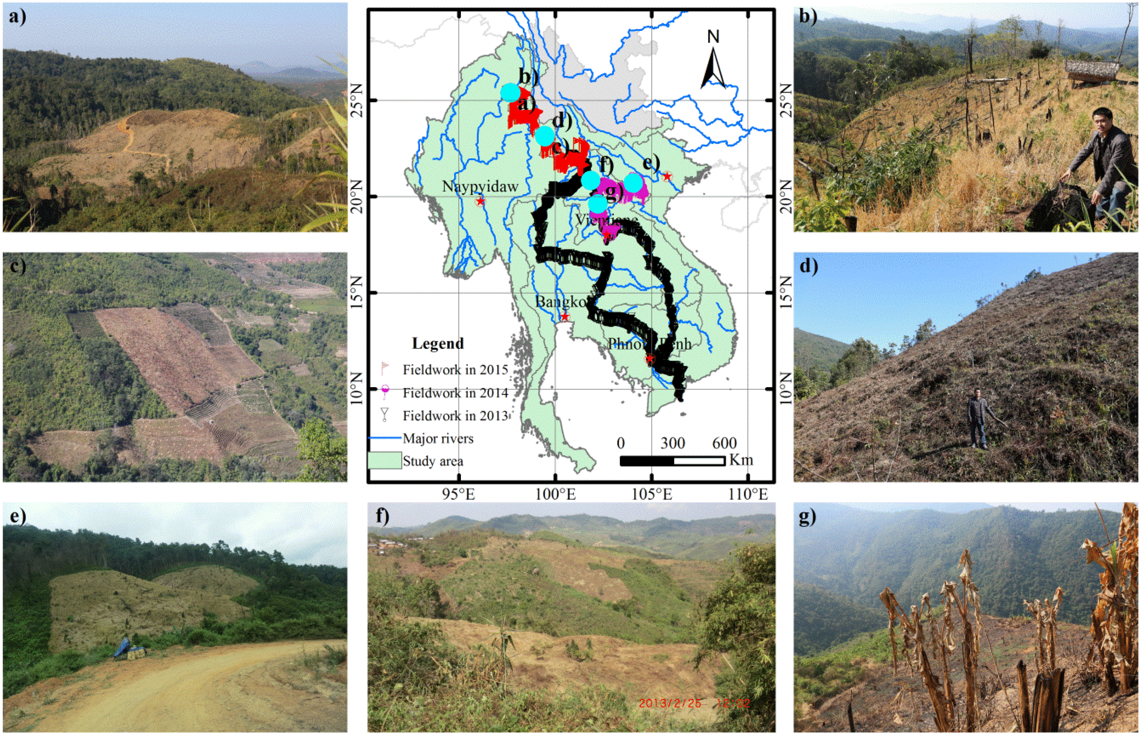
2.1. Study Area
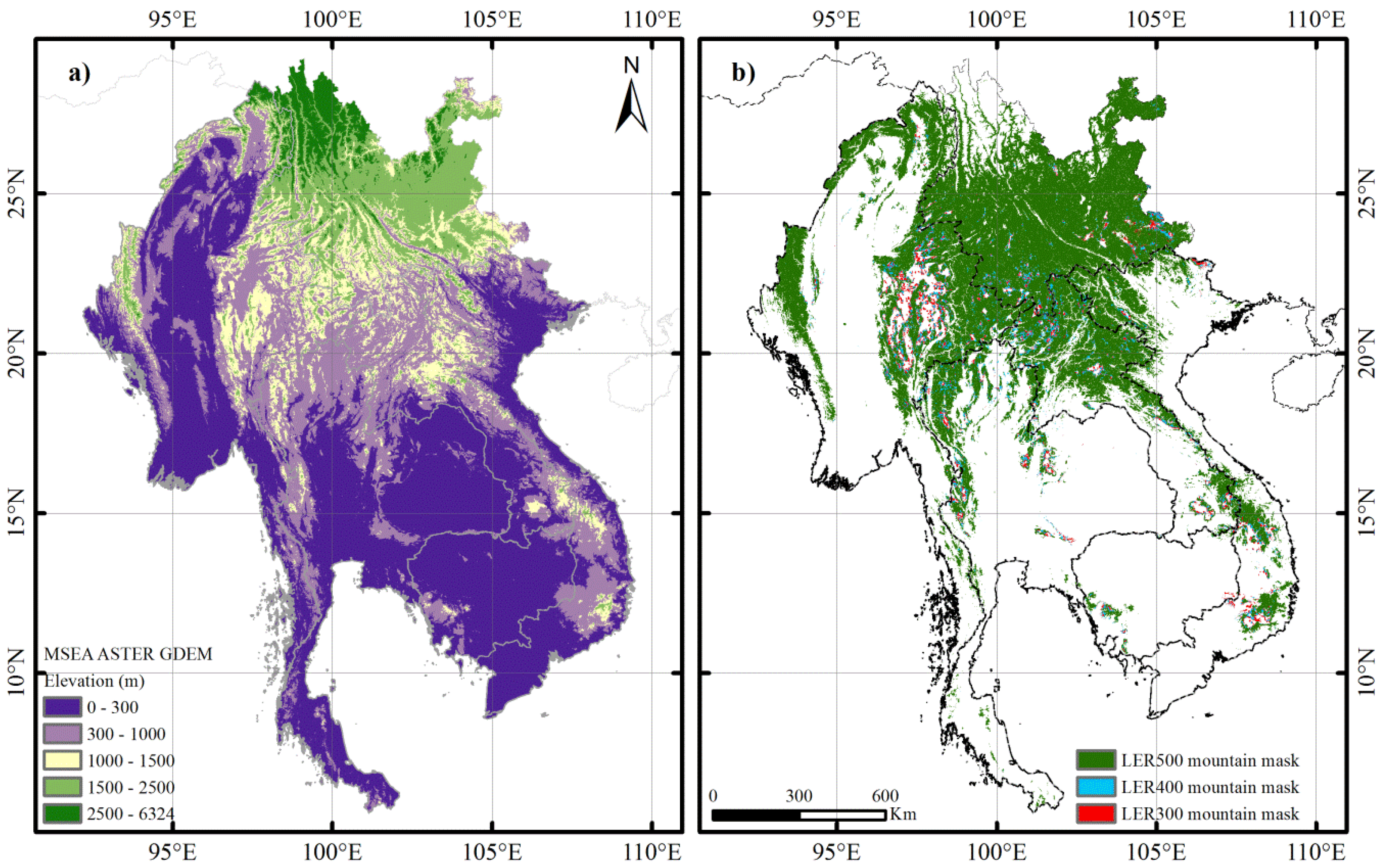
2.2. Topographical Data Products and Mountain Area Definition in MSEA
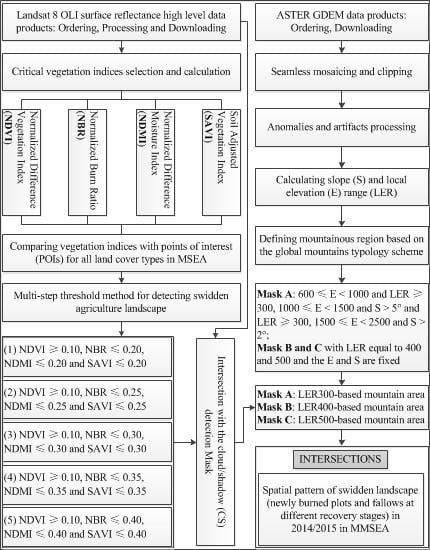
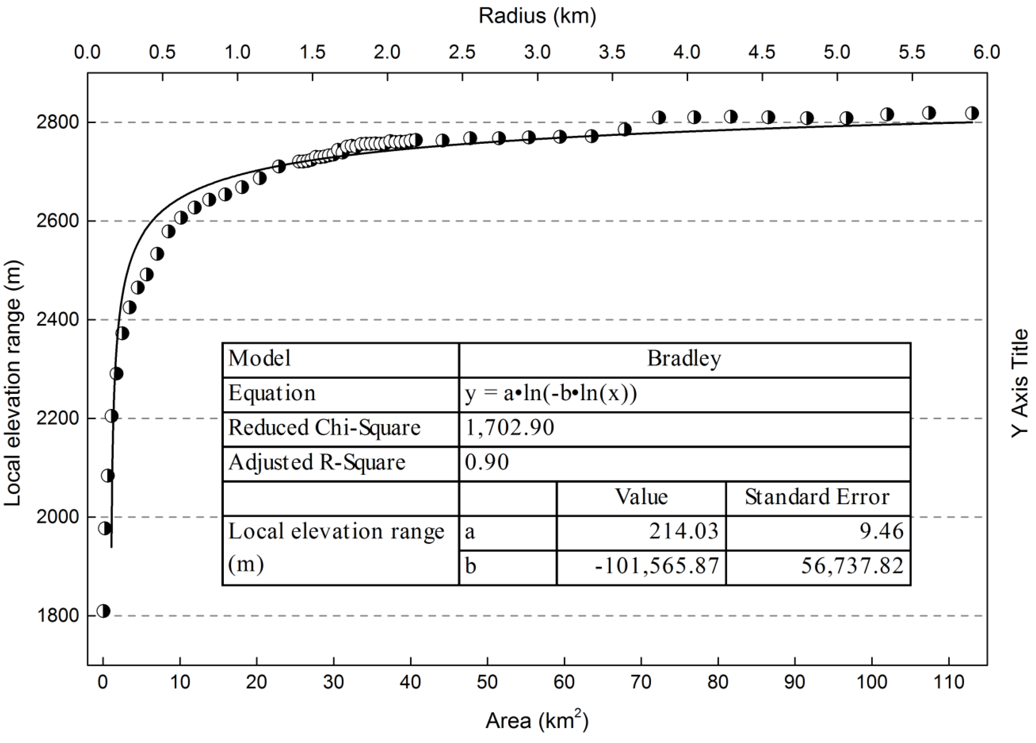
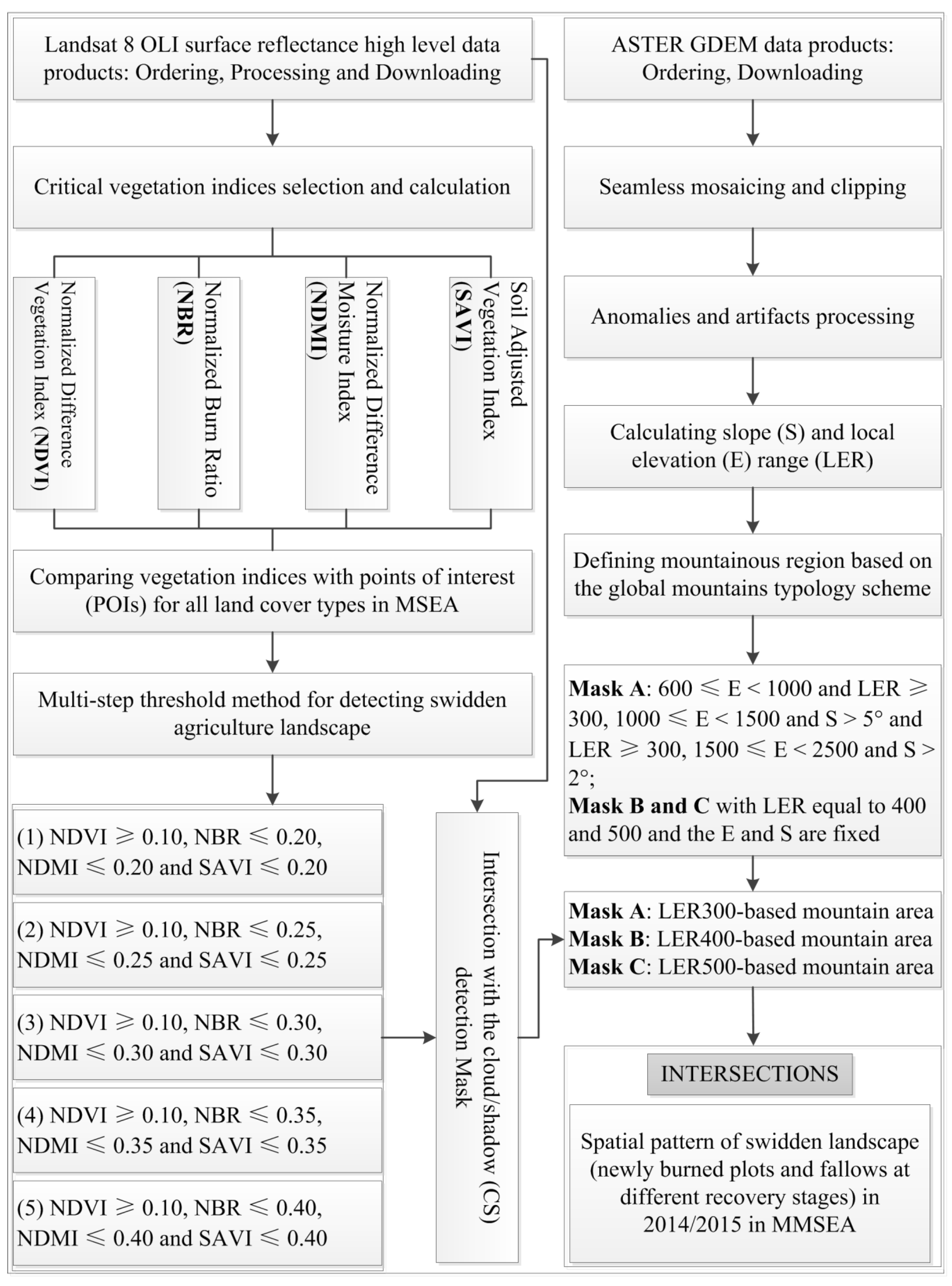
2.2.1. Data Acquisition and Anomaly Values Processing

2.2.2. Defining the Mountainous Area in MSEA

| Mountain Classes | Typology (UNEP-WCMC) | Typology in This Study | ||||
|---|---|---|---|---|---|---|
| Elevation (m) | Slope and LER | Elevation (m) | Slope and LER | Area | ||
| (104 km2) | (%) | |||||
| 1 | ≥2500 | - | ≥2500 | - | 6.62 | 2.84 |
| 2 | 1500–2499 | Slope ˃ 2° | 1500–2499 | Slope ˃ 2° | 23.30 | 9.99 |
| 3 | 1000–1499 | Slope ˃ 5° and LER ≥ 300 m | 1000–1499 | Slope ˃ 5° and LER ≥ 300 m | 23.22 | 9.96 |
| Slope ˃ 5° and LER ≥ 400 m | 22.29 | 9.56 | ||||
| Slope ˃ 5° and LER ≥ 500 m | 20.76 | 8.90 | ||||
| 4 | 300–1000 | LER ≥ 300 m | 600–1000 | LER ≥ 300 m LER ≥ 400 m LER ≥ 500 m | 52.59 | 22.55 |
| 46.93 | 20.12 | |||||
| 39.66 | 17.00 | |||||

2.3. Landsat-8 OLI Imagery and Pre-Processing
2.4. Fieldwork on the Collection of Ground Truth Data in MSEA
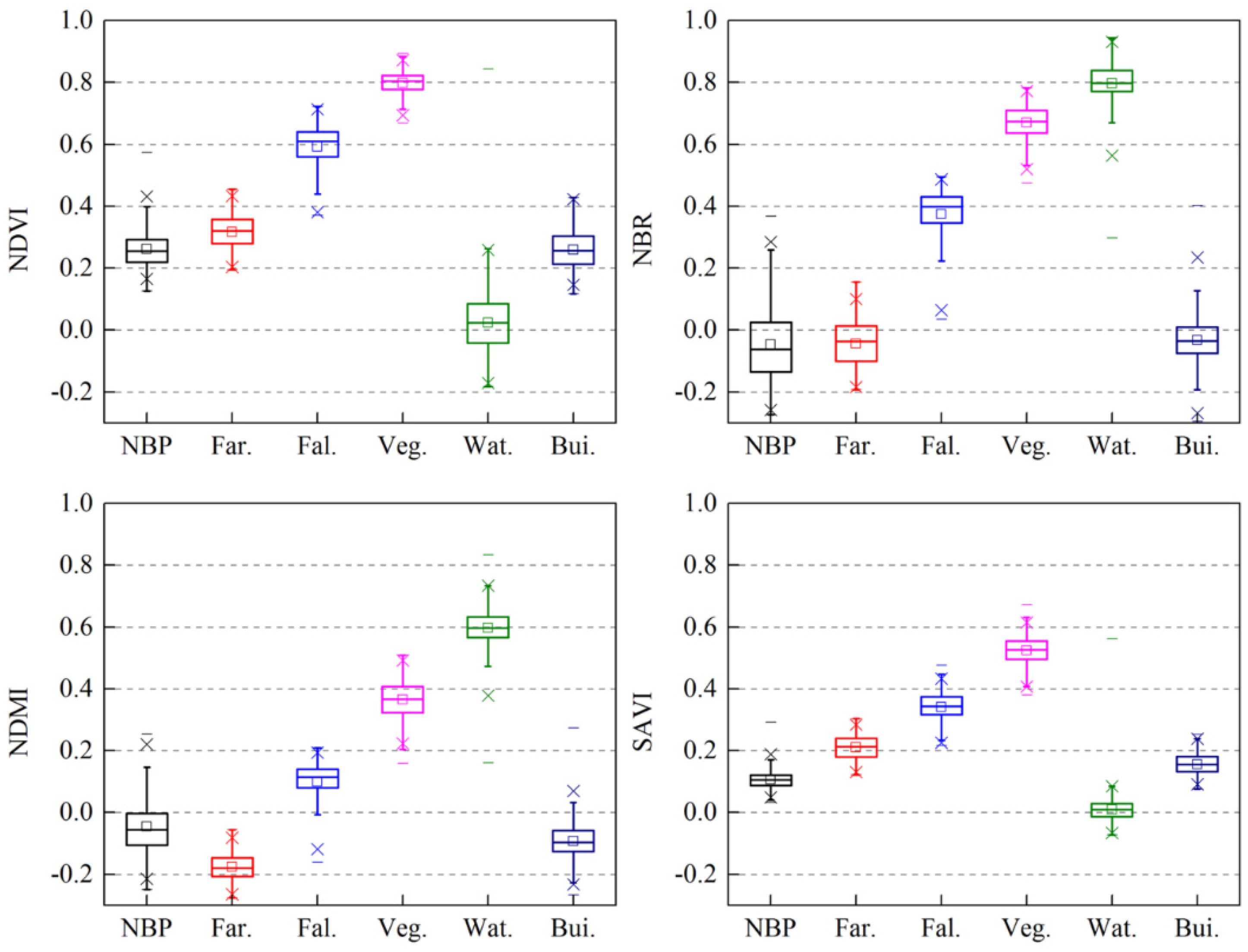
2.5. Training Sampling and Swidden Landscape-Detecting Algorithms


| VI Step | NDVI | NBR | NDMI | SAVI | Stage |
|---|---|---|---|---|---|
| 1 | ≥0.10 | ≤0.20 | ≤0.20 | ≤0.20 | Newly-opened swidden |
| 2 | ≥0.10 | ≤0.25 | ≤0.25 | ≤0.25 | Swidden fallow (Stage 1) |
| 3 | ≥0.10 | ≤0.30 | ≤0.30 | ≤0.30 | Swidden fallow (Stage 2) |
| 4 | ≥0.10 | ≤0.35 | ≤0.35 | ≤0.35 | Swidden fallow (Stage 3) |
| 5 | ≥0.10 | ≤0.40 | ≤0.40 | ≤0.40 | Swidden fallow (Stage 4) |
2.6. Validation
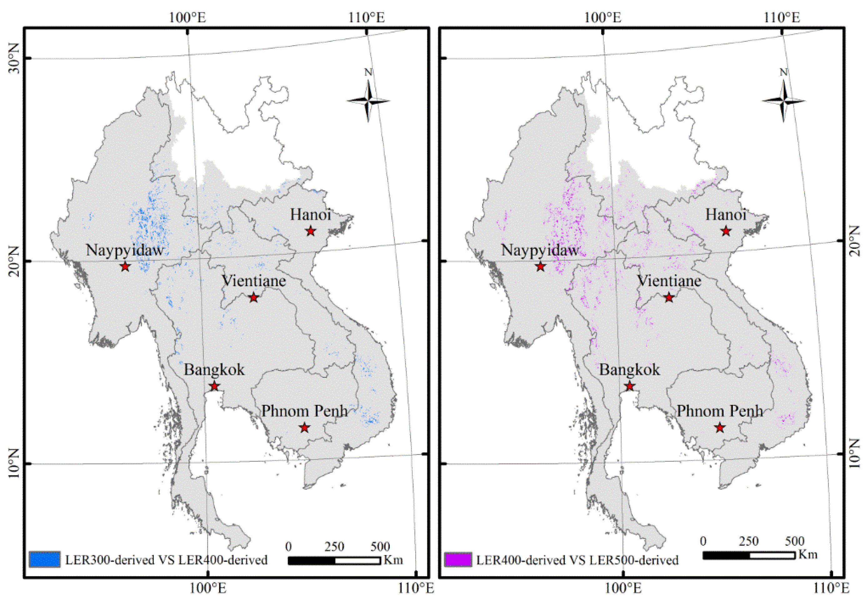
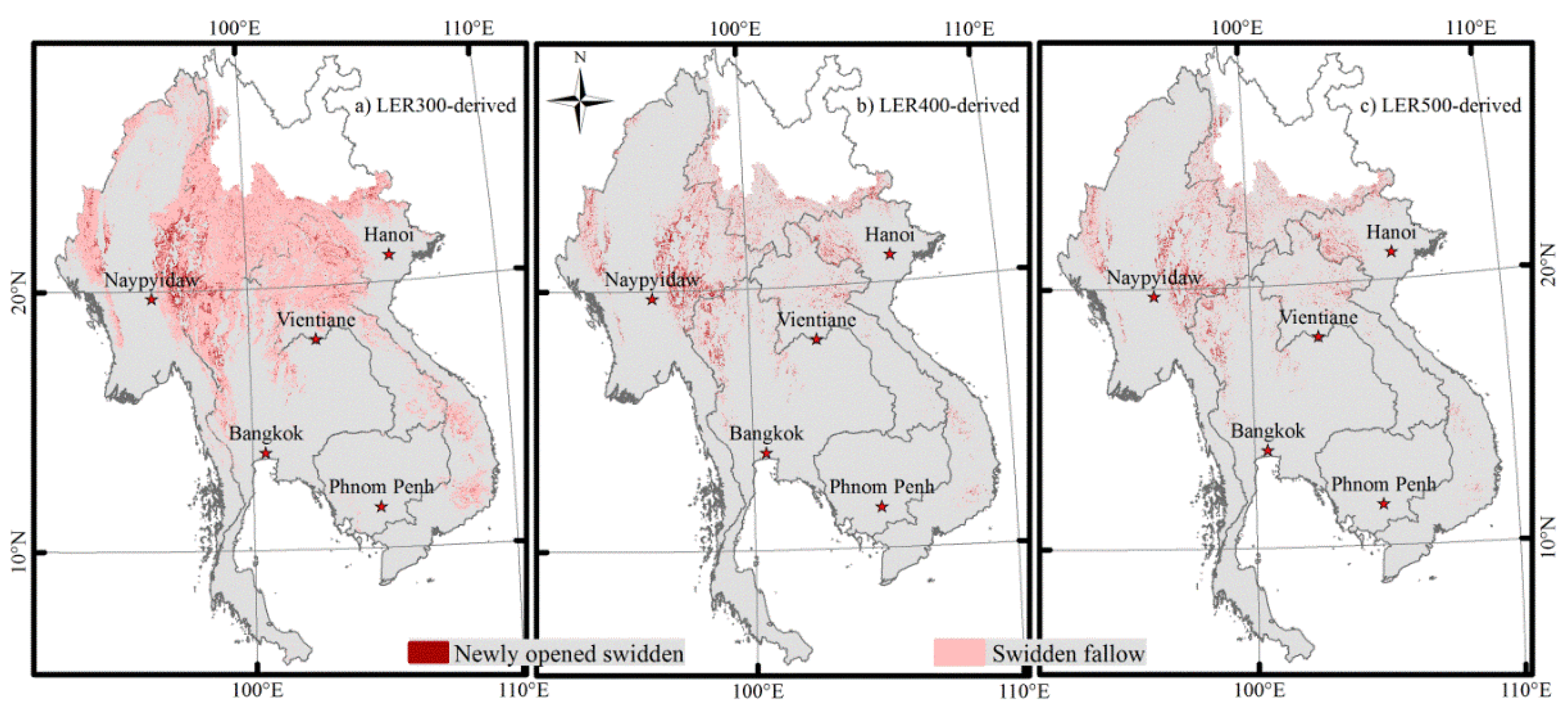
3. Results
| Area (km2) | Proportion (%) of the Total Land Area in MSEA | Range | ||||||
|---|---|---|---|---|---|---|---|---|
| LER300 | LER400 | LER500 | LER300 | LER400 | LER500 | |||
| Newly opened swidden | 32,803 | 28,234 | 23,688 | 1.41 | 1.21 | 1.02 | 0.16 | 0.16 |
| Swidden fallow (Stage 1) | 64,279 | 56,342 | 47,934 | 2.76 | 2.42 | 2.05 | 0.14 | 0.15 |
| Swidden fallow (Stage 2) | 100,731 | 89,866 | 77,686 | 4.32 | 3.85 | 3.33 | 0.12 | 0.14 |
| Swidden fallow (Stage 3) | 135,370 | 122,396 | 107,149 | 5.80 | 5.25 | 4.59 | 0.11 | 0.12 |
| Swidden fallow (Stage 4) | 167,282 | 152,788 | 135,027 | 7.17 | 6.55 | 5.79 | 0.09 | 0.12 |

| Class | Total No. of Ground Reference Pixels | Total No. of Classified Pixels | Producer’s Accuracy (%) | ||
|---|---|---|---|---|---|
| Swidden Fields | Permanent Farmland | ||||
| Classified Results | Swidden fields | 126,624 | 24,348 | 150,972 | 83.9 |
| Permanent farmland | 2380 | 50,259 | 52,639 | 95.5 | |
| Total No. of Ground Reference Pixels | 129,004 | 74,607 | 203,611 | ||
| User’s Accuracy (%) | 98.2 | 67.4 | |||
4. Discussion
5. Couclusions
Acknowledgments
Author Contributions
Conflicts of Interest
References
- Mertz, O.; Padoch, C.; Fox, J.; Cramb, R.; Leisz, S.; Lam, N.; Vien, T. Swidden change in Southeast Asia: Understanding causes and consequences. Hum. Ecol. 2009, 37, 259–264. [Google Scholar] [CrossRef]
- Li, P.; Feng, Z.; Jiang, L.; Liao, C.; Zhang, J. A review of swidden agriculture in Southeast Asia. Remote Sens. 2014, 6, 1654–1683. [Google Scholar] [CrossRef]
- Cairns, M.F. Shifting Cultivation and Environmental Change: Indigenous People, Agriculture and Forest Conservation; Routledge: New York, NY, USA, 2015. [Google Scholar]
- Vadrevu, K.P.; Justice, C.O. Vegetation fires in the Asian region: Satellite observational needs and priorities. Glob. Environ. Res. 2011, 15, 65–76. [Google Scholar]
- van Vliet, N.; Mertz, O.; Birch-Thomsen, T.; Schmook, B. Is there a continuing rationale for swidden cultivation in the 21st Century? Hum. Ecol. 2013, 41, 1–5. [Google Scholar] [CrossRef]
- Schmidt-Vogt, D.; Leisz, S.J.; Mertz, O.; Heinimann, A.; Thiha, T.; Messerli, P.; Epprecht, M.; Cu, P.V.; Chi, V.K.; Hardiono, M.; Dao, T.M. An assessment of trends in the extent of swidden in Southeast Asia. Hum. Ecol. 2009, 37, 269–280. [Google Scholar] [CrossRef]
- Padoch, C.; Coffey, K.; Mertz, O.; Leisz, S.J.; Fox, J.; Wadley, R.L. The demise of swidden in Southeast Asia? Local realities and regional ambiguities. Geogr. Tidsskr.-Dan. J. Geogr. 2007, 107, 29–41. [Google Scholar] [CrossRef]
- Cramb, R.; Colfer, C.; Dressler, W.; Laungaramsri, P.; Le, Q.; Mulyoutami, E.; Peluso, N.; Wadley, R. Swidden transformations and rural livelihoods in Southeast Asia. Hum. Ecol. 2009, 37, 323–346. [Google Scholar] [CrossRef]
- Van Vliet, N.; Mertz, O.; Heinimann, A.; Langanke, T.; Pascual, U.; Schmook, B.; Adams, C.; Schmidt-Vogt, D.; Messerli, P.; Leisz, S.; et al. Trends, drivers and impacts of changes in swidden cultivation in tropical forest-agriculture frontiers: A global assessment. Glob. Environ. Chang. 2012, 22, 418–429. [Google Scholar] [CrossRef]
- FAO Staff. Shifting cultivation. Unasylva 1957, 11, 9–11. [Google Scholar]
- Sprenger, G. Out of the ashes: Swidden cultivation in highland Laos. Anthropol. Today 2006, 22, 9–13. [Google Scholar] [CrossRef]
- Fox, J.; Fujita, Y.; Ngidang, D.; Peluso, N.; Potter, L.; Sakuntaladewi, N.; Sturgeon, J.; Thomas, D. Policies, political-economy, and swidden in Southeast Asia. Hum. Ecol. 2009, 37, 305–322. [Google Scholar] [CrossRef]
- Rerkasem, K.; Lawrence, D.; Padoch, C.; Schmidt-Vogt, D.; Ziegler, A.D.; Bruun, T.B. Consequences of swidden transitions for crop and fallow biodiversity in Southeast Asia. Hum. Ecol. 2009, 37, 347–360. [Google Scholar] [CrossRef]
- Bruun, T.B.; de Neergaard, A.; Lawrence, D.; Ziegler, A.D. Environmental consequences of the demise in swidden cultivation in Southeast Asia: Carbon storage and soil quality. Hum. Ecol. 2009, 37, 375–388. [Google Scholar] [CrossRef]
- Ziegler, A.D.; Bruun, T.B.; Guardiola-Claramonte, M.; Giambelluca, T.W.; Lawrence, D.; Lam, N.T. Environmental consequences of the demise in swidden cultivation in Montane Mainland Southeast Asia: Hydrology and geomorphology. Hum. Ecol. 2009, 37, 361–373. [Google Scholar] [CrossRef]
- Padoch, C.; Pinedo-Vasquez, M. Saving slash-and-burn to save biodiversity. Biotropica 2010, 42, 550–552. [Google Scholar] [CrossRef]
- Justice, C.O.; Giglio, L.; Korontzi, S.; Owens, J.; Morisette, J.T.; Roy, D.; Descloitres, J.; Alleaume, S.; Petitcolin, F.; Kaufman, Y. The MODIS fire products. Remote Sens. Environ. 2002, 83, 244–262. [Google Scholar] [CrossRef]
- Langner, A.; Miettinen, J.; Siegert, F. Land cover change 2002–2005 in Borneo and the role of fire derived from MODIS imagery. Glob. Chang. Biol. 2007, 13, 2329–2340. [Google Scholar] [CrossRef]
- Müller, D.; Suess, S.; Hoffmann, A.A.; Buchholz, G. The value of satellite-based active fire data for monitoring, reporting and verification of REDD+ in the Lao PDR. Hum. Ecol. 2013, 41, 7–20. [Google Scholar] [CrossRef]
- Hurni, K.; Hett, C.; Heinimann, A.; Messerli, P.; Wiesmann, U. Dynamics of shifting cultivation landscapes in Northern Lao PDR Between 2000 and 2009 based on an analysis of MODIS time series and landsat images. Hum. Ecol. 2013, 41, 21–36. [Google Scholar] [CrossRef]
- Bastarrika, A.; Chuvieco, E.; Martín, M.P. Mapping burned areas from Landsat TM/ETM+ data with a two-phase algorithm: Balancing omission and commission errors. Remote Sens. Environ. 2011, 115, 1003–1012. [Google Scholar] [CrossRef]
- Fuller, D.O. Tropical forest monitoring and remote sensing: A new era of transparency in forest governance? Singap. J. Trop. Geogr. 2006, 27, 15–29. [Google Scholar] [CrossRef]
- Roy, D.P.; Wulder, M.A.; Loveland, T.R.; Woodcock, C.E.; Allen, R.G.; Anderson, M.C.; Helder, D.; Irons, J.R.; Johnson, D.M.; Kennedy, R. Landsat-8: Science and product vision for terrestrial global change research. Remote Sens. Environ. 2014, 145, 154–172. [Google Scholar] [CrossRef]
- Conant, F.P.; Cary, T.K. A first interpretation of East African swiddening via computer. In Presented at Symposium on Machine Processing of Remotely Sensed Data, Purdue, IN, USA, 21–23 June 1977; 1977; pp. 36–42. [Google Scholar]
- Li, P.; Jiang, L.; Feng, Z. Cross-comparison of vegetation indices derived from Landsat-7 Enhanced Thematic Mapper Plus (ETM+) and Landsat-8 Operational Land Imager (OLI) Sensors. Remote Sens. 2014, 6, 310–329. [Google Scholar] [CrossRef]
- Li, P.; Feng, Z. Monitoring phenological stages of swiddening in northern Laos during the dry season. Proc. SPIE 2014. [Google Scholar] [CrossRef]
- Woodcock, C.E.; Allen, R.; Anderson, M.; Belward, A.; Bindschadler, R.; Cohen, W.; Gao, F.; Goward, S.N.; Helder, D.; Helmer, E.; et al. Free access to Landsat imagery. Science 2008, 320, 1011–1012. [Google Scholar] [CrossRef] [PubMed]
- Leisz, S.J.; Rasmussen, M.S. Mapping fallow lands in Vietnam’s north-central mountains using yearly Landsat imagery and a land-cover succession model. Int. J. Remote Sens. 2012, 33, 6281–6303. [Google Scholar] [CrossRef]
- Robichaud, W.G.; Sinclair, A.R.; Odarkor-Lanquaye, N.; Klinkenberg, B. Stable forest cover under increasing populations of swidden cultivators in central Laos: The roles of intrinsic culture and extrinsic wildlife trade. Ecol. Soc. 2009, 14, 33–34. [Google Scholar]
- Tucker, C.J. Red and photographic infrared linear combinations for monitoring vegetation. Remote Sens. Environ. 1979, 8, 127–150. [Google Scholar] [CrossRef]
- Pereira, J.M. A comparative evaluation of NOAA/AVHRR vegetation indexes for burned surface detection and mapping. IEEE Trans. Geosci. Remote Sens. 1999, 37, 217–226. [Google Scholar] [CrossRef]
- Chuvieco, E.; Martin, M.P.; Palacios, A. Assessment of different spectral indices in the red-near-infrared spectral domain for burned land discrimination. Int. J. Remote Sens. 2002, 23, 5103–5110. [Google Scholar] [CrossRef]
- Hardisky, M.A.; Klemas, V.; Smart, R.M. The influence of soil salinity, growth form and leaf moisture on the spectral radiance of Spartina alterniflora canopies. Photogramm. Eng. Remote Sens. 1983, 49, 77–83. [Google Scholar]
- Xiao, X.; Chandrashekhar, B.; Audrey, W.; Sage, S.; Chen, Y. Recovery of vegetation canopy after severe fire in 2000 at the Black Hills National Forest, South Dakota, USA. J. Res. Ecol. 2011, 2, 106–116. [Google Scholar]
- García, M.L.; Caselles, V. Mapping burns and natural reforestation using Thematic Mapper data. Geoc. Int. 1991, 6, 31–37. [Google Scholar] [CrossRef]
- Huete, A.R. A soil-adjusted vegetation index (SAVI). Remote Sens. Environ. 1988, 25, 295–309. [Google Scholar] [CrossRef]
- Fox, J.; Castella, J.; Ziegler, A.D. Swidden, rubber and carbon: Can REDD plus work for people and the environment in Montane Mainland Southeast Asia? Glob. Environ.Chang.-Hum. Policy Dimens. 2014, 29, 318–326. [Google Scholar] [CrossRef]
- Stibig, H.J.; Achard, F.; Fritz, S. A new forest cover map of continental southeast Asia derived from SPOT-VEGETATION satellite imagery. Appl. Veg. Sci. 2004, 7, 153–162. [Google Scholar] [CrossRef]
- Stibig, H.J.; Belward, A.S.; Roy, P.S.; Rosalina, W.U.; Agrawal, S.; Joshi, P.K.; Beuchle, R.; Fritz, S.; Mubareka, S.; Giri, C. A land-cover map for South and Southeast Asia derived from SPOT-VEGETATION data. J. Biogeogr. 2007, 34, 625–637. [Google Scholar] [CrossRef]
- Rerkasem, K.; Yimyam, N.; Rerkasem, B. Land use transformation in the mountainous mainland Southeast Asia region and the role of indigenous knowledge and skills in forest management. For. Ecol. Manag. 2009, 257, 2035–2043. [Google Scholar] [CrossRef]
- Fox, J.; Vogler, J.B. Land-use and land-cover change in montane mainland southeast Asia. Environ. Manag. 2005, 36, 394–403. [Google Scholar] [CrossRef] [PubMed]
- Weinstock, J.A. The Future of Swidden Cultivation. In Shifting Cultivation and Environmental Change: Indigenous People, Agriculture and Forest Conservation; Cairns, M., Ed.; Routledge: New York, NY, USA, 2015; pp. 179–185. [Google Scholar]
- Tachikawa, T.; Hato, M.; Kaku, M.; Iwasaki, A. Characteristics of ASTER GDEM version 2. In Proceedings of the 2011 IEEE International Geoscience and Remote Sensing Symposium, Vancouver, BC, Canada, 24–29 July 2011; pp. 3657–3660.
- Shi, Y.; Yamaguchi, Y. A high-resolution and multi-year emissions inventory for biomass burning in Southeast Asia during 2001–2010. Atmos. Environ. 2014, 98, 8–16. [Google Scholar] [CrossRef]
- Kapos, V.; Rhind, J.; Edwards, M.; Price, M.F.; Ravilious, C.; Butt, N. Developing a map of the world's mountain forests. In Forests in Sustainable Mountain Development: A State of Knowledge Report for 2000. Task Force on Forests in Sustainable Mountain Development; Martin, F.P., Nathalie, B., Eds.; Oxford University: Oxford, UK, 2000; pp. 4–19. [Google Scholar]
- Platts, P.J.; Burgess, N.D.; Gereau, R.E.; Lovett, J.C.; Marshall, A.R.; McClean, C.J.; Pellikka, P.K.; Swetnam, R.D.; Marchant, R. Delimiting tropical mountain ecoregions for conservation. Environ. Conserv. 2011, 38, 312–324. [Google Scholar] [CrossRef]
- Fjeldså, J.; Bowie, R.C.; Rahbek, C. The role of mountain ranges in the diversification of birds. Ann. Rev. Ecol. Evol. Syst. 2012, 43, 249–265. [Google Scholar] [CrossRef]
- USGS Global Visualization Viewer. Available online: http://glovis.usgs.gov (accessed on 10 June 2015).
- The Land Satellite Data Systems (LSDS) Science Research and Development (LSRD). Available online: https://espa.cr.usgs.gov/ (accessed on 10 July 2015).
- Zhu, Z.; Wang, S.; Woodcock, C.E. Improvement and expansion of the Fmask algorithm: Cloud, cloud shadow, and snow detection for Landsats 4–7, 8, and Sentinel 2 images. Remote Sens. Environ. 2015, 159, 269–277. [Google Scholar] [CrossRef]
- Dong, J.; Xiao, X.; Kou, W.; Qin, Y.; Zhang, G.; Li, L.; Jin, C.; Zhou, Y.; Wang, J.; Biradar, C. Tracking the dynamics of paddy rice planting area in 1986–2010 through time series Landsat images and phenology-based algorithms. Remote Sens. Environ. 2015, 160, 99–113. [Google Scholar] [CrossRef]
- Liu, X.; Feng, Z.; Jiang, L.; Li, P.; Liao, C.; Yang, Y.; You, Z. Rubber plantation and its relationship with topographical factors in the border region of China, Laos and Myanmar. J. Geogr. Sci. 2013, 23, 1019–1040. [Google Scholar] [CrossRef]
- Li, P.; Zhang, J.; Feng, Z. Mapping rubber tree plantations using a Landsat-based phenological algorithm in Xishuangbanna, southwest China. Remote Sens. Lett. 2015, 6, 49–58. [Google Scholar] [CrossRef]
- Yin, L.; Xue, D.; Wang, J. Rubber plantation, swidden agriculture and indigenous knowledge: A case study of a bulang village in Xishuangbanna, China. In Shifting Cultivation and Environmental Change: Indigenous People, Agriculture and Forest Conservation; Cairns, M., Ed.; Routledge: New York, NY, USA, 2015; pp. 811–825. [Google Scholar]
- Liao, C.; Feng, Z.; Li, P.; Zhang, J. Monitoring the spatio-temporal dynamics of swidden agriculture and fallow vegetation recovery using Landsat imagery in northern Laos. J. Geogr. Sci. 2015, 25, 1218–1234. [Google Scholar] [CrossRef]
- Trakansuphakon, P. Changing strategies of shifting cultivators to match a changing climate. In Shifting Cultivation and Environmental Change: Indigenous People, Agriculture and Forest Conservation; Cairns, M., Ed.; Routledge: New York, NY, USA, 2015; pp. 335–356. [Google Scholar]
- Hurni, K.; Hett, C.; Epprecht, M.; Messerli, P.; Heinimann, A. A texture-based land cover classification for the delineation of a shifting cultivation landscape in the Lao PDR using landscape metrics. Remote Sens. 2013, 5, 3377–3396. [Google Scholar] [CrossRef]
© 2016 by the authors; licensee MDPI, Basel, Switzerland. This article is an open access article distributed under the terms and conditions of the Creative Commons by Attribution (CC-BY) license (http://creativecommons.org/licenses/by/4.0/).
Share and Cite
Li, P.; Feng, Z. Extent and Area of Swidden in Montane Mainland Southeast Asia: Estimation by Multi-Step Thresholds with Landsat-8 OLI Data. Remote Sens. 2016, 8, 44. https://doi.org/10.3390/rs8010044
Li P, Feng Z. Extent and Area of Swidden in Montane Mainland Southeast Asia: Estimation by Multi-Step Thresholds with Landsat-8 OLI Data. Remote Sensing. 2016; 8(1):44. https://doi.org/10.3390/rs8010044
Chicago/Turabian StyleLi, Peng, and Zhiming Feng. 2016. "Extent and Area of Swidden in Montane Mainland Southeast Asia: Estimation by Multi-Step Thresholds with Landsat-8 OLI Data" Remote Sensing 8, no. 1: 44. https://doi.org/10.3390/rs8010044