Article

Synergistic Use of LiDAR and APEX Hyperspectral Data for High-Resolution Urban Land Cover Mapping

Cartography and GIS Research Group, Vrije Universiteit Brussel, Brussel 1050, Belgium
*
Author to whom correspondence should be addressed.
Remote Sens. 2016, 8(10), 787; https://doi.org/10.3390/rs8100787
Submission received: 7 June 2016 / Revised: 22 August 2016 / Accepted: 8 September 2016 / Published: 22 September 2016

Abstract

:
Land cover mapping of the urban environment by means of remote sensing remains a distinct challenge due to the strong spectral heterogeneity and geometric complexity of urban scenes. Airborne imaging spectroscopy and laser altimetry have each made remarkable contributions to urban mapping but synergistic use of these relatively recent data sources in an urban context is still largely underexplored. In this study a synergistic workflow is presented to cope with the strong diversity of materials in urban areas, as well as with the presence of shadow. A high-resolution APEX hyperspectral image and a discrete waveform LiDAR dataset covering the Eastern part of Brussels were made available for this research. Firstly, a novel shadow detection method based on LiDAR intensity-APEX brightness thresholding is proposed and compared to commonly used approaches for shadow detection. A combination of intensity-brightness thresholding with DSM model-based shadow detection is shown to be an efficient approach for shadow mask delineation. To deal with spectral similarity of different types of urban materials and spectral distortion induced by shadow cover, supervised classification of shaded and sunlit areas is combined with iterative LiDAR post-classification correction. Results indicate that height, slope and roughness features contribute to improved classification accuracies in descending order of importance. Results of this study illustrate the potential of synergistic application of hyperspectral imagery and LiDAR for urban land cover mapping.

Graphical Abstract

1. Introduction

In light of the challenges presented by climate change and urbanization, more than ever urban areas need to be monitored in order to gain a better physical understanding of this complex and dynamic environment. Over the past decades, urban remote sensing has presented itself as a viable means to systematically acquire information on different spatial, spectral and temporal scales using a wide range of spaceborne and airborne Earth observation platforms. Remote sensing of urban scenes remains a challenging topic though due to characteristic difficulties presented by the urban environment and limitations of traditional sensors. Urban areas are composed of a complex mosaic of different materials that can usually be attributed to a combination of four material components: minerals, vegetation, oil-derived products and other artificial materials including metals [1]. Each material displays specific reflectance features in the Visible Near-Infrared (VNIR) and Short Wave Infrared (SWIR) wavelength regions so consequently cities are characterized by a very high degree of spectral heterogeneity [2,3]. Adding to the complexity is the fact that some materials that are used for different purposes (e.g., roof versus road materials) do share similar material compositions and thus also show similar spectral behavior [4]. Variations in composition within a material type, material weathering and material condition can furthermore induce a significant degree of spectral intra-class confusion [5,6,7,8]. Another concern of urban remote sensing is the complex geometry of the urban environment. Most observed urban objects tend to have rather small spatial dimensions compared to objects encountered in natural environments and these objects are often arranged in complex site-specific geometries [1,4]. The characteristic geometric assembly and the differences in surface roughness of urban areas result in substantial impact of direction-dependent reflectance properties and in the presence of shade. Both these phenomena lead to a substantial increase in heterogeneity in the measured spectral response of urban materials [8].
The complexity of urban scenes has led to an increased demand for more advanced, high resolution remote sensing solutions. Especially in the past decade there has been a steady growth in the development and availability of new sensors able to better cope with the challenges outlined above. Two technologies that have made remarkable contributions are hyperspectral remote sensing, also referred to as imaging spectroscopy, and Light Detection And Ranging (LiDAR) [9,10,11]. As opposed to broadband multispectral sensors, hyperspectral sensors tend to extensively cover both the VNIR and SWIR regions with a high number (ranging from tens to hundreds) of narrowly defined spectral bands, allowing them to capture even subtle spectral features, strongly improving the ability to discriminate different materials and in some cases even material conditions [10]. LiDAR technology can be described as a laser profiling and scanning system emitting monochromatic NIR pulses that produce very dense point clouds in which each point is accurately positioned in 3D using direct geo-referencing. As such, LiDAR is a powerful tool for altimetric modelling of nearly any terrain [9]. The advent of LiDAR marked a major step forward in urban remote sensing since it allowed to move beyond the limits dictated by multi- and hyperspectral imagery by adding new components to the equation such as height, intensity and multiple return/texture features [9,12,13,14,15].
Despite the merits that hyperspectral and LiDAR data possess on their own, it is mainly through synergistic use of both these technologies that urban mapping has managed to produce some of its most interesting and promising results in recent years [16,17,18,19,20]. Data fusion of imaging spectroscopy and laser altimetry or hyperspectral-LiDAR synergy is a young but dynamic research field that has only started to develop fully in the last decade. Approaches for synergy can be differentiated based on how the LiDAR data are integrated in the land-cover mapping workflow: through vector stacking (feature selection or pre-processing), re-classification or in a post-classification phase [21]. Vector stacking should be understood as a process of combining raw spectral, textural or object-based features derived from a hyperspectral image and a LiDAR point cloud before being used as input for a classifier [22]. Given the completely different nature of hyperspectral and LiDAR data, machine learning classifiers are preferred in this approach, since these classifiers are non-parametric and do not make assumptions regarding the distribution of the input variables [23]. Re-classification involves a two-step mapping process where the first step consists of a classification based on hyperspectral data, which is followed by a second classification using the output of the spectral classifier and LiDAR derived features as its input. More than just improving the accuracy of the spectral classification, adding height (derived) information can improve thematic detail in land cover mapping [18]. Finally, post-classification involves the improvement of classification output using external data (in this case LiDAR) in combination with a specific ruleset. Rulesets for post-classification can be constructed manually or semi-automatically using discrete thresholds, soft classification output, object-based and/or statistical information in order to perform correction [24]. A number of examples can be found in the literature where multiple approaches for hyperspectral-LiDAR synergy are combined within one workflow [17,18]. Regardless of the approach, LiDAR height information and derivatives naturally complement hyperspectral data because they may allow discriminating between geometrically dissimilar but spectrally similar material classes.
Use of LiDAR data in combination with hyperspectral data may also prove useful for dealing with the omnipresence of shadow in urban areas. Shadow is the result of a complete or partial blocking of direct irradiance. It is particularly problematic for analysis of imagery covering cities with a strong degree of high-rise development or strong topographic features. Likewise, imagery acquired before or after solar noon, outside of the summer season, during cloudy weather conditions or in temperate to arctic climate zones may be severely tainted by shadow [25,26]. Whereas for sunlit surfaces direct irradiance will be the main contributing factor to the total radiance budget, for shaded areas the relative contributions of environmental and atmospheric radiance will be far greater while direct irradiance may even be reduced to zero [27]. Because shadow distorts the spectral signature of materials, accurate mapping of urban areas requires dedicated approaches to deal with shadow. A distinction can be made between shadow detection and shadow compensation techniques. Shadow detection answers the question where and to what extent shadow occurs in an image [28]. Shadow compensation on the other hand encompasses methods that can be used to reduce or avoid the impact of shadow cover on mapping [29]. A considerable number of shadow detection and compensation techniques have been developed for remote sensing but most focus on high resolution multispectral data. Only more recently have techniques been proposed that attempt to benefit from LiDAR and hyperspectral imagery. Model-based or geometric shadow detection approaches utilize a-priori information, in most cases Digital Surface Models (DSM) and solar illumination angles at the time of image acquisition, to perform line-of-sight analysis or ray tracing [30,31,32,33]. These geometric approaches have the advantage of avoiding errors in shadow detection induced by spectral confusion but their output will be directly dependent on the quality of the DSM and its co-registration with the image data. Color Invariant approaches, on the other hand, select certain image bands, spectral indices or color space components that are (near) insensitive to lighting conditions and compare those with light dependent features [34]. Machine learning shadow detection relies on the unique spectral characteristics of shaded materials to detect shadow induced spectral features. Support Vector Machines (SVM) are currently prevalent classification algorithms used for this purpose [35]. The main drawback of the machine learning approach, however, is the need to produce a dedicated training dataset of shaded areas, which can be very difficult and labor intensive. Machine learning shadow detection methods will be inclined to produce more satisfying results when used with high resolution spectral information, but will in any case still be prone to spectral confusion [28,29].
Shadow compensation includes a wide range of methods. A differentiation can be made between pre-processing, classification and post-processing techniques. Illumination effects in hyperspectral imagery can be suppressed in pre-processing by converting radiance or reflectance information to spectral angles and linearly correcting them based on shadow/non-shadow statistics [36]. A more intricate method to compensate for the effect of shadow in hyperspectral urban imagery using LiDAR information has been proposed in [37]. Here, a DSM and other LiDAR derived features such as sky view factor are used to model different irradiance components which are in turn entered in a non-linear spectral correction model. Direct classification or classification of shaded areas using shaded material training data is a shadow compensation technique that has been applied with relative success for classifying multispectral imagery [38] but remains remarkably unexplored for hyperspectral data. This approach relies on the idea that radiances received from shaded areas are still material dependent and assumes that a significant amount of class related spectral information is still present in shadow [28]. Shadow compensation can also be achieved in a post-classification phase by training a machine learning classifier with a separate shadow class and then running a second, dedicated classifier to assign shadow pixels identified in the first step to meaningful non-shadow classes [24].
Few studies so far have combined airborne hyperspectral and LiDAR data for accurate urban land cover mapping on a high level of thematic detail, exploiting LiDAR for shadow detection as well as improvement of land-cover classification output. Dealing with shadow remains a topic that has been mainly explored for urban mapping with multispectral high-resolution imagery. The general objective of this paper is to investigate the potential of hyperspectral-LiDAR synergy for urban land cover mapping when faced with strong spectral heterogeneity of materials, between-class spectral confusion and shadow cover. Three specific research objectives are envisioned: (1) defining a novel approach for shadow detection in urban scenes by combining hyperspectral imagery with LiDAR features; (2) assessing the performance of hyperspectral SVM classification in shadow and non-shadow areas, using both sunlit and shaded training data for a large variety of urban materials; (3) assessing the added value of different height-derived LiDAR features for post-classification improvement of hyperspectral classification output. The two primary data sources used in this research are an APEX airborne hyperspectral image and a discrete waveform LiDAR dataset, both covering a NW–SE urban transect in the eastern part of the Brussels Capital Region (BCR). In the first part of the paper, a novel intensity-brightness thresholding technique for shadow detection is proposed. Next, a detailed mapping of urban land cover in both shaded and non-shaded areas is performed, using Support Vector Classification (SVC). SVC has been selected based on its flexibility, robustness, relative ease of use, performance and its soft class probability output. Finally, an iterative post-classification correction algorithm using SVC class membership probabilities and LiDAR features is proposed and tested on the APEX hyperspectral classification result. This study illustrates the strengths of combining airborne imaging spectroscopy and laser altimetry for urban material mapping as well as the potential of APEX hyperspectral data, when used in combination with high-resolution LiDAR data.

2. Materials and Methods

2.1. Data and Study Area

2.1.1. APEX Hyperspectral Imagery and Image Preprocessing

The Airborne Prism Experiment or APEX sensor is a dispersive pushbroom imaging spectrometer designed for airborne applications as well as simulation and calibration of (future) spaceborne missions. The sensor has a spectral coverage of 372–2540 nm but the number and widths of the spectral bands can be configured for the purpose of the application [39,40]. An APEX image was acquired on 8 July 2013 around 11 h local time covering the eastern part of the Brussels Capital Region and most of the Sonian forest (Figure 1). The East of the BCR is characterized by a strongly heterogeneous urban fabric composed of residential, commercial service-oriented and mixed function areas with differing densities, as well as leisure infrastructure, parks and other green spaces. Four NW-SE oriented flight lines were needed to cover the study area, each recorded at an altitude of approximately 3650 m a.s.l. The instrument was configured to perform measurements over 288 spectral bands but bands 147–160 and 198–219 were removed from further analyses due to atmospheric absorption effects, leaving 252 bands. The initial level 1C product was geometrically corrected using direct georeferencing and atmospherically corrected using the MODTRAN4 radiative transfer code to derive bottom-of atmosphere reflectance [41,42,43,44]. The final level 2B image was registered in the Belgian Lambert 72 coordinate system with dimensions encompassing 8860 rows by 3491 columns and a pixel size of 2 × 2 m2.
To ease computational burdens, use was made of the BandClust dimensionality reduction algorithm. BandClust is a recursive non-parametric semi-unsupervised band clustering algorithm that employs minima in Mutual Information plots over a range of adjacent bands to find optimal splitting points. Bands located between two splitting bands are clustered by averaging in order to acquire a reduced number of bands. For more information on the BandClust algorithm the reader is referred to [45]. A total of 21 bands was retained after performing BandClust. Previous research with APEX on the BCR has shown that BandClust has no negative impact on classification accuracies compared to using the full hyperspectral image dataset when working with a large number of urban classes [46].
Also, in this study, comparative kappa analysis did confirm that use of BandClust did not result in lower classification accuracies compared to using all bands, but even improved image classification accuracy slightly.

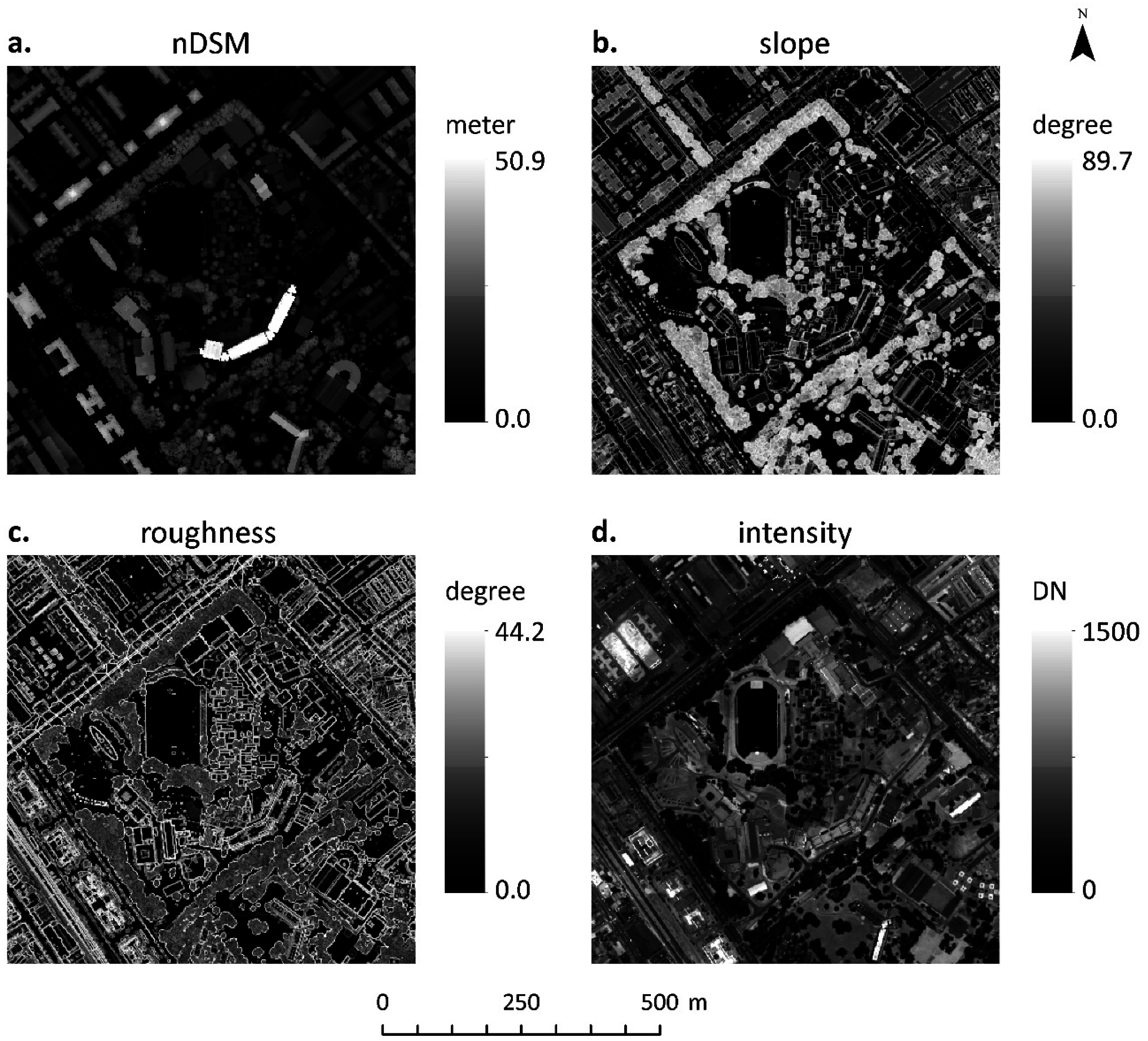
2.1.2. LiDAR and Derived Features

An airborne discrete waveform LiDAR dataset acquired in the winter of 2012 with an average point density of 35 points/m2 after point filtering has been used for this study (LiDAR data provided by the Brussels Regional Informatics Centre). The original extent covering the whole BCR was reduced to that of the hyperspectral image and a 25 cm resolution DSM was extracted using the LAS dataset to raster tool provided in ArcGIS with maximum height values for binning. Linear void filling was used to interpolate caveats in the DSM although these were rare due to the very high LiDAR point density. Subsequently, this DSM was co-registered with the hyperspectral image and resampled to the APEX 2 m resolution. Performing this two-step procedure proved to avoid oversensitivity of the DSM to narrow tall or linear objects present in the urban environment (e.g., antennae and power cables). A normalized DSM or nDSM at 2 m resolution describing the height of pixels above ground level, was produced by subtracting a LiDAR derived Digital Elevation Model (DEM) from the DSM (Figure 2a). From the 25 cm DSM, a slope image was extracted which was in turn used to construct a roughness image (Figure 2b,c). Roughness was acquired by taking the standard deviation of all 25 cm slope pixels located within a 2 m pixel, while slope was calculated by taking the mean value. By means of a procedure similar to that for DSM extraction but with average binning, a LiDAR intensity image was produced (Figure 2d). LiDAR intensity represents the peak amplitude of a backscattered pulse and although this measure is subject to a number of factors, what is mainly important for this study is its correlation with inherent surface brightness and near insensitivity to surface lighting conditions. These are useful characteristics for shadow detection as will be illustrated further on. It has to be noted that due to sensor-to-surface angles of incidence and scattering effects of LiDAR pulses on oblique and very rough surfaces (e.g., canopy), intensity values will not be representative for each material class. Since intensity was delivered in the unitless range of [0, 1500], this range has been rescaled to [0, 1] in order to avoid computational issues during classification and to facilitate comparison with brightness data.

2.1.3. Very High-Resolution Orthophotos and other Ancillary Data
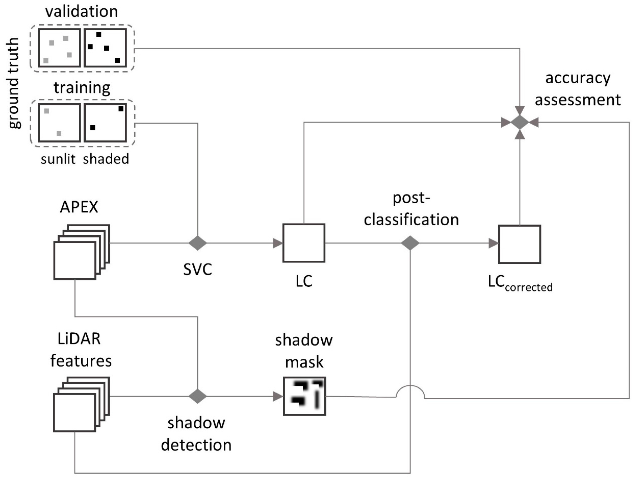
A 2012 winter acquisition RGB-NIR orthophoto with a resolution of 7.5 cm, obtained from the Brussels Regional Informatics Centre, was used as visual reference for the purpose of producing ground truth data over the study area. Ancillary vector datasets from the UrbIS spatial database of Brussels², including water and building shapefiles, have been utilized in this study to improve classification results in post-processing. Google Street View proved to be invaluable in assisting in discriminating different materials at street level, both in and out of shadow. Oblique aerial imagery has also been used to complement the earlier mentioned orthophotos for material discrimination (acquired at http://geoloc.irisnet.be).

2.2. Methodology

2.2.1. Classification Scheme and Sampling Strategy

The complete workflow adopted in this study is depicted in Figure 3. All steps will be explained in further detail over the following paragraphs. The first step in the workflow was the design of a hierarchical classification scheme in which level 2 or the material class level is of particular interest (Table 1). For clarity’s sake, all mention of land cover classes will refer to level 2 unless explicitly stated otherwise. A total of 27 classes were included in the scheme describing some of the most common urban materials (Figure 4) but also some that have only recently been introduced in the urban landscape on a significant scale (e.g., solar panels, reflective hydrocarbon roofing, extensive green roofs). Note that bright roof material is actually a conglomerate of different white PVC, EPDM and other bright hydrocarbon roofing materials as well as bright coatings applied on metal roofs. Attempts to map these as separate classes were unsuccessful due to their spectral similarity and since all these materials serve the same purpose of providing bright impervious roofing, the decision was made to cluster them. Reflective hydrocarbon also mainly consists of PVC and EPDM based roofing materials but here the prevailing colors are gray and to a lesser extent green and red.
For each class, a set of sunlit ground truth polygons with a maximum size of 12 APEX pixels was manually digitized using all available data described above. Except for a limited number of classes, 250–300 spectra were collected per class. In addition, shaded ground truth polygons were digitized for as many material classes as was deemed feasible. Classes with only a marginal occurrence in shadow were excluded and finally 17 out of 27 classes were covered. The amount of digitized shaded polygons is however considerably lower than the amount of sunlit polygons (Table 1). Subsequently, the shaded and sunlit ground truth polygons were each split in training and validation sets based on a 1/3 training and 2/3 validation stratified sampling scheme. Given that the applied SVM classifier is known to retain its ability to generalize even with a limited training sample size, this split ratio was deemed appropriate for this study. The ground truth set of shaded polygons was already limited to start with and the adopted sampling scheme thus ensures a representative accuracy assessment.

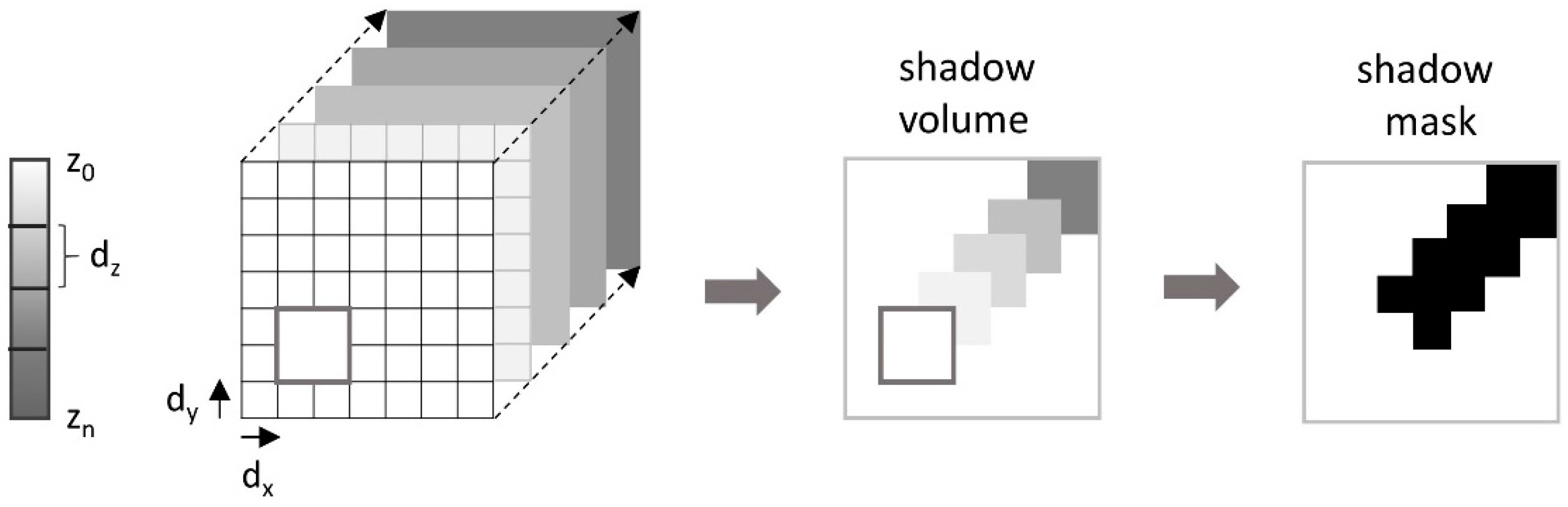
2.2.2. Shadow Detection

A novel shadow detection method is presented here that is inspired by Invariant Color Model shadow detection. The idea of the approach proposed is to use LiDAR derived intensity as an image-external lighting invariant feature, more specifically as a proxy for inherent surface brightness of the APEX image. The first step of the procedure encompasses taking the ratio of LiDAR intensity (scaled to a [0, 1] range) over APEX image brightness. Brightness is calculated simply by taking the average reflectance for each pixel. In this ratio image, high pixel values represent areas where inherent or expected brightness is high compared to the observed brightness in the APEX image. The assumption is made that such areas are affected by cast shadow. In the second step, a manually determined threshold value is applied on the ratio image resulting in a binary shadow mask. A threshold value of 4 was found to cover almost all fully shaded areas without giving rise to overestimation. It should be noted that this shadow detection approach is not suited for identifying areas affected by partial shadow cover or self-shadow. In order to detect those brighter types of shadow, a lower threshold value would be needed but tests indicated that this results in an overestimation of shadow cover on darker sunlit areas.
To allow comparison with other approaches for shadow detection, a machine learning and a geometry-based shadow mask were produced. The former was obtained by training a two class SVM classifier with shaded and sunlit training data, the latter by applying the shadow volume approach proposed by [32] on the 25 cm DSM using solar angles at the time of APEX image acquisition [31,32,33]. The shadow volume approach was implemented by developing a Matlab function that iteratively shifts the DSM in the horizontal direction of cast shadow dx and dy while uniformly subtracting a corresponding decrease in height dz from the DSM. This process continues until the accumulated change in height surpasses the maximal height difference in the DSM or until a predefined number of iterations has been reached that reasonably allows all shadows to be fully projected. A near zenith solar height will cast smaller shadows requiring fewer iterations and vice versa. The resulting shadow volume model can subsequently be converted into a shadow mask simply by subtracting the original DSM from it and converting all positive values to 1 (Figure 5).

2.2.3. Support Vector Classification

Support Vector Machines are a group of non-parametric statistical machine learning methods that are capable of solving complex non-linear classification and regression problems. SVM has proven itself to be robust even when faced with low observations to dimensionality training samples [47]. Not surprisingly, Support Vector Classification has witnessed a drastic growth in popularity over the past decades in many different scientific disciplines, including remote sensing [48,49]. For this study, the imageSVM Classification tools provided by the EnMAP-box software were used to perform SVC [50]. The SVC tools included in EnMAP-box are based on the LIBSVM algorithm. The primary output is a class probability image from which a class image is derived by selecting the class with the highest probability for each pixel [51]. A Support Vector Classification was performed using all sunlit and shaded training data. The output was subjected to a majority filter with a 3 × 3 pixel kernel before validation to smooth out oversensitivity to spectral variations within objects (also referred to as the pepper and salt effect).

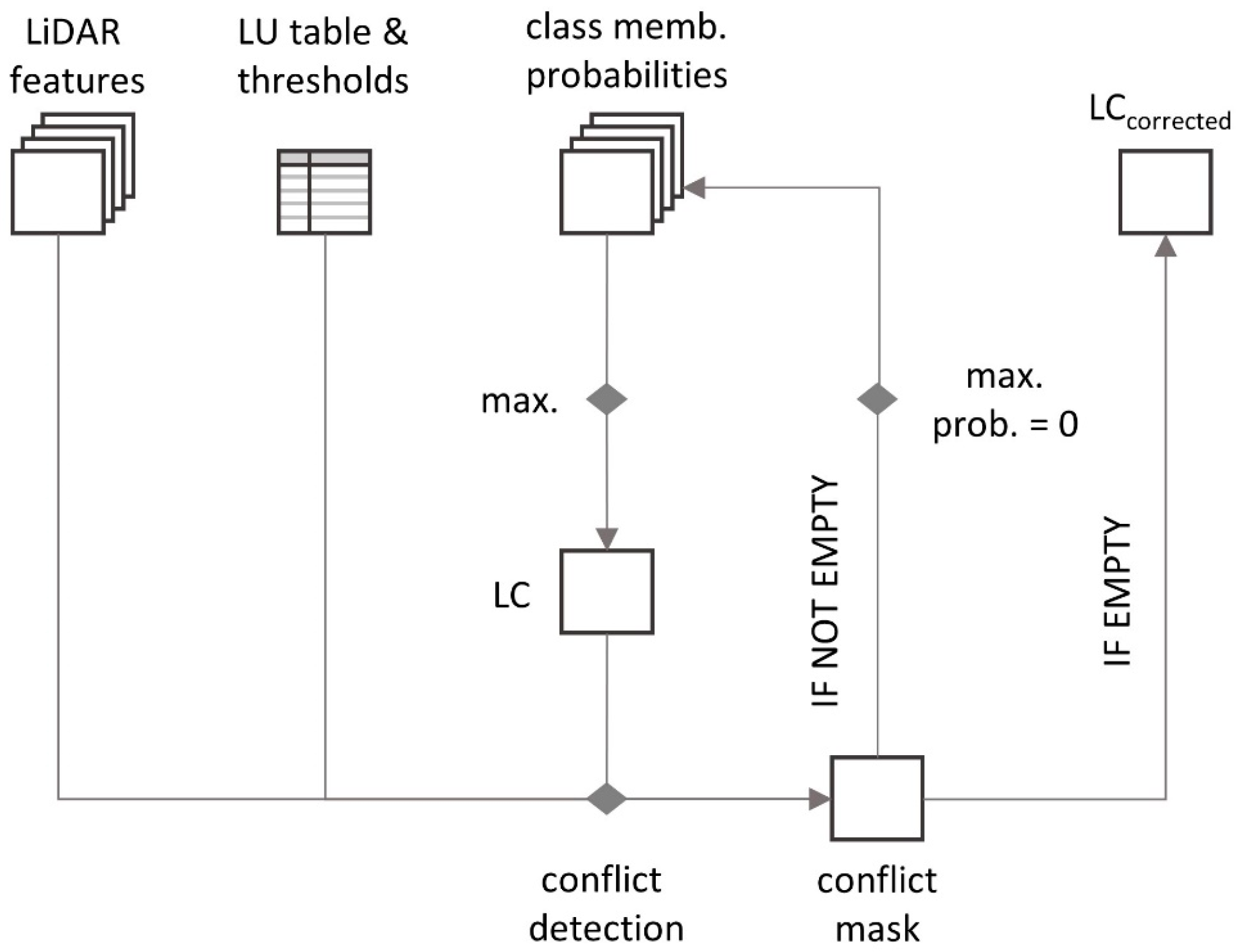
2.2.4. LiDAR Post-Classification Correction

An iterative post-classification correction workflow has been designed and implemented to improve the accuracy of the original SVC (Figure 6 and Code S1 in Supplementary Materials). Essentially, the correction algorithm assesses if the land cover class label assigned by the classifier logically corresponds to the observed spatial characteristics as derived from the LiDAR data. This logic correspondence is implemented by means of a user-defined look-up table in which each land cover class is assigned to a certain range of allowed values of height, slope and roughness. If the observed geometry of a pixel conflicts with any of the ranges of spatial attributes that are associated with the class the pixel has been assigned to, the corresponding class membership probability is set to zero and a new land cover class label is assigned based on the second highest probability. Since the second highest probability will not necessarily provide an acceptable land cover class, this procedure is repeated until no more conflicts are detected for each of the pixels in the image at which point the final corrected land cover image is obtained. For ease of implementation, one threshold value was defined for each LiDAR feature and land cover classes were linked to a range corresponding with all values below or above the threshold. For some combinations of classes and LiDAR features, no thresholds were used (e.g., asphalt can occur both on flat as well as sloped terrain). Based on the distribution of LiDAR feature values for the ground truth data and expert knowledge, the following threshold values were chosen: 0.5 m for height, 15° for slope and 1.8° for roughness. Because roughness is inherently noisy due to spatial errors of LiDAR points, only class assignments for three classes with distinct roughness characteristics (asphalt, concrete and railroad track) were allowed to be corrected based on this feature. In order to account for the presence of asphalt, railroad materials and concrete above street level (as is the case on bridges and viaducts), a vector dataset describing buildings was used. The occurrence of these three materials above 0.5 m was not flagged as a conflict if they occurred on a location that was not a building. Before validation, the output of this correction was also subjected to a majority filter (see above).

2.2.5. Accuracy Assessment

Using an independent set of shaded and sunlit validation polygons as reference data, confusion matrices were constructed for SVM classification, before and after LiDAR post-classification. From these matrices two overall accuracy measures were derived, being Percentage Correctly Classified (PCC) and overall kappa K. Conditional class wise kappas Ki were also calculated. Kappa analysis provides a statistical basis for deciding if the overall or class wise accuracies obtained with different classification approaches significantly differ from each other. The latter can be achieved by calculating the Z-statistic based on the estimates of kappa K1 and K2 and their respective estimated variances var(K1) and var(K2) [52]:
Z = | K 1 K 2 | var ( K 1 ) + var ( K 2 )
Assuming a null hypothesis H0: (K1 − K2) = 0 and alternative hypothesis H1: (K1 − K2) ≠ 0, the null hypothesis is rejected when Z is greater than or equal to a critical value corresponding to a desired level of confidence. In most cases, a critical value of 1.96 is used to assess significant difference corresponding to a 95% confidence level.

3. Results

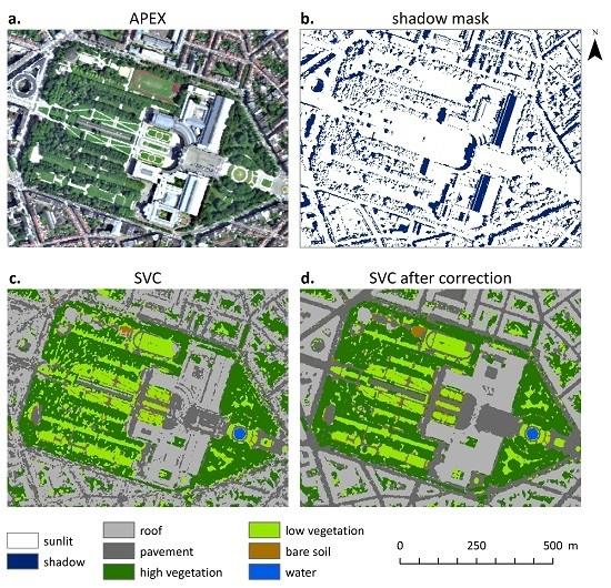
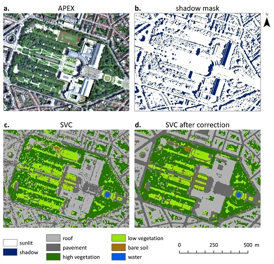
3.1. Shadow Detection

The three selected shadow detection approaches, being Support Vector Classification, shadow volume and intensity-brightness thresholding, were applied on their corresponding input data. In Figure 7, results obtained with the three methods are illustrated for a number of subscenes showing the strengths and weaknesses of each approach. The main drawback of the SVC approach is its susceptibility to false labelling of bright shaded materials as sunlit and dark sunlit materials as shadow. This is clearly illustrated in column 1 of Figure 7 where for SVC dark sunlit roofing is wrongly mapped as shadow while bright roofing located in cast shadow is omitted from the shadow mask. Also, in column 2, parts of shadow cover on ground level are omitted using the SVC approach. Such spectral confusion is avoided by the intensity-brightness and shadow volume approaches but the shadow volume mask does suffer from certain DSM related and APEX mosaicking related issues. Since the APEX flight lines were acquired over a time period of about half an hour not long before solar noon, non-negligible changes in solar azimuth and elevation can be observed in the image. These variations induce considerable errors in some parts of the shadow mask as is highlighted in column 2 of Figure 7. Shadow detection based on DSM height information is furthermore prone to errors caused by long linear objects such as construction cranes and power cables, which is shown in column 3. The weakness of the intensity-brightness approach is related to the effect of LiDAR sensor-to-surface incidence angles on intensity. For materials with rough surfaces or on tilted roofs, a considerable fraction of the inbound pulses will be lost due to scattering, resulting in an underestimation of intensity for those surfaces. The underestimation of self-shadow on oblique roofs is clearly illustrated in column 4 of Figure 7.
A rough quantitative validation of the shadow masks obtained with each approach was accomplished by calculating a PCC based on all shaded validation pixels. Both the SVC and shadow volume approach estimate shadow cover very well and obtain an almost equal PCC of 0.93 and 0.92 respectively. The intensity-brightness approach on the other hand seems to perform less well with a PCC of 0.69. As discussed above, this is the result of a failure to detect brighter partial shadow cover or self-shadow in the set of validation pixels. Nonetheless, an in depth visual analysis of the shadow mask obtained with the brightness-intensity approach (see above) reveals its benefits compared to the other approaches for detecting cast shadow. Based on these findings a hybrid or mixed shadow mask was constructed by combining the intensity and shadow volume masks (bottom row of Figure 7). Ground level shadow was modelled with the intensity mask while rooftop/canopy shadow was defined based on the shadow volume mask. This hybrid approach combines the strengths of both methods and avoids their weaknesses. The final shadow mask was subjected to intensive visual inspection and the same validation procedure was applied as used on the other masks, yielding a superior result with a PCC of 0.99.

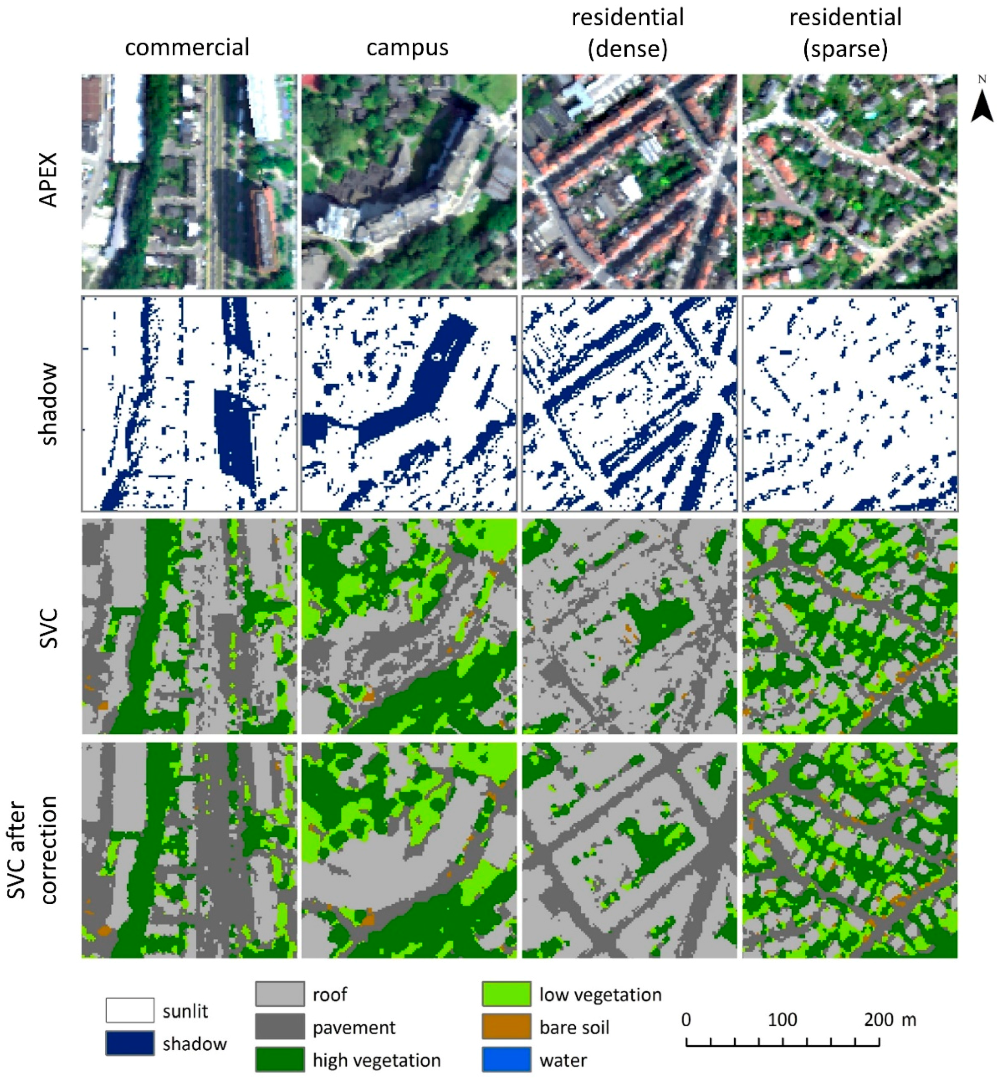
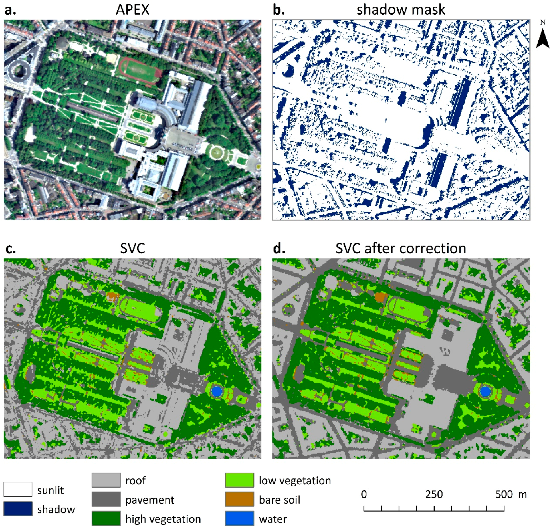
3.2. SVC Land-Cover Mapping

A SVC model was parametrized based on both the sunlit and shaded training data and was subsequently applied to the APEX image. The resulting land-cover classification is illustrated in Figure 8 and Figure 9. In the former four smaller image subsets are shown corresponding to different urban typologies encountered in the image scene: commercial/light industry, university campus, dense residential and sparse residential. In Figure 9, a somewhat larger subset, covering the Cinquantenaire Park and its surroundings, is shown. All maps depict land cover at level 1 of the classification scheme. Accuracy assessment of the land cover mapping output on level 2, based on confusion matrices constructed from the independent set of sunlit and shaded validation polygons, results in a PCC of 0.81 and an overall kappa of 0.80 for sunlit areas and a PCC of 0.67 and overall kappa of 0.65 for shaded areas (Table 2). The difference between PCC and kappa is limited in this case because the high amount of classes included in the classification scheme reduces the impact of chance agreement. As could be expected, the accuracy for shaded areas is considerably lower with a difference of 0.15 in overall kappa.
Visual inspection of the results of Support Vector Classification in Figure 8 and Figure 9 illustrates that there is a considerable amount of confusion present in this output. In the campus and dense residential areas of Figure 8, one can clearly observe that the presence of shadow has a considerable impact on mapping results. Even sunlit pavement and roof classes are not well identified in multiple areas of the commercial, campus and dense residential subsets. Notably, the sunlit part of the North-South oriented boulevard in the commercial subscene indicates a very high degree of confusion between roof and pavement classes. With exception of the sparse residential subscene, numerous examples of pavement–roof confusion can be found in the different subscenes shown in Figure 8. Similar effects can be observed in the Cinquantenaire subset (Figure 9) and here an intermixing between low and high vegetation can also be seen, especially in the shaded parts of canopy. Mapping output seems to be quite noisy, making it difficult to identify the structures present in the urban environment well. The sparse residential subset however seems to produce reasonably good results based on spectral information only.
Also, accuracies at class level for sunlit and shaded areas have been estimated by means of conditional kappas. These results can be found in the SVC column of Table 3 and Table 4, respectively. To ease interpretation of these extensive tables, summarizing graphs have been provided. In Figure 10, the class-wise accuracy profile of the SVC mapping output (before correction) is illustrated separately for sunlit and shaded areas. In sunlit areas, the classifier performs reasonably well up to very well for most classes. Only four out of 27 land-cover classes have accuracies lower than 0.7 while the other 23 classes consequently have kappas higher than or equal to 0.7, 11 classes even have conditional kappa values of more than 0.9. For the shaded part of the classification, the classes with poor to very poor conditional kappas (<0.7) outnumber the classes with good to very good kappas (≥0.7). A total of six classes out of 17 have very poor kappas (<0.5), underlining the difficulty of urban material mapping in shadow.

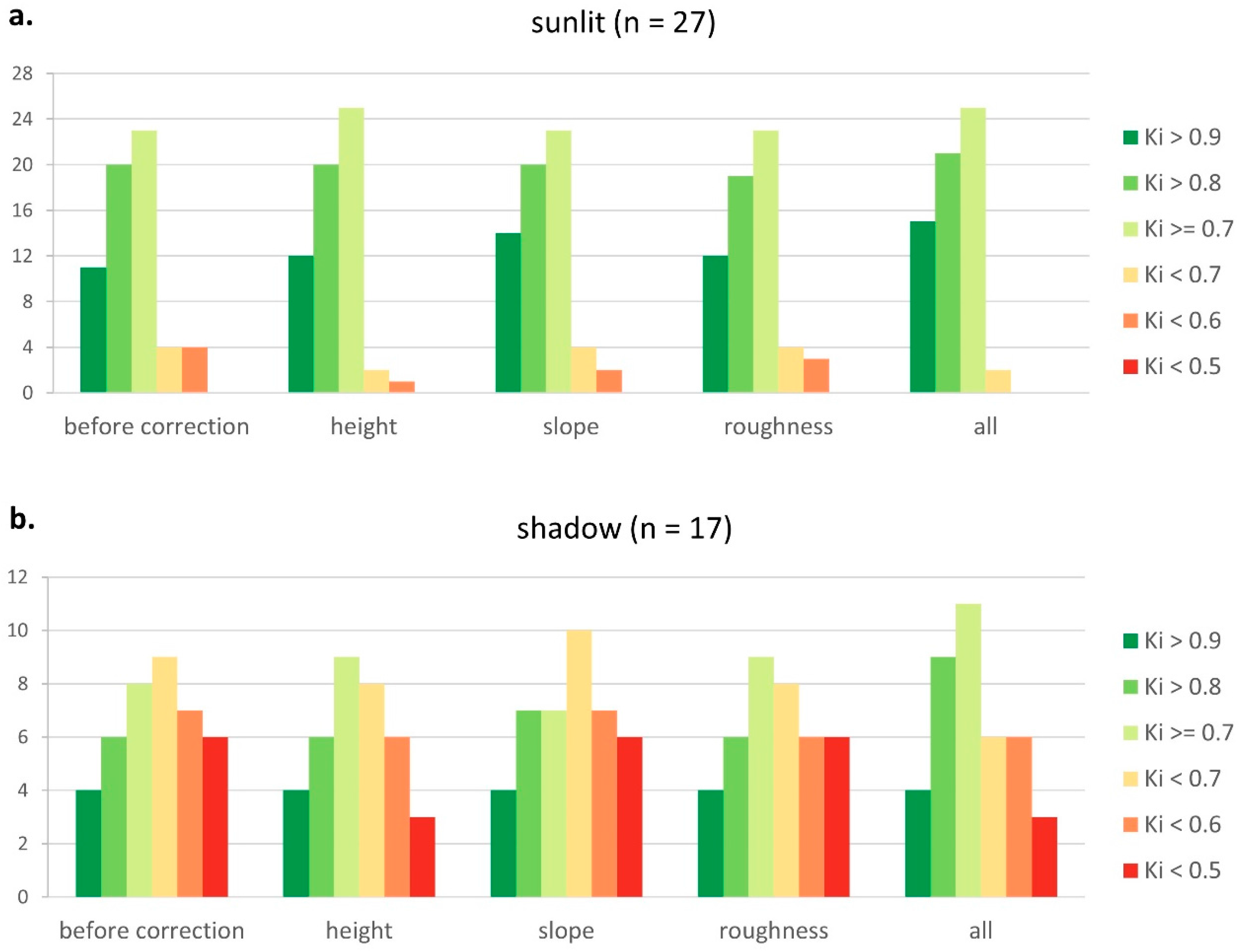
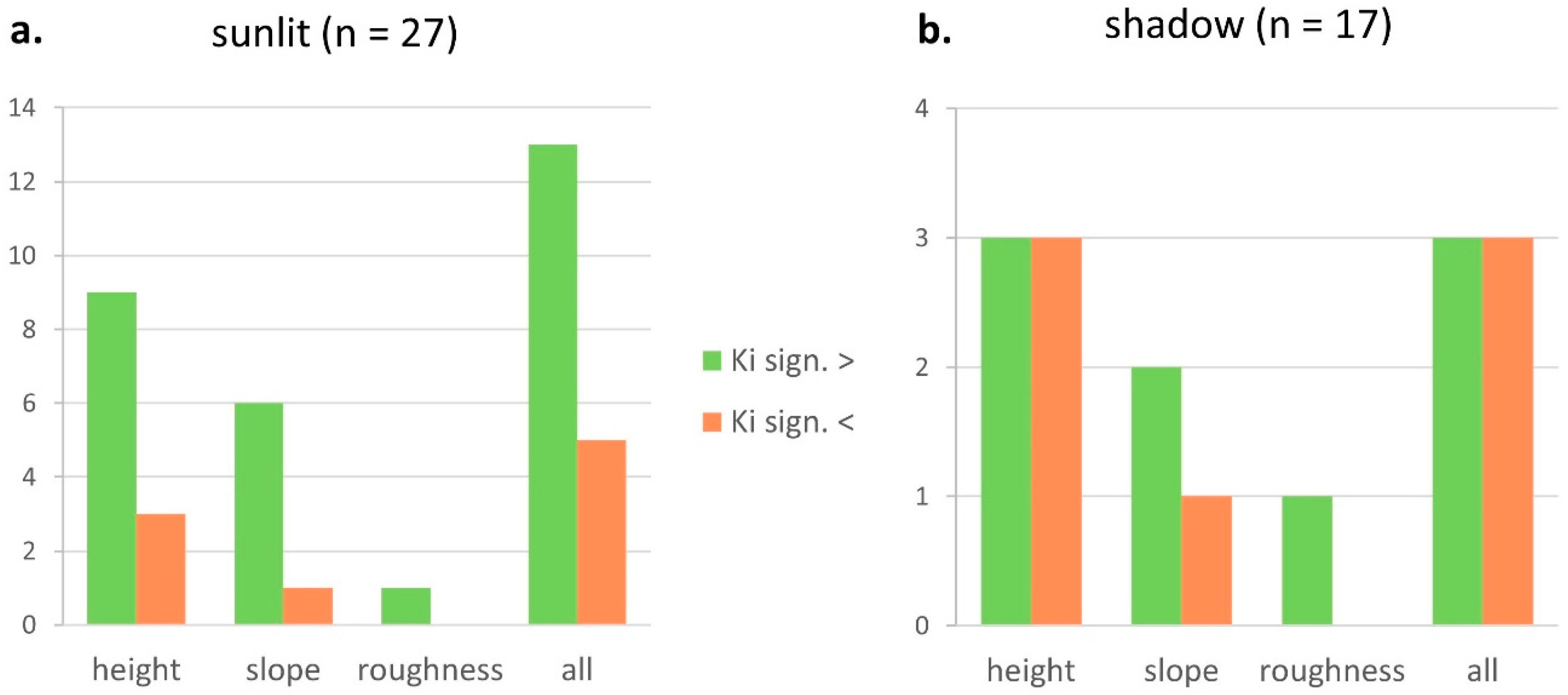
3.3. LiDAR Post-Classification Correction

As explained in Section 2.2.4, SVC class membership probabilities, LiDAR features (height, slope and roughness) as well as user defined look-up tables and threshold values were entered in the iterative post-classification correction algorithm. Corrections were run for each separate LiDAR feature and for the combination of them all in order to assess their relative impacts on mapping accuracy. Subsets of the corrected land-cover maps are included in Figure 8 and Figure 9. Each LiDAR correction was validated using the same procedure as above. The overall results of these validations are included in Table 2. Correction with height clearly has the most positive impact on accuracies for both sunlit and shaded surfaces, resulting in a significant increase in overall kappa from 0.80 to 0.84 and from 0.65 to 0.69, respectively. Correction based on slope leads to a significant increase in overall kappa for sunlit areas from 0.80 to 0.83. In terms of overall kappa, no significant improvement is achieved with a correction based on roughness, neither for sunlit areas nor for shaded areas. Using all features together produces the highest accuracies, with an overall kappa of 0.87 for sunlit pixels and 0.69 for shaded pixels.
When looking at results obtained at class level (Table 3 and Table 4), correction with height and slope results in an increase of conditional kappa for some classes, but in a decrease in kappa for other. Roughness does not seem to have much impact on classification accuracy at class level, except for sunlit railroad track and for shaded high vegetation, which both show a substantial increase in conditional kappa. Figure 10 shows class-based accuracy profiles for each type of correction, indicating the number of classes reaching a certain level of accuracy, based on conditional kappas (Table 3 and Table 4), while Figure 11 depicts the number of classes with significantly higher and lower conditional kappa’s after correction, compared to SVC based on spectral data only. When comparing accuracy profiles before and after correction (Figure 10) one can see that the amount of classes with good (≥0.7) to very good (>0.9) kappas tends to increase while the amount of classes with poor (<0.7) to very poor (< 0.5) kappas decreases. In sunlit areas (Figure 10a), the improvement is most marked when using height or slope as a feature for correction. The impact of roughness is clearly limited. Best results are obtained when using all features together. In terms of the number of classes for which the kappa value significantly improves (Figure 11a), height correction clearly has the strongest impact, followed by slope correction, while the impact of roughness is limited. When using all features for correction, the highest gain is reached, although it must be mentioned that correction also reduces the accuracy for several classes (for details see Table 3). LiDAR correction yields less positive results for shaded pixels (Figure 10b and Figure 11b). Although correction undeniably improves overall accuracy, an increase in accuracy for some classes seems to be counterbalanced by a decrease in accuracy for other.
Comparison of the SVC and post-classification land-cover maps in Figure 8 and Figure 9 clearly indicates that synergistic use of machine learning classification of hyperspectral imagery and LiDAR post-classification yields an improved mapping result. Even though the level 1 maps shown do not display the full extent of between-material class confusion, especially in shadow, LiDAR correction undeniably allows to capture the typical morphological characteristics of urban areas better compared to mapping with only APEX data. Both in sunlit and shaded regions mapping results are less noisy and one can clearly identify the building block and street patterns present in the subscenes. Besides clearing out numerous cases of pavement-roof confusion, on Figure 9 it can be seen that shadow located in canopy, before often wrongly classified as low vegetation, is corrected in the final map. Improvements are limited for the sparse residential subset which is already mapped rather well using spectral data only.

4. Discussion

4.1. Shadow Detection

Two established shadow detection approaches were applied in this study: an image-based SVM machine learning approach and a LiDAR-based geometric model approach. Both approaches produce good results but show different strengths and weaknesses. The SVM approach is better equipped to handle self-shadow and partial shadow cover but suffers from spectral confusion between dark materials and shadow. The geometric approach is not affected by spectral confusion but fails to capture partial shadow cover. It also leads to errors induced by projection of linear objects and proves to be sensitive to small differences in solar angle caused by mosaicking data obtained from consecutive flight lines. Based on these observations a new hybrid shadow detection method has been proposed that uses both image and LiDAR data and combines intensity-brightness thresholding with DSM-derived shadow mask detection. The approach has been shown to benefit from the strength of both methods, while compensating for their respective weaknesses.
The hybrid shadow mask allowed producing an estimate of the relative shadow cover in the complete image scene which amounts to 17.64%, implying that the image is for nearly one fifth covered by shadow. This highlights the importance of paying particular attention to the presence of shadow in developing approaches for mapping of urban scenes, as well as in assessing the accuracy of the mapping methods used. The hybrid shadow mask detection approach proposed in this study is relatively easy to apply, and may be very useful as a preprocessing step prior to image classification, to facilitate the collection of ground truth data needed for both training and validation of supervised image classification approaches incorporating spectra for both shaded and sunlit areas. Moreover, if validation is performed separately for sunlit and shadow areas, the shadow mask is also useful to spatially identify regions characterized by lower mapping accuracies due to the presence of shadow, and to demonstrate the impact of improvements induced by post-processing in both shaded and non-shaded areas, as has been clearly demonstrated in this study. Use of a shadow mask in combination with confusion matrices defined separately for shaded and sunlit areas also opens possibilities for spatially explicit modelling of image classification uncertainty (at pixel level), thereby acknowledging differences in the performance of the classifier within and outside shaded areas.

4.2. SVC Land-Cover Mapping

Results obtained with SVC, based on spectral information only, reveal that: (1) overall accuracies are much higher for sunlit than for shaded areas; (2) a considerable degree of confusion occurs between certain roof and pavement materials, particularly in shaded areas.
As shown in Table 3, most sunlit classes perform reasonably to very well in terms of mapping accuracy. Sunlit classes with poor conditional kappas (kappa < 0.7) entail bright roof material, cobblestone, concrete and dark shingle. The confusion matrix for sunlit areas (see Table S1 in Supplementary Materials) reveals a number of spectral similarities between these and other sunlit classes. The most significant confusion occurs between bright roof material, concrete and to some extent bare soil and between dark shingle, bitumen and hydrocarbon roofing. Also bitumen, dark shingle and asphalt are to some extent confused by the SVM classifier, which could have been expected based on the very similar and relatively unpronounced spectral features of these materials (Figure 4a). Similar material compositions and/or effects related to material condition (e.g., degraded asphalt or bitumen exhibiting a higher brightness) have a negative impact on land-cover mapping accuracy, despite the high spectral resolution of the APEX image.
Class-specific conditional kappas in Table 4 provide a clearer picture of the specific strengths and weaknesses of the SVC in the shaded part of the image scene. A number of classes seem to perform relatively well in shadow (kappa > 0.8), including fiber cement and gray metal roofs as well as railroad track, bright gravel, red gravel and low vegetation. Pavement materials that perform very poorly (kappa < 0.5) include asphalt, concrete, cobblestone as well as bitumen, dark shingle, high vegetation and red ceramic tile roofs. At least four factors can help explain why a material can be mapped accurately or not in shadow cover: (1) the uniqueness of the material’s spectral signature (also applies outside shadow); (2) the occurrence of the material’s characteristic spectral features inside parts of the spectrum disturbed by shadow; (3) the amplitude of these features (also applies outside shadow); and (4) the inherent brightness of the material that can often be related to (3) and vice versa.
The confusion matrix of the SVC for shaded areas (see Table S2 in Supplementary Materials) reveals that there is a great deal of spectral confusion between pavement classes such as concrete and asphalt. Figure 4a suggests that separability of sunlit concrete and asphalt is possibly due to brightness differences even though the signatures of these two material classes share similar spectral features. In shadow (Figure 4b), this brightness difference largely disappears, explaining the high degree of confusion and suboptimal accuracies. In addition, there is a great deal of shadow induced roof–pavement confusion, especially for asphalt–bitumen and cobblestone–red ceramic tile. This confusion could be expected, and also occurs, be it to a smaller extent, in sunlit areas as these classes share similar material compositions. Inherently bright classes such as bright roof materials or bright gravel seem to suffer less from the effect of shadow on spectral response (Figure 4b).

4.3. LiDAR Post-Classification Correction

Three observations can be made based on the results obtained: (1) in order of decreasing importance height, slope and roughness LiDAR features contribute to an improved mapping output after LiDAR-based post-classification; (2) when used together the different features seem to complement each other by improving accuracies of different material classes and compensating for some of the decreases in conditional kappa observed when LiDAR features are used separately; (3) improvements through post-classification are limited in shaded areas.
A few remarkable cases of confusion endure in sunlit regions even after correction (see Table S3 in Supplementary Materials), including cobblestone-asphalt, bright roof materials-gray metal-paved roof and bare soil-various materials with a mineral component. The latter is a classic problem encountered in urban remote sensing that is apparently very difficult to eliminate fully even when using hyperspectral information. A detailed look at the error matrix for shaded areas after post-classification correction (see Table S4 in Supplementary Materials) points out that some low accuracy shaded pavement classes are confused considerably. The same holds for some shaded roof classes. This finding indicates that some degree of thematic aggregation may be needed to allow accuracies in shaded areas to reach acceptable levels. Accuracy assessment of the final land-cover map on level 1 yields overall kappas of respectively 0.96 and 0.95 for sunlit and shaded areas, but this relatively limited level of thematic detail may have little added value for urban applications that require material (condition) information.
Based on the observations made above, some final considerations concerning the LiDAR correction model are in place. For one it became clear that with each included LiDAR feature a trade-off between increases in accuracy for certain material classes and decreases for other classes occurred (Table 3 and Table 4). The correction model starts from the SVC land-cover class membership probabilities from which the highest value is removed for each pixel when a conflict between the land cover class the pixel is assigned to and the allowed ranges of LiDAR feature values for that class occurs. The basic assumption underlying this approach is that class probability ranking allows the classifier to identify the class that is actually present in a pixel after all classes with higher probabilities flagged by conflict have been removed. This assumption will of course not be valid for all wrongly classified pixels and so LiDAR correction will induce some commission errors on other classes. As long as the correction balance remains positive, such losses in accuracy can be justified. Secondly, combining different LiDAR features can lead to a compensation of decreases in class accuracies prompted by the use of separate LiDAR features. Including multiple LiDAR features increases the detection of possible conflicts and thus reduces the chance of accepting incorrect classes with high class membership probabilities. Thirdly, the overall poorer response of shaded pixels to LiDAR post-classification can be explained by spectral limitations. Besides having a very low brightness, signatures of shaded pixels are also disturbed by radiance originating from the immediate environment and the atmosphere. These combined effects result in less interpretable signatures and thus less reliable modelled class membership probabilities. Clearly this has an impact on the effectiveness of the adopted post-classification approach but nonetheless significant improvements in overall accuracy are still achieved.

5. Conclusions

Hitherto, few studies have looked into the potential of combining airborne imaging spectroscopy and laser altimetry for managing particular difficulties of urban land-cover mapping. Especially the topic of shadow remains underexplored in this setting. In the study presented here, an urban land-cover mapping workflow was developed for synergistic use of an APEX hyperspectral image and a discrete return LiDAR dataset and applied on an urban transect covering part of the Brussels Capital Region. For the purpose of investigating the effect of shadow on classification performance, separate shaded and sunlit ground truth polygons were digitized. A novel shadow detection method has been proposed based on applying thresholding on a normalized LiDAR intensity over APEX brightness ratio image. This approach was compared to a classification-based approach and LiDAR DSM shadow volume detection. The results revealed that intensity-brightness thresholding, as proposed in this study, and DSM-derived shadow mask detection each display unique strengths and weaknesses and that combining both approaches results in a highly accurate shadow mask reflecting the strengths of both methods.
Support Vector Classification with both shaded and sunlit training data followed by a majority filtering yielded respective overall kappas of 0.65 and 0.80 for shaded and sunlit regions for a classification distinguishing 27 land-cover types in sunlit areas and 17 land-cover types in shaded areas. Accuracy assessment on class level revealed that the mapping output suffered considerably from confusion induced by strong within-class spectral heterogeneity and spectral similarity between classes with similar material compositions. The output of SVC mapping was corrected through an iterative post-classification workflow using SVC class membership probabilities and LiDAR features as an input. The use of different features, being height, slope and roughness, was tested separately and combined in the correction workflow. All separate features significantly contributed to a better outcome, either overall, on class level or both, but primarily height information and secondarily slope information had the highest impact on accuracies. The overall kappas of the final correction with all LiDAR features amounted to 0.87 and 0.69 for sunlit and shaded areas, respectively. Class-wise accuracies confirmed that shaded pixels respond less positively to the proposed correction due to their unreliable SVC class membership probabilities. Despite the satisfactory results achieved for sunlit pixels, accuracies obtained for shaded pixels remained suboptimal after correction. Taking into account the loss of spectral information due to shading, in addition to the challenge of mapping urban materials even under optimal conditions, improvements obtained in shaded areas are still significant. The result of this research underlines the potential, and perhaps even the necessity of combining hyperspectral imagery and LiDAR for thematically detailed urban land-cover mapping.

Supplementary Materials

The following are available online at www.mdpi.com/2072-4292/8/10/787/s1. Code S1: Matlab code developed for performing iterative LiDAR correction in post-classification based on LiDAR features and SVC class membership probabilities. Table S1: confusion matrix sunlit validation SVC, Table S2: confusion matrix shaded validation SVC, Table S3: confusion matrix sunlit validation SVC after post-classification correction with all LiDAR features, Table S4: confusion matrix shaded validation SVC after post-classification correction with all LiDAR features.

Acknowledgments

The research pertaining to these results received financial aid from the Federal Science Policy (BELSPO) according to the agreement of subsidy no SR/00/307 (UrbanEARS), SR/67/167 (BELAIR 2013), SR/XX/170 (BELAIR SONIA) and SR/03/333 (BELAIR SONIA 2015). In addition we acknowledge the imagery, spatial datasets and support provided by the Brussels Regional Informatics Centre (BRIC).

Author Contributions

F.P. and F.C. conceived and designed the experiments, F.P. performed the experiments, analyzed the results, and wrote the initial draft of the paper, F.C. supervised the research and contributed to improving the manuscript prior to submission, F.P. and F.C. prepared the final version of the manuscript taking into account the comments made by the reviewers.

Conflicts of Interest

The authors declare no conflict of interest.

References

  1. Rashed, T.; Jürgens, C. Remote Sensing of Urban and Suburban Areas; Springer: London, UK, 2010. [Google Scholar]
  2. Ben-Dor, E. Imaging spectrometry for urban applications. In Imaging Spectrometry: Basic Principles and Prospective Applications; Van Der Meer, F.D., De Jong, S.M., Eds.; Kluwer Academic Publishers: Dordrecht, The Netherland, 2001; pp. 243–281. [Google Scholar]
  3. Roberts, D.A.; Herold, M. Imaging spectroscopy of urban materials. In Infrared Spectroscopy in Geochemistry, Exploration and Remote Sensing; King, P., Ramsey, M.S., Swayze, G., Eds.; Mineral Association of Canada: Ottawa, ON, Canada, 2004; pp. 155–181. [Google Scholar]
  4. Xian, G.Z. Remote Sensing Applications for the Urban Environment; CRC Press, Taylor & Francis Group: Boca Raton, FL, USA, 2015. [Google Scholar]
  5. Ben-Dor, E. Quantitative Remote Sensing of Soil Properties. Adv. Agron. 2002, 75, 173–243. [Google Scholar]
  6. Wu, C. Normalized spectral mixture analysis for monitoring urban composition using ETM+ imagery. Remote Sens. Environ. 2004, 93, 480–492. [Google Scholar] [CrossRef]
  7. Deng, Y.; Wu, C.; Li, M.; Chen, R. RNDSI: A ratio normalized difference soil index for remote sensing of urban/suburban environments. Int. J. Appl. Earth Obs. Geoinf. 2015, 39, 40–48. [Google Scholar] [CrossRef]
  8. Herold, M.; Schiefer, S.; Hostert, P.; Roberts, D.A. Applying imaging spectrometry in urban areas. In Urban Remote Sensing; Weng, Q., Quattrochi, D.A., Eds.; CRC Press, Taylor & Francis Group: Boca Raton, FL, USA, 2007; pp. 137–161. [Google Scholar]
  9. Yan, W.Y.; Shaker, A.; El-Ashmawy, N. Urban land cover classification using airborne LiDAR data: A review. Remote Sens. Environ. 2015, 158, 295–310. [Google Scholar] [CrossRef]
  10. Raychaudhuri, B. Imaging spectroscopy: Origin and future trends. Appl. Spectrosc. Rev. 2016, 51, 23–35. [Google Scholar] [CrossRef]
  11. Hardin, P.; Hardin, A. Hyperspectral remote sensing of urban areas. Geogr. Compass 2013, 1, 7–21. [Google Scholar] [CrossRef]
  12. Brubaker, K.M.; Myers, W.L.; Drohan, P.J.; Miller, D.A.; Boyer, E.W. The Use of LiDAR Terrain data in characterizing surface roughness and microtopography. Appl. Environ. Soil Sci. 2013, 2013, 1–13. [Google Scholar] [CrossRef]
  13. Song, J.; Han, S.; Yu, K.; Kim, Y. Assessing the possibility of land-cover classification using LiDAR intensity data. Int. Arch. Photogramm. Remote Sens. Spat. Inf. Sci. 2002, 34, 259–262. [Google Scholar]
  14. Mallet, C.; Bretar, F.; Roux, M.; Soergel, U.; Heipke, C. Relevance assessment of full-waveform LiDAR data for urban area classification. ISPRS J. Photogramm. Remote Sens. 2011, 66, S71–S84. [Google Scholar] [CrossRef]
  15. Mallet, C.; Bretar, F. Full-waveform topographic LiDAR: State-of-the-art. ISPRS J. Photogramm. Remote Sens. 2009, 64, 1–16. [Google Scholar] [CrossRef]
  16. Khodadadzadeh, M.; Member, S.; Li, J.; Prasad, S.; Member, S. Fusion of hyperspectral and LiDAR remote sensing data using multiple feature learning. J. Sel. Top. Appl. Earth Obs. Remote Sens. 2015, 8, 1–13. [Google Scholar] [CrossRef]
  17. Ghamisi, P.; Benediktsson, J.A.; Phinn, S. Land-cover classification using both hyperspectral and LiDAR data. Int. J. Image Data Fusion 2015, 6, 189–215. [Google Scholar] [CrossRef]
  18. Heiden, U.; Heldens, W.; Roessner, S.; Segl, K.; Esch, T.; Mueller, A. Urban structure type characterization using hyperspectral remote sensing and height information. Landsc. Urban Plan. 2012, 105, 361–375. [Google Scholar] [CrossRef]
  19. Brook, A.; Ben-Dor, E.; Richter, R. Modelling and monitoring urban built environment via multi-source integrated and fused remote sensing data. Int. J. Image Data Fusion 2011, 9832, 1–31. [Google Scholar] [CrossRef]
  20. Alonzo, M.; Bookhagen, B.; Roberts, D.A. Urban tree species mapping using hyperspectral and LiDAR data fusion. Remote Sens. Environ. 2014, 148, 70–83. [Google Scholar] [CrossRef]
  21. Huang, X.; Zhang, L.; Gong, W. Information fusion of aerial images and LiDAR data in urban areas: Vector-stacking, re-classification and post-processing approaches. Int. J. Remote Sens. 2011, 32, 69–84. [Google Scholar] [CrossRef]
  22. Gamba, P. Image and data fusion in remote sensing of urban areas: Status issues and research trends. Int. J. Image Data Fusion 2013, 5, 2–12. [Google Scholar] [CrossRef]
  23. Gamba, P.; Lisini, G.; Tomas, L.; Almeida, C.; Fonseca, L. Joint VHR-LIDAR classification framework in urban areas using a priori knowledge and post processing shape optimization. In Proceedings of the 2011 Joint Urban Remote Sensing Event (JURSE), Munich, Germany, 11–13 April 2011; pp. 93–96.
  24. Van de Voorde, T.; De Genst, W.; Canters, F. Improving pixel-based VHR land-cover classifications of urban areas with post-classification techniques. Photogramm. Eng. Remote Sens. 2007, 73, 1017–1027. [Google Scholar]
  25. Dare, P.M. Shadow Analysis in High-Resolution Satellite Imagery of Urban Areas. Photogramm. Eng. Remote Sens. 2005, 71, 169–177. [Google Scholar] [CrossRef]
  26. Arévalo, V.; González, J.; Ambrosio, G. Shadow detection in colour high-resolution satellite images. Int. J. Remote Sens. 2008, 29, 1945–1963. [Google Scholar] [CrossRef]
  27. Adler-golden, S.M.; Levine, R.Y.; Matthew, M.W.; Richtsmeier, S.C.; Bernstein, L.S.; Gruninger, J.; Felde, G.; Hoke, M.; Anderson, G.; Ratkowski, A. Shadow-Insensitive material detection/classification with atmospherically corrected hyperspectral imagery. Proc. SPIE 2001. [Google Scholar] [CrossRef]
  28. Adeline, K.R.M.; Chen, M.; Briottet, X.; Pang, S.K.; Paparoditis, N. Shadow detection in very high spatial resolution aerial images: A comparative study. ISPRS J. Photogramm. Remote Sens. 2013, 80, 21–38. [Google Scholar] [CrossRef]
  29. Shahtahmassebi, A.; Yang, N.; Wang, K.; Moore, N.; Shen, Z. Review of shadow detection and de-shadowing methods in remote sensing. Chinese Geogr. Sci. 2013, 23, 403–420. [Google Scholar] [CrossRef]
  30. Tolt, G.; Shimoni, M.; Ahlberg, J. A shadow detection method for remote sensing images using VHR hyperspectral and LiDAR data. In Proceedings of the 2011 IEEE International Geoscience and Remote Sensing Symposium (IGARSS), Vancouver, BC, Canada, 24–29 July 2011; pp. 4423–4426.
  31. Ratti, C.; Richens, P. Raster analysis of urban form. Environ. Plan. B Plan. Des. 2004, 31, 297–309. [Google Scholar] [CrossRef]
  32. Richens, P. Image processing for urban scale environmental modelling. In Proceedings of the 5th Intemational IBPSA Conference: Building Simulation 97, Prague, Czech Republic, 1 Janunary 1997.
  33. Morello, E.; Ratti, C. Sunscapes: “Solar envelopes” and the analysis of urban DEMs. Comput. Environ. Urban Syst. 2009, 33, 26–34. [Google Scholar] [CrossRef]
  34. Tsai, V.J.D. A comparative study on shadow compensation of color aerial images in invariant color models. IEEE Trans. Geosci. Remote Sens. 2006, 44, 1661–1671. [Google Scholar] [CrossRef]
  35. Lorenzi, L.; Melgani, F.; Mercier, G. A complete processing chain for shadow detection and reconstruction in VHR images. IEEE Trans. Geosci. Remote Sens. 2012, 50, 3440–3452. [Google Scholar] [CrossRef]
  36. Ashton, E.; Wemett, B.; Leathers, R.; Downes, T. A novel method for illumination suppression in hyperspectral images. Proc. SPIE 2008. [Google Scholar] [CrossRef]
  37. Friman, O.; Tolt, G.; Ahlberg, J. Illumination and shadow compensation of hyperspectral images using a digital surface model and non-linear least squares estimation. Proc. SPIE 2011. [Google Scholar] [CrossRef]
  38. Wu, S.T.; Hsieh, Y.T.; Chen, C.T.; Chen, J.C. A Comparison of 4 shadow compensation techniques for land cover classification of shaded areas from high radiometric resolution aerial images. Can. J. Remote Sens. 2014, 40, 315–326. [Google Scholar] [CrossRef]
  39. Itten, K.I.; Dell’Endice, F.; Hueni, A.; Kneubühler, M.; Schläpfer, D.; Odermatt, D.; Seidel, F.; Huber, S.; Schopfer, J.; Kellenberger, T.; et al. APEX—the hyperspectral ESA airborne prism experiment. Sensors 2008, 8, 6235–6259. [Google Scholar] [CrossRef] [Green Version]
  40. Schaepman, M.E.; Jehle, M.; Hueni, A.; D’Odorico, P.; Damm, A.; Weyermann, J.; Schneider, F.D.; Laurent, V.; Popp, C.; Seidel, F.C.; et al. Advanced radiometry measurements and earth science applications with the Airborne Prism Experiment (APEX). Remote Sens. Environ. 2015, 158, 207–219. [Google Scholar] [CrossRef]
  41. De Haan, J.F.; Hovenier, J.W.; Kokke, J.M.M.; van Stokkom, H.T.C. Removal of atmospheric influences on satellite-borne imagery: A radiative transfer approach. Remote Sens. Environ. 1991, 37, 1–21. [Google Scholar] [CrossRef]
  42. Sterckx, S.; Vreys, K.; Biesemans, J.; Iordache, M.D.; Bertels, L.; Meuleman, K. Atmospheric correction of APEX hyperspectral data. Misc. Geogr. 2016, 20, 16–20. [Google Scholar] [CrossRef]
  43. Vreys, K.; Iordache, M.-D.; Bomans, B.; Meuleman, K. Data acquisition with the APEX hyperspectral sensor. Misc. Geogr. 2016, 20, 5–10. [Google Scholar] [CrossRef]
  44. Vreys, K.; Iordache, M.-D.; Biesemans, J.; Meuleman, K. Geometric correction of APEX hyperspectral data. Misc. Geogr. 2016, 20, 11–15. [Google Scholar] [CrossRef]
  45. Cariou, C.; Chehdi, K.; Le Moan, S. BandClust: An unsupervised band reduction method for hyperspectral remote sensing. IEEE Geosci. Remote Sens. Lett. 2011, 8, 565–569. [Google Scholar] [CrossRef]
  46. Demarchi, L.; Canters, F.; Cariou, C.; Licciardi, G.; Chan, J.C.W. Assessing the performance of two unsupervised dimensionality reduction techniques on hyperspectral APEX data for high resolution urban land-cover mapping. ISPRS J. Photogramm. Remote Sens. 2014, 87, 166–179. [Google Scholar] [CrossRef]
  47. Chi, M.; Feng, R.; Bruzzone, L. Classification of hyperspectral remote-sensing data with primal SVM for small-sized training dataset problem. Adv. Sp. Res. 2008, 41, 1793–1799. [Google Scholar] [CrossRef]
  48. Mammone, A.; Turchi, M.; Cristianini, N. Support vector machines. Wiley Interdiscip. Rev. Comput. Stat. 2009, 1, 283–289. [Google Scholar] [CrossRef]
  49. Mountrakis, G.; Im, J.; Ogole, C. Support vector machines in remote sensing: A review. ISPRS J. Photogramm. Remote Sens. 2011, 66, 247–259. [Google Scholar] [CrossRef]
  50. Van der Linden, S.; Rabe, A.; Held, M.; Jakimow, B.; Leitão, P.J.; Okujeni, A.; Schwieder, M.; Suess, S.; Hostert, P. The EnMAP-box-A toolbox and application programming interface for EnMAP data processing. Remote Sens. 2015, 7, 11249–11266. [Google Scholar] [CrossRef]
  51. Chang, C.-C.; Lin, C.J. Libsvm. ACM Trans. Intell. Syst. Technol. 2011, 2, 1–27. [Google Scholar] [CrossRef]
  52. Congalton, R.G.; Green, K. Assessing the Accuracy of Remotely Sensed Data: Principles and Practices, 2nd ed.; CRC Press, Taylor & Francis Group: Boca Raton, FL, USA, 2009. [Google Scholar]
Figure 1. (a) RGB-image (R = band 36, G = band 18 and B = band 5) of the 2013 APEX image covering the Eastern part of the Brussel Capital Region and (b) inset map for VUB university campus. Annotations in (b) refer to material spectra (see below).
Remotesensing 08 00787 g001
Figure 2. LiDAR features used in this research illustrated for the VUB university campus with (a) normalized DSM; (b) slope; (c) roughness and (d) intensity (expressed in uncalibrated Digital Numbers (DN)).
Remotesensing 08 00787 g002
Figure 3. Flowchart outlining the workflow implemented in this research.
Remotesensing 08 00787 g003
Figure 4. Examples of different material spectra sampled from the APEX image and included in the set of ground truth data with (a) sunlit spectra and (b) shaded spectra. Notice that the materials have been annotated in Figure 1b.
Remotesensing 08 00787 g004
Figure 5. Overview of the DSM model-based shadow detection approach, in this paper referred to as shadow volume approach.
Remotesensing 08 00787 g005
Figure 6. Detailed workflow of the iterative LiDAR post-classification correction used in this research.
Remotesensing 08 00787 g006
Figure 7. Results of the four shadow detection approaches (detected shadow shown in purple) applied in this research for a selection of APEX subsets illustrating strengths and weaknesses of each approach. The first row depicts the subsets without shadow mask as visual reference. A number of typical errors are highlighted in this figure.
Remotesensing 08 00787 g007
Figure 8. Illustration of level 1 mapping results of Support Vector Classification (third row) and LiDAR post-classification correction (fourth row) for a selection of subsets representing different urban typologies (commercial-light industry, university campus, dense residential and sparse residential) present in the image scene. The RGB APEX image (first row) and the hybrid shadow mask (second row) have been included in this figure as visual reference.
Remotesensing 08 00787 g008
Figure 9. The RGB APEX image (a) and the hybrid shadow mask (b) have been included in this figure as visual reference. Support Vector Classification (c) and LiDAR post-classification correction (d) mapping results are illustrated on level 1 for a larger subset covering the Cinquantenaire Park and surroundings.
Remotesensing 08 00787 g009
Figure 10. Cumulative histograms of class-specific kappa values listed in Table 3 and Table 4 for (a) sunlit and (b) shaded areas, before post-classification correction, and after LiDAR based correction using height, slope, roughness, and all LiDAR features combined. Remember that a total of 17 shaded classes were trained and validated compared to 27 sunlit classes.
Remotesensing 08 00787 g010
Figure 11. Number of land-cover classes with significantly higher and lower conditional kappa value after LiDAR post-classification correction, compared to before correction, in (a) sunlit and (b) shaded areas.
Remotesensing 08 00787 g011
Table 1. Hierarchical classification scheme adopted for this study with indication of number of sunlit-shaded ground truth polygons and pixels for each level 2 material class.
Level 1Level 2Sunlit PolygonsSunlit PixelsShaded PolygonsShaded Pixels
roof1. red ceramic tile25247
2. dark ceramic tile353071699
3. dark shingle3328026150
4. bitumen2926012121
5. fiber cement283061192
6. bright roof material2731114122
7. hydrocarbon roofing3030812115
8. gray metal15143
9. green metal20216
10. paved roof283021199
11. glass13153
12. gravel roofing30322
13. green roof24258
14. solar panel28309
pavement15. asphalt2731317158
16. concrete2932817159
17. red concrete pavers2831214105
18. railroad track293001291
19. cobblestone2022910100
20. bright gravel1919513135
21. red gravel2830910112
22. tartan17198
23. artificial turf263079112
24. green surface25282
high vegetation25. high vegetation2731214107
low vegetation26. low vegetation2730614133
bare soil27. bare soil31342
water°28. water°n/an/an/an/a
° = manually classified with mask.
Table 2. Summary of level 2 sunlit-shaded overall accuracy results (overall kappa and PCC) for Support Vector Classification and for each LiDAR post-classification correction. Bold underlined values indicate significantly higher kappas (z = 0.05) compared to SVC before correction.
Mapping ResultSunlitShaded
PCCOverall KappaPCCOverall Kappa
SVC (before correction)0.810.800.670.65
LiDAR correction (height)0.850.840.710.69
LiDAR correction (slope)0.840.830.680.65
LiDAR correction (roughness)0.810.810.670.65
LiDAR correction (all)0.880.870.710.69
Table 3. Conditional kappas of level 2 sunlit land cover classes for Support Vector Classification and for each LiDAR post-classification correction. Bold underlined values indicate significantly higher and italic underlined values indicate significantly lower conditional kappas (z = 0.05) compared to SVC before correction. Note that level 2 land cover numbering of Table 1 has also been used in this table.
Land CoverSVCCor. (Height)Cor. (Slope)Cor. (Roughness)Cor. (All)
1. red ceramic tile0.820.820.880.820.88
2. dark ceramic tile0.810.950.950.810.99
3. dark shingle0.510.510.940.500.94
4. bitumen0.770.790.900.760.93
5. fiber cement0.850.840.790.850.75
6. bright roof material0.550.640.550.550.63
7. reflective hydrocarbon0.750.900.810.730.95
8. gray metal0.820.830.780.820.76
9. green metal0.950.970.970.950.97
10. paved roof0.870.890.870.870.88
11. glass0.910.890.910.910.89
12. gravel roofing0.710.810.690.700.83
13. extensive green roof0.841.000.830.841.00
14. solar panel1.001.000.961.000.95
15. asphalt0.900.980.920.950.92
16. concrete0.520.710.620.510.71
17. red concrete pavers0.831.000.780.791.00
18. railroad track0.830.700.800.980.98
19. cobblestone0.590.750.530.620.69
20. bright gravel0.900.720.900.900.72
21. red gravel0.960.961.000.960.89
22. tartan1.001.001.001.001.00
23. artificial turf0.980.980.930.980.97
24. green surface1.001.001.001.001.00
25. high vegetation1.000.851.001.001.00
26. low vegetation0.800.940.800.800.94
27. bare soil0.930.850.920.930.85
Table 4. Conditional kappas of level 2 shaded land cover classes for Support Vector Classification and for each LiDAR post-classification correction. Bold underlined values indicate significantly higher and italic underlined values indicate significantly lower conditional kappa’s (z = 0.05) compared to SVC before correction. Note that level 2 land cover numbering of Table 1 has also been used in this table.
Land CoverSVCCor. (Height)Cor. (Slope)Cor. (Roughness)Cor. (All)
1. red ceramic tile0.470.570.530.470.55
2. dark ceramic tile0.720.670.600.720.57
3. dark shingle0.280.360.480.280.49
4. bitumen0.510.750.420.440.94
5. fiber cement1.000.820.821.000.80
6. bright roof material0.650.850.600.650.81
7. reflective hydrocarbon0.770.930.960.770.86
8. gray metal1.001.000.801.000.84
15. asphalt0.410.510.480.460.57
16. concrete0.240.300.250.180.25
18. railroad track0.950.960.980.950.98
19. cobblestone0.430.370.450.380.34
20. bright gravel0.880.690.880.890.70
21. red gravel0.870.740.980.870.81
23. artificial turf0.660.760.690.660.72
25. high vegetation0.420.500.390.720.94
26. low vegetation0.940.980.950.940.98

