Using Ordinary Digital Cameras in Place of Near-Infrared Sensors to Derive Vegetation Indices for Phenology Studies of High Arctic Vegetation

Abstract

To remotely monitor vegetation at temporal and spatial resolutions unobtainable with satellite-based systems, near remote sensing systems must be employed. To this extent we used Normalized Difference Vegetation Index NDVI sensors and normal digital cameras to monitor the greenness of six different but common and widespread High Arctic plant species/groups (graminoid/Salix polaris; Cassiope tetragona; Luzula spp.; Dryas octopetala/S. polaris; C. tetragona/D. octopetala; graminoid/bryophyte) during an entire growing season in central Svalbard. Of the three greenness indices (2G_RBi, Channel G% and GRVI) derived from digital camera images, GRVI showed the most significant correlations with NDVI among all vegetation types. The GRVI (Green-Red Vegetation Index) is calculated as (G_DN − R_DN)/(G_DN + R_DN) where G_DN is Green digital number and R_DN is Red digital number. Both NDVI and GRVI successfully recorded timings of the green-up and plant growth periods and senescence in all six plant species/groups. Some differences in phenology between plant species/groups occurred: the mid-season growing period reached a sharp peak in NDVI and GRVI values where graminoids were present, but a prolonged period of higher values occurred with the other plant species/groups. In particular, plots containing C. tetragona experienced increased NDVI and GRVI values towards the end of the season. NDVI measured with active and passive sensors were strongly correlated (r > 0.70) for the same plant species/groups. Although NDVI recorded by the active sensor was consistently lower than that of the passive sensor for the same plant species/groups, differences were small and likely due to the differing light sources used. Thus, it is evident that GRVI and NDVI measured with active and passive sensors captured similar vegetation attributes of High Arctic plants. Hence, inexpensive digital cameras can be used with passive and active NDVI devices to establish a near remote sensing network for monitoring changing vegetation dynamics in the High Arctic.

1. Introduction

Recording the changing phenology of vegetation has been a long term aim of many researchers in efforts to understand ecosystem processes and the drivers of environmental change [1]. Direct observations of phenological events have been collected by numerous individuals, sometimes over many generations [2]. The vast majority of such data gathered so far comes from mid-latitude temperate regions and has highlighted important shifts in phenology such as an advancement in the timing of the onset of spring [3,4,5]. However, it has been argued that increased monitoring efforts should focus on polar regions [6], particularly as these areas have experienced greater than global-average increases in annual temperatures [7] and are intimately linked to other parts of the globe via complex atmospheric and oceanic cycles [8,9]. Field-based manual phenological observations in Arctic, Antarctic and alpine areas have been ongoing for a number of years at single sites [10,11] and multiple sites through coordinated networks such as the International Tundra Experiment [12,13]. However such traditional approaches can be problematic due to the time constraints imposed by short summer periods, the highly labour-intensive nature of the work, high financial costs and difficulties in accessing remote locations.

Technological advances in remote sensing however, have greatly assisted in monitoring remote and difficult to access regions of the globe, such as polar regions, as well as enabling more rigorous phenological data to be collected in greater detail [1]. In this respect, satellite imagery has provided much data and opportunities for assessment of environmental change [14,15], particularly through use of the Normalised Difference Vegetation Index (NDVI) [16]. The NDVI expresses the ratio of red and near-infrared light absorbed and reflected by vegetation [17] and thus can be used as a proxy measure for above-ground plant productivity and phenology [17,18]. Although NDVI is by far the most popular vegetation index used [19,20], it is only one of a number of indices derived from visible and near-visible wavelengths that can be employed to describe phenological change [21]. Indeed, the use of indices derived from red, green and blue wavelengths are becoming more common [22,23], particularly since the growing availability of relatively inexpensive digital cameras has increased possibilities for in-situ field-based monitoring (near remote sensing [22]) of vegetation [1].

Near remote sensing using multispectral sensors offers the benefits of recording data at spatial and temporal resolutions often unobtainable with satellite-based systems, whilst also overcoming the problems associated with a lack of useable data collected by satellites during cloudy conditions and from areas covered by shadows [23,24], solar geometry [25] and snow cover [26]. Near remote sensing using digital cameras to track the phenological change of forest canopies and grasslands has taken place at lower latitudes, with some assessment of the applicability of the vegetation indices used [22,27,28,29,30]. At higher latitudes, ordinary digital cameras have begun to be used to record phenological status or other parameters of Arctic tundra vegetation [31,32], with the automation of such devices offering obvious benefits for monitoring vegetation in these remote areas.

Existing studies of vegetation phenology in the Arctic have used digital cameras to capture change at the habitat level, focussing on groups classed as fen, heath, copse and snowbed [31,32]. Here, we use near remote sensing to record plant greenness as an indication of phenological stage in six different plant species/groups in the High Arctic during an entire growing season. In doing so we make an assessment of the ability of different vegetation indices to monitor the greenness of common and widespread High Arctic plants and describe differences in phenological development and phenological stages (e.g., snowmelt, start of the growing season, max/peak of the growing season, end of the growing season and first autumn snow fall) observed between species. Specifically, we have addressed the following questions:

• Can different greenness indices derived from images captured by near remote sensing digital cameras be used to reliably monitor the phenological cycle of separate High Arctic plant species/groups, and which index best represents such changes?
• How well correlated was the best performing greenness index, derived from digital camera images, with NDVI data?
• Can different near remote sensing NDVI devices reliably monitor the greenness of separate High Arctic plant species/groups, and how well correlated were the data gathered by these sensors?

To answer these questions, we recorded the greenness of six High Arctic plant species/groups across an entire growing season using data collected from ordinary digital cameras and two different NDVI sensors. We use these data to provide valuable information on the use of different optical sensors to monitor the phenological change of High Arctic vegetation and present data on the effectiveness of different vegetation indices in adequately determining plant phenology in a low productivity environment.

2. Materials and Methods

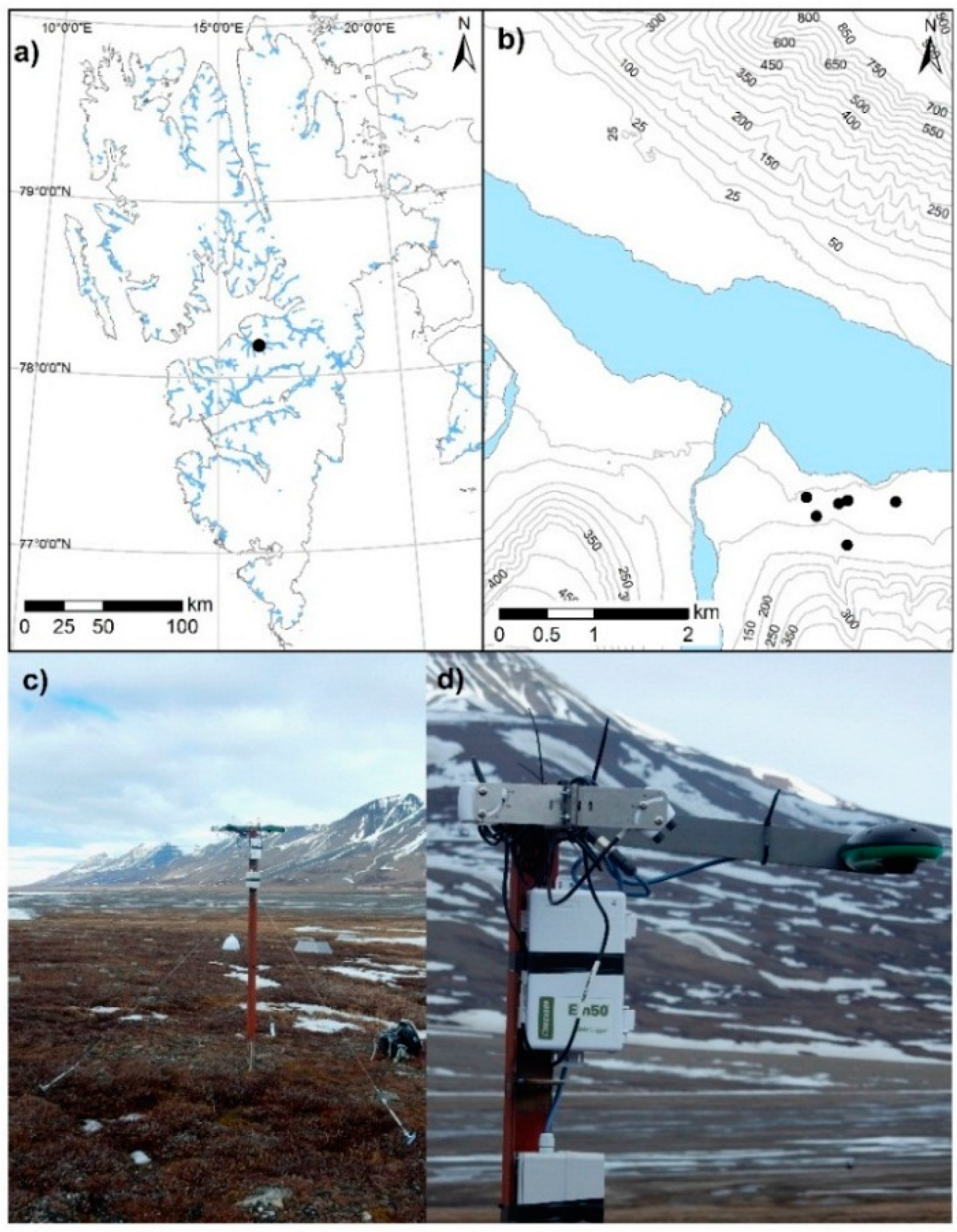
2.1. Study Area and Equipment Set-Up

The study was conducted in Adventdalen, central Svalbard, Norway (78°10′N, 16°02′E; Figure 1a,b). Adventdalen is one of the main valley systems in High Arctic Svalbard, with typically open tundra dominated by ridge, heath and marsh vegetation. The study area was situated on the valley floor between elevations of approximately 25–100 masl. Six locations were selected for sensor placement in order to record measures of plant greenness in different vegetation types. The vegetation types selected covered the dominating plant species of the area, such as: Cassiope tetragona; Dryas octopetala/Salix polaris; C. tetragona/D. octopetala. Likewise, graminoid/Salix polaris; graminoid/bryophyte and the Luzula spp. vegetation types were included. The ‘graminoid’ type contained a mixture of grasslike plant species, the majority of which were grasses. Our study was therefore representative of the vegetation found across lower elevations in Svalbard. These types cover up to 10.2% (for the Dryas and Cassiope communities), 3.4% (graminoid/Salix polaris), and 2.7% (graminoid/bryophytes) of the land cover based on the vegetation map for Svalbard [33]. Such High Arctic vegetation is characterised by having a very short growing season, low biomass productivity and plant heights of c. 5–10 cm [34]. At each location, sturdy metal support apparatus were driven into the soil substrate and secured with three metal guy ropes (Figure 1c). All sensors were securely attached to the support apparatus at a height of 2 m above ground level (Figure 1c,d). The design of the supporting apparatus minimised lateral movement due to wind and ensured measurements from the sensors were recorded consistently over the same fixed area throughout the season.

2.2. Sensor Descriptions and Monitoring Setup

Plant greenness was captured via two different near remote sensing techniques: NDVI, measured with sensors sensitive to red and near infra-red wavelengths; and greenness indices derived from images taken with standard digital red-green-blue wavelength (RGB) cameras. NDVI was recorded with two different devices; active and passive sensors. NDVI was measured at three of the fixed stations with in-situ Decagon Spectral Reflectance Sensors SRS-Nr [35] (hereafter Decagon sensor, which are now under test by several research teams, e.g., [36]) attached to programmable data loggers (Decagon Em50), which allowed full control of sensor activity. The Decagon sensors are passive sensor instruments and measure radiation in the near infrared (NIR: 810 ± 10 nm) and red (650 ± 10 nm) bandwidths. Each Decagon sensor was installed off-nadir (at 18°), thereby recording NDVI values over a spot diameter of 1.3 m. One upwards pointing Decagon hemispherical sensor SRS-Ni was installed and the incident radiation data collected was used to calibrate all the Decagon sensors. Data were recorded at four hourly intervals, beginning at midnight, for both NDVI and hemispherical reflectance sensor. Both NDVI and calibration values were taken as an average of six readings through the day. Sensors were installed on 4 June 2015 and retrieved on 31 August 2015, thereby resulting in data that covered 89 days of the growing season. NDVI was also measured directly at each plot with a Trimble Greenseeker Handheld Crop Sensor [37] (hereafter, Greenseeker). The Greenseeker is a portable, active sensor device that requires manual input for operation: a trigger is pulled which turns the sensor on, whereby light emitting diodes then beam near infrared (NIR: 780 ± 10 nm) and red (670 ± 10 nm) radiation onto the plant canopy, with the amount of light reflected back to the device then measured via silicon diodes. The device has no capacity for data logging, and it was not possible to take all measurements at the structured time intervals that coincided exactly with data recorded by the other sensors. However, since the Greenseeker is an active sensor that both emits and measures light, it is not limited by constraints such as cloud cover, atmospheric pollution, shadows and humidity that accompany passive systems [38] such as the Decagon sensors. Thus, although data from the Decagon sensors and Greenseeker device were recorded at different times of the day, NDVI values from the same location should be comparable. Operators were instructed to use the device for nadir sampling (thereby minimising any error associated with angle of view), at a height above ground level of 0.9 m (manufacturer instructions indicate use at 0.6–1.2 m) and thus measurements covered a spot diameter of 0.38 m. The Greenseeker was used to record NDVI values at each of the six monitoring locations at a minimum of twice weekly intervals between 18 June and 28 August 2015, giving 31, 33 or 34 days of data (dependent on location).

To enable greenness indices to be calculated for different plant species/groups throughout the growing season, images were captured with digital RGB cameras installed at each of the six monitoring locations. Five Brinno GardenWatch cameras [39] and a Cuddeback camera [40] were used. The GardenWatch camera has a resolution of 1.3 megapixels and recorded images every four hours, beginning at midnight from 6 June to 31 August, giving 87 days of data. The Cuddeback camera has a resolution of 20 megapixels and recorded one image every hour from 18 June to 31 August, giving 75 days of data. Each RGB camera was attached in the nadir position to the metal support apparatus described above (Figure 1d). The RGB cameras captured images over the same area that NDVI was recorded by Decagon sensors and the Greenseeker device and covered an area of 1.4 m × 1.1 m.

3. Data Preparation

Data from the Decagon sensors were calibrated using information on incident red and near infrared radiation collected by the hemispherical Decagon sensor. These data were used to calculate a calibration constant α:

$$\alpha =Ir/In$$

(1)

where Ir is the incident red radiation and In the incident near-infrared radiation. Calibration of the values recorded by the Decagon sensors was then possible using the formula:

$$\text{NDVI}=\frac{\alpha Rn-Rr}{\alpha Rn+Rr}$$

(2)

where Rn is the reflected near infrared radiation and Rr the reflected red radiation.

Vegetation indices (greenness indices) were calculated using information from the red, green and blue bands of the RGB images captured by the digital cameras throughout the growing season. Among six images taken every day, preferentially the mid-day images (time 12:00) were chosen. If fog, rain or other environmental conditions deteriorated image quality, the very best picture of that particular day was chosen. To ensure equivalent areas of vegetation at each location were compared throughout the growing season, masks were applied to specific defined areas of interest (AOI) in each of the images. Polygons were drawn around AOI, and converted to raster with the same extent and resolution as the images. From the areas within each mask, average digital numbers (DNs) were calculated for each vegetation type. For each RGB image, DN information was collected from the red, green and blue bands and was used to calculate three different greenness indices (2G_RBi [22], Channel G% [22,32] and Green-Red Vegetation Index (GRVI) [28,41]), as follows:

$$2\text{G}\_\text{RBi}=2G_{DN}-\left(R_{DN}+B_{DN}\right)$$

(3)

$$\text{Channel }G\%=G_{DN}/TotalRG{B}_{DN}$$

(4)

$$\text{GRVI}=\left(G_{DN}-R_{DN}\right)/\left(G_{DN}+R_{DN}\right)$$

(5)

where G_DN, R_DN and B_DN represent the digital numbers for the green, red and blue channels respectively.

4. Statistical Analyses

All statistical analyses were carried out in R (version 3.1.1). Firstly, to assess the ability of three different greenness indices (GRVI; 2G_RBi, and; channel G%) derived from RGB image data to capture the same patterns of change in plant greenness observed with NDVI values, we used Pearson’s correlations to compare values from those three greenness indices with NDVI values recorded by Decagon sensors and the Greenseeker device. Secondly, to determine how well the NDVI devices and the best RGB greenness index captured the changing patterns of plant greenness during the entire growing season, we used linear models with a second order polynomial function to determine the significance of relationships between day of year (DOY) and (i) Decagon-derived NDVI; (ii) Greenseeker-derived NDVI; and (iii) RGB greenness index. Typically, the NDVI values within a vegetation type or measuring NDVI of individual plant species, follows a unimodal or parabolic curve throughout a growing season [16]. The second order polynomial function is among the best-suited method to describe such pattern. Due to high day-to-day variability in GRVI values, these data were filtered. GRVI values outside the 95% confidence interval of the linear model have been omitted from the analyses to exclude obviously erroneous data. Finally, we used Pearson’s correlations to compare NDVI values recorded by Decagon sensors and the Greenseeker device in three different vegetation types (graminoid/S. polaris; C. tetragona; and C. tetragona/D. octopetala vegetation). Where significant correlations were evident, we then used linear models to determine the relationships between the NDVI values recorded by the two different sensors.

5. Results

5.1. Comparison of Different RGB Greenness Indices

We assessed the ability of three different greenness indices (GRVI, 2G_RBi and channel G%) derived from RGB images to record changes in plant greenness during the growing season by comparison with NDVI values obtained from the Decagon and Greenseeker devices. The GRVI had significant correlations with the NDVI values recorded in all vegetation types, with the exception of Luzula spp., where the sample size was small due to RGB equipment failure during the early part of the growing season (

Table 1. Pearson’s correlations between NDVI and three different RGB greenness indices in six different High Arctic vegetation types. The NDVI measurement instruments used were Decagon sensors (D) and a Greenseeker device (G). Greenness index values outside the 95% confidence interval of the linear model have been omitted from the analyses to exclude obviously erroneous data. t = t-statistic t_n = the valid sample numbers after filtering the time serial data. Statistically significant relationships are highlighted in bold.

Vegetation	NDVI Sensor	GRVI			2G_RBi			Channel G %
		t	p	r	t	p	r	t	p	r
Graminoid/Salix polaris	D	t82 = 16.55	<0.001	0.88	t80 = 9.11	<0.001	0.72	t81 = 9.76	<0.001	0.74
	G	t33 = 3.73	0.001	0.56	t30 = 2.62	0.014	0.44	t30 = 2.42	0.023	0.42
Cassiope tetragona	D	t76 = 11.45	<0.001	0.8	t78 = 14.52	<0.001	0.86	t75 = 12.34	<0.001	0.82
	G	t28 = 4.87	<0.001	0.69	t29 = 3.58	0.001	0.57	t27 = 3.01	0.006	0.52
Luzula spp.	G	t15 = 0.4	0.698	0.11	t15 = 3.01	0.01	0.64	t15 = 3.29	0.006	0.67
D. octopetala/S. polaris	G	t31 = 3.26	0.003	0.52	t29 = 3.01	0.006	0.5	t31 = 1.81	0.08	0.32
C. tetragona/D. octopetala	D	t81 = 13.76	<0.001	0.84	t79 = 12.05	<0.001	0.81	t80 = 10.54	<0.001	0.77
	G	t32 = 3.35	0.002	0.52	t32 = 1.0	0.325	0.18	t32 = 0.66	0.513	0.12
Graminoid/bryophyte	G	t30 = 6.87	<0.001	0.79	t30 = 9.44	<0.001	0.87	t30 = 6.59	<0.001	0.78

). The 2G_RBi and Channel G% indices similarly showed high significant correlations in all vegetation types, including Luzula spp., but not with the Greenseeker measurements in the mixed plot with Carex tetragona and Dryas octopetala (Table 1). Overall, GRVI showed the highest correlations of all three greenness indices.

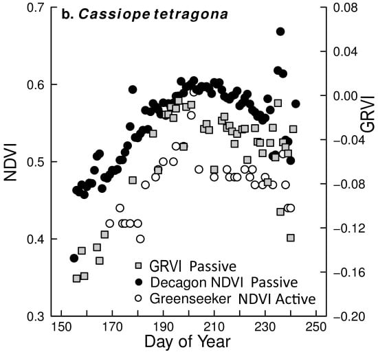
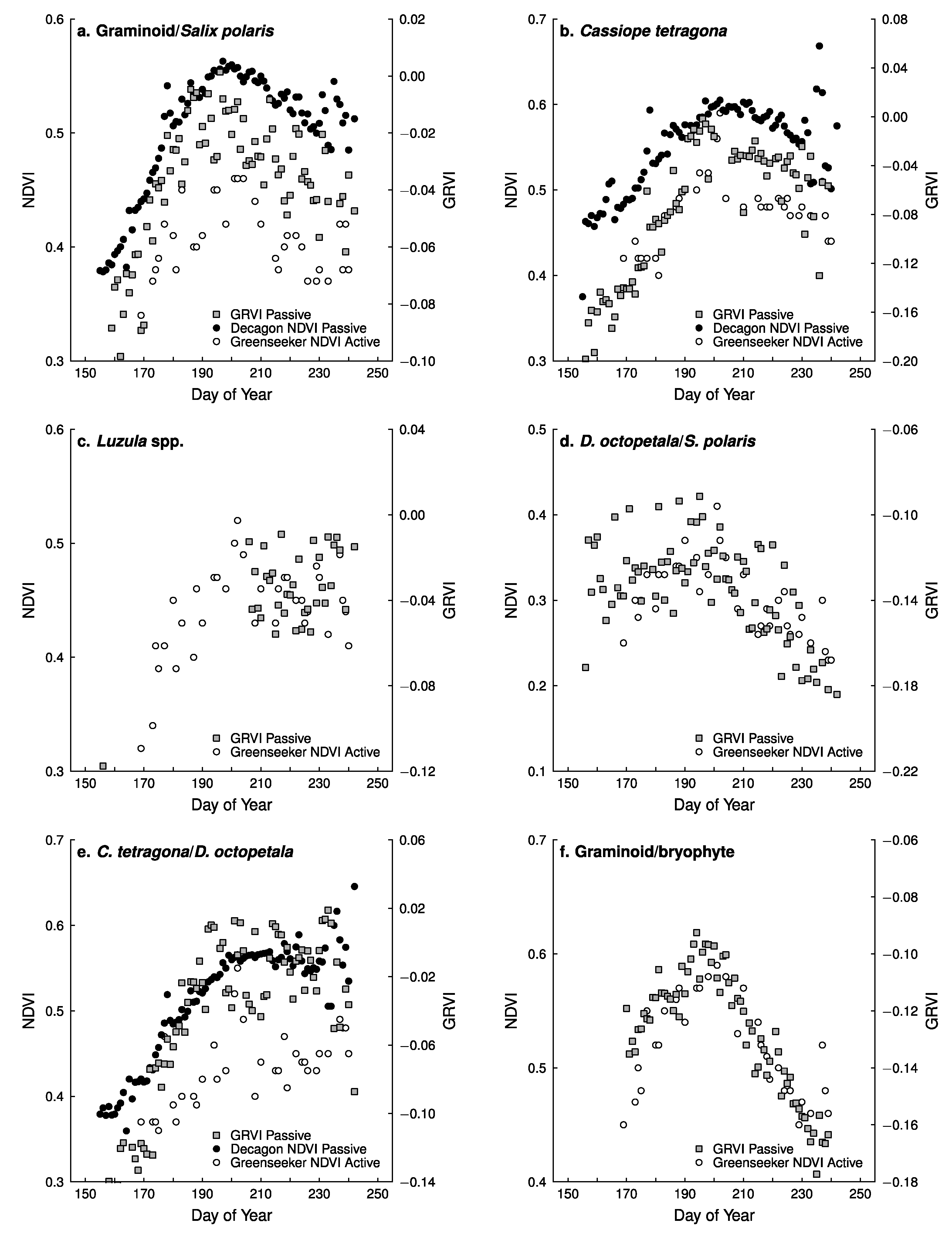
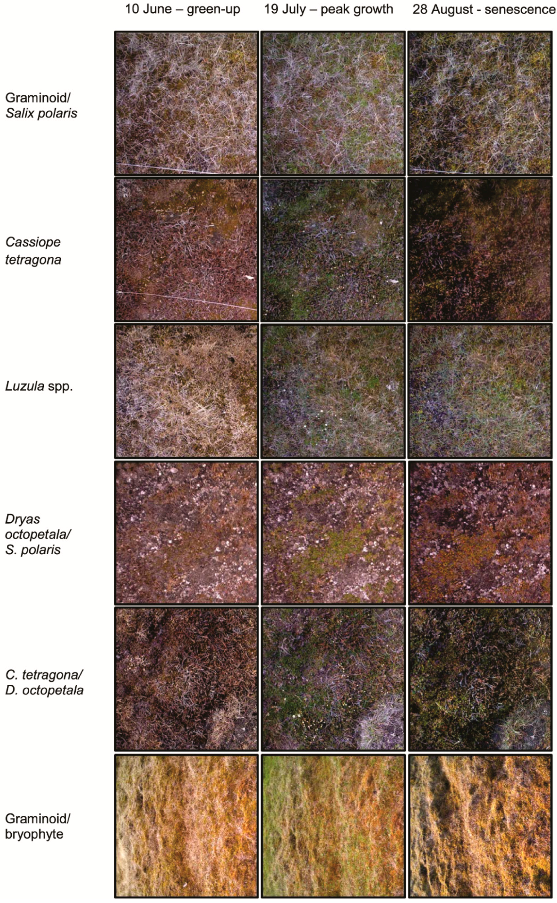
5.2. Capturing Changes in Plant Greenness during the Growing Season

The general pattern of change in plant greenness as the season progressed, recorded by NDVI sensors and the GRVI was similar in all vegetation types: values increased from the start of data recording, immediately after snow melted on 4 June (DOY 155), reached a maximum between 17 July (DOY 198) and 29 July (DOY 210), then after a period of peak growth the values decreased until the end of data recording on 30 August (DOY 242) when the first snowfall of autumn occurred (Figure 2). Hence, the start of the growing season (greening-up period) occurred from c. 4–19 June (DOY 155-170), the period of plant growth from c. 20 June–29 July (DOY 171-210) and senescence from c. 30 July (DOY 211) onwards (Figure 3). The evergreen shrub C. tetragona, however, seemed to have a slightly earlier start of the growing season, around 3 June (DOY 153-155), followed by the other species/species groups. The pattern during mid-season differed between some plant species/groups: e.g., where graminoids (mostly grasses) were present, both NDVI and GRVI values reached a sharp peak mid-season (DOY 195-200) and then dropped off fairly rapidly (Figure 2a,f). By contrast, the other plant species/groups (including Luzula) appeared to have a more prolonged period during mid-season when higher NDVI and GRVI values were maintained (Figure 2b–e). Towards the end of the season (from 18 August or DOY 230 onwards), relatively large daily variations in NDVI and GRVI values were evident in graminoid/S. polaris (Figure 2a); C. tetragona (Figure 2b); and C. tetragona/D. octopetala (Figure 2e) vegetation. In fact, at the end of August, on some occasions greenness index values equalled or exceeded values recorded during peak season, with this pattern most evident in the Decagon measurements, but also observed in the GRVI. The relationships between DOY and the plant greenness measure (NDVI or GRVI) were significant for all vegetation types, with the exception of GRVI values for the Luzula spp. (

Table 2. Relationships between day of year and values of different vegetation indices in six different High Arctic vegetation types. GRVI values outside the 95% confidence interval of the linear model have been omitted from the analyses to exclude obviously erroneous data.

Vegetation	Decagon NDVI			Greenseeker NDVI			GRVI
	F	p	R2	F	p	R2	F	p	R2
Graminoid/Salix polaris	F2,89 = 46.3	<0.001	0.52	F2,33 = 8.34	<0.001	0.36	F2,82 = 113.53	<0.001	0.74
Cassiope tetragona	F2,89 = 33.57	<0.001	0.44	F2,33 = 17.73	<0.001	0.54	F2,76 = 198.13	<0.001	0.84
Luzula spp.	-	-	-	F2,34 = 21.51	<0.001	0.58	F2,35 = 14.55	0.009	0.48
D. octopetala/S. polaris	-	-	-	F2,34 = 20.4	<0.001	0.57	F2,79 = 45.86	<0.001	0.55
C. tetragona/D. octopetala	F2,88 = 72.7	<0.001	0.63	F2,34 = 9.14	0.062	0.37	F2,81 = 214.37	<0.001	0.85
Graminoid/bryophyte	-	-	-	F2,31 = 22.32	<0.001	0.61	F2,69 = 204.36	<0.001	0.86

) where the sample size was small due to RGB equipment failure early in the season.

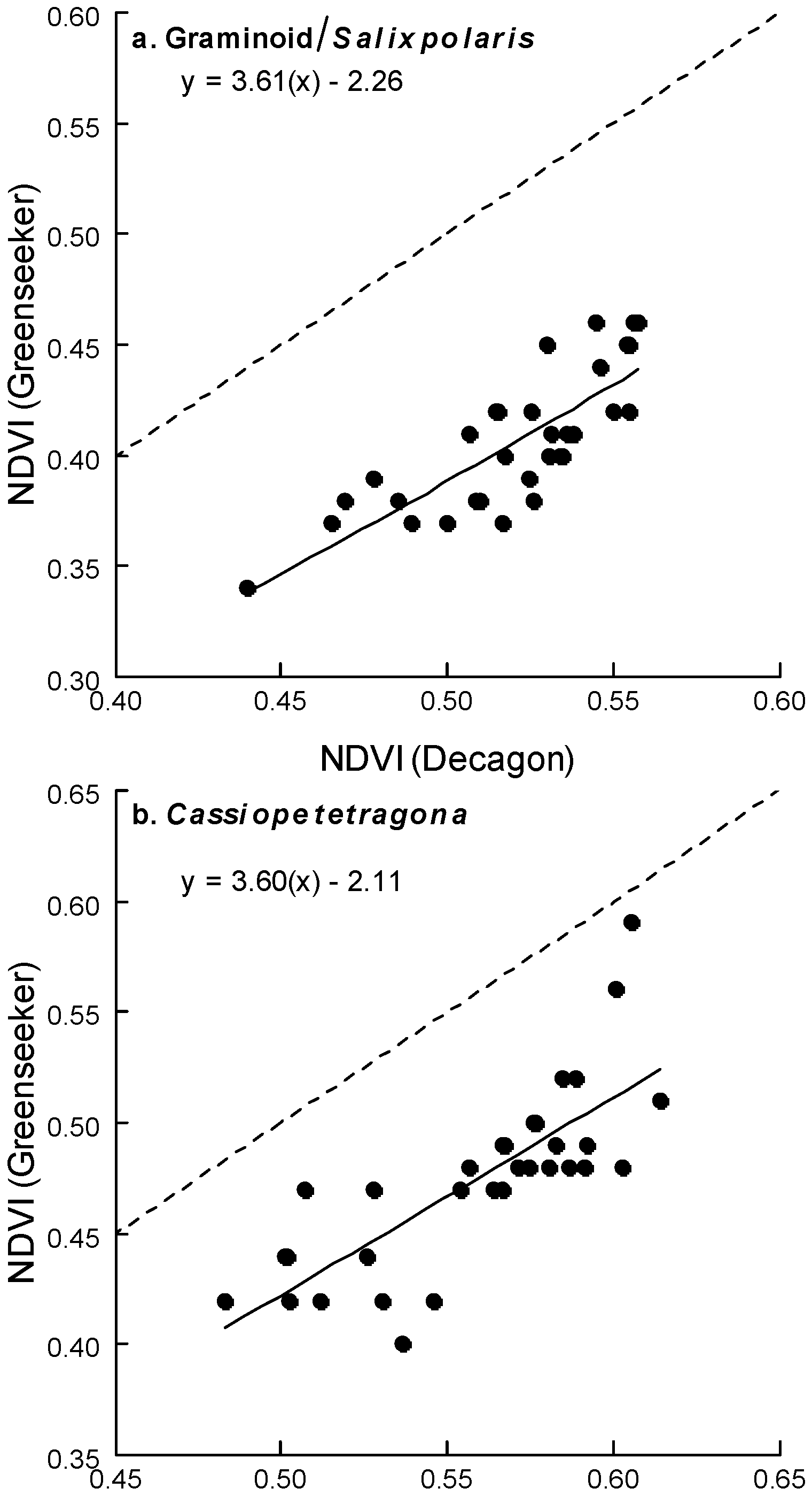
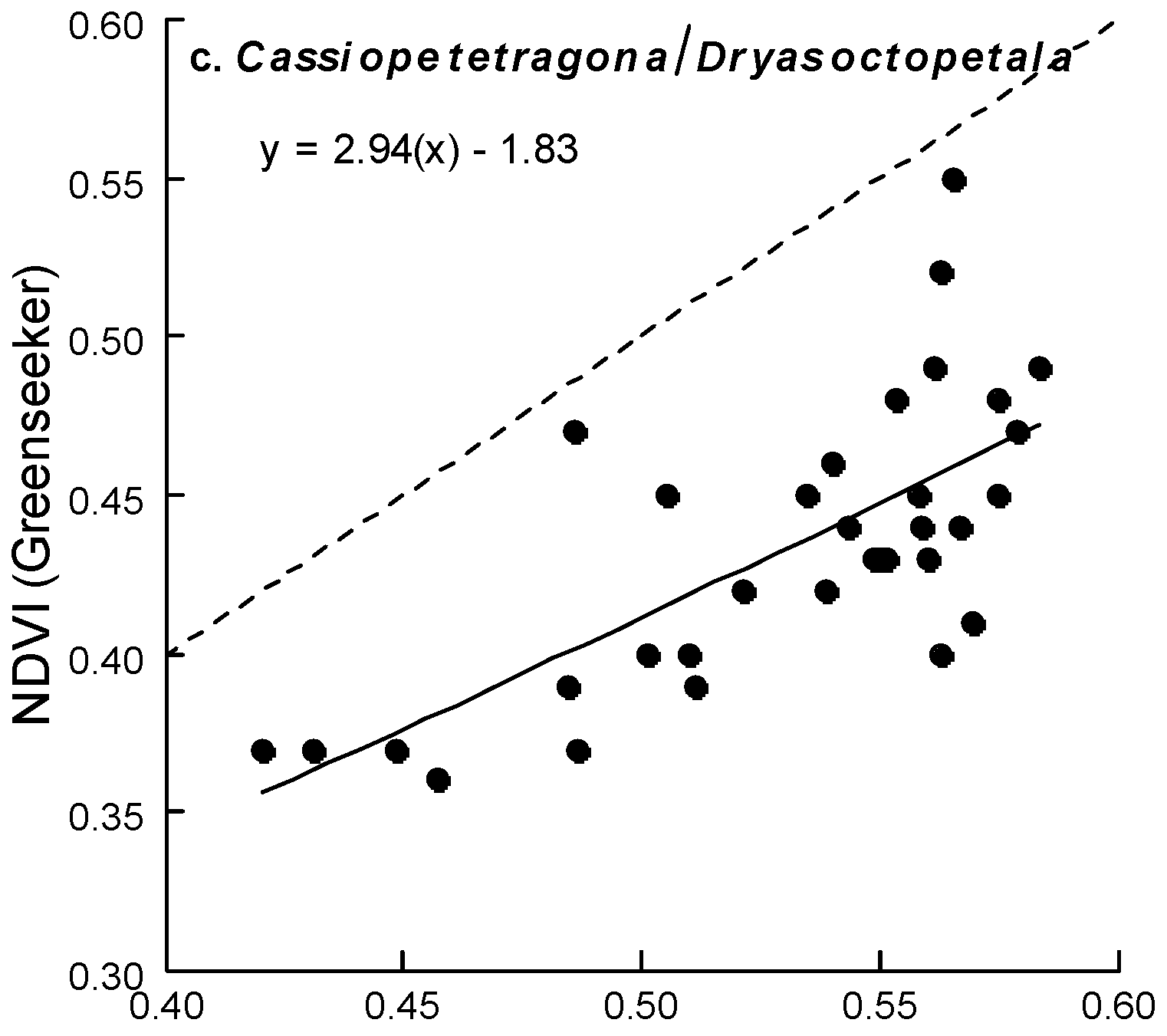
5.3. Comparison of Different NDVI Sensors

NDVI values recorded by the Decagon sensors and the Greenseeker device were well correlated in graminoid/S. polaris (t₃₁ = 7.47, p < 0.001, r = 0.80), C. tetragona (t₃₁ = 6.88, p < 0.001, r = 0.78) and C. tetragona/D. octopetala vegetation (t₃₂ = 5.55, p < 0.001, r = 0.70). Highly significant (p < 0.001) positive trends were evident in the relationships between NDVI recorded by the Decagon sensors and the Greenseeker device, in graminoid/S. polaris (Figure 4a), C. tetragona (Figure 4b) and C. tetragona/D. octopetala vegetation (Figure 4c). Looking across the entire growing season, it was evident that both NDVI devices (Decagon and Greenseeker) captured the changes in plant greenness throughout the growing season (Figure 2). However, NDVI values recorded by the Greenseeker device were consistently lower than those from the Decagon sensors (Figure 2a,b,e and Figure 4). Although the relationships between NDVI recorded by Decagon sensors and the Greenseeker device were very similar for graminoid/S. polaris (Figure 4a) and C. tetragona vegetation (Figure 4b), it did differ rather more for C. tetragona/D. octopetala vegetation (Figure 4c).

6. Discussion

There are many opportunities for using near remote sensing to capture environmental change in the remote Arctic. Indeed, digital cameras have been used to monitor such dynamic processes as snow cover and melt [42,43,44], glacier flow [45] and animal movements [46]. Here, we demonstrate the ability of inexpensive digital cameras and field-based NDVI devices to monitor the vegetation dynamics of six common and widespread plant species/groups in the High Arctic. Digital cameras captured data of sufficient quality throughout the growing season to enable the calculation of vegetation indices for each plant species/group. Of the three passive RGB derived greenness indices assessed, all were highly correlated with NDVI values in the plant groups studied, while GRVI showed the highest correlations. Thus, digital cameras can be successfully used for plant phenological monitoring at high latitudes.

Similar to our results, other studies that have compared the RGB derived vegetation indices GRVI, 2G_RBi, and Channel G% with NDVI found strong correlations [29,32], or similarity in the seasonal patterns observed [22,47]. Still, comparable results were not necessarily expected, since these studies were performed in different types of vegetation and described the phenology of broadleaf forest canopies, low-latitude grasslands and agricultural crops [22,29,32,47]. Indeed, even the heath, fen and copse vegetation monitored by Westergaard-Nielsen et al. [32] in Greenland with digital cameras, where they found channel G% and 2G_RBi indices to be significantly correlated with NDVI, was situated in the Low Arctic, where the vegetation structure and species composition is quite different to that found at higher latitudes. Although a study from Northern Svalbard (79°40′N) using imagery from the WorldView-2 satellite and an airborne RGB camera found channel G% values to be reasonably well correlated with NDVI, the vegetation surveyed (creeping saltmarsh grass (Puccinellia phryganodes) and moss-crust tundra communities) [48] was very different to that presented in this study. Our results therefore are of high relevance to further studies of the high-Arctic vegetation types presented in this paper. Furthermore, we found strong differences in the diurnal variation of the vegetation indices, which for 2G_RBi and Channel G% may be due to the inclusion of the blue channel, which is strongly affected by changes in solar irradiance such as cloudy conditions [49]. Cloud cover is common on Svalbard [50], therefore noise in the blue channel related to atmospheric conditions during our season-long study may explain the somewhat lower correlations for 2G_RBi and Channel G% compared to GRVI (Table 1). These diurnal variations were not apparent in the derivation of Channel G% values for vegetation in Northern Svalbard as that study used data from only one day [48]. Surprisingly, the spatial scale of operation did not appear to lead to different results, despite the fact that the cameras used in our study monitored vegetation over an area of c. 1 m², whereas previous studies monitored vegetation over the scale of a few tens to several hundreds of square meters.

We found the best result with the RGB derived GRVI (passive), which was significantly and strongly correlated with NDVI values despite fluctuations in the RGB camera derived index. Such variations may be due to diurnal differences in illumination, since the white balance and exposure settings of the RGB cameras we used were fixed to automatic with no option available to change these settings. Therefore, if the equipment allows, we recommend changing the white balance from automatic to a fixed setting as this can stabilise diurnal fluctuations in the indices calculated [51]. Nevertheless, our results support the findings of Motohka et al. [28] and von Bueren et al. [52] who found that the GRVI could be used to successfully monitor phenological change in vegetation. We have, therefore, extended the applicability of use of the GRVI to detect phenological change from low-latitude deciduous broadleaf and coniferous forest, grassland and rice paddy vegetation to include High Arctic vegetation. Motohka et al. [28] used the transition from negative to positive GRVI values to detect phenological change as they found negative values to equate with soils and positive values with green vegetation. However, we were unable to replicate this with High Arctic vegetation. Most of the GRVI values calculated in our study were negative, a likely reflection of the sparse cover of High Arctic plants [34] and the presence of black cryptogamic crust, which is widespread in the High Arctic [53], in almost all of our monitoring plots. Thus, given these limitations, the use of an absolute threshold GRVI value to define transitions between phenological stages in High Arctic vegetation may only be possible via monitoring at the individual species level rather than across mixed plant assemblages. In addition, if the main reason that the GRVI index performed better was the lack of blue band, would the values be just as good with a simple vegetation difference? Studies examining a variety of plants and stress factors in agricultural landscapes have found simple ratio indices to be most strongly affected by plant stress as well as phenological development [54,55], and this might also be the case for natural plants in Arctic environments. Nevertheless, the GRVI index clearly tracked the changes in plant greenness throughout the season and, hence, can be used effectively to monitor phenological change of High Arctic vegetation. We therefore recommend that future studies, making use of an RGB derived greenness index to monitor vegetation phenological change, assess more than one index in order to find the most representative for the plant species being studied.

As the growing season progressed, both NDVI measures (active and passive) and the passive RGB derived GRVI tracked similar patterns of changes in growth for all plant species monitored: values increased after snowmelt, reached a peak at mid-season before declining. However, as reported from field observational studies [11,56,57], there were noticeable differences in these patterns between species/groups. For instance, vegetation plots containing graminoids reached a well-defined and short peak in index values before declining sharply, whereas plots containing C. tetragona and D. octopetala had broader mid-season peak values as well as increased values at the end of the growing season/study period. For C. tetragona and D. octopetala this pattern may have been be due to recovery after set-back or injury to these species caused by harsh winter conditions. Indeed, large patches of dead C. tetragona vegetation were observed across Svalbard that summer (pers. obs.), presumably due to frost damage caused by lack of sufficient winter snow cover [58], possibly due to periods of snow thaw followed by re-freeze in the winter [59]. This species appears particularly susceptible to frost damage as the flower and leaf buds are erect, hence occurring at a greater height above ground (5–15 cm) than other High Arctic plant species that are characterised by having a prostrate structure [59]. The second peak in greenness values observed late in the season could also be partly attributed to the elongated growing season exhibited by bryophytes that lack senescence, as has been observed in Greenland [60]. This factor, however, depends on the amount of bryophytes present (in the study plot) that may take advantage of increased precipitation during the end of growing season in 2015, and this increased wetness may also contribute to sustained growth for stands of evergreen Cassiope tetragona that not had entered senescence. However, data from the graminoid/bryophyte community (Figure 2f), in which the bryophytes contributed significantly more to the signal than the other communities in this analysis, showed a rapid decrease from mid-season (DOY 200) towards the end of the season, indicating that the bryophyte activity may not explain the end season peak in the dwarf shrub (C. tetragona and D. octopetala) dominated plots. A late season peak is also shown in Graminoid/Salix polaris vegetation plot (Figure 2a). Both graminoids and Salix are deciduous, normally changing colour and losing leaves around DOY 230 [11] so extended late-season growth for these plants may be an unlikely explaination for the second peak observed in Figure 2a.

The second peak (DOY 225-240) is very marked in the Decagon NDVI data and to a lesser degree in the GRVI data, but not in the Greenseeker NDVI data. Other measurements by our research group recorded an increase in soil moisture in this same period. Whether our data really shows late season growth or, rather, differential instrumental response to increased moisture in late season, is impossible to determine with our present data set but is indeed an area for further research.

The increased variation in vegetation index values observed towards the end of the season was likely due to senescence producing changes in leaf colouration, a process that occurs over a more prolonged period than green-up, and also has species-specific timing [11,57,61]. Although Richardson et al. [22] found that RGB derived indices increased more slowly than NDVI values, we did not find this to be the case with High Arctic vegetation, thus suggesting that both NDVI and the GRVI used in this study captured the same vegetation attributes.

The greater variability in NDVI values obtained by the Greenseeker device compared with the Decagon sensors may be due to the Decagon sensors recording information at fixed times (midday), whereas the times at which the Greenseeker device recorded data were variable (but occurred between the hours of 10:00 and 14:00). However, the variability in values was low and in a study of pine forest in Finland, Wang et al. [62] found little daily variation in ground-based NDVI, particularly in the two hours either side of midday. Daily variations in NDVI may also have been caused by differences in weather conditions (sunny, partly cloudy and full cloud cover) as dense clouds are known to alter the quality of incident and reflected radiation [62]. Svalbard, however, has an oceanic climate with much cloud cover and few days with clear skies [50,63]. Consequently, during the growing season most days experienced cloud cover and we found little variation in NDVI values that could be attributed to weather conditions. Additionally, some differences in absolute NDVI values may be expected between the two sensor types because they operate at slightly different bandwidths [64]. However, the consistently lower values obtained from the active Greenseeker sensor compared to the passive Decagon sensors, also reported by Fitzgerald [65] and Yao et al. [66], can most likely be attributed to the different modes of operation that the two sensor types employ: the Greenseeker device is an active sensor, generating its own radiation for NDVI measurements, whereas the Decagon sensors are passive instruments, using reflected and incident radiation which has been calibrated to a constant using a hemispherical sensor [36]. For active sensors such as the Greenseeker, the advantage of not requiring calibration is nonetheless counterbalanced by the restricted bandwidth of radiation available for use as a light source. This limits their use to proximal sensing only [66] and reduces their performance when compared with that of passive sensors such as the Decagon devices [65]. However, as stated by Fitzgerald [65] and noted in this study, such differences in performance between active and passive sensors in measuring greenness are small. Therefore, as the efforts to inter-calibrate NDVI values derived from different satellite-based sensors show [67], it is evident that the same function could be performed with near remote sensing NDVI sensors, although not with the same accuracies as for the satellite-based sensors. A study by Yao et al. [66] comparing ASD Field Spec Pro spectrometer, CropScan MSR 16 and GreenSeeker RT 100 indicated that the vegetation indices from different sensors could be inter-calibrated. Their inter-calibration model showed that nearly equivalent NDVIs between these sensors could be achieved. Although there appears to be an absence of a universal equation representative of all High Arctic plant species that could be used to convert values obtained from different NDVI devices, species-specific inter-calibrations would certainly be possible. Combining the use of both types of devices could be helpful for extending the monitoring of phenological change in different plant species, thus enable spatial upscaling towards landscape level and above.

7. Conclusions

The near remote sensing devices Decagon and RGB digital camera (both passive) and Greenseeker (active), seem to offer great opportunities for monitoring phenological change in High Arctic vegetation:

• Comparing the Decagon and Greenseeker NDVI correlation for the three vegetation types equipped with Decagon sensors, the r was 0.80, 0.78 and 0.70 respectively.
• However, the (passive) Decagon sensor had higher correlations with GRVI than the (active) Greenseeker (Decagon 0.88, 0.8 and 0.84, Greenseeker 0.56, 0.69 and 0.52).
• Among the three RGB greenness indices derived from the digital cameras, the GRVI had the highest and most significant correlation of NDVI with both (passive) Decagon and (active) Greenseeker derived NDVI. Still, correlations of 2G_RBi and Channel G% with the Decagon were high in all vegetation types (ranging from 0.72 to 0.86), but less so with the Greenseeker where one (2G_RBi) or two (Channel G%) correlations were insignificant.
• The greater variability in NDVI measurement and poorer performance of (active) Greenseeker compared to (passive) Decagon indicate the need for more precise and rigid procedures for field measurement; the Greenseeker should be placed in a fixed position, aspect, slope and elevation for each field point measured.
• Correlations between NDVI values derived from (passive) Decagon/(active) Greenseeker and the RGB derived vegetation indices obtained from the digital cameras, especially the GRVI, indicate that both approaches capture similar vegetation attributes and are capable of being used to monitor phenological change in different plant species/groups. Thus, both NDVI sensors and RGB cameras could be used to establish an High Arctic near remote sensing monitoring network with the aim of validating high spatial resolution satellite based products.
• Inexpensive RGB cameras offer a more affordable alternative to the more specialized and expensive NDVI sensors for monitoring plant greenness. This may enable a greater spatial coverage for field campaigns.

References

1. Morisette, J.T.; Richardson, A.D.; Knapp, A.K.; Fisher, J.I.; Graham, E.A.; Abatzoglou, J.; Wilson, B.E.; Breshears, D.D.; Henebry, G.M.; Hanes, J.M.; et al. Tracking the rhythm of the seasons in the face of global change: Phenological research in the 21st century. Front. Ecol. Environ. 2009, 7, 253–260. [Google Scholar] [CrossRef]
2. Sparks, T.H.; Carey, P.D. The responses of species to climate over 2 centuries—An analysis of the Marsham phenological record, 1736–1947. J. Ecol. 1995, 83, 321–329. [Google Scholar] [CrossRef]
3. Root, T.L.; Price, J.T.; Hall, K.R.; Schneider, S.H.; Rosenzweig, C.; Pounds, J.A. Fingerprints of global warming on wild animals and plants. Nature 2003, 421, 57–60. [Google Scholar] [CrossRef] [PubMed]
4. Parmesan, C.; Yohe, G. A globally coherent fingerprint of climate change impacts across natural systems. Nature 2003, 421, 37–42. [Google Scholar] [CrossRef] [PubMed]
5. Menzel, A.; Sparks, T.H.; Estrella, N.; Koch, E.; Aasa, A.; Ahas, R.; Alm-Kubler, K.; Bissolli, P.; Braslavska, O.; Briede, A.; et al. European phenological response to climate change matches the warming pattern. Glob. Chang. Biol. 2006, 12, 1969–1976. [Google Scholar] [CrossRef]
6. Callaghan, T.V.; Tweedie, C.E.; Akerman, J.; Andrews, C.; Bergstedt, J.; Butler, M.G.; Christensen, T.R.; Cooley, D.; Dahlberg, U.; Danby, R.K.; et al. Multi-decadal changes in tundra environments and ecosystems: Synthesis of the international polar year-back to the future project (IPY-BTF). Ambio 2011, 40, 705–716. [Google Scholar] [CrossRef] [PubMed]
7. Kaufman, D.S.; Schneider, D.P.; McKay, N.P.; Ammann, C.M.; Bradley, R.S.; Briffa, K.R.; Miller, G.H.; Otto-Bliesner, B.L.; Overpeck, J.T.; Vinther, B.M.; et al. Recent warming reverses long-term arctic cooling. Science 2009, 325, 1236–1239. [Google Scholar] [CrossRef] [PubMed]
8. Brock, C.A.; Cozic, J.; Bahreini, R.; Froyd, K.D.; Middlebrook, A.M.; McComiskey, A.; Brioude, J.; Cooper, O.R.; Stohl, A.; Aikin, K.C.; et al. Characteristics, sources, and transport of aerosols measured in spring 2008 during the aerosol, radiation, and cloud processes affecting arctic climate (ARCPAC) project. Atmos. Chem. Phys. 2011, 11, 2423–2453. [Google Scholar] [CrossRef] [Green Version]
9. Vettoretti, G.; D’Orgeville, M.; Peltier, W.R.; Stastna, M. Polar climate instability and climate teleconnections from the arctic to the midlatitudes and tropics. J. Clim. 2009, 22, 3513–3539. [Google Scholar] [CrossRef]
10. Bjorkman, A.D.; Elmendorf, S.C.; Beamish, A.L.; Velland, M.; Henry, G.H.R. Contrasting effects of warming and increased snowfall on Arctic tundra plant phenology over the past two decades. Glob. Chang. Biol. 2015, 21, 4651–4661. [Google Scholar] [CrossRef] [PubMed]
11. Semenchuk, P.R.; Gillespie, M.A.K.; Rumpf, S.B.; Baggesen, N.S.; Elberling, B.; Cooper, E.J. High Arctic plant phenology is determined by snowmelt patterns but duration of phenological periods is fixed: An example of periodicity. Environ. Res. Lett. 2016, in press. [Google Scholar]
12. Oberbauer, S.F.; Elmendorf, S.C.; Troxler, T.G.; Hollister, R.D.; Rocha, A.V.; Bret-Harte, M.S.; Dawes, M.A.; Fosaa, A.M.; Henry, G.H.R.; Hoye, T.T.; et al. Phenological response of tundra plants to background climate variation tested using the international tundra experiment. Philos. Trans. R. Soc. B Biol. Sci. 2013, 368, 13–20. [Google Scholar] [CrossRef] [PubMed]
13. Prevéy, J.; Vellend, M.; Ruger, N.; Hollister, R.; Bjorkman, A.; Meyers-Smith, I.; Elmendorf, S.; Clark, K.; Cooper, E.J.; Elberling, B.; et al. Greater temperature sensitivity of plant phenology at colder sites: Implications for convergence across northern latitudes. Glob. Chang. Biol. 2016. submitted. [Google Scholar]
14. Kerr, J.T.; Ostrovsky, M. From space to species: Ecological applications for remote sensing. Trends Ecol. Evol. 2003, 18, 299–305. [Google Scholar] [CrossRef]
15. Turner, W.; Spector, S.; Gardiner, N.; Fladeland, M.; Sterling, E.; Steininger, M. Remote sensing for biodiversity science and conservation. Trends Ecol. Evol. 2003, 18, 306–314. [Google Scholar] [CrossRef]
16. Pettorelli, N.; Vik, J.O.; Mysterud, A.; Gaillard, J.M.; Tucker, C.J.; Stenseth, N.C. Using the satellite-derived NDVI to assess ecological responses to environmental change. Trends Ecol. Evol. 2005, 20, 503–510. [Google Scholar] [CrossRef] [PubMed]
17. Myneni, R.B.; Hall, F.G.; Sellers, P.J.; Marshak, A.L. The interpretation of spectral vegetation indexes. IEEE Trans. Geosci. Remote Sens. 1995, 33, 481–486. [Google Scholar] [CrossRef]
18. Tucker, C.J. Red and photographic infrared linear combinations for monitoring vegetation. Remote Sens. Environ. 1979, 8, 127–150. [Google Scholar] [CrossRef]
19. Stow, D.A.; Hope, A.; McGuire, D.; Verbyla, D.; Gamon, J.; Huemmrich, F.; Houston, S.; Racine, C.; Sturm, M.; Tape, K.; et al. Remote sensing of vegetation and land-cover change in arctic tundra ecosystems. Remote Sens. Environ. 2004, 89, 281–308. [Google Scholar] [CrossRef]
20. Pettorelli, N.; Pettorelli, N. Normalized Difference Vegetation Index; Oxford University Press: New York, NY, USA, 2013. [Google Scholar]
21. Bannari, A.; Morin, D.; Bonn, F.; Huete, A.R. A review of vegetation indices. Remote Sens. Rev. 1995, 13, 95–120. [Google Scholar] [CrossRef]
22. Richardson, A.D.; Jenkins, J.P.; Braswell, B.H.; Hollinger, D.Y.; Ollinger, S.V.; Smith, M.L. Use of digital webcam images to track spring green-up in a deciduous broadleaf forest. Oecologia 2007, 152, 323–334. [Google Scholar] [CrossRef] [PubMed]
23. Ide, R.; Oguma, H. Use of digital cameras for phenological observations. Ecol. Inform. 2010, 5, 339–347. [Google Scholar] [CrossRef]
24. Eastman, R.; Warren, S.G. Arctic cloud changes from surface and satellite observations. J. Clim. 2010, 23, 4233–4242. [Google Scholar] [CrossRef]
25. Hope, A.S.; Stow, D.A. Shortwave reflectance properties of arctic tundra landscapes. In Landscape Function and Disturbance in Arctic Tundra; Reynolds, J.F., Tenhunen, J.D., Eds.; Springer: Berlin/Heidelberg, Germany, 1996; pp. 155–164. [Google Scholar]
26. Beck, P.S.A.; Atzberger, C.; Høgda, K.A.; Johansen, B.; Skidmore, A.K. Improved monitoring of vegetation dynamics at very high latitudes: A new method using MODIS NDVI. Remote Sens. Environ. 2006, 100, 321–334. [Google Scholar] [CrossRef]
27. Toomey, M.; Friedl, M.A.; Frolking, S.; Hufkens, K.; Klosterman, S.; Sonnentag, O.; Baldocchi, D.D.; Bernacchi, C.J.; Biraud, S.C.; Bohrer, G.; et al. Greenness indices from digital cameras predict the timing and seasonal dynamics of canopy-scale photosynthesis. Ecol. Appl. 2015, 25, 99–115. [Google Scholar] [CrossRef] [PubMed]
28. Motohka, T.; Nasahara, K.N.; Oguma, H.; Tsuchida, S. Applicability of green-red vegetation index for remote sensing of vegetation phenology. Remote Sens. 2010, 2, 2369–2387. [Google Scholar] [CrossRef]
29. Migliavacca, M.; Galvagno, M.; Cremonese, E.; Rossini, M.; Meroni, M.; Sonnentag, O.; Cogliati, S.; Manca, G.; Diotri, F.; Busetto, L.; et al. Using digital repeat photography and eddy covariance data to model grassland phenology and photosynthetic CO2 uptake. Agric. For. Meteorol. 2011, 151, 1325–1337. [Google Scholar] [CrossRef]
30. Sonnentag, O.; Hufkens, K.; Teshera-Sterne, C.; Young, A.M.; Friedl, M.; Braswell, B.H.; Milliman, T.; O’Keefe, J.; Richardson, A.D. Digital repeat photography for phenological research in forest ecosystems. Agric. For. Meteorol. 2012, 152, 159–177. [Google Scholar] [CrossRef]
31. Buus-Hinkler, J.; Hansen, B.U.; Tamstorf, M.P.; Pedersen, S.B. Snow-vegetation relations in a high arctic ecosystem: Inter-annual variability inferred from new monitoring and modeling concepts. Remote Sens. Environ. 2006, 105, 237–247. [Google Scholar] [CrossRef]
32. Westergaard-Nielsen, A.; Lund, M.; Hansen, B.U.; Tamstorf, M.P. Camera derived vegetation greenness index as proxy for gross primary production in a low arctic wetland area. ISPRS J. Photogramm. Remote Sens. 2013, 86, 89–99. [Google Scholar] [CrossRef]
33. Johansen, B.E.; Karlsen, S.R.; Tømmervik, H. Vegetation mapping of Svalbard utilising Landsat TM/ETM+ data. Polar Rec. 2012, 48, 47–63. [Google Scholar] [CrossRef]
34. Rønning, O.I. The Flora of Svalbard; Norwegian Polar Institute: Tromsø, Norway, 1996. [Google Scholar]
35. Spectral Reflectance Sensor (SRS). Available online: https://www.decagon.com/en/canopy/canopy-measurements/spectral-reflectance-sensor-srs/ (accessed on 3 March 2016).
36. Gamon, J.A.; Kovalchuck, O.; Wong, C.Y.S.; Harris, A.; Garrity, S.R. Monitoring seasonal and diurnal changes in photosynthetic pigments with automated PRI and NDVI sensors. Biogeosciences 2015, 12, 4149–4159. [Google Scholar] [CrossRef]
37. GreenSeeker Handheld Crop Sensor. Available online: http://www.trimble.com/Agriculture/gs-handheld.aspx (accessed on 3 March 2016).
38. Inman, D.; Khosla, R.; Reich, R.M.; Westfall, D.G. Active remote sensing and grain yield in irrigated maize. Precis. Agric. 2007, 8, 241–252. [Google Scholar] [CrossRef]
39. Brinno Timelapse Cameras. Available online: http://www.brinno.com/html/GWC-intro.html (accessed on 3 March 2016).
40. Cuddeback. Available online: http://cuddeback.com/index.aspx (accessed on 3 March 2016).
41. Gitelson, A.A.; Kaufman, Y.J.; Stark, R.; Rundquist, D. Novel algorithms for remote estimation of vegetation fraction. Remote Sens. Environ. 2002, 80, 76–87. [Google Scholar] [CrossRef]
42. Bernard, E.; Friedt, J.M.; Tolle, F.; Griselin, M.; Martin, G.; Laffly, D.; Marlin, C. Monitoring seasonal snow dynamics using ground based high resolution photography. ISPRS J. Photogramm. Remote Sens. 2013, 75, 92–100. [Google Scholar] [CrossRef] [Green Version]
43. Hinkler, J.; Orbaek, J.B.; Hansen, B.U. Detection of spatial, temporal, and spectral surface changes in the Ny-Ålesund area 79 degrees N, Svalbard, using a low cost multispectral camera in combination with spectroradiometer measurements. Phys. Chem. Earth 2003, 28, 1229–1239. [Google Scholar] [CrossRef]
44. Hinkler, J.; Pedersen, S.B.; Rasch, M.; Hansen, B.U. Automatic snow cover monitoring at high temporal and spatial resolution, using images taken by a standard digital camera. Int. J. Remote Sens. 2002, 23, 4669–4682. [Google Scholar] [CrossRef]
45. Eiken, T.; Sund, M. Photogrammetric methods applied to Svalbard glaciers: Accuracies and challenges. Polar Res. 2012, 31, 16–20. [Google Scholar] [CrossRef]
46. Tape, K.D.; Gustine, D.D. Capturing migration phenology of terrestrial wildlife using camera traps. Bioscience 2014, 64, 117–124. [Google Scholar] [CrossRef]
47. Inoue, T.; Nagai, S.; Kobayashi, H.; Koizumi, H. Utilization of ground-based digital photography for the evaluation of seasonal changes in the aboveground green biomass and foliage phenology in a grassland ecosystem. Ecol. Inform. 2015, 25, 1–9. [Google Scholar] [CrossRef]
48. Thuestad, A.E.; Tømmervik, H.; Solbø, S.A.; Barlindhaug, S.; Flyen, A.C.; Myrvoll, E.R.; Johansen, B. Monitoring cultural heritage environments in Svalbard: Smeerenburg, a whaling station on Amsterdam island. EARSeL eProc. 2015, 14, 37–50. [Google Scholar]
49. Richardson, A.D.; Braswell, B.H.; Hollinger, D.Y.; Jenkins, J.P.; Ollinger, S.V. Near-surface remote sensing of spatial and temporal variation in canopy phenology. Ecol. Appl. 2009, 19, 1417–1428. [Google Scholar] [CrossRef] [PubMed]
50. Van der Wal, R.; Stien, A. High-arctic plants like it hot: A long-term investigation of between-year variability in plant biomass. Ecology 2014, 95, 3414–3427. [Google Scholar] [CrossRef]
51. Mizunuma, T.; Wilkinson, M.; Eaton, E.L.; Mencuccini, M.; Morison, J.I.L.; Grace, J. The relationship between carbon dioxide uptake and canopy colour from two camera systems in a deciduous forest in Southern England. Funct. Ecol. 2013, 27, 196–207. [Google Scholar] [CrossRef]
52. Von Bueren, S.K.; Burkart, A.; Hueni, A.; Rascher, U.; Tuohy, M.P.; Yule, I.J. Deploying four optical UAV-based sensors over grassland: Challenges and limitations. Biogeosciences 2015, 12, 163–175. [Google Scholar] [CrossRef]
53. Pushkareva, E.; Pessi, I.S.; Wilmotte, A.; Elster, J. Cyanobacterial community composition in arctic soil crusts at different stages of development. FEMS Microbiol. Ecol. 2015, 91, 10–15. [Google Scholar] [CrossRef] [PubMed]
54. Carter, G.A. Ratios of leaf reflectances in narrow wavebands as indicators of plant stress. Int. J. Remote Sens. 1994, 15, 697–703. [Google Scholar] [CrossRef]
55. Lee, Y.J.; Yang, C.M.; Change, K.W.; Shen, Y. A simple spectral index using reflectance of 735 nm to assess nitrogen status of rice canopy. Agron. J. 2008, 100, 205–212. [Google Scholar] [CrossRef]
56. Rumpf, S.B.; Semenchuk, P.R.; Dullinger, S.; Cooper, E.J. Idiosyncratic responses of high arctic plants to changing snow regimes. PLoS ONE 2014, 9, 10–13. [Google Scholar] [CrossRef] [PubMed] [Green Version]
57. Cooper, E.J.; Dullinger, S.; Semenchuk, P. Late snowmelt delays plant development and results in lower reproductive success in the high arctic. Plant Sci. 2011, 180, 157–167. [Google Scholar] [CrossRef] [PubMed] [Green Version]
58. Callaghan, T.V.; Carlsson, B.A.; Tyler, N.J.C. Historical records of climate-related growth in Cassiope tetragona from the arctic. J. Ecol. 1989, 77, 823–837. [Google Scholar] [CrossRef]
59. Semenchuk, P.R.; Elberling, B.; Cooper, E.J. Snow cover and extreme winter warming events control flower abundance of some, but not all species in high arctic Svalbard. Ecol. Evol. 2013, 3, 2586–2599. [Google Scholar] [CrossRef] [PubMed] [Green Version]
60. Arndal, M.F.; Illeris, L.; Michelsen, A.; Albert, K.; Tamstorf, M.; Hansen, B.U. Seasonal variation in gross ecosystem production, plant biomass, and carbon and nitrogen pools in five high arctic vegetation types. Arct. Antarct. Alpine Res. 2009, 41, 164–173. [Google Scholar] [CrossRef]
61. Abbandonato, H.; Semenchuk, P.R.; Elberling, B.; Cooper, E.J. Snowmelt timing and soil temperature as important drivers for autumn senescence in High Arctic Svalbard. Environ. Res. Lett. 2016, in press. [Google Scholar]
62. Wang, Q.; Tenhunen, J.; Dinh, N.Q.; Reichstein, M.; Vesala, T.; Keronen, P. Similarities in ground- and satellite-based NDVI time series and their relationship to physiological activity of a scots pine forest in finland. Remote Sens. Environ. 2004, 93, 225–237. [Google Scholar] [CrossRef]
63. Van der Wal, R.; Hessen, D.O. Analogous aquatic and terrestrial food webs in the high arctic: The structuring force of a harsh climate. Perspect. Plant Ecol. Evol. Syst. 2009, 11, 231–240. [Google Scholar] [CrossRef]
64. Sakamoto, T.; Gitelson, A.A.; Nguy-Robertson, A.L.; Arkebauer, T.J.; Wardlow, B.D.; Suyker, A.E.; Verma, S.B.; Shibayama, M. An alternative method using digital cameras for continuous monitoring of crop status. Agric. For. Meteorol. 2012, 154, 113–126. [Google Scholar] [CrossRef]
65. Fitzgerald, G.J. Characterizing vegetation indices derived from active and passive sensors. Int. J. Remote Sens. 2010, 31, 4335–4348. [Google Scholar] [CrossRef]
66. Yao, X.F.; Yao, X.; Jia, W.Q.; Tian, Y.C.; Ni, J.; Cao, W.X.; Zhu, Y. Comparison and intercalibration of vegetation indices from different sensors for monitoring above-ground plant nitrogen uptake in winter wheat. Sensors 2013, 13, 3109–3130. [Google Scholar] [CrossRef] [PubMed]
67. Steven, M.D.; Malthus, T.J.; Baret, F.; Xu, H.; Chopping, M.J. Intercalibration of vegetation indices from different sensor systems. Remote Sens. Environ. 2003, 88, 412–422. [Google Scholar] [CrossRef]
Figure 1. Maps of (a) location of the study area in Svalbard; (b) sensor locations in Adventdalen, Central Svalbard; (c) and (d) images of the Decagon Normalized Difference Vegetation Index (NDVI) surface reflectance sensor, hemispherical sensor and red-green-blue wavelength (RGB) camera. The black symbol in (a) shows the location of the study site in Svalbard and in (b) the locations of the six monitoring sites in Adventdalen. Rivers are indicated in blue in (a,b) and contour lines with elevations (masl) are also displayed in (b).
Remotesensing 08 00847 g001
Figure 2. NDVI and greenness index values from six different High Arctic plant communities throughout the growing season. Readings were taken between 5 June (day of year = 156) and 30 August (day of year = 242) 2015 in: (a) Graminoid/Salix polaris; (b) Cassiope tetragona; (c) Luzula spp.; (d) Dryas octopetala/Salix polaris; (e) Cassiope tetragona/Dryas octopetala; and (f) Graminoid/bryophyte vegetation. NDVI was recorded using Decagon surface reflectance sensors (black circles) and a Trimble Greenseeker handheld sensor (open circles); the Green-Red Vegetation Index (GRVI) values (grey squares) were calculated from red and green channel data from RGB images.
Remotesensing 08 00847 g002
Figure 3. RGB camera images of six High Arctic plant species/groups from Svalbard during plant green-up (10 June DOY 161), peak plant growth (19 July DOY 200) and senescence (28 August DOY 240).
Remotesensing 08 00847 g003
Figure 4. Comparison of Decagon surface reflectance sensor-derived NDVI (passive) and Trimble Greenseeker-derived NDVI (active) from different vegetation types in High Arctic Svalbard. Readings were taken between 18 June (day of year = 169) and 28 August (day of year = 240) 2015 in: (a) Graminoid/Salix polaris; (b) Cassiope tetragona, and; (c) Cassiope tetragona/Dryas octopetala vegetation. Fitted lines from the linear models are shown. The closer points are to the dashed line (y = x), the more similar are the values recorded by the Decagon sensors and the Greenseeker device.
Remotesensing 08 00847 g004aRemotesensing 08 00847 g004b