Tropical Peatland Burn Depth and Combustion Heterogeneity Assessed Using UAV Photogrammetry and Airborne LiDAR

Abstract

We provide the first assessment of tropical peatland depth of burn (DoB) using structure from motion (SfM) photogrammetry, applied to imagery collected using a low-cost, low-altitude unmanned aerial vehicle (UAV) system operated over a 5.2 ha tropical peatland in Jambi Province on Sumatra, Indonesia. Tropical peat soils are the result of thousands of years of dead biomass accumulation, and when burned are globally significant net sources of carbon emissions. The El Niño year of 2015 saw huge areas of Indonesia affected by tropical peatland fires, more so than any year since 1997. However, the Depth of Burn (DoB) of these 2015 fires has not been assessed, and indeed has only previously been assessed in few tropical peatland burns in Kalimantan. Therefore, DoB remains arguably the largest uncertainty when undertaking fire emissions calculations in these tropical peatland environments. We apply a SfM photogrammetric methodology to map this DoB metric, and also investigate combustion heterogeneity using orthomosaic photography collected using the UAV system. We supplement this information with pre-burn airborne light detection and ranging (LiDAR) data, reducing uncertainty by estimating pre-burn soil height more accurately than from interpolation of adjacent unburned areas alone. Our pre-and post-fire Digital Terrain Models (DTMs) show accuracies of 0.04 and 0.05 m (root-mean-square error, RMSE) respectively, compared to ground-based global navigation satellite system (GNSS) surveys. Our final DoB map of a 5.2 ha degraded peat swamp forest area neighboring Berbak National Park (Sumatra, Indonesia) shows burn depths extending from close to zero to over 1 m, with a mean (±1σ) DoB of 0.23 ± 0.19 m. This lies well within the range found by the few other studies available (on Kalimantan; none are available on Sumatra). Our combustion heterogeneity analysis suggests the deepest burns, which extend to ~1.3 m, occur around tree roots. We use these DoB data within the Intergovernmental Panel on Climate Change (IPCC) default equation for fire emissions to estimate mean carbon emissions as 134 ± 29 t·C∙ha⁻¹ for this peatland fire, which is in an area that had not had a recorded fire previously. This is amongst the highest per unit area fuel consumption anywhere in the world for landscape fires. Our approach provides significant uncertainty reductions in such emissions calculations via the reduction in DoB uncertainty, and by using the UAV SfM approach this is accomplished at a fraction of the cost of airborne LiDAR—albeit over limited sized areas at present. Deploying this approach at locations across Indonesia, sampling a variety of fire-affected landscapes, would provide new and important DoB statistics for producing optimized carbon and greenhouse gas (GHG) emissions estimates from peatland fires.

1. Introduction

Fires in tropical peatlands are a well-recognised source of carbon emissions to the atmosphere [1,2], and in 2015 levels of landscape burning in Indonesia were greatly exacerbated by a drought brought on by the strong El Niño. Estimates suggest that over 0.8 × 10⁶ ha of Indonesian peatlands burned in September and October 2015, releasing 11.3 Tg of carbon to the atmosphere per day, equating to more CO₂ than the entire European Union emitted in the same period [3].

After most of the above-ground biomass has burned, peat fires continue smouldering, spreading deep into the peat layer and burning away the carbon-rich soil [4]. Fire propagation is via pyrolysis (absorption of heat and release of gas, producing char) and oxidation (organic matter/char is consumed producing ash and gases in the presence of oxygen). The majority of emissions occur through the oxidation of char, rather than the pyrolysis of peat [5]. Char oxidation is evident from the ash that remains post-fire (Figure 1), and also the presence of char beneath. Complete combustion (and so the greatest Depth of Burn, DoB) is suggested to occur mostly around the roots of trees [6], potentially because of reduced soil moisture [7,8,9].

To estimate carbon and greenhouse gas (GHG) emissions from tropical peatland fires requires quantification of the amount of peat consumed. This can be done by assessing the amount of thermal radiant energy emitted by the burning peat—sometimes coupled with atmospheric assessments of the emitted species [3]—but is most commonly done by measuring the burned area and multiplying this by the estimated depth of burn (DoB) and pre-fire peat bulk density [10,11]. Due to the high bulk density and carbon content of peat, and the fact that DoB can extend to tens of cm, landscape fire fuel consumption per unit area in tropical peatlands is amongst the highest of any biome worldwide. However, the range in DoBs expected between different types of peatland biome and between different fires means that the carbon emission estimates derived from the burned area based approach remain rather uncertain, and whilst burned area and peat bulk density are increasingly well measured [12,13,14], few DoB estimates exist currently. The existing spatially explicit DoB measurements available, beyond a few point-based measures derived via the use of metal rods to assess subsidence after burning [1,4], have mostly been assessed using light detection and ranging (LiDAR) approaches [9,15].

LiDAR can measure surface topography (to within a few cm) by timing the return of an emitted laser pulse, and airborne LiDAR enables difficult-to-access landscapes to be surveyed quickly and accurately [16]. However, the costs of LiDAR surveys are prohibitive. Furthermore, DoB is most accurately measured by differencing pre- and post-burn digital terrain models (DTMs), but collection of the former data requires predicting where (and to some extent when) landscape fires will occur. To date, only one study has estimated peatland depth of burn by differencing the pre- and post- burn peat DTMs of the same area of peat swamp forest (in the USA), and returned a mean DoB of 0.47 m (with a standard deviation in this mean of ±0.18 m) over a 25 km² burned area [16]. Other airborne LiDAR-based studies have not had pre-burn elevation data available, and so have either measured the mean elevation difference between a burned and adjacent unburned area [9], or have reconstructed a pre-burn surface model using interpolations from adjacent unburned topography [15]. While these two post-burn only approaches may not capture DoB as well as if pre-burn topographic data were available, they have provided unique assessments of peatland DoB over very large areas (3750 and 4000 ha respectively).

Most in situ peatland fire research has focused on temperate or boreal regions [6,17,18,19,20], but as tropical peat is derived from different vegetation types and contains a much higher fraction of woody material [21], more work is required to assess DoB in tropical peatlands. Work in [4] demonstrates the thermal and physical burn characteristics of tropical peat fires using experimental plots in Kalimantan (Indonesia), albeit at very small-scale (9 m² area) where point-based measurements can suffice. Unmanned aerial vehicles (UAVs) provide a flexible platform to cover much larger areas, and via photogrammetric analysis, the imagery captured by such platforms may also be suitable for mapping DoB. However, to our knowledge, this has yet to be attempted in any biome worldwide.

Using overlapping, high resolution aerial photographs taken from different viewing angles, Structure from Motion techniques (SfM) reconstruct point clouds (similar to those provided by LiDAR methods), which can then be used to produce digital terrain models (DTMs) and orthomosaic aerial images (orthophotos). The accuracy of DTMs from SfM techniques is affected by the amount of image overlap, camera calibration and sensor size, image quality [22], photogrammetry algorithm [23], UAV flying altitude [24,25], camera viewing angle [22,26,27], ground control point accuracy, and ground cover heterogeneity (i.e., featureless surfaces can cause additional error [22,26,28,29]). Fortunately, modern photogrammetric software can automatically detect tie points between photos, regardless of changes in camera orientation or survey distance, providing there is sufficient overlap between photos (50%–90%). DTM vertical accuracy and precision of UAV surveys is reportedly comparable to that of airborne LiDAR, with [28] achieving a mean 0.015 m bias (root-mean-squared deviation (RMSD) = 0.220 m) in a coastal setting by comparing UAV- and Terrestrial Laser Scanner (TLS)-derived DTMs, [30] achieving between 0.004 and 0.04 m accuracy and 0.02 and 0.07 m precision for a river area and [31] generating DTMs accurate to 0.025–0.04 m in a dune environment.

Here, we assess the applicability and accuracy of a low-cost UAV system for assessing peat fire DoB for the first time. Our focus is a previously unburned but degraded peat swamp forest, along with a previously burned shrub land, both located on Sumatra, Indonesia. Pre- and post-fire topography from LiDAR- and UAV-derived DTMs are compared to assess peat depth of burn (DoB) across the area, whilst the aerial photography is also used to assess combustion heterogeneity.

2. Materials and Methods

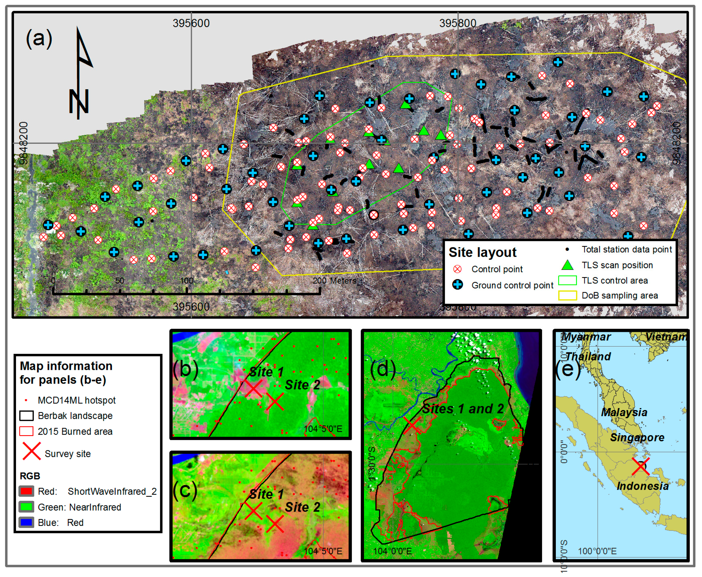
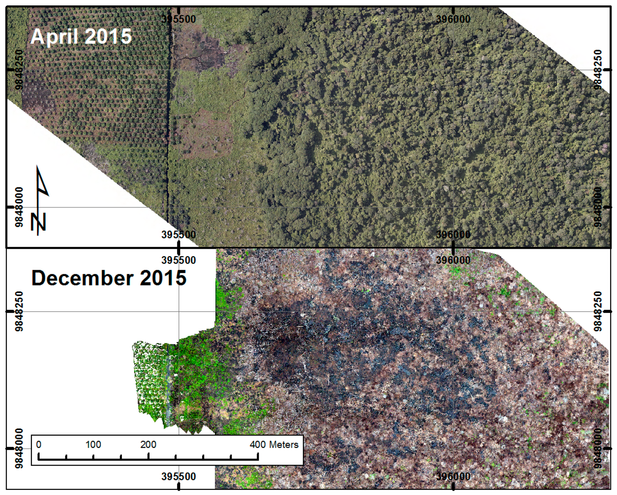
2.1. Sites

The two study sites (

Table 1. Summary information for two survey sites. Results from the surveys on Site 1 were used to develop the survey methods and objectives for Site 2. Vegetation height was estimated by measuring the height of standing trees in pre-burn light detection and ranging (LiDAR).

Site Number	Land Cover	Active Fire Detection Date	Pre-Fire Vegetation	Mean/Max Vegetation Height (m)	Area (ha)
1	Shrub	17–26 August 2015	Ferns, few short trees	2/20	58.4
2	Forest	4 October 2015	Degraded peat swamp forest	11/43	5.2

) are based within the area of interest of a Government of Indonesia-approved REDD+ (Reducing Emissions from Deforestation and forest Degradation) project [32]. Much of the area is degraded to some extent, with drainage canals and logging trails penetrating deep into the National Park [33]. The whole area is dominated by organosols (over 55% organic matter [34], ranging from 4.1 to 6.4 m deep, which equates to an estimated carbon density of between 2252 and 3228 t·C·ha⁻¹ [35]. Much of the landscape around Berbak National Park has been fire-affected (Figure 2b–d), with fires mostly associated with forest degradation and drainage of the peat for agriculture. Fires became especially widespread during the drought that accompanied the very strong 1997 El Niño [36]. Site 1 had burned previously (as evidenced by Moderate Resolution Imaging Spectroradiometer (MODIS) MCD14ML hotspot detections) but Site 2 had not. Sites 1 and 2 studied here were burned during the 2015 fires that accompanied the strong El Niño driven drought, and are situated within and near the boundaries of Taman Hutan Raya National Forest reserve (TAHURA), in Muaro Jambi district, Jambi Province, Sumatra, Indonesia (North West and South East limits of the area are 104.0481°W, 1.3650°S and 104.0656°W, 1.3750°S respectively; WGS84 datum, Figure 2).

Pre-fire 30 m spatial resolution imagery from Landsat 7 (ETM+) and Landsat 8 (OLI) was masked for cloud, smoke and shadow and used to stratify the landscapes into forest, shrub/regrowth forest, agriculture, water and burned area. Following [33,34], the stratification was based on maximum likelihood classification of tasselled cap-transformed optical data, because these different land covers are well differentiated by differences in brightness, greenness and wetness (e.g., forests tend to be dark, green and more moist compared to agricultural areas). Survey sites were selected using MODIS MCD14ML active fire detections [37] (Figure 2b,c)) based on their land cover strata and coincident location with the pre-burn LiDAR survey (Table 1), and are representative of land cover classes which typically burn in the Berbak Landscape.

Site 1 (shrub site) was surveyed between 20 August and 7 September 2015, fires on the site itself were extinguished. Site 2 (forest edge site) burned in October 2015 for approximately 15 days (Figure 3) and was surveyed between 8 and 16 December 2015 after all burning in the Berbak landscape had ceased.

2.2. Data Collection

2.2.1. Airborne LiDAR Survey

Before the fires of 2015, an airborne LiDAR survey was conducted on 21 April 2015 using an Orion M300 airborne LiDAR system (Teledyne Optech Inc., Vaughan, ON, Canada). Flying altitude was 850 m above ground level (agl) at a flight speed of 90 knots and the LiDAR operated with a laser pulse rate of 275 kHz (in multi-pulse mode), scan frequency of 45 Hz and scan ½ angle of 22 degrees, giving a point return density of 10 points per m², with up to four discrete returns available. Aerial RGB imagery was also acquired simultaneous with the LiDAR data at 0.1 m resolution (Figure 3). Both datasets were projected and delivered for use in the study with a UTM (Universal Transverse Mercator Coordinate System) 48S (WGS84 datum) and mean sea level (MSL) vertical datum.

2.2.2. UAV System

The UAV used was a small, very lightweight and low-cost quadcopter (a Dà-Jiāng Innovations Science and Technology Co., Ltd. (DJI), Shenzhen, China), Phantom 2; total mass ~1 kg and available at less than Great Britain Pound (GBP) 500). The UAV flight paths, speed, altitude and heading were calculated to ensure >70% forward and sidewards photo overlap, and waypoints were pre-programmed in DJI Groundstation for I-Pad software (DJI Innovations) and communicated to the UAV via a 2.4 GHz wireless datalink (

Table 2. Summary of the UAV surveys (Site 2). The flight altitude reported by the Dà-Jiāng Innovations Science and Technology Co., Ltd. (DJI) ground station and Flytrex Core 2 black box differed by the flight altitude calculated by Agisoft Photoscan where the average error was 3.96 m (root-mean-squared deviation (RMSD) = 4.99 m). The naming convention for the flight name is “planned flight altitude” “camera angle abbreviation” (e.g., 30 m_O is the name given to the flight planned to fly at 30 m, with an oblique camera angle; N = nadir camera angle).

Flight Name	Flight Altitude (m)	Total Images	Route Spacing (m)	Shooting Distance (m)	Horizontal Speed (m·s−1)
30 m_O	36	1173	8	5	5
30 m_N	34	1176	8	5	5
35 m_O	37	976	9	6	6
35 m_N	39	1358	9	6	6
40 m_O	44	1086	10.5	7	7
40 m_N	42	1125	10.5	7	7
50 m_N	50	959	13	9	9
60 m_O	70	814	16	10.5	10

). A Ricoh GR digital camera, having a large (15.7 mm × 23.7 mm), high-sensitivity CMOS sensor (16.2 MP) producing 12-bit raw format imagery was mounted to the underside of the UAV to provide high quality imagery, and the inbuilt intervalometer provided 1 Hz sampling. Test flights were used prior to each survey to select the aperture, sensor sensitivity (ISO), shutter speed and focus distance suitable for providing good quality overlapping imagery in the illumination and flying height conditions experienced by the continuously moving UAV platform. Typical camera settings were identified as f/5.6, 640, 1/1600 s and infinity respectively.

Site 1 was surveyed 4 days after fire cessation, but ash generated by the fire filled the deepest burn pits throughout this site at this time, preventing full DoB analysis. The site was surveyed using a 60 m UAV flying height, with the objective of quantifying the degree of combustion (ash coverage) rather than DoB. Precise X, Y, Z locations of plastic ground targets were recorded using global navigation satellite system (GNSS) methods (a differential global positioning system (GPS) offering 0.08 m precision) so as to provide imagery Ground Control Points (GCPs) for geo-registering the final orthomosaics. Site 1 is divided into Areas 1 and 2, with Area 2 a 1.5 ha subset surveyed from a flight altitude of 20 m and Area 1 (the remaining 56.9 ha) flown at an altitude of 60 m. The very high spatial resolution orthophoto from Area 2 (0.01 m; compared to that of Area 1 with a spatial resolution of 0.1 m) served as the validation area for the post-burn classification of Area 1. This was subsequently compared to the pre-burn classification obtained from aerial photography flown alongside the airborne LiDAR for combustion heterogeneity analysis. DoB assessments were made at Site 2 only, which was delineated with 143 plastic targets (Figure 3). Precise coordinates were taken with a Leica VIVA GS10 GNSS, and a Trimble M3 total station was used to assess the relative accuracy of the GNSS positions at around 70 target locations. The deepest burned pits at Site 2 were sometimes partly filled with water at the time of the UAV surveys, so to assess DoB here profiles of 38 such pits were measured using ground transects of 3 m to 20 m length at 10–20 cm horizontal intervals using the total station. Each point was classified as above or below water (n = 298 and 184 respectively), and the depth to which it was underwater was also recorded.

To assess UAV point cloud accuracy, reference point cloud data were collected using a Reigl VZ-1000 Terrestrial Laser Scanner (range of 450 m, return density of 4 per 10 cm at 1000 m). Fourteen target and twelve scan positions were taken with the GNSS, and at least four common targets were visible between scans so that they could be coregistered and merged.

The effects of flight altitude and camera angle on point cloud and DTM accuracy were assessed using data from eight surveys, with the camera mounted on the UAV such that images were taken at nadir or at 20° forward view (oblique). A summary of the details of each survey and the naming convention of the flights involved are shown in Table 2.

2.3. Data Processing

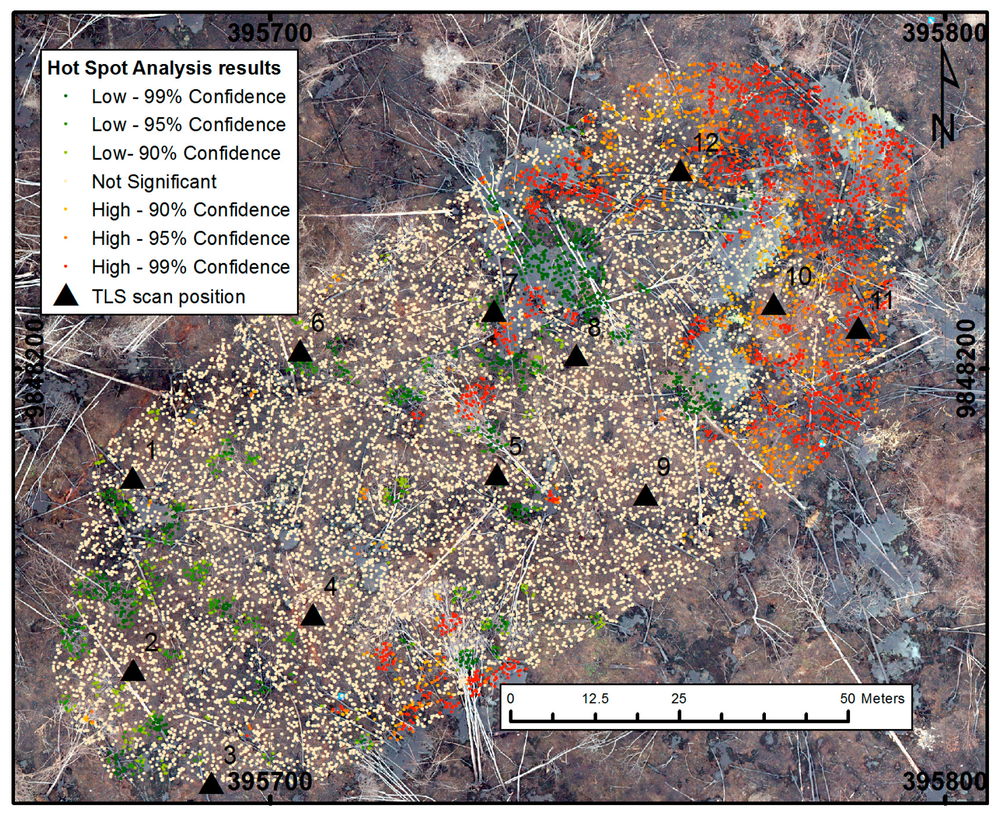
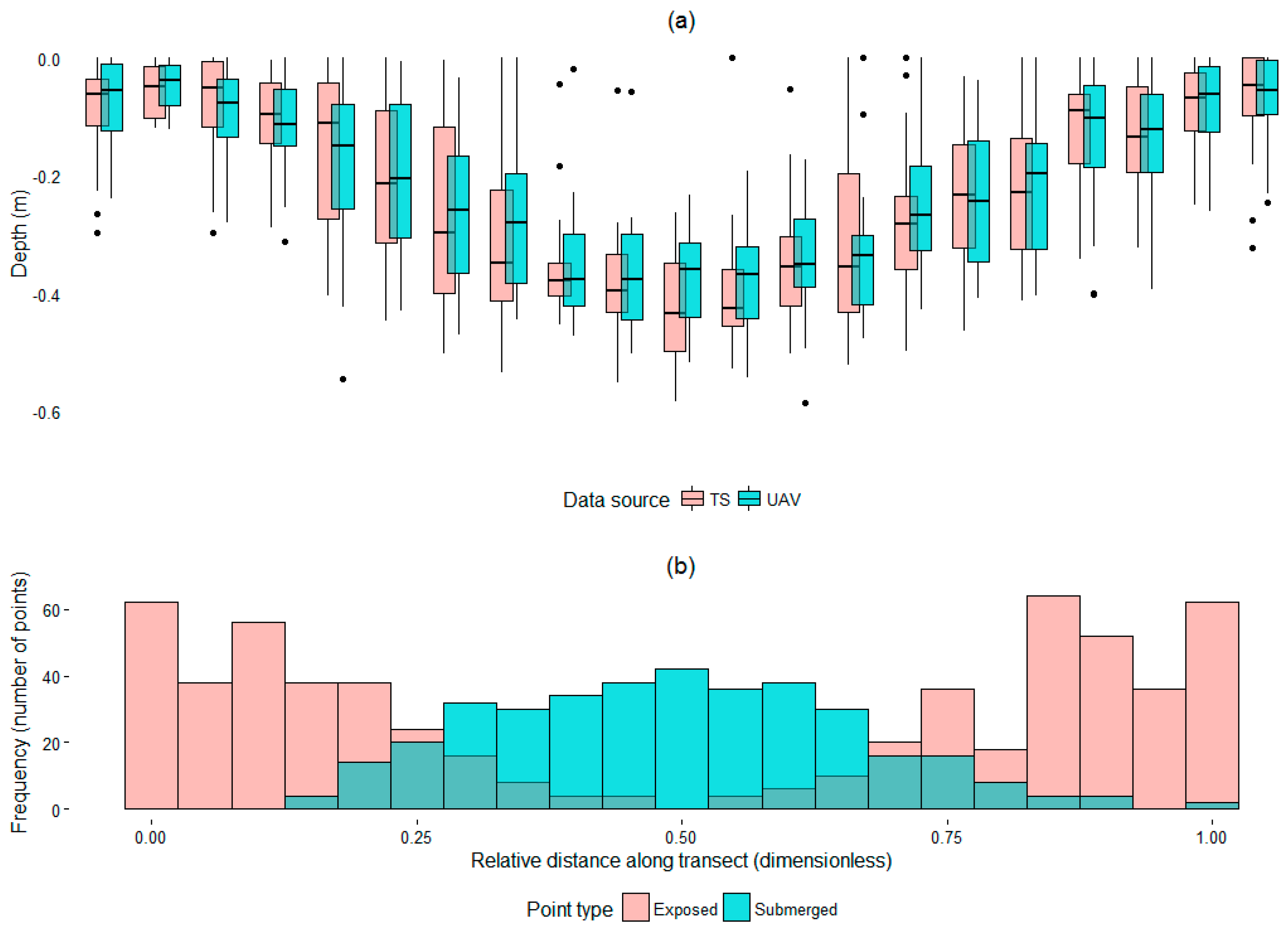
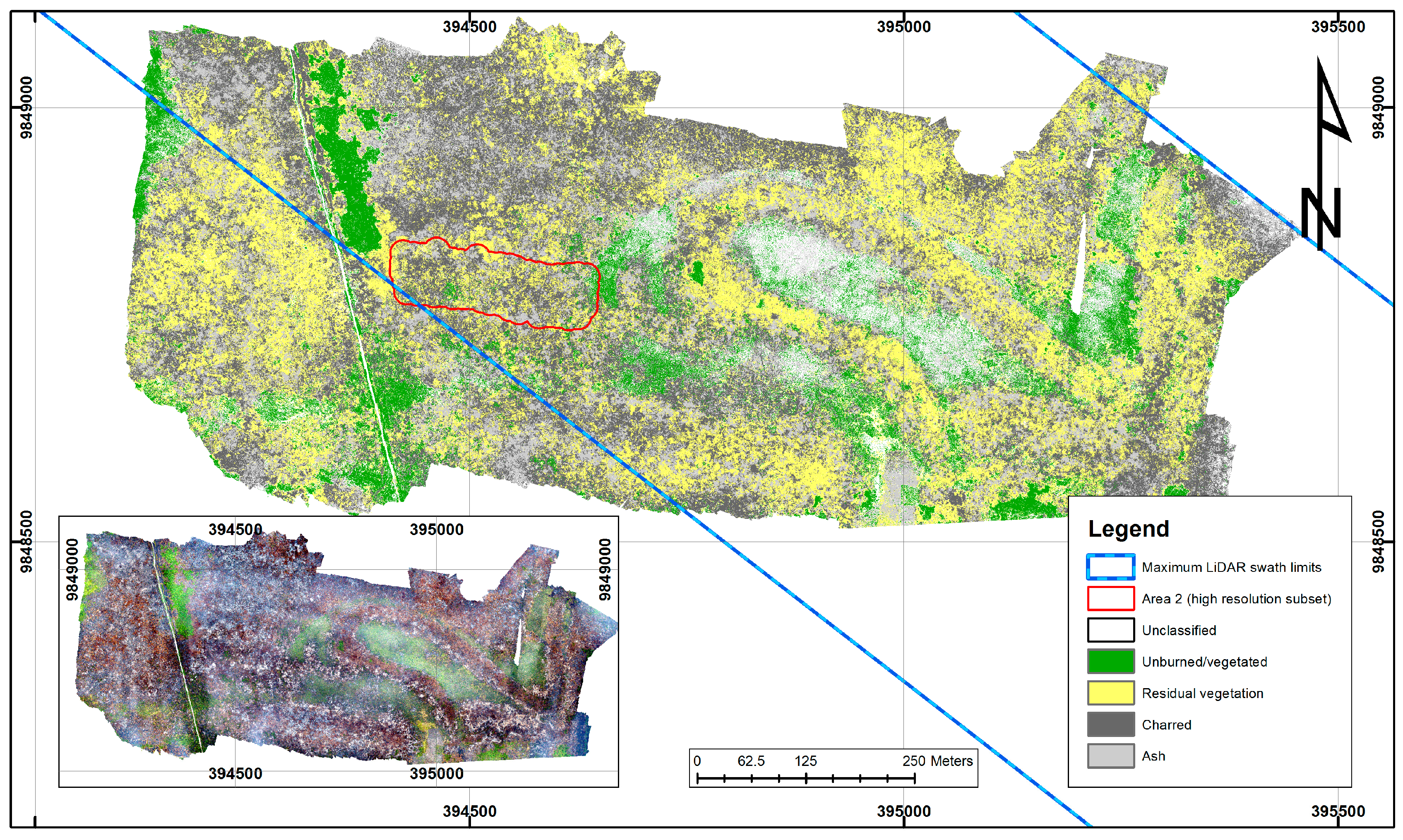
2.3.1. Burn Heterogeneity Assessment (Site 1)

Pre-burn orthomosaic RGB imagery (0.1 m resolution) was collected alongside the LiDAR data during the airborne survey conducted in April 2015 (see Section 2.2.1). For comparison to these, the post-burn photos from the UAV flights were used, being quality-assured, aligned, georeferenced, mosaicked and exported in Agisoft Photoscan Professional v1.2.4 prior to analysis. Site 1 imagery was registered using GCP locations acquired by a Trimble XR differential GPS and location data were post-processed in Trimble Pathfinder Office. Both the pre- and post-burn orthomosaics were classified into different land cover types using maximum likelihood classification (in ENVI v5.1). The pre-burn image classes were live vegetation, residual (dead) vegetation (appearing senesced), bare soil and unclassified (outside of the 5% probability threshold). The post-burn orthophoto classes were visually delineated using training samples identified as vegetation, residual vegetation (dead vegetation, appearing senesced or charred), charred peat (blackened, dry peat), ash and unclassified (outside of the 5% probability threshold). To assess classification accuracy, a spatially randomized subset of pixels was classified using the pre-burn RGB image from the LiDAR survey, and the 0.1 m resolution orthophoto of Area 2 from the UAV survey (Figure 4). A confusion matrix was returned by comparing these control areas with the original pre- and post-burn classifications.

2.3.2. DTM Production (Site 2)

Before performing photogrammetric operations, GNSS rover and base data were post-processed in Leica Geo office v8.3 using the base data as a reference position, precise ephemeris data (from Institut Géographique National (IGN) Global Data Centre and IGS International GPS service for Geodynamics) and four online Precise Point Positioning (PPP) services. These target positions form the GCPs for model registration, and CPs for model accuracy assessment.

The twelve TLS point clouds aligned with a total RMSE of 0.03 m and were registered to UTM 48S projection. The clouds were then combined and exported as one and resampled to 0.05 m resolution. All processing was performed in Riegl Riscan Pro v2.6.2 (64 bit). In total, 8667 UAV photos were used for point cloud production in Agisoft Photoscan Professional v1.2.4. Photoscan was used because it produces the most accurate surface models, and can deal with shadows better than other SfM packages [23]. The workflow recommended by the manufacturers was followed (also see Table 2 in [38]), and where possible, the same GCPs were used to georectify each model (one target was selected as a GCP per 20 m × 20 m grid cell of the survey site). An orthophoto, DTM and point cloud were produced for each flight altitude and camera angle. Point clouds were always decimated (from upwards of 300 million points to ~30 million) so they could be processed within reasonable time scales.

UAV and LiDAR point clouds were filtered for ground points using the LAStools suite [39]. LAStools ground extraction algorithm is based on an iterative grid simplification and has been previously effective in producing DTMs from LiDAR in a Mediterranean forest environment [40,41], and has been applied to dense point clouds produced from UAV SfM in densely forested environments, albeit with limited success because SfM techniques do not easily penetrate overlying vegetation [42]. However, in this study, UAV SfM was not used to survey densely vegetated unburned areas.

Four DTMs are produced for Site 2: a pre-burn DTM from LiDAR data (DTM_LiDAR), a modeled pre-burn surface derived from interpolation of high elevation points as derived from the post-burn DTM_UAV (DTM_IDW), a post-burn DTM from UAV data only (DTM_UAV) and a control DTM from TLS data (DTM_TLS). For DTM_IDW and DTM_UAV, point clouds were clipped 1 m above and below the mean elevation of the ground point cloud to remove outlier points. DTMs were produced by filtering by elevation minima at 1, 5, 10 m for both UAV and LiDAR ground point clouds, and additionally at 0.5 and 0.1 m for the UAV and 20 m for the LiDAR point clouds. These were produced in Cloudcompare v 2.6.2.

Using the post-burn DTM_UAV with the highest overall accuracy (35 m_O,

Table 3. Results from the three accuracy assessments. For each assessment, the most accurate UAV flight is marked in bold.

GNSS Control Point Comparison (vs. DTMUAV)
		XY (m)			Z (m)			XYZ (m)
Flight ID	Number of Points	Bias (m)	St Dev (m)	RMSE (m)	Bias (m)	St Dev (m)	RMSE (m)	Bias (m)	St dev (m)	RMSE (m)
30 m_N	58	0.028	0.020	0.034	−0.012	0.041	0.043	0.049	0.024	0.054
30 m_O	68	0.032	0.022	0.038	−0.001	0.038	0.038	0.047	0.027	0.054
35 m_N	75	0.026	0.020	0.033	−0.001	0.042	0.042	0.044	0.029	0.053
35 m_O	69	0.025	0.018	0.031	−0.009	0.039	0.040	0.043	0.026	0.051
40 m_N	72	0.026	0.021	0.031	−0.004	0.038	0.038	0.043	0.027	0.051
40 m_O	74	0.023	0.020	0.030	−0.005	0.037	0.037	0.040	0.027	0.048
50 m_N	71	0.025	0.020	0.032	−0.003	0.037	0.037	0.041	0.026	0.049
60 m_O	69	0.025	0.020	0.032	−0.003	0.036	0.036	0.040	0.027	0.048
TLS Data Comparison
CloudUAV to DTMTLS Comparison					DTMUAV to DTMTLS Comparison
Flight ID	Number of Points	Bias (m)	St Dev (m)	RMSD (m)	Number of Points	Bias (m)	St Dev (m)	RMSE (m)	Overall RMSE (m)
30 m_N	296,401	−0.022	0.104	0.106	13,703	0.042	0.086	0.096	0.106
30 m_O	1,916,595	−0.044	0.110	0.118	13,703	0.027	0.089	0.092	0.118
35 m_N	1,026,498	0.016	0.097	0.098	13,703	0.030	0.108	0.112	0.099
35 m_O	3,688,289	0.020	0.087	0.089	13,703	0.027	0.086	0.090	0.089
40 m_N	3,111,338	−0.065	0.112	0.129	13,703	0.038	0.129	0.134	0.130
40 m_O	1,042,611	0.003	0.137	0.137	13,703	0.015	0.083	0.084	0.136
50 m_N	928,771	0.017	0.102	0.103	13,703	0.023	0.097	0.100	0.103
60 m_O	923,817	0.041	0.129	0.135	13,703	0.004	0.086	0.086	0.135

), a pre-burn DTM was created using an inverse distance weighting interpolation technique of local elevation maxima taken at points surrounding the pits. This was performed in ArcMap 10.3.3 by firstly gap filling the patchy DTM_UAV, then creating a flow direction raster, followed by the “basin” tool. The basin tool is normally used to delineate drainage basins from DTMs by connecting cells into common pour points. It can be used in this context because fire burns away most of the peat around the base of trees, and so creates pits that have a similar form to basins. Each basin was vectorised and the vertex points around the basin edges were used to extract elevation values from the post-burn DTM_UAV. These point elevation values represent “local maxima”, and were interpolated using inverse distance weighting (which has been demonstrated to be a good surface reconstruction technique by [15]) using default parameters. DTM_IDW was produced at 10 m resolution, and its accuracy was assessed against the post-burn DTM_LiDAR.

2.3.3. DoB Accuracy Assessments

The total station topographic measurements are unbiased by water and are used to assess DTM accuracy under water. A 25 cm buffer around each total station measurement point was used to extract the mean elevation value from DTM_UAV (to account for a slight horizontal misalignment between total station and UAV datasets) and compared to the total station point elevation. Residuals of exposed and submerged points were statistically tested using a Welch’s t-test (in RStudio v0.99.879). Pit depth was analysed in relation to the highest point of each transect. Three accuracy assessments of UAV-derived DTM data were made. Firstly, comparing DTM_UAV with GNSS control points (X, Y and Z). Secondly, comparing raw UAV point clouds with DTM_TLS (X, Y, Z). Thirdly, comparing both DTM_UAV and DTM_TLS (Z only because comparisons are made at randomly located X, Y points). Accuracy is assessed by calculating the root mean square error (RMSE) bias (1). Where point data are not available (comparing point cloud to DTMs), the root mean square deviation (RMSD) is calculated using bias and scatter (2) [38]. Overall RMSE of all models combined can be calculated using (3):

$$\overline{x}={\displaystyle \sum }_{i=1}^n\frac{\left({\widehat{z}}_i-z_i\right)}{n}$$

(1)

$$\mathrm{RMSD}=\sqrt{({\sigma }^2+{\overline{x}}^2})$$

(2)

$$\mathrm{Overall}\mathrm{RMSE}=\sqrt{{\displaystyle \sum }_{i=1}^n\frac{\left(n\times {{\mathrm{RMSE}}_i}^2\right)}{n}}$$

(3)

where z and ${\widehat{z}}_i$ are the observed and estimated elevations, $\overline{x}$ is the bias, $\sigma$ is the standard deviation, and n is the sample size.

To examine the effects of flight altitude and camera orientation, non-parametric Kruskal–Wallis rank sum tests were performed on the XY, Z, and XYZ residuals, and pairwise differences were tested at 95% confidence interval.

DTM_TLS was interpolated from ground points at 0.05 m resolution and bias was −0.019 m when compared to 31 GNSS points, and so the DTM_UAV was corrected accordingly. TLS and UAV point cloud residuals were calculated in Cloudcompare v.2.6.2. Eight DTM_UAV were compared to the DTM_TLS at 13,073 spatially randomised points. Finally, in the most accurate DTM_UAV, error spatial autocorrelation and clustering were assessed using the spatial autocorrelation (Global Moran’s I) and hot spot analysis (Getis-Ord Gi*) tools respectively (ArcMap 10.3).

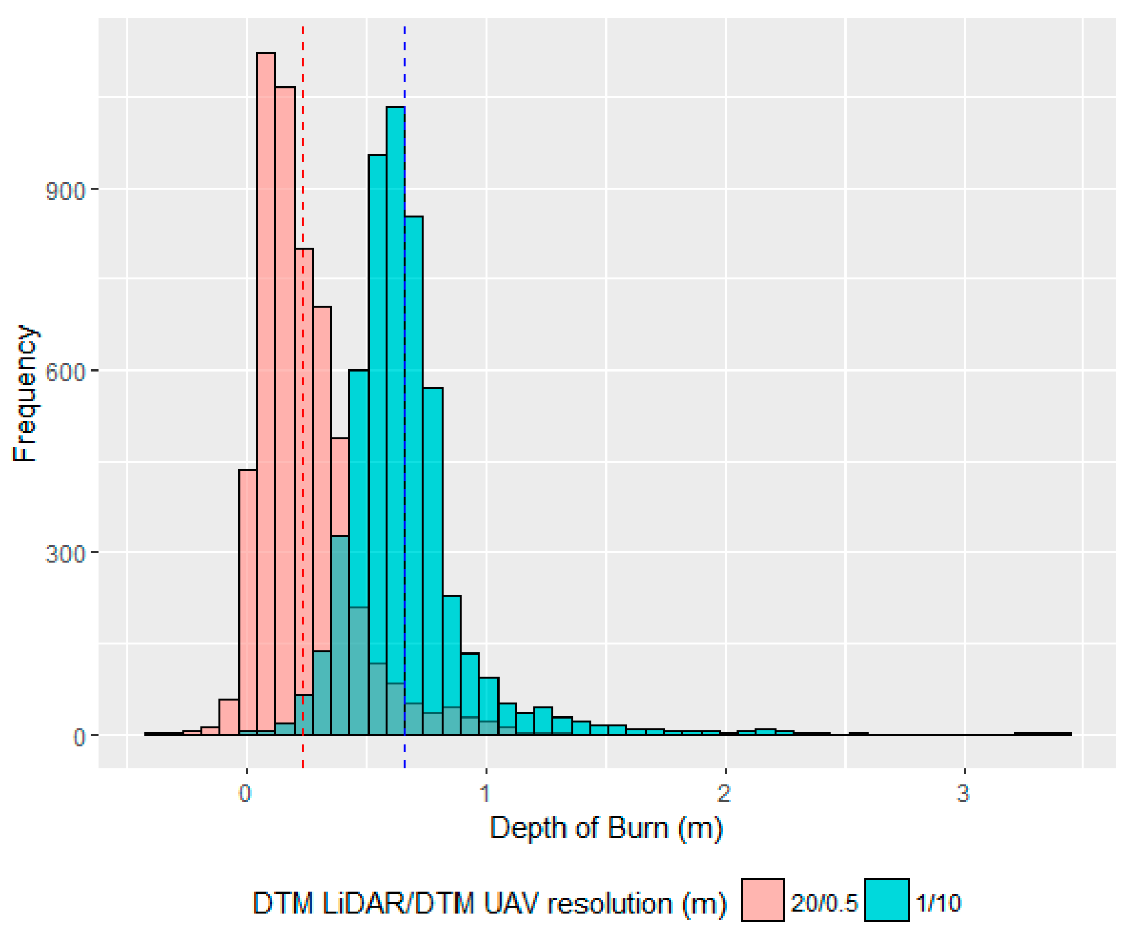
2.3.4. Peat Depth of Burn from DTMs

The DTM_UAV from survey 35 m_O was used to produce DoB estimates because overall it was the most accurate DTM (Table 3). DTM_UAV and DTM_LiDAR were aligned vertically in an unburned area next to a small wooden house that survived the fire. Elevation differences were calculated between pre-burn DTMs (DTM_LiDAR and DTM_IDW), and the post-burn DTM_UAV along 15 East–West transects spaced 10 m apart, at points 1 m apart [9]. Points were delineated as being on burned forest (n = 5305) by visually inspecting both pre- and post-fire aerial photographs.

3. Accuracy Assessment Results

3.1. Classification of Optical UAV and Airborne LiDAR Datasets (Site 1 Only)

Confusion matrices that were produced for both the pre- and post-burn RGB classifications (from the LiDAR and UAV) had an accuracy of 96% and 95% (Kappa coefficient = 0.93 and 0.93), based on comparison to high resolution aerial photographs. In total 30,554 and 105,281 visually delineated control pixels were used for the pre-burn and post-burn classification accuracy assessments. For the post-burn classification, Area 2 (1.5 ha) was used to assess the accuracy of Area 1 (56.9 ha) as the image was more detailed owing to the spatial resolution in Area 2 being 10 times higher (Figure 4).

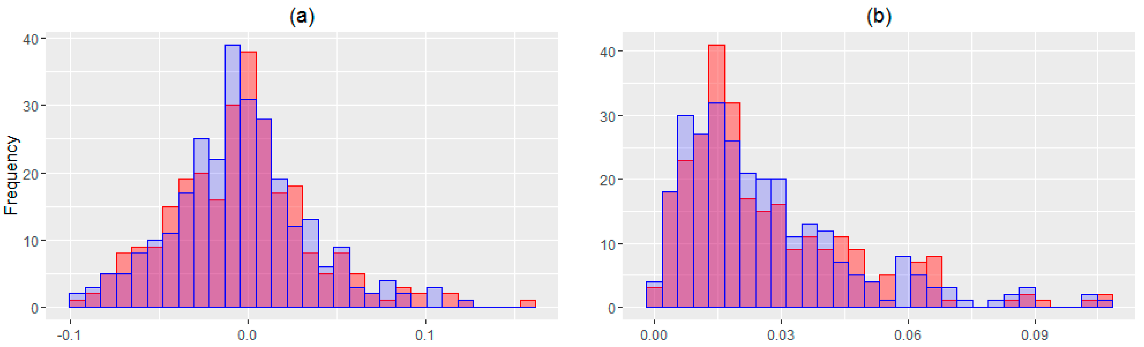
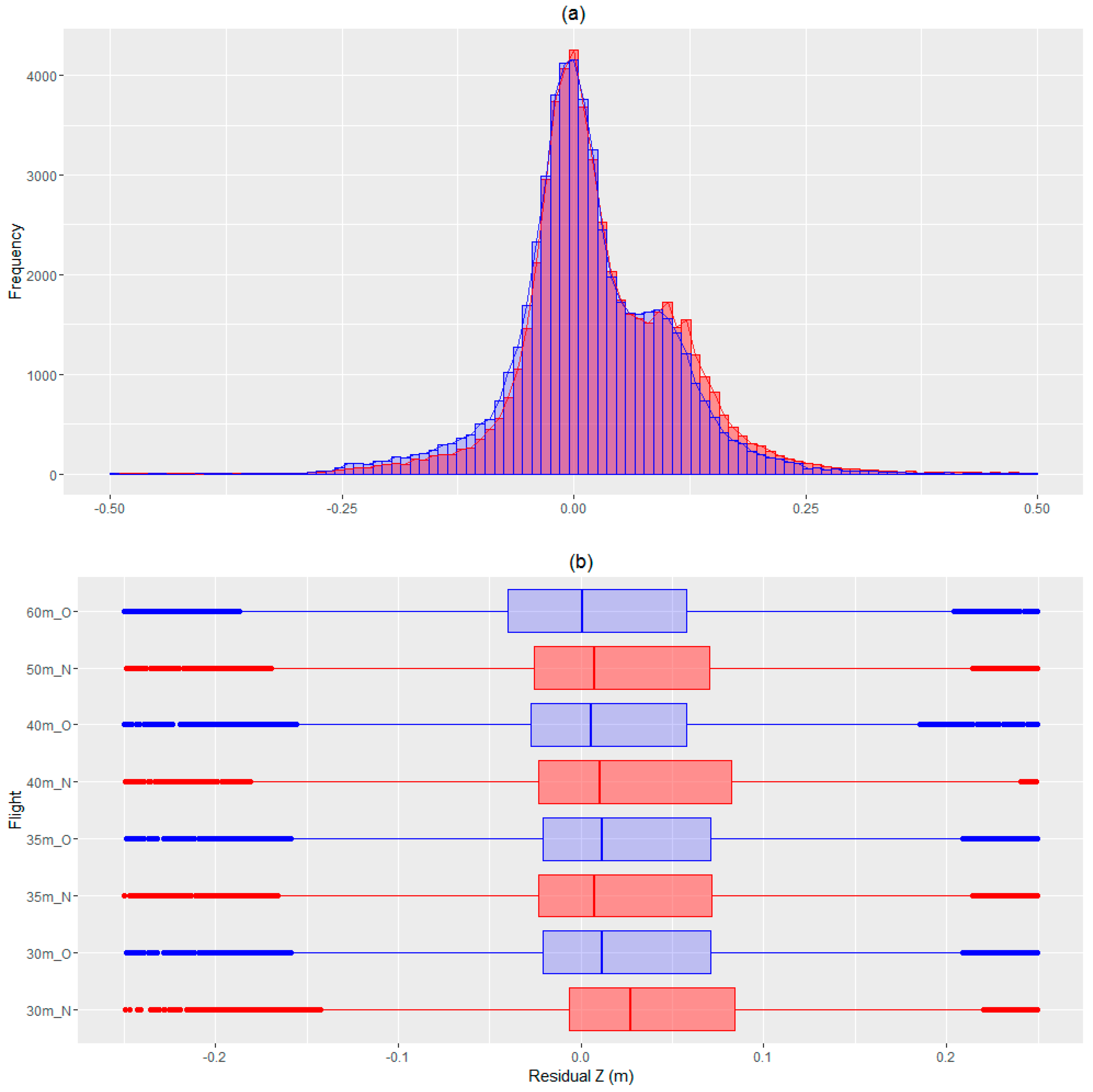
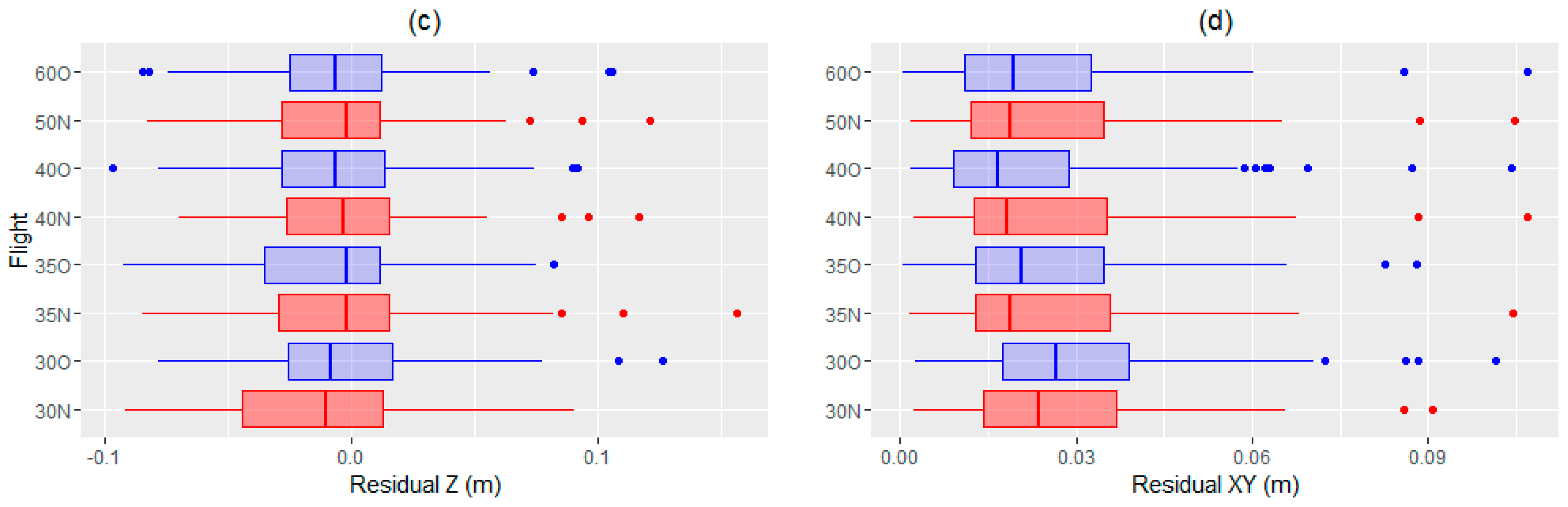
3.2. DTM_UAV Accuracy Assessments

Compared to GNSS-control points, the UAV-derived digital terrain data (DTM_UAV) show little bias in the XY, Z, and XYZ directions (<0.032, <0.012, and <0.049 m respectively; Table 3), and overall small random errors (<0.038, <0.043, and <0.054 m respectively; Table 3). Non-parametric Kruskal–Wallis rank sum tests show no significant difference in residuals as a result of flight altitude (p = 0.318) or camera angle (p = 0.432) (Figure 5, Table 3).

A total of 12,934,320 UAV point cloud data points were compared to DTM_TLS (Table 3). Most ground points are considered very accurate, especially around scans 1–9 (Figure 6, Table 3). In this area, errors are highly auto-correlated (Moran’s Index = 0.61, z-score = 183.2, p < 0.001) and clustered around areas where vegetation is insufficiently filtered out, and in pits filled with water. The most accurate flight was 35 m_O with RMSD = 0.089 m, or 0.07 m when only non-auto-correlated errors are considered.

Survey 60 m_O performed the best when comparing the DTM_UAV with the DTM_TLS (RMSE = 0.086). The oblique camera angle (RMSE = 0.089 m) performed statistically better than the nadir camera angle (RMSE = 0.111 m, H₁ = 487.35, p < 0.001) (Figure 7, Table 3). Flights 30 m_O and 35 m_O were flown at roughly the same altitude (36.4 and 37 m respectively) and the DTMs from both surveys showed little difference (bias = 0.002 m, RMSE = 0.049 m, n = 943,990), demonstrating repeatable results from different surveys.

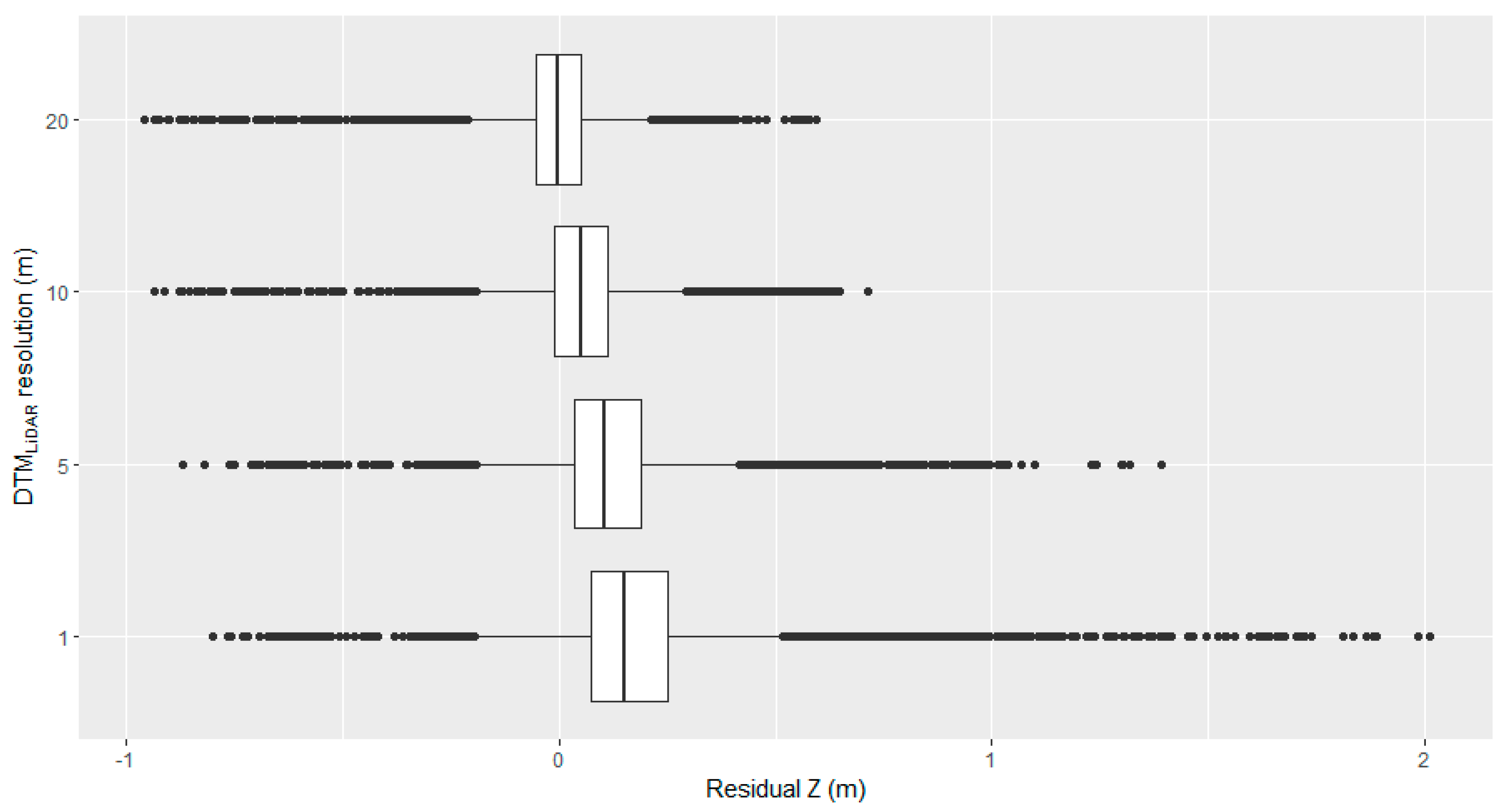
3.3. DTM_IDW Accuracy Assessment

The DTM_IDW was compared to DTM_LiDAR at 1, 5, 10 and 20 m resolution using 5305 points collected along 15 transects, and bias assessed as a measure of accuracy because the mean of the elevation residuals affects emissions estimates, rather than the random error. DTM_IDW is considered to perform well against 10 and 20 m pre-burn DTM_LiDAR (bias = 0.05 and −0.01 m, RMSE = 0.16 and 0.12 m respectively) compared to 1 and 5 m resolution which performed poorly (bias = 0.19 and 0.12 m and RMSE = 0.32 and 0.23 m respectively). This demonstrates that, on average, the modeled pre-burn surface calculated from spatial interpolation of the post-burn UAV imagery (DTM_IDW) accurately replicated the pre-burn heights recorded in DTM_LiDAR (Figure 8 and Figure S1).

3.4. DTM_UAV Accuracy under Water

DTM_UAV was slightly less accurate under water than at non-submerged points (Figure 9). The differences were −0.004 ± 0.062 and −0.012 ± 0.092 m for exposed and submerged points respectively (RMSE = 0.062 and 0.093 m respectively) which was significant (t_284.5 = 2.126, p < 0.05). However, in practice, the difference in bias is considered very small (<0.01 m), and these results imply that the UAV SfM technique is capable of measuring surface topography through shallow water (as in [30]) which is an advantage over laser-based methods.

4. DoB and Combustion Heterogeneity Analysis Results

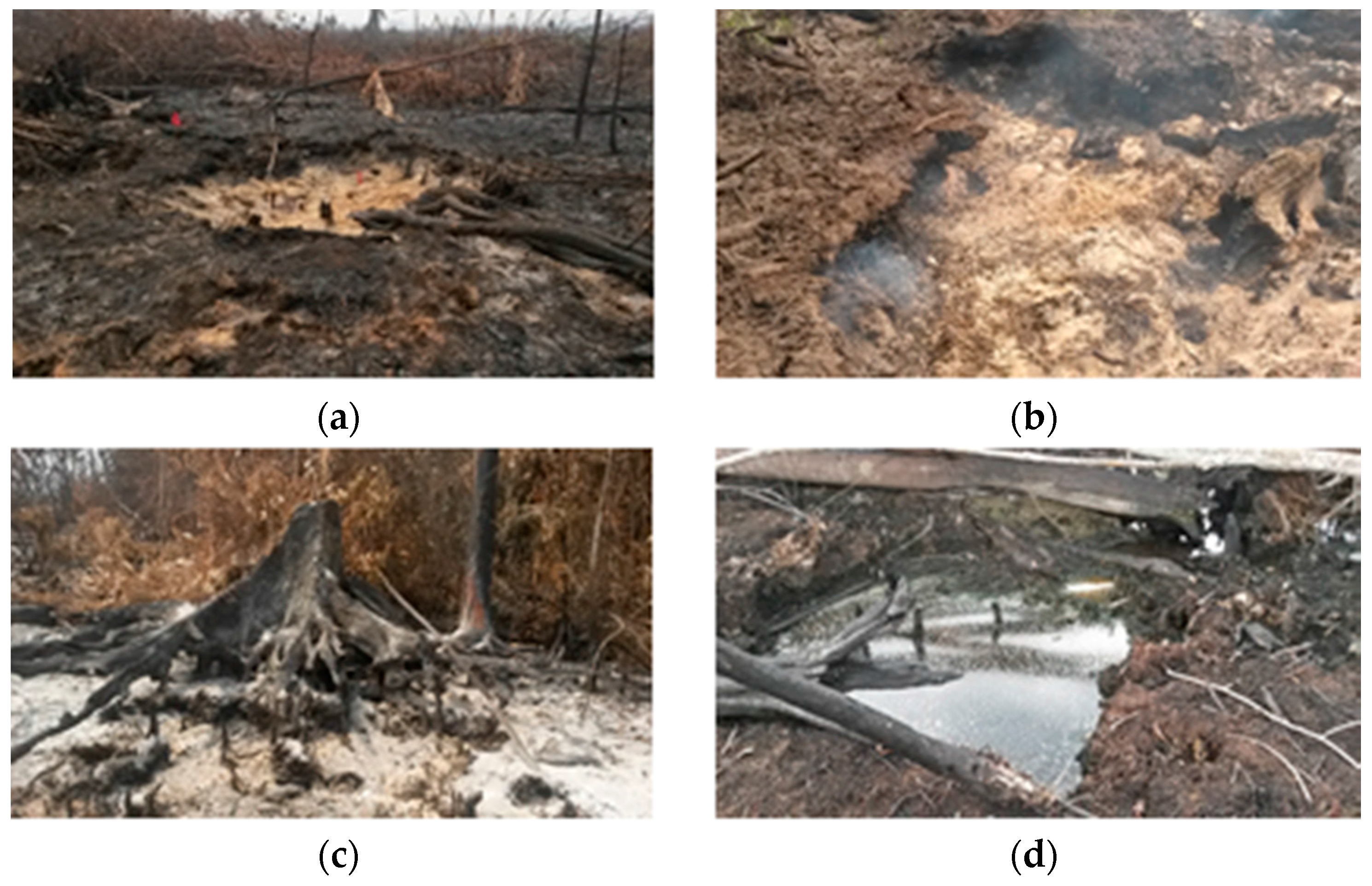
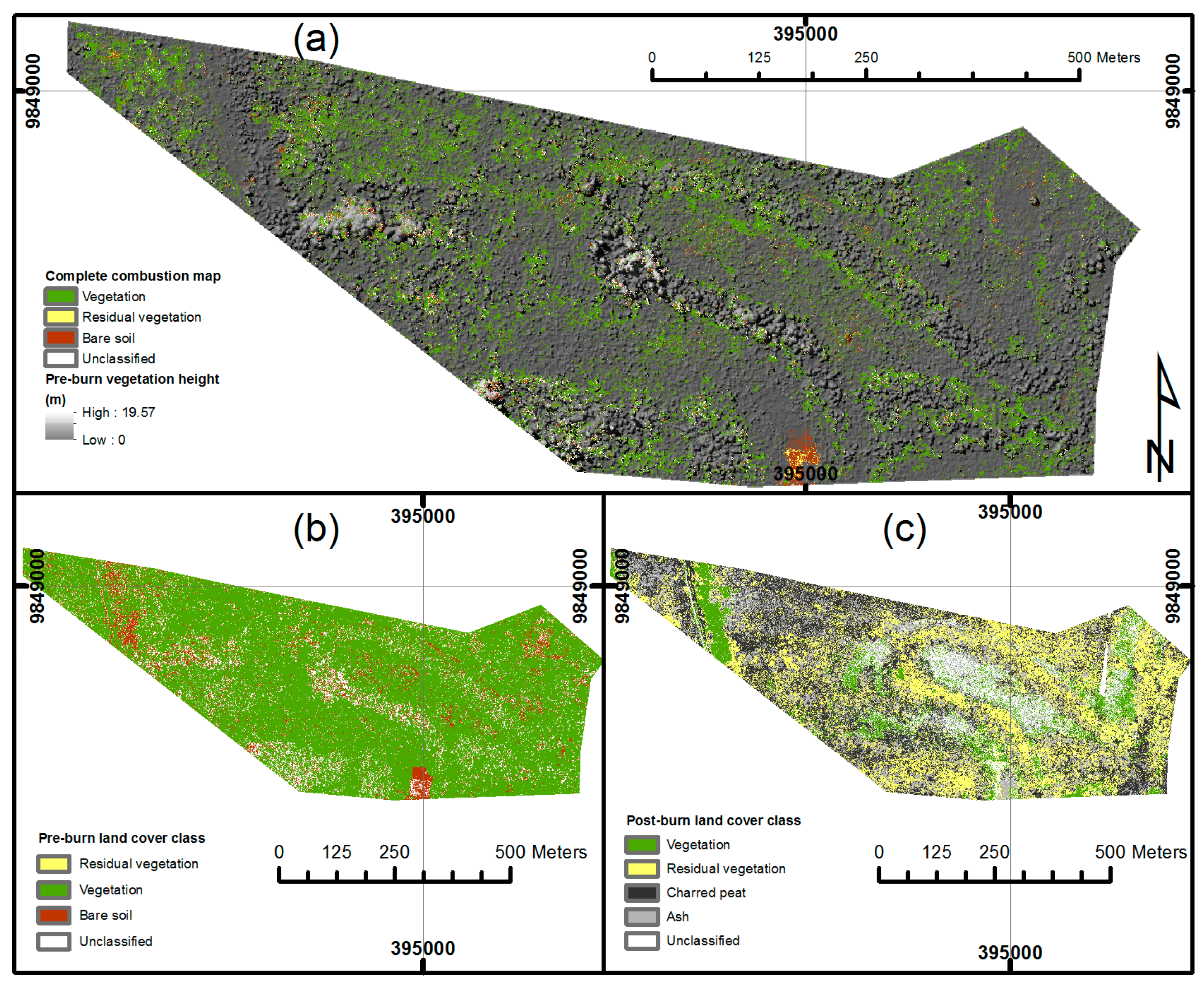
4.1. Combustion Heterogeneity (Site 1)

Here, we report the changes in land cover caused by the fire by comparing pre- and post-burn classifications of site 1: only 21% of the fire affected area was covered in ash (evidence of complete combustion). In the 38 ha area where both pre- and post-burn datasets overlap, of the 6,545,516 pixels classified as completely combusted 79.9%, 9.6%, 8.6%, 1.8% and 0.04% were from vegetation, bare soil, residual vegetation and unclassified classes respectively (Figure 10). While this shows that much of the most complete combustion occurs around the roots of vegetation, other post-burn classes also exhibit somewhat similar burn characteristics (i.e., vegetation was the most prevalent pre-burn class for all post-burn classes at between 77.6% and 84.1%).

The mean pre-burn vegetation height was also calculated for each post-burn class. Residual vegetation seen in the post-burn imagery had the tallest pre-burn vegetation (2.1 ± 2.2 m), followed by post-burn areas of ash (1.8 ± 2.1 m) (Figure 10), char (1.6 ± 1.8 m) and post-burn live vegetation (1.2 ± 0.9 m). Alongside our field observations, this suggests that the areas that are covered in dead residual vegetation after the fire were previously covered in the tallest live vegetation, and that areas of tall vegetation before a fire lead to the most complete combustion (mostly around the base of the vegetation and the roots) during the fire.

4.2. DoB Estimates

Mean estimates of the peat DoB varied widely with DTM spatial resolution (

Table 4. Mean DoB estimates (and σ in brackets) using pre- and post-burn DTMs of different resolutions. Estimates in green are considered overestimates caused by pre-burn vegetation signal, estimates in blue are considered overestimates because of excessive smoothing of the post-burn DTM, estimates in yellow are considered both under and over estimates caused by limited vegetation signal and/or excessive smoothing, and estimates in black are best estimates produced from use of the optimum spatial resolution pre- and post-burn DTMs.

Pre-Burn DTMLiDAR Resolution (m)	Post-Burn DTMUAV Resolution (m)
	0.1		0.5		1		5		10
1	0.44 a	(0.29)	0.43 a	(0.29)	0.33	(0.26)	0.52	(0.27)	0.66	(0.26)
5	0.37 b	(0.24)	0.37 b	(0.23)	0.26	(0.20)	0.45	(0.20)	0.58	(0.20)
10	0.30 c	(0.20)	0.29 c	(0.20)	0.19	(0.16)	0.38	(0.16)	0.51	(0.16)
20	0.24 d	(0.19)	0.23 d	(0.19)	0.13	(0.15)	0.31	(0.16)	0.44	(0.15)
DTMIDW (10 m)	0.25	(0.20)	0.24	(0.20)	0.14	(0.16)	0.32	(0.16)	0.46	(0.16)

^{a, b, c, d} Estimates with the same letter notations are not significantly different.

), and so the most appropriate scale for DoB derivation needs careful consideration. The DTM_LiDAR datasets produced at 1 and 5 m spatial resolutions show considerable high spatial frequency variations (Figure 11 and Figure S1), most likely due to the LiDAR returns being reflected from vegetation (such as tree trunks) rather than from the ground surface itself. Further to this, there is a tendency for the pre-burn elevation data to show local maxima at the same points along a transect where the post-burn elevations show a local minima, and the fact that the deepest burns are around the roots of trees supports helps to explain this. The DTM_LiDAR produced at 10 m spatial resolution shows a reduction in such effects, presumably because at this grid cell size, there are usually some LiDAR returns coming from the ground surface in each cell, and at 20 m the vegetation component of this elevation signal appears fully removed, representing ground topography. Conversely, the post-burn DTM_UAV produced at 0.1 and 0.5 m spatial resolution is more representative of ground topography than at the lower 1, 5 or 10 m spatial resolutions, because at the lower resolutions the deep burn pits are smoothed, the topographic detail induced by the burning is lost, and the mean ground height underestimated. There is no advantage in increasing resolution beyond 0.5 m as there is no significant difference to DTM_UAV at 0.1 m (t = 1.94, df = 10,593, p = 0.05). Therefore, the optimal combination of DTMs for depth of burn analysis are considered to be the 20 m resolution DTM_LiDAR and the 0.5 m resolution DTM_UAV, and the resulting mean depth of burn using these data is 0.23 m, with a 0.19 m standard deviation (Figure 12).

The DoB is 0.25 ± 0.20 m (mean ± one standard deviation) when DTM_LiDAR at 20 m resolution is replaced with DTM_IDW, and while the mean DoB estimates for DTM_IDW and DTM_LiDAR are statistically different (t = 2.91, df = 10,595, p < 0.05), in practice there is, on average, only 0.01 m difference.

5. Emissions Estimates

Method for Calculating Emissions Estimates

We calculated emissions estimates from these peatland burns using the ‘bottom-up’ approach popularised by [43] and used in the Intergovernmental Panel on Climate Change (IPCC) Equation (4). This requires an estimate of the burned area and also depth of burn (DoB), in order to calculate the volume of peat burned [11].

$$L_{fire}=A\times B_D\times DoB\times C_F\times G_{ef,i}\times {10}^{-3}$$

(4)

where L_fire is the quantity of CO₂ or non-CO₂ gas emitted by the fire (tonnes), A is the burned area (5.2 ha), B_D is dry bulk density (0.106 g∙cm⁻³ from [35]), DoB is depth of burn (0.23 m), C_f is the combustion factor (assumed to be 1, dimensionless), and G_ef is the biome specific emission factors for CO₂-C, CO-C and CH₄-C (434.7, 109.3 and 5.6 gC∙kg⁻¹ dry mass burned respectively, from [3]).

Uncertainty in the emissions estimates were assessed using the standard error propagation approach, firstly assessing the uncertainty in the mean DoB estimate:

$$\delta DoB=\frac{\sqrt{\delta DT{M_{UAV}}^2+\delta DT{M_{LiDAR}}^2+\delta DT{M_{unburned}}^2}}{\sqrt{n}}$$

(5)

where $\delta DT{M}_{UAV}$ and $\delta DT{M}_{LiDAR}$ are the uncertainties of DTM_UAV and DTM_LiDAR (m), and $\delta DT{M}_{unburned}$ is the standard deviation of the DTM_UAV, DTM_LiDAR differences (m) in the unburned area after any biases were removed and n is number of sampled points.

The uncertainties in the final emissions were then estimated via the following equation:

$$\delta L_{fire}=L_{fire}\times \sqrt{{\left(\frac{\delta DoB}{DoB}\right)}^2+{\left(\frac{\delta B_D}{B_D}\right)}^2+{\left(\frac{\delta G_{ef,i}}{G_{ef,i}}\right)}^2+{\left(\frac{\delta A}{A}\right)}^2}$$

(6)

where δ is the random error of the estimated term. This method is in line with [10].

Peat bulk density was taken as 0.106 ± 0.028 g∙cm⁻³ in Jambi [35], and for emissions factors we used the first field-derived emission factors collected for Indonesian tropical peat fires by [3], assessed during the El Niño-exacerbated fires of 2015. For CO₂, CH₄ and CO, these EFs are 1594 ± 61, 7.4 ± 2.3, and 255 ± 39 g·kg⁻¹ respectively for peat-only emissions. Based on the assumption that combustion completeness is 1 for our site across the 5.2 ha burned area (because we explicitly measured depth of burn rather than stating that a certain fraction of the peat available at each location was burned), the total mass of peat consumed is estimated as 1271 tonnes, distributed as to 106.0 ± 28.3 tCO₂-C·ha⁻¹ (tonnes of C emitted per hectare as CO₂) 26.6 ± 8.3 tCO-C·ha⁻¹, and 1.4 ± 0.4 tCH₄-C·ha⁻¹, totaling 134.0 ± 29.4 tC·ha⁻¹ for peat only. Uncertainties in DoB are responsible for <1% of the quantified uncertainty, with bulk density and emissions factor uncertainties smaller contributions (around 37% and between 0.7% (for CO₂) and 50% (for CH₄) respectively. When calculating emissions using DTM_IDW, overall uncertainty is increased slightly owing to a higher uncertainty caused by the 0.12 m RMSE between DTM_IDW and DTM_LiDAR.

6. Discussion

We have presented a structure from motion (SfM) approach for spatially mapping peatland depth of burn (DoB), based around post-fire imagery collected via a small, affordable UAV. To our knowledge, this is the first time such an approach to digtial terrain model (DTM) generation has been applied to assess DoB. We confirmed the versatility, accuracy and optimium setup for the approach; with suitable imagery for deriving surface DTMs collected at a variety of flying altitudes (up to 70 m) and camera angles. DTMs showed accuracies better than 5 cm compared to ground survey measures, comparable to that of airborne LiDAR (e.g., 7–15 cm for [6,16]). By comparing pre- and post-burn DTMs of the same 5.2 ha area, peatland DoB was mapped across a degraded peatland (not previously burned) and mean DoB assessed as 0.23 m with <1% uncertainty. The standard deviation of the DoB measures is 0.19 m, indicating wide DoB variations, and maximum DoB extended beyond 1 m in some locations. This range is similar to estimates for forests that have only burned once [15], but less than the prior estimate provided by [9] (0.33 ± 0.19 m) for essentially the same biome. The deepest burns occur around the roots of vegetation which is confirmed in Figure 11 and Figure S1 where the some of the highest pre-burn peaks occur in the same location at the lowest post-burn pits, and by the combustion heterogeneity analysis based on analysis of the RGB imagery collected from the UAV (Section 4.1). These DoB estimates translate to a carbon emissions estimate of 134 ± 29 tC·ha⁻¹, which is slightly more than the estimate from [15] for “first fires” in these types of biome, and improves upon previously reported uncertainties of up to 32% [1,9].

Although we used airborne LiDAR data to create our pre-burn DTM, we have also demonstrated that spatial interpolation of the post-burn UAV data alone can be used to create a pre-burn surface very similar in charcter to the actial LiDAR-derived pre-burn DTM (e.g., −0.01 m bias at 10 m resolution). When DTM_LiDAR is substituted for DTM_IDW the ‘post-burn only’ data still provides an overall uncertainty of <0.01 m in mean DoB asssessment. With further investigation, this method could eliminate the need for pre-burn LiDAR data, which are often not available in studies estimating depth of burn at new fire sites [9,15].

Our combustion heterogeneity analysis demonstrates around 21% of the large shrubby peatland area was affected by complete combustion, and that maximum combustion occurs around vegetation roots, where the deepest burns are likely to occur, creating deep burn pits.

This is the first study to difference pre- and post- burn DTMs of the same area in tropical peat burns to assess emissions estimates. Previously, [9] compared post-fire average elevation in burned areas with adjacent unburned area, and [15] modeled a pre-burn surface using interpolation of adjacent unburned areas. While our study area is much smaller than these previous efforts due to flying limitations of the UAV, it offers several benefits. Firstly, the derived DTM_UAV is of very high resolution (0.1–0.5 m), and highly precise (with random errors much smaller than in [9,15]). Secondly, the UAV can be deployed with very little expense, planning, or effort compared to a full airborne LiDAR campaign. Finally, the UAV system is capable of producing a pre-burn DTM (DTM_IDW) which is comparable to the pre-burn DTM_LiDAR (bias = 0.01 m). Here, the bias is more important than the random error because mean depth is used to calculate the volume of peat burned, and random error is cancelled out as long as elevation distribution is normal.

We have examined the effects of SfM spatial filtering on both pre- and post-burn datasets. By filtering each DTM using the lowest classified ground point per grid cell, we found it possible to create the required peat surface DTMs. In the pre-burn profile in Figure 11, the green area shows how higher resolution filtering of DTM_LiDAR (1–10 m) seems to capture vegetation (as seen by the abrupt peaks) rather than ground height values, which are best characterised by 20 m resolution DTM_LiDAR. This suggests that processing pre-burn LiDAR data at high resolution in densely vegetated areas may overestimate pre-burn elevation because true ground points are less likely to be returned in smaller grid cells [44], as could be the case in [9,15]. On the contrary, a larger grid cell flattens and underestimates the post-burn DTM because interpolation may exclude much of the remaining peat. In Figure 11, DTM_UAV captures true peat microtopography best at 0.1 and 0.5 m because the filtering effect of lower resolution DTMs excessively smooths the surface topography (as seen by the red dotted/dashed lines in the red area). It is thus important to find a balance between filtering out the impact of residual vegetation (which is improved with larger grid cells in heavily vegetated pre-burn datasets) and maintaining topographic detail in open post-burn datasets. Where possible, filtering algorithms should be applied to point cloud datasets, however the results should be examined carefully to ensure the impact of pre-burn vegetation is adequately filtered out in the resulting surface DTM.

While we have quantified known uncertainties, there remains a very important uncertainty that is not able to be considered here. Despite using recommended algorithms and techniques, there is no guarantee that the derived ground points, output after filtering, actually do represent ground height, rather than the top of a thick surface vegetation layer. The study area was heavily vegetated before the fire, with tall canopy trees (35 m) interspersed with dense ground shrubs. It is not possible to estimate whether LiDAR ground return did in fact come from the ground surface and not from the top of the surface vegetation layer. Previous accuracy assessments of DTM retrieval show their lowest random error of 0.12/0.19 m in unburned/burned tropical peat forest [15], 0.58 m in unburned tropical forest as a result of incomplete canopy penetration [45], and up to 0.26 m in densely vegetated wetlands [46]—values that are in some cases larger than the DoB estimates made in this study. We have no way of quantifying pre-burn DTM error in our study area because there were no control point measurements taken beneath vegetation at the time. Some existing studies estimating DoB have also failed to quantify this uncertainty [9], and therefore may suffer from a biased pre-burn surface leading to an overestimated DoB. This remains an obvious research question to be answered within the context of DoB measurements from LiDAR.

It took a total of 18 person-hours to set up the ground control points (GCPs) needed for the UAV survey, and a further 2 person-hours were needed to fly the complete survey. The TLS scans required a total of 48 person-hours. Furthermore, the UAV weighs 4 kg with its carry case and batteries, compared to over 30 kg for the TLS. In terms of out-right costs, the TLS costs >USD 110,000 (United States Dollar) compared to ~USD 2000 for the UAV and camera and educational software licenses (however, the UAV system requires either a GNSS for GCP registration, these can be rented from survey companies, or bought second hand for <USD 7500). The cost ($) multiplied by person effort (h) and weight (kg) (user inputs), divided by usable coverage area (m²) (outputs) equates to the UAV survey requiring 0.01 $·kg·h·m⁻² compared to the TLS which requires 13.01 $·kg·h·m⁻². Furthermore, because the UAV survey is conducted from above, there are fewer gaps in the DTM which require interpolation. Finally, the UAV has the added benefit over all LiDAR systems that it can (albeit more roughly) capture topography through water. Therefore, the UAV system can provide an efficient, cheap and flexible alternative to terrestrial laser scanning systems for point cloud retrieval in rugged, remote and challenging conditions in burned peat swamp forests. While UAV coverage might be much lower than airborne LiDAR, this method might be the only affordable option to REDD+ practitioners without large budgets.

7. Conclusions

This paper examines burn scar characteristics in great detail, showing that, within burned areas, peat combustion is heterogeneous, mainly concentrating around the roots of vegetation. We contribute a new dataset on tropical peatland topography, demonstrate a novel, low-cost and versatile method for surveying burned areas using a simple and accessible UAV system, and provide both DoB estimates for first-time fires in degraded peat swamp forest with less uncertainty than previous studies. This study also suggests that previous methods over-estimate DoB for two reasons; they do not capture the true pre-burn ground height because of vegetation obscuring the ground, and the post-burn topographic detail is lost if the grid cell resolution is too low (e.g., 10 m). Error propagation in emissions estimates is important because (e.g., in our uncertainty analysis) every 1 cm error in depth of burn estimate equates to approximately a 2.5% difference in the overall carbon emissions estimate or ~3 tC·ha⁻¹. In order for schemes such as REDD+ to gain momentum in tropical countries, it is important that carbon emissions uncertainties are adequately constrained to provide measurable and verifiable net carbon emissions benefits. Our methodology could thus provide important inputs to these processes, along with IPCC-compatible emissions estimates.

References

1. Page, S.E.; Siegert, F.; Rieley, J.O.; Boehm, H.-D.V.; Jaya, A.; Limin, S. The amount of carbon released from peat and forest fires in Indonesia during 1997. Nature 2002, 420, 61–65. [Google Scholar] [CrossRef] [PubMed]
2. Van der Werf, G.R.; Randerson, J.T.; Giglio, L.; Collatz, G.J.; Mu, M.; Kasibhatla, P.S.; Morton, D.C.; DeFries, R.S.; Jin, Y.; van Leeuwen, T.T. Global fire emissions and the contribution of deforestation, savanna, forest, agricultural, and peat fires (1997–2009). Atmos. Chem. Phys. 2010, 10, 11707–11735. [Google Scholar] [CrossRef] [Green Version]
3. Huijnen, V.; Wooster, M.J.; Kaiser, J.W.; Gaveau, D.L.A.; Flemming, J.; Parrington, M.; Inness, A.; Murdiyarso, D.; Main, B.; van Weele, M. Fire carbon emissions over maritime southeast Asia in 2015 largest since 1997. Sci. Rep. 2016, 6, 26886. [Google Scholar] [CrossRef] [PubMed]
4. Usup, A.; Hashimoto, Y.; Takahashi, H.; Hayasaka, H. Combustion and thermal characteristics of peat fire in tropical peatland in Central Kalimantan, Indonesia. Tropics 2004, 14, 1–19. [Google Scholar] [CrossRef]
5. Rein, G. Smouldering Fires and Natural Fuels. In Fire Phenomena and the Earth System; Belcher, C.M., Ed.; John Wiley & Sons: Oxford, UK, 2013; pp. 15–33. [Google Scholar]
6. Davies, G.M.; Gray, A.; Rein, G.; Legg, C.J. Peat consumption and carbon loss due to smouldering wildfire in a temperate peatland. For. Ecol. Manag. 2013, 308, 169–177. [Google Scholar] [CrossRef] [Green Version]
7. Ashton, C.; Rein, G.; Dios, J.D.; Torero, J.L.; Legg, C.; Davies, M.; Gray, A. Experiments and Observation of Peat Smouldering Fires. In Proceedings of the International Meeting of Fire Effects on Soil Properties, Barcelona, Spain, 31 January–3 February 2007.
8. Rein, G.; Cleaver, N.; Ashton, C.; Pironi, P.; Torero, J.L. The severity of smouldering peat fires and damage to the forest soil. Catena 2008, 74, 304–309. [Google Scholar] [CrossRef]
9. Ballhorn, U.; Siegert, F.; Mason, M.; Limin, S. Derivation of burn scar depths and estimation of carbon emissions with LiDAR in Indonesian peatlands. Proc. Natl. Acad. Sci. USA 2009, 106, 21213–21218. [Google Scholar] [CrossRef] [PubMed]
10. Global Forest Observations Initiative. Integrating Remote-Sensing and Ground-Based Observations for Estimation of Emissions and Removals of Greenhouse Gases in Forests: Methods and Guidance from the Global Forest Observations Initiative; Group on Earth Observations: Geneva, Switzerland, 2014. [Google Scholar]
11. Hiraishi, T.; Krug, T.; Tanabe, K.; Srivastava, N.; Jamsranjav, B.; Fukuda, M.; Troxler, T. 2013 Supplement to the 2006 IPCC Guidelines for National Greenhouse Gas Inventories: Wetlands; Intergovernmental Panel on Climate Change (IPCC): Geneva, Switzerland, 2014. [Google Scholar]
12. Hooijer, A.; Page, S.; Jauhiainen, J.; Lee, W.A.; Lu, X.X.; Idris, A.; Anshari, G. Subsidence and carbon loss in drained tropical peatlands. Biogeosciences 2012, 9, 1053–1071. [Google Scholar] [CrossRef] [Green Version]
13. Mazher, A. Comparative analysis of mapping burned areas from Landsat TM images. J. Phys. Conf. Ser. 2013, 439, 12038. [Google Scholar] [CrossRef]
14. Gaveau, D.L.A.; Salim, M.A.; Hergoualc’h, K.; Locatelli, B.; Sloan, S.; Wooster, M.; Marlier, M.E.; Molidena, E.; Yaen, H.; DeFries, R.; et al. Major atmospheric emissions from peat fires in Southeast Asia during non-drought years: Evidence from the 2013 Sumatran fires. Sci. Rep. 2014, 4, 6112. [Google Scholar] [CrossRef] [PubMed] [Green Version]
15. Konecny, K.; Ballhorn, U.; Navratil, P.; Jubanski, J.; Page, S.E.; Tansey, K.; Hooijer, A.; Vernimmen, R.; Siegert, F. Variable carbon losses from recurrent fires in drained tropical peatlands. Glob. Chang. Biol. 2016, 22, 1469–1480. [Google Scholar] [CrossRef] [PubMed]
16. Reddy, A.D.; Hawbaker, T.J.; Wurster, F.; Zhu, Z.; Ward, S.; Newcomb, D.; Murray, R. Quantifying soil carbon loss and uncertainty from a peatland wildfire using multi-temporal LiDAR. Remote Sens. Environ. 2015, 170, 306–316. [Google Scholar] [CrossRef]
17. Turetsky, M.R.; Wieder, R.K. A direct approach to quantifying organic matter lost as a result of peatland wildfire. Can. J. For. Res. 2001, 31, 363–366. [Google Scholar] [CrossRef]
18. Benscoter, B.W.; Wieder, R.K. Variability in organic matter lost by combustion in a boreal bog during the 2001 Chisholm fire. Can. J. For. Res. 2003, 33, 2509–2513. [Google Scholar] [CrossRef]
19. Benscoter, B.W.; Thompson, D.K.; Waddington, J.M.; Flannigan, M.D.; Wotton, B.M.; de Groot, W.J.; Turetsky, M.R. Interactive effects of vegetation, soil moisture and bulk density on depth of burning of thick organic soils. Int. J. Wildland Fire 2011, 20, 418–429. [Google Scholar] [CrossRef]
20. Turetsky, M.R.; Donahue, W.F.; Benscoter, B.W. Experimental drying intensifies burning and carbon losses in a northern peatland. Nat. Commun. 2011, 2, 514. [Google Scholar] [CrossRef] [PubMed]
21. Veloo, R.; Paramananthan, S.; Van Ranst, E. Classification of tropical lowland peats revisited: The case of Sarawak. Catena 2014, 118, 179–185. [Google Scholar] [CrossRef]
22. Smith, M.W.; Carrivick, J.L.; Quincey, D.J. Structure from motion photogrammetry in physical geography. Prog. Phys. Geogr. 2015, 40, 247–275. [Google Scholar] [CrossRef]
23. Sona, G.; Pinto, L.; Pagliari, D.; Passoni, D.; Gini, R. Experimental analysis of different software packages for orientation and digital surface modelling from UAV images. Earth Sci. Inform. 2014, 7, 97–107. [Google Scholar] [CrossRef]
24. Rock, G.; Ries, J.B.; Udelhoven, T. Sensitivity Analysis of Uav-Photogrammetry for Creating Digital Elevation Models (dem). In Proceedings of the International Conference on Unmanned Aerial Vehicle in Geomatics (uav-G), Zurich, Switzerland, 14–16 September 2011.
25. Siebert, S.; Teizer, J. Mobile 3D mapping for surveying earthwork projects using an Unmanned Aerial Vehicle (UAV) system. Autom. Constr. 2014, 41, 1–14. [Google Scholar] [CrossRef]
26. Westoby, M.J.; Brasington, J.; Glasser, N.F.; Hambrey, M.J.; Reynolds, J.M. “Structure-from-Motion” photogrammetry: A low-cost, effective tool for geoscience applications. Geomorphology 2012, 179, 300–314. [Google Scholar] [CrossRef] [Green Version]
27. James, M.R.; Robson, S. Mitigating systematic error in topographic models derived from UAV and ground-based image networks. Earth Surf. Process. Landf. 2014, 39, 1413–1420. [Google Scholar] [CrossRef]
28. Mancini, F.; Dubbini, M.; Gattelli, M.; Stecchi, F.; Fabbri, S.; Gabbianelli, G. Using Unmanned Aerial Vehicles (UAV) for High-Resolution Reconstruction of Topography: The Structure from Motion Approach on Coastal Environments. Remote Sens. 2013, 5, 6880–6898. [Google Scholar] [CrossRef] [Green Version]
29. Tonkin, T.N.; Midgley, N.G.; Graham, D.J.; Labadz, J.C. The potential of small unmanned aircraft systems and structure-from-motion for topographic surveys: A test of emerging integrated approaches at Cwm Idwal, North Wales. Geomorphology 2014, 226, 35–43. [Google Scholar] [CrossRef] [Green Version]
30. Woodget, A.S.; Carbonneau, P.E.; Visser, F.; Maddock, I.P. Quantifying submerged fluvial topography using hyperspatial resolution UAS imagery and structure from motion photogrammetry: Submerged fluvial topography from uas imagery and SfM. Earth Surf. Process. Landf. 2015, 40, 47–64. [Google Scholar] [CrossRef]
31. Harwin, S.; Lucieer, A. Assessing the Accuracy of Georeferenced Point Clouds Produced via Multi-View Stereopsis from Unmanned Aerial Vehicle (UAV) Imagery. Remote Sens. 2012, 4, 1573–1599. [Google Scholar] [CrossRef]
32. Zoological Society of London Berbak Carbon Initiative: Harnessing Carbon to Conserve Biodiversity. Available online: http://static.zsl.org/files/berbak-info-sheet-may-2010-1113.pdf (accessed on 30 November 2016).
33. Elz, I.; Tansey, K.; Page, S.E.; Trivedi, M. Modelling Deforestation and Land Cover Transitions of Tropical Peatlands in Sumatra, Indonesia Using Remote Sensed Land Cover Data Sets. Land 2015, 4, 670–687. [Google Scholar] [CrossRef]
34. Murdiyarso, D.; Widodo, M.; Suyamto, D. Fire risks in forest carbon projects in Indonesia. Sci. Chin. Ser. C Life Sci. Engl. Ed. 2002, 45, 65–74. [Google Scholar]
35. Warren, M.W.; Kauffman, J.B.; Murdiyarso, D.; Anshari, G.; Hergoualc’h, K.; Kurnianto, S.; Purbopuspito, J.; Gusmayanti, E.; Afifudin, M.; Rahajoe, J.; et al. A cost-efficient method to assess carbon stocks in tropical peat soil. Biogeosciences 2012, 9, 4477–4485. [Google Scholar] [CrossRef] [Green Version]
36. Stolle, F.; Chomitz, K.M.; Lambin, E.F.; Tomich, T.P. Land use and vegetation fires in Jambi Province, Sumatra, Indonesia. For. Ecol. Manag. 2003, 179, 277–292. [Google Scholar] [CrossRef]
37. Giglio, L.; Descloitres, J.; Justice, C.O.; Kaufman, Y.J. An Enhanced Contextual Fire Detection Algorithm for MODIS. Remote Sens. Environ. 2003, 87, 273–282. [Google Scholar] [CrossRef]
38. Ouédraogo, M.M.; Degré, A.; Debouche, C.; Lisein, J. The evaluation of unmanned aerial system-based photogrammetry and terrestrial laser scanning to generate DEMs of agricultural watersheds. Geomorphology 2014, 214, 339–355. [Google Scholar] [CrossRef]
39. Martin, I. LAStools—Efficient Tools for LiDAR Processing; rapidlasso GmbH: Gilching, Germany, 2016. [Google Scholar]
40. Montealegre, A.L.; Lamelas, M.T.; de la Riva, J. A Comparison of Open-Source LiDAR Filtering Algorithms in a Mediterranean Forest Environment. IEEE J. Sel. Top. Appl. Earth Observ. Remote Sens. 2015, 8, 4072–4085. [Google Scholar] [CrossRef]
41. Khosravipour, A.; Skidmore, A.K.; Isenburg, M. Generating spike-free digital surface models using LiDAR raw point clouds: A new approach for forestry applications. Int. J. Appl. Earth Observ. Geoinf. 2016, 52, 104–114. [Google Scholar] [CrossRef]
42. Wallace, L.; Lucieer, A.; Malenovský, Z.; Turner, D.; Vopěnka, P. Assessment of Forest Structure Using Two UAV Techniques: A Comparison of Airborne Laser Scanning and Structure from Motion (SfM) Point Clouds. Forests 2016, 7, 62. [Google Scholar] [CrossRef]
43. Seiler, W.; Crutzen, P.J. Estimates of gross and net fluxes of carbon between the biosphere and the atmosphere from biomass burning. Clim. Chang. 1980, 2, 207–247. [Google Scholar] [CrossRef]
44. Popescu, S.C.; Wynne, R.H.; Nelson, R.F. Estimating plot-level tree heights with LiDAR: Local filtering with a canopy-height based variable window size. Comput. Electr. Agric. 2002, 37, 71–95. [Google Scholar] [CrossRef]
45. Clark, M.L.; Clark, D.B.; Roberts, D.A. Small-footprint LiDAR estimation of sub-canopy elevation and tree height in a tropical rain forest landscape. Remote Sens. Environ. 2004, 91, 68–89. [Google Scholar] [CrossRef]
46. Töyrä, J.; Pietroniro, A.; Hopkinson, C.; Kalbfleisch, W. Assessment of airborne scanning laser altimetry (LiDAR) in a deltaic wetland environment. Can. J. Remote Sens. 2003, 29, 718–728. [Google Scholar] [CrossRef]
Figure 1. Complete tropical peat combustion creates pits, (a) Shows the trunk of a fallen tree surrounded by ash remains (August 2015); (b) A fire front moving towards the left of the picture, leaving behind ash (August 2015); (c) Peat burns are concentrated around the root mass, the rest of the area is only affected by surface burns (August 2015); (d) The deepest pits are the first to fill with water when the rain returns and the water table rises (December 2015). All photos taken in Grand Forest Park (Taman Hutan Raya, TAHURA), Muaro Jambi by Jake E. Simpson.
Remotesensing 08 01000 g001
Figure 2. (a) Site 2 survey area and the layout of the ground survey (details in Section 2.2); The background is a post-fire unmanned aerial vehicle (UAV) orthomosaic photo. Grid is UTM (Universal Transverse Mercator Coordinate System) 48S, WGS84 datum; (b) The pre-survey Landsat 8 Operational Land Imager (OLI) subset taken from image LC81250612015232LGN00 acquired on 20 August 2015; Site 1 had already burned, but not Site 2. The fire spread to the surrounding forest, as shown by the active fire detections made by the Moderate Resolution Imaging Spectroradiometer (MODIS) spaceborne sensor (MCD14ML product) in 2015; (c) Post-survey and post-fire Landsat 8 OLI subset imagery, taken from LC81250612016219LGN00 acquired 6 August 2016 (d) the general survey location in relation to the extent of the 2015 burned area within the Berbak Landscape, background imagery as in (c); (e) Shows the general location of the survey sites in Jambi Province, Sumatra, Indonesia. Grids in (be) are lat-long in WGS84 datum.
Remotesensing 08 01000 g002
Figure 3. Pre- and post-burn aerial photographs of Site 2, the forest edge site. The pre-burn photo was taken during the aerial LiDAR survey in April 2015 (see Section 2.2.1), whereas the post-burn image is an orthomosaic photo constructed from UAV photos taken in December 2015 (see Section 2.2.2). Coordinates are in UTM 48S WGS84 Datum.
Remotesensing 08 01000 g003
Figure 4. Classification of orthomosaic at 0.1 m resolution of Area 1 and 2 (validation area) of Site 1 after the fire. The area between the blue lines indicates the LiDAR swath limits. Inset shows the unclassified orthomosaic. Data were collected using the UAV system. Grid system is UTM 48S, WGS84 datum.
Remotesensing 08 01000 g004
Figure 5. Differences between the UAV digital terrain models (DTMUAV) and global navigation satellite system (GNSS) control points for the eight flights which used different altitudes and camera angles (red = nadir flights, blue = oblique flight) listed in Table 3. (a,b) are histograms of residuals in the Z (left) and XY (right) axes, showing the main difference between camera angles. XY residuals are positive because they are unsigned, non-directional differences; (c,d) are boxplots (vertical lines are median values; boxes and whiskers show interquartile ranges; and points are outliers) showing both differences in flying altitude and camera angle.
Remotesensing 08 01000 g005aRemotesensing 08 01000 g005b
Figure 6. Hot spot analysis of residuals in Site 2 (DTMTLS vs. DTMUAV). The 15,000 randomised points show significant clustering of high/low residual values. Residuals of ground points are consistently insignificant, whereas the lowest/highest errors are around submerged pits/dead vegetation, and there is systematic error to the north of scan positions 10–12. Grid is UTM 48S.
Remotesensing 08 01000 g006
Figure 7. Frequency distribution of the DTMUAV and DTMTLS residuals for the eight flights conducted at different altitudes and camera angles listed in Table 3 (red = nadir flights, blue = oblique flight). (a) Shows the bi-modal distribution of residuals in Z, with both camera angles exhibiting a peak around 0.1 m, which can be explained by the presence of residual dead vegetation on top of the peat surface; (b) Boxplots showing both no statistically significant differences in residuals (Z) between flights 30 m_O, 35 m_N and 35 m_N (vertical lines are median values; boxes and whiskers show interquartile ranges; and points are outliers; x axis is limited to ±0.25 m for clarity).
Remotesensing 08 01000 g007
Figure 8. Distribution of DTMIDW residuals against DTMLiDAR calculated at different spatial resolutions. The best match with DTMIDW is the 20 m resolution DTMLiDAR, having an overall best accuracy (bias = −0.01 m) and an RMSE of 0.12 m.
Remotesensing 08 01000 g008
Figure 9. Total station data from 38 transects across the deeply burned pits partially inundated with water. The x axis is dimensionless, representing relative distance along the transect in terms of fractional length. (a) Shows the aggregated burn depth at 482 points measured by the total station (TS, red) and DTMUAV (35m_O) in blue. The Y axis shows depth relative to the highest point on the transect; (b) Shows the frequency distribution of points above (red) and below (blue) the water line.
Remotesensing 08 01000 g009
Figure 10. Land cover classes mapped in the pre- and post- burn aerial imagery of Site 1. (a) Land cover change map, the classes shown are the pre-burn classes that completely combusted during the fire, i.e., covered in ash after the fire and their associated pre-burn class. Most of the ash-covered areas were covered in vegetation (green) before the fire. The background greyscale pixels show vegetation height (m) which was derived from the LiDAR data; (b,c) are pre- and post-burn land cover classifications from the airborne LiDAR and UAV respectively.
Remotesensing 08 01000 g010
Figure 11. Calculated DoB (shaded grey area), along with vertical profile variability of pre-burn DTMLiDAR and post-burn DTMUAV profiles (shaded in green and red respectively). The profiles of the most suitable resolutions for measuring DoB and DTMIDW are solid lines (pre-burn DTMLiDAR at 20 m resolution is green, pre-burn DTMIDW is blue, and post-burn DTMUAV at 0.1 and 0.5 m resolutions are red and dark red). DTMs at 1, 5, and 10 m resolutions are represented by dot-dash, dotted, and dashed lines. The highest peaks in pre-burn DTMLiDAR occur at the same locations along the transect as the deepest pits in the post-burn DTMUAV, highlighting that the deepest burns occur around the roots of vegetation. The blue line shows similarity in profile and median elevation value to the 10 and 20 m DTMLiDAR, demonstrating that pre-burn surface topography can be modeled using post-burn DTMUAV alone. See Figure S1 for further profiles.
Remotesensing 08 01000 g011
Figure 12. Frequency distribution of DoB using the two different resolution combinations: red shows the DTMLiDAR at 20 m and DTMUAV at 0.5 m resolution (considered to be the best representation of pre- and post-burn topography), compared to a combination which overestimates DoB. Mean DoB are marked using dashed lines.
Remotesensing 08 01000 g012