Estimating Daily Maximum and Minimum Land Air Surface Temperature Using MODIS Land Surface Temperature Data and Ground Truth Data in Northern Vietnam

Abstract

This study aims to evaluate quantitatively the land surface temperature (LST) derived from MODIS (Moderate Resolution Imaging Spectroradiometer) MOD11A1 and MYD11A1 Collection 5 products for daily land air surface temperature (T_a) estimation over a mountainous region in northern Vietnam. The main objective is to estimate maximum and minimum T_a (T_a-max and T_a-min) using both TERRA and AQUA MODIS LST products (daytime and nighttime) and auxiliary data, solving the discontinuity problem of ground measurements. There exist no studies about Vietnam that have integrated both TERRA and AQUA LST of daytime and nighttime for T_a estimation (using four MODIS LST datasets). In addition, to find out which variables are the most effective to describe the differences between LST and T_a, we have tested several popular methods, such as: the Pearson correlation coefficient, stepwise, Bayesian information criterion (BIC), adjusted R-squared and the principal component analysis (PCA) of 14 variables (including: LST products (four variables), NDVI, elevation, latitude, longitude, day length in hours, Julian day and four variables of the view zenith angle), and then, we applied nine models for T_a-max estimation and nine models for T_a-min estimation. The results showed that the differences between MODIS LST and ground truth temperature derived from 15 climate stations are time and regional topography dependent. The best results for T_a-max and T_a-min estimation were achieved when we combined both LST daytime and nighttime of TERRA and AQUA and data from the topography analysis.

1. Introduction

Land air surface temperature (T_a, also called “air temperature” or “near surface temperature”) data are usually collected as point data from weather station locations, typically at 2 m above the land surface. It is an important parameter in a wide range of fields, such as agriculture, e.g., crop evapotranspiration [1], crop yield prediction [2,3], hydrology [4,5], ecology, environment and climate change [6,7]. Generally, T_a values obtained from weather stations have a very high accuracy and temporal resolution [8], but do not capture information for a whole region and may therefore be unsuitable for spatial modelling applications [9,10,11].

In order to obtain T_a information for a region, researchers have proposed various methods of interpolation based on known weather station sites [12,13,14]. These interpolation methods’ accuracy is highly dependent on the weather station network density, as well as the scale of spatial and temporal variability [15,16]. Furthermore, station geometry and topography (elevation) change also affects the accuracy of interpolation, especially in regions with a wide range of elevation [17,18]. However, the spatial distribution of weather stations is often limited in developing countries. Our study area of Vietnam has 170 surface meteorological observing stations, including 97 synoptic and 26 international exchange stations [19], which is obviously inadequate for a country with an area of 331,688 km² in which about 40% is mountainous, 40% hill and the remaining 20% lowland. Therefore, interpolation techniques may not be suitable for Vietnam.

Fortunately, remote sensing data provide a promising solution to overcome the limitation of interpolation techniques in mountainous areas and a sparsity of weather station areas. The successful launch of the Advanced Very High-Resolution Radiometer (AVHRR) in 1981 and the Moderate Resolution Imaging Spectroradiometer (MODIS) on board TERRA (December 1999) and AQUA (May 2002) has driven researchers to study new satellite-based methods, as a hot topic in recent years [16,20,21,22,23,24,25].

In recent years, there have been more and more studies employing land surface temperature (LST) obtained from remotely-sensed images for T_a estimation because of high spatial and temporal resolution, free availability and easy access. Particularly, MODIS on board TERRA and AQUA can provide daily LST data with high temporal (four times per day, TERRA LST daytime, TERRA LST nighttime, AQUA LST daytime, AQUA LST nighttime, which overpass local time at around 10:30 a.m., 10:30 p.m., 1:30 a.m. and 1:30 p.m., respectively) and very high spatial resolution (1 km) are widely applied. The difference between LST and T_a is strongly influenced by the surface characteristics and atmospheric conditions [26,27]. In some regions, the difference between LST and T_a is high [17,28]. However, researchers from all over the world state that there is a strong linear correlation between MODIS LST and T_a over many regions, e.g., in Africa [15], in Portugal [29], over the U.S. [30,31] and in Southeast Asia [32,33]. The detailed information of this difference, as well as the possible causes of this difference are still limited and need to be studied.

Some researchers [29,31,34] reviewed the types of commonly-used methods for T_a estimation based on LST. There are three main distinct types of methods:

The first type is the temperature-vegetation index method (TVX), which is based on the assumption that in an absolutely thick canopy, the temperature at the top of the canopy is the same as within the canopy [35]; and there is a strong negative correlation between LST and the vegetation index, such as NDVI [9,10,36,37,38,39]. However, in some cases, this method is not satisfying due to the assumption that it often does not fit to the reality or the effect of seasonality, land cover type or soil moisture [15,40].

The second type includes the surface energy-balance-based methods. The sum of in-coming net radiation and anthropogenic heat fluxes is considered equal to the sum of the surface’s sensible and latent heat fluxes [41]. The major drawback of these methods is that they require large amounts of information often not provided by remote sensing [24,25].

The last type is using statistical methods that are based on regression techniques. These methods include various levels of complexity, from basic approaches that only use LST for T_a estimation [16,25] to advanced approaches that use more than one independent variable, such as elevation, NDVI, land cover, distance to water body, solar zenith angle, day length in hours, latitude and altitude [15,29,32,42,43,44]. One of the biggest advantages of this method is that the systematic regional errors in satellite data can be reduced [45].

The most recently popular studies of T_a estimation using statistic approaches are shown in

Table 1. List of daily T_a temperature estimation studies using MODIS LST products in recent years. TVX, temperature-vegetation index.

Authors	Methods	Accuracy of Ta-max, Ta-min Estimation (°C)	Study Region
Vancutsem et al. [15]	Statistical approach	RMSE = 2.1–2.76	Africa
Shen and Leptoukh [46]	Statistical approach	Daily Ta-max: MAE: 2.4–3.2 Daily Ta-min: MAE: 3.0	Central and eastern Eurasia
Zhu et al. [38]	TVX	Ta-max:RMSE = 3.79, MAE = 3.03, r = 0.83 Ta-min: RMSE = 2.97, MAE = 2.37, r = 0.94	Xiangride River Basin of China
Emamifar et al. [47]	M5 model tree	Daily Ta-mean: RMSE = 2.3, r2 = 0.96	Southwest of Iran
Xu et al. [48]	Statistical approach	Ta-max: MAE: 2.02 ; r = 0.74	western Canada
Zeng et al. [31]	Statistical approach	Ta-max: RMSE = 2.15–4.27, MAE = 1.71–3.35 Ta-min: RMSE = 1.75–5.13, MAE = 1.30–4.06	The Corn Belt over U.S.
Huang et al. [33]	Statistical approach	Daily Ta-mean: RMSE = 2.41, MAE = 1.84	Central China

RMSE: root mean square error; MAE: mean absolute error; r: correlation coefficient; r²: determination coefficients.

.

However, most of these studies have only used LST daytime and LST nighttime solely for T_a maximum (T_a-max) and T_a minimum (T_a-min) estimation, respectively. In a recent study [31], both LST nighttime and daytime were used for T_a-max and for T_a-min estimation. However, this study was only applied for the growing season (May–September) from 2008–2012, and the elevation of the study site (the Corn Belt region of the Midwestern U.S.) ranging from 87–666 m and mostly covered by crops has a small vegetation index range.

There are several researchers who have studied the effect of the time of observation on the relationship between LST and T_a, but the conclusions are quite different in various time and geographical regions of the study areas. For instance, [25] found that the overpass time of TERRA and AQUA has little impact on the accuracy of T_a estimation in Mississippi State. Zhang et al. [39] concluded that for daily T_a estimation, TERRA LST and AQUA LST give the same results. Benali et al. [29] showed that the use of both AQUA LST daytime and LST nighttime gives better accuracy of T_a-max and T_a-min estimation, respectively, than TERRAs in Portugal. In contrast, [38] stated that TERRA LST daytime and TERRA nighttime were better than AQUA LST daytime and nighttime for T_a estimation. These differences could be understood as not only the time of observation, but also geographical location affecting the relationship between LST products and T_a and, therefore, affecting the accuracy estimation of T_a based on LST products. Because of all of these different conclusions about the relationship between T_a and LST of TERRA and AQUA, in this study, we analyzed the relationship between T_a with both TERRA LST and AQUA LST products.

In addition, as far as we know, there are no studies over Vietnam that have integrated both TERRA and AQUA LST of daytime and nighttime for T_a estimation (using all four MODIS LST datasets).

The main objective of this research was to estimate daily T_a (maximum and minimum) using both TERRA and AQUA MODIS LST products (daytime and nighttime) and auxiliary data, solving the discontinuity problem of ground measurements. In addition, to find out which variables, among 14 predefined variables, are the most effective to describe the relationship between LST and T_a, we have tested several methods, such as: the Pearson correlation coefficient, forward selection, backward elimination, stepwise, Bayesian information criterion (BIC), adjusted R-squared and the principal component analysis (PCA) of 14 variables (including: LST products (four variables), NDVI, elevation, latitude, longitude, day length in hours, Julian day and four variables of the view zenith angle). Finally, we applied nine models for T_a-max and nine models for T_a-min estimation.

2. Materials and Methods

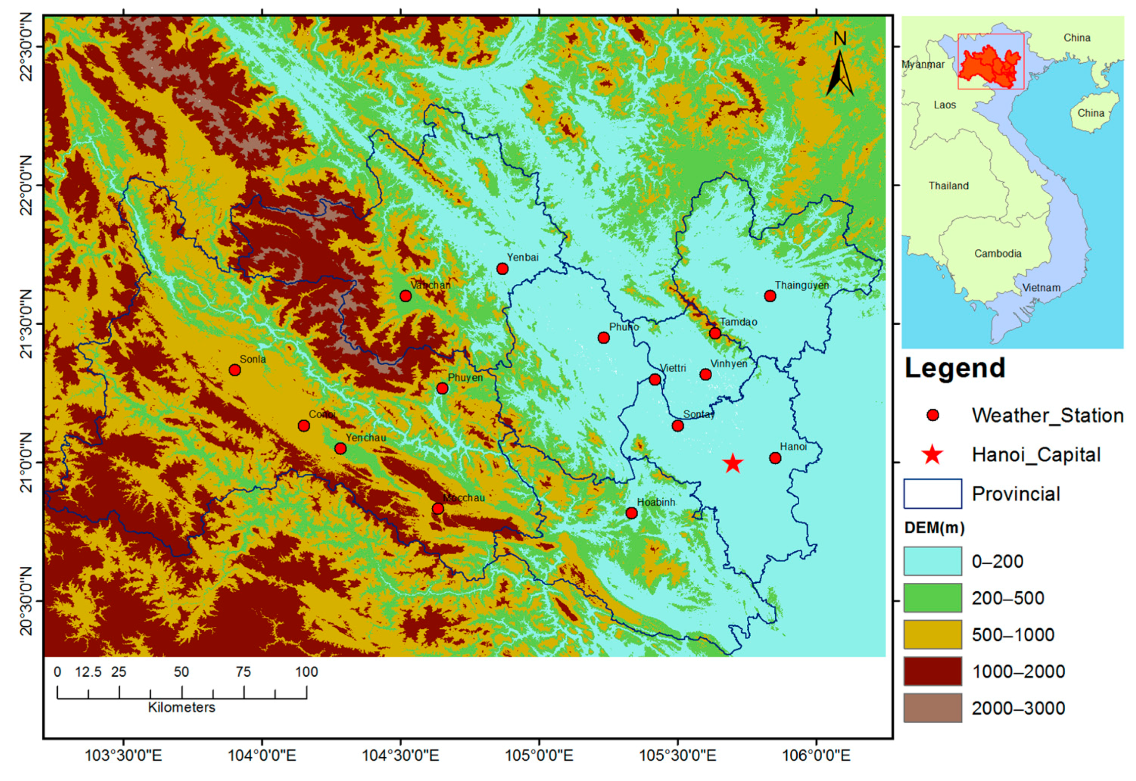
2.1. Study Area

The study area is located in northern Vietnam and covers more than 37,000 km², comprising the provinces of Hoa Binh, Ha Noi, Vinh Phuc, Thai Nguyen, Yen Bai, Phu Tho and Son La (see Figure 1). The study area extends from 20°18′N–22°40′N and from 103°12′E–106°18′E. The elevation ranges from sea level to over 3000 m.

The northern Vietnam study site was chosen for the following reasons:

(1)

Good distribution of meteorological station network in comparison to southern Vietnam.

(2)

Wide range of elevation (from approximately sea level to more than 3000 m).

(3)

The spatial heterogeneity of land cover.

(4)

There is no study about T_a estimation using all 4 MODIS LST datasets in northern Vietnam.

In this area, the topography is quite complex, increasing from southeast to northwest, and mostly divided into two regions: lowland and highland. The low part includes: Hoabinh, Hanoi, Phutho, Vinhphuc and Thainguyen provinces. The high part includes 2 large provinces: a part of Yenbai and Sonla.

The climate and weather in this area also vary depending on the elevation and type of landscape. The humidity is high, with the average ranging around 84% a year.

In late October and early November 2008, there was torrential rain in northern and central Vietnam that triggered severe floods in this region [49].

The location and elevation of meteorological stations are shown in

Table 2. Geographical description of weather stations used in this study.

Weather Station	Latitude (°)	Longitude (°)	Elevation (m)
Conoi	21.13	104.15	671
Hanoi	21.02	105.80	6
Hoabinh	20.82	105.33	23
Mocchau	20.83	104.68	972
Phuho	21.45	105.23	54
Phuyen	21.27	104.63	169
Sonla	21.33	103.90	675
Sontay	21.13	105.50	16
Tamdao	21.47	105.65	934
Thainguyen	21.60	105.83	35
Vanchan	21.58	104.52	275
Viettri	21.30	105.42	30
Vinhyen	21.32	105.60	10
Yenbai	21.70	104.87	56
Yenchau	21.05	104.30	314

.

2.2. Data

2.2.1. Remote Sensing Data

MODIS LST Data

Two MODIS LST products (h27v06, Collection 5, from 2003–2013, over northern Vietnam) were used in this study: MOD11A1 daily land surface temperature and emissivity from the TERRA satellites and MYD11A1 daily land surface temperature and emissivity from the AQUA satellites. There exist 4 LST data records per day, two from the TERRA satellites and two others from the AQUA satellites, which pass over the study site (local solar time) mostly around 10:30 a.m., p.m. and 1:45 a.m. and p.m., respectively. These times are relatively close to the times of maximum and minimum T_a daily data. In total, there were more than 8000 images (in HDF format, from 1 January 2003–31 December 2013) downloaded from the U.S. Geological Survey [50]. The MODIS LST is generated using a split-window algorithm [51] with two thermal infrared bands, 31 (10.78–11.28 μm) and 32 (11.77–12.27 μm). These two products (MOD11A1 and MYD11A1) have been validated, and the accuracy was reported better than 1 K under clear sky conditions [52].

Elevation

In this study area, the elevation is quite complex; it ranges from sea level to above 3000 m (see Figure 1). Generally, higher elevations are associated with lower temperatures. Elevation data were obtained from ASTER Global DEM. This data are available from the U.S. Geological Survey (USGS) with a spatial resolution of 30 m. These elevation data were resized to 1-km resolution using the nearest neighbor resampling type in order to be associated with other data resolutions, such as MODIS LST or NDVI data.

Vegetation Based on NDVI

Several studies have shown that the vegetation cover on the surface can affect LST values [53]. Vegetation cover (NDVI) data are provided every 16 days at 1-kilometer spatial resolution from the MODIS satellite, including MOD13A2 (TERRA 16-days period starting Day 001) and MYD13A2 (AQUA 16-day period starting Day 009). There are some studies that use both MOD13A2 and MYD13A2 in order to composite 8-day period data by averaging these two products [18]. Miura and Yoshioka [54] stated that MOD13A2 and MYD13A2 could be interchangeable. We assumed that NDVI did not change within 16 days. Therefore, in this study, to correct the influence of vegetation, we used NDVI 16 days data at 1-km resolution obtained from the MOD13A2 product.

2.2.2. Meteorological Data

Daily maximum and minimum air temperature data have been collected from 15 meteorological stations in northern Vietnam (see Figure 1), from 2003–2013. The data were obtained from the Vietnam Institute of Meteorology, Hydrology and ENvironment (IMHEN).

2.2.3. Auxiliary Data

Day length (Dlth) is the total time that any portion of the Sun is above the horizon. Typically (for low and mid-latitude locations), this will be the elapsed time beginning at sunrise and ending at sunset [55]. In this study, the day length (in hours) was downloaded from the Astronomical Applications Department of the U.S. Naval Observatory website [55].

The Julian day (Jd) was extracted from NASA server [56]. Both Julian day and day length are proxies for the fraction of solar energy absorption during the day and emitted energy during the night, influencing the diurnal amplitude of T_a throughout the year. Jang et al. [57] showed that the Julian day was a more significant parameter than altitude or the solar zenith angle in the inter-seasonal estimation of T_a. In order to understand the effect of viewing angle in the temporal variations in LST, especially in rugged regions, the view zenith angle (VZA) of daytime and nighttime should be taken into consideration [58]. In this study, there are four types of VZA of TERRA daytime, TERRA nighttime, AQUA daytime, AQUA nighttime (VZA_td, VZA_tn, VZA_ad, VZA_an, respectively). These data were collected from MOD11A1 and MYD11A1 products. We also took the effects of the latitude, longitude and elevation of each station, collected from IMHEN, into consideration to estimate T_a accuracy. All key terms and their explanations are summarized in

Table 3. Description of the key terminology used in this study.

Used Terms	Description
Ta (°C)	Land air surface temperature
Ta-max (°C)	Daily Maximum Ta
Ta-min (°C)	Daily Minimum Ta
LST (°C)	Land surface temperature
LSTtd (°C)	TERRA LST daytime
LSTtn (°C)	TERRA LST nighttime
LSTad (°C)	AQUA LST daytime
LSTan (°C)	AQUA LST nighttime
Ta-min-es (°C)	Daily minimum Ta estimation
Ta-max-es (°C)	Daily maximum Ta estimation
Ele (m)	Elevation of weather stations
NDVI	Normalized Difference Vegetation Index
Long (°)	Longitude
Lat (°)	Latitude
Dlth (hours)	Day length in hours
Jd	Julian day
VZAtd	View zenith angle of TERRA daytime
VZAtn	View zenith angle of TERRA nighttime
VZAad	View zenith angle of AQUA daytime
VZAan	View zenith angle of AQUA nighttime

.

2.3. Preprocessing Data

There were 8036 files of MODIS HDF format (MOD11A1 and MYD11A1, Version 5) from 1 January 2003–31 December 2013 that were downloaded for this study. Because all MODIS data were downloaded from USGS in HDF format (Hierarchical Data Format), with each file containing 12 data layers [58], we used the MODIS Reprojection Tool to extract the corresponding bands (LST_Day_1km, LST_Night_1km and view zenith angle) from MOD11A1 and MYD11A1. Next, we used the layer stacking tool in Envi5.0 to stack images for time series analysis purposes, before clipping the images to fit to our study area using ArcGIS 10.1.

2.4. LST Data Retrieval at Weather Stations

LST data under clear sky conditions at weather stations were retrieved by the following steps:

(1) MODIS LST day and night was extracted from MOD11A1 and MYD11A1 data for the pixel in which the meteorological stations are located. It should be noted that in the MODIS LST (v005) product, LST values derived from a single clear-sky MODIS observation are selected from MOD11_L2 files if the viewing zenith angles are small or larger zenith angles have LST errors smaller than 2 K [58]. This means that MOD11A1 and MYD11A1 LST were not produced for pixels that are classed as cloudy or cloud contamination remaining.

(2) However, [58] also noted that pixels that are lightly or modestly cloud contaminated are not removed by using cloud-removing masks if the contamination is smaller than the normal temporal variations in clear-sky LST. Typically, these are thin and subpixel clouds that are difficult to detect by the algorithm. In this case, we applied two steps to remove those types of errors. First, we simply filter and remove all unrealistic LST data that had values greater than 100 °C and below −50 °C. Second, we calculated the difference between T_a-max versus LST daytime and T_a-min versus LST nighttime. Then, we applied a statistic outlier removal based on these differences’ histograms to detect and remove data with unusually large differences.

(3) All valid LST day and nighttime data of TERRA and AQUA were statistical compared with T_a-max and T_a-min, respectively.

2.5. Estimation of Land Air Surface Temperature Using MODIS LST and Auxiliary Data

The method for this study was based on a multivariate linear regression analysis. This method was chosen because it could be applied for sparse meteorological station networks like northern Vietnam. Although some interpolation methods may give a higher accuracy result, they are not possible for regions with poorly-distributed station networks [59]; or physical models [41] that require an unreliable amount of input data.

2.5.1. Variable Selection

Zaksek and Schroedter-Homscheidt [34] stated that T_a is driven more by LST than by direct solar radiation, meaning that LST is the most important variable for T_a estimation; in reference to previous studies [15,29,31,42,57], also in consideration of all of the available data that potentially have an effect on the accuracy of T_a estimation of the study area. We have collected 14 variables, including: LST products (4 variables), NDVI, elevation (DEM), latitude, longitude, day length in hours and Julian day, and 4 variables of the view zenith angle as the potential variables (candidate variables) for T_a estimation.

Besides the 4 LST variables, we chose NDVI because it influences the land surface vegetation properties. Elevation, latitude and longitude were chosen for capturing the variability of climatic conditions between different regions. Day length in hours was chosen because we considered that it would affect the received solar radiation. Following [45,57], we chose Julian day because it reflects seasonal variation in air temperature. The view zenith angle was considered as a factor affecting the accuracy of LST data.

Since we have 14 potential variables (predictors), there are 2¹⁴ (= 16,384) possible models that could be applied for T_a-max and T_a-min estimation. Clearly, we cannot apply all of these possible models and test them one by one. Consequently, to save the time of data processing and to find the smallest model that best fits the data, we selected the best subset of variables among the 14 available variables.

In this study, we used several popular methods for variable selection, such as: (1) the Pearson correlation coefficient; (2) stepwise; (3) Bayesian information criterion (BIC); (4) adjusted R-squared; and (5) principal component analysis (PCA).

Pearson Correlation Coefficient

To select the variables for the multivariate linear regression models, we calculated the Pearson’s correlation coefficient (r) of all related variables. According to [11], r close to ±1 indicates a strong correlation; r = 0 means that there is no correlation; 0.25 ≤ r ≤ 0.75, means there is a moderate degree of correlation and 0 ≤ r < 0.25, a weak correlation. Based on this, we took only variables with r greater than 0.25 for T_a estimation.

The results in

Table 4. Pearson correlation coefficients of all variables considered in models for daily T_a-max and T_a-min estimation.

	LSTtd	LSTtn	LSTad	LSTan	NDVI	Ele	Long	Lat	Dlth	Jd	VZAtd	VZAtn	VZAad	VZAan
Ta-min	0.68	0.92	0.61	0.92	0.03	−0.29	0.27	−0.01	0.75	−0.17	0.00	0.01	−0.03	−0.01
Ta-max	0.85	0.86	0.86	0.82	−0.18	−0.28	−0.10	−0.08	0.68	−0.36	−0.01	0.03	−0.03	−0.03

All variables are described in Table 3.

show that we should use 7 variables for T_a-min estimated models (4 LST, Ele, Long and Dlth); and 7 other variables for T_a-max estimated models (4 LST, Ele, Dlth and Jd).

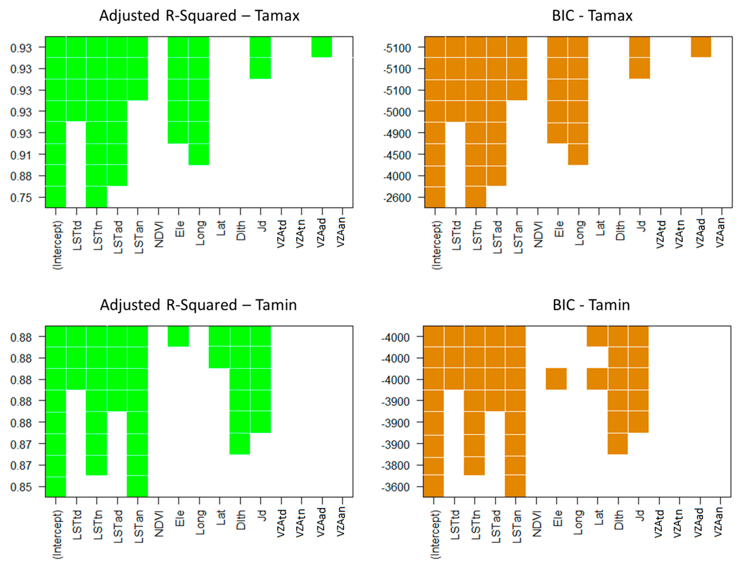
Variable Selection Based on Adjusted R-Squared (${\overline{\mathrm{R}}}^2$) and BIC

$${\overline{\mathrm{R}}}^2=1-\left(1-{\mathrm{r}}^2\right)\frac{\mathrm{N}-1}{\mathrm{N}-\mathrm{k}-1},$$

(1)

The best model will be the one with the largest value of ${\overline{\mathrm{R}}}^2$:

$$\mathrm{BIC}=\mathrm{Nlog}\left(\frac{\mathrm{SSE}}{\mathrm{N}}\right)+\left(\mathrm{k}+2\right)\log \left(\mathrm{N}\right),$$

(2)

Minimizing the BIC is intended to give the best model.

N is the number of observations; k is the number of predictors (variables); r² is the coefficient of determination; and SSE is the sum of squared error.

In Figure 2, colored parts (green for ${\overline{\mathrm{R}}}^2$ and orange for BIC) indicate that a variable was included in the model and white color that a variable was not included in the model. All of these models include the intercept.

Looking at the y-axis of Figure 2, it can be clearly seen that, in both cases of T_a-max and T_a-min, the top three models have the same results of ${\overline{\mathrm{R}}}^2$ and BIC.

In this case, we chose all top 3 models for T_a estimation. These model forms are as follows:

T_a-max = a × LST_td + b × LST_tn + c × LST_ad + d × LST_an +e × Ele +f × Long + g × Jd + h × VZAad + i,

(3)

T_a-max = a × LST_td + b × LST_tn + c × LST_ad + d × LST_an + e × Ele + f × Long + g × Jd + h,

(4)

T_a-max = a × LST_td + b × LST_tn + c × LST_ad + d × LST_an + e × Ele + f × Long + g,

(5)

T_a-min = a × LST_td + b × LST_tn + c × LST_ad + d × LST_an + e × Dlth + f × Lat + g × Jd +h × Ele + i,

(6)

T_a-min = a × LST_td + b × LST_tn + c × LST_ad + d × LST_an + e × Dlth + f × Lat + g × Jd + h,

(7)

T_a-min = a × LST_td + b × LST_tn + c × LST_ad + d × LST_an + e × Dlth + f × Jd + g.

(8)

Variable Selection Using Forward, Backward and Stepwise

Another popular method that is used for variable selection is the stepwise method. In this method, there are three types of operative steps: forward, backward and stepwise.

Forward selection starts with no variable in the model (intercept only model). In the next steps, the most significant variables are added to the model one by one. The process stops when all of the variables not in the model have a p-value greater than 0.15.

Backward elimination starts with the model including all variables. In the next step, the least significant variable will be removed. The procedure continues until all of the variables in the model have p-values less than or equal to 0.15.

The stepwise method adds or removes a variable in each step, depending on its p-value. This process continues until all variables within the model have a p-value ≤0.15, and all of the variables that were not in the model have a p-value >0.15.

Based on the results of forward, backward and stepwise selection, the T_a-max estimated model should include 12 variables (using all variables except VZA_tn and VZA_an); the T_a-min estimated model should include 10 variables (except long, VZA_an, VZA_td, VZA_tn).

The T_a-max and T_a-min estimated models were as follows:

T_a-max = a × LST_td + b × LST_tn + c × LST_ad + d × LST_an + e × NDVI + f × Ele + g × Long + h × Lat + i × Dlth + j × Jd + k × VZA_td + l × VZA_ad + m,

(9)

T_a-min = a × LST_td + b × LST_tn + c × LST_ad + d × LST_an + e × NDVI + f × Ele + g × Lat + h × Dlth + i × Jd + j × VZA_ad + k,

(10)

Variable Selection-Based Principal Component Analysis (PCA)

The result of the PCA showed that both T_a-max and T_a-min estimation models should include 4 LST, elevation, day length in hours and Julian day.

T_a-max = T_a-min = a × LST_td + b × LST_tn + c × LST_ad + d × LST_an +e × Ele +f × Dlth + g × Jd + h,

(11)

From all of the analyses above (Pearson correlation, ${\overline{\mathrm{R}}}^2$, BIC, stepwise and PCA), it is indicated that 4 LSTs (LST_td, LST_tn, LST_ad, LST_an) play an important role in T_a-max and T_a-min estimation, because they are always included in the top models of all above-mentioned methods.

To identify which LST data (LST_td, LST_tn, LST_ad, LST_an) are the best variables for T_a-max and T_a-min estimation, we have tested the ${\overline{\mathrm{R}}}^2$, BIC and stepwise analysis within 4 LST product. These results gave us 4 models (Models 1–4 for T_a-max, Models 10–13 for T_a-min estimation) in

Table 5. Model equations for T_a-max (1–9) and T_a-min (10–18) estimations.

	Models for Ta–max Estimations (*)		Models for Ta–min Estimations
1	Ta-max = a × LSTtn + b	10	Ta-min = a × LSTan + b
2	Ta-max = a × LSTtn + b × LSTad + c	11	Ta-min = a × LSTtn + b × LSTan + c
3	Ta-max = a × LSTtd + b × LSTtn + c × LSTad + d	12	Ta-min = a × LSTtn + b × LSTad + c × LSTan + d
4	Ta-max = a × LSTtd + b × LSTtn + c × LSTad + d × LSTan + e	13	Ta-min = a × LSTtd + b × LSTtn + c × LSTad + d × LSTan + e
5	Ta-max = a × LSTtd + b × LSTtn + c × LSTad + d × LSTan + e × Ele + f × Long + g	14	Ta-min = a × LSTtd + b × LSTtn + c × LSTad + d × LSTan + e × Dlth + f × Jd + g
6	Ta-max = a × LSTtd + b × LSTtn + c × LSTad + d × LSTan + e × Ele + f × Long + g × Jd + h	15	Ta-min = a × LSTtd + b × LSTtn + c × LSTad + d × LSTan + e × Dlth + f × Jd + g × Lat + h
7	Ta-max = a × LSTtd + b × LSTtn + c × LSTad + d × LSTan + e × Ele + f × Long + g × Jd+ h × VZAad + i	16	Ta-min = a × LSTtd + b × LSTtn + c × LSTad + d × LSTan + e × Dlth + f × Jd + g × Lat + h × Ele + i
8	Ta-max = a × LSTtd + b × LSTtn +c × LSTad + d × LSTan + e × NDVI + f × Ele + g × Long + h × Lat + i × Dlth + j × Jd + k × VZAtd + l × VZAad + m	17	Ta-min = a × LSTtd + b × LSTtn + c × LSTad + d × LSTan + e × NDVI + f × Ele + g × Lat + h × Dlth + i × Jd + j × VZAad + k
9	Ta-max = a × LSTtd + b × LSTtn + c × LSTad + d × LSTan + e × Ele + f × Dlth + g × Jd + h	18	Ta-min = a × LSTtd + b × LSTtn + c × LSTad + d × LSTan + e × Ele + f × Dlth + g × Jd + h

(*): Models 1–4 and 10–13 were chosen based on analysis of 4 LST products only. Model 5–7 and 14–16 were chosen from the top 3 models of ${\overline{\mathrm{R}}}^2$ and BIC criteria. Models 8 and 17 were chosen based on stepwise analysis. Models 9 and 18 were chosen based on PCA analysis. Models 9 is also the model with all significant variables identified using Pearson correlation determination. Letters a–m are model parameters. All variables are described in Table 3.

.

From Equations (3), (4), (5), (9) and (11), we build Models 5–9 for T_a-max estimation; Models 14–18 of T_a-min estimation were built based on Equations (6–8), (10) and (11).

We evaluated the models using the coefficient of determination (r²), the root mean square error (RMSE) and the mean absolute error (MAE). Because RMSE is very sensitive to outliers, hence MAE was chosen as an additional measure of the model quality.

$$\mathrm{RMSE}=\sqrt{\frac{1}{\mathrm{n}}{\sum }_{\mathrm{i}=1}^{\mathrm{n}}{\left({\mathrm{T}}_{\mathrm{a},\mathrm{i}}-{\mathrm{T}}_{\mathrm{es},\mathrm{i}}\right)}^2},$$

(12)

$$\mathrm{MAE}=\frac{1}{\mathrm{n}}{\sum }_{\mathrm{i}=1}^{\mathrm{n}}\left|{\mathrm{T}}_{\mathrm{a},\mathrm{i}}-{\mathrm{T}}_{\mathrm{es},\mathrm{i}}\right|$$

(13)

where T_a,i is the observed land air surface temperature from weather stations and T_es,i is the corresponding land air surface temperature estimated using linear regression analysis methods.

2.5.2. Model Calibration and Validation

For calibration and validation purposes, all data were randomly divided into two parts: calibration and validation datasets using a 70%/30% proportion, respectively.

To calculate the model coefficients a–m (see Table 5) for the models, we applied a least squares fitting analysis to the calibration dataset. The constant coefficients are listed in Appendix A and Appendix B. To validate the models, we applied the constant coefficients, which were calculated based on the calibration dataset, to the validate dataset.

3. Results

3.1. The Relationship between MODIS LST and T_a

In order to analyze the relations between T_a and all MODIS LST data, we calculated the coefficient of determination (r²), root mean square error (RMSE) and mean absolute error (MAE) of each type of MODIS LST (TERRA daytime, TERRA nighttime, AQUA daytime and AQUA nighttime) solely with T_a measured from weather stations.

Figure 3a shows that LST nighttime of both TERRA and AQUA showed a stronger correlation with T_a (both T_a-max and T_a-min) than for LST daytime. This can be explained by the fact that during the night, solar radiation does not affect the thermal infrared signal. Looking at the overpasses time of the satellite, the overpass time of AQUA daytime (around 1:45 p.m.) is later than the overpass time of TERRA (10:30 a.m.), as more solar radiation had been received by the land surface. As a result, LST AQUA daytime is hotter than LST TERRA daytime. Similarly, the overpass time of TERRA LST nighttime is around 10.30 p.m., three hours earlier than that of AQUA (1.45 a.m.), and the LST nighttime of TERRA is slightly higher than that of AQUA. This could be reflected by the cooling process of the land’s surface at night.

It also showed that LST nighttime of TERRA seems to perform better than LST nighttime of AQUA for T_a-max estimation. In contrast, LST nighttime of AQUA seemed better than LST nighttime of TERRA for T_a-min estimation.

In order to analyze which of the four LST variables is the best suited T_a estimation, we used the adjusted R-squared and BIC criteria (Figure 3b). Among the resulting models, we chose the one that only contained one variable. This variable is as such the best to estimate T_a.

It can be clearly seen that, based on the adjusted R-squared and BIC criteria (Figure 3b), the LST nighttime of TERRA and of AQUA were the best variables for T_a-max and T_a-min estimation, respectively. This result was consistent with the result shown in Figure 3a.

This result also indicates that the overpass time of satellites and the time of T_a-max, T_a-min recorded had no key influence on the relationship between T_a and LST. This is consistent with other research [8,25].

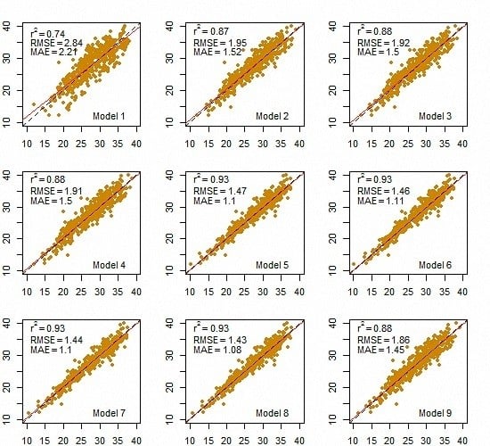
3.2. Ta-Max Estimation

The parameters of models for T_a-max estimation were determined when we applied Models 1–9 to the calibration dataset. This result is shown in Appendix A.

Figure 4 show that the results of the nine models were consistent with the processing in Section 2.5. Model 1 showed the lowest result, followed by Models 2–4.

Models 5–8 presented similar high results. However, Model 5 used only six variables; Models 6, 7 and 8 used 7, 8 and 12 variables, respectively. Based on this point, Model 5 would be chosen as the best model of T_a-max estimation.

Combining LST TERRA nighttime and LST AQUA daytime (Model 2), the result of T_a-max estimation was significantly better than Model 1 using LST TERRA nighttime solely. However, when we added LST TERRA daytime (Model 3, three variables), LST TERRA daytime and LST AQUA nighttime (Model 4, four variables), the performance of these models was not significantly improved in comparison to Model 2 (using two variables).

Comparing Model 4 and Model 5, it can be seen that, by combining four LSTs and elevation (Ele), longitude (Long) into the model, the result was much higher than using four LSTs only. This indicates that elevation (Ele), as well as the location (Long) of the weather station play an important role in T_a-max estimation.

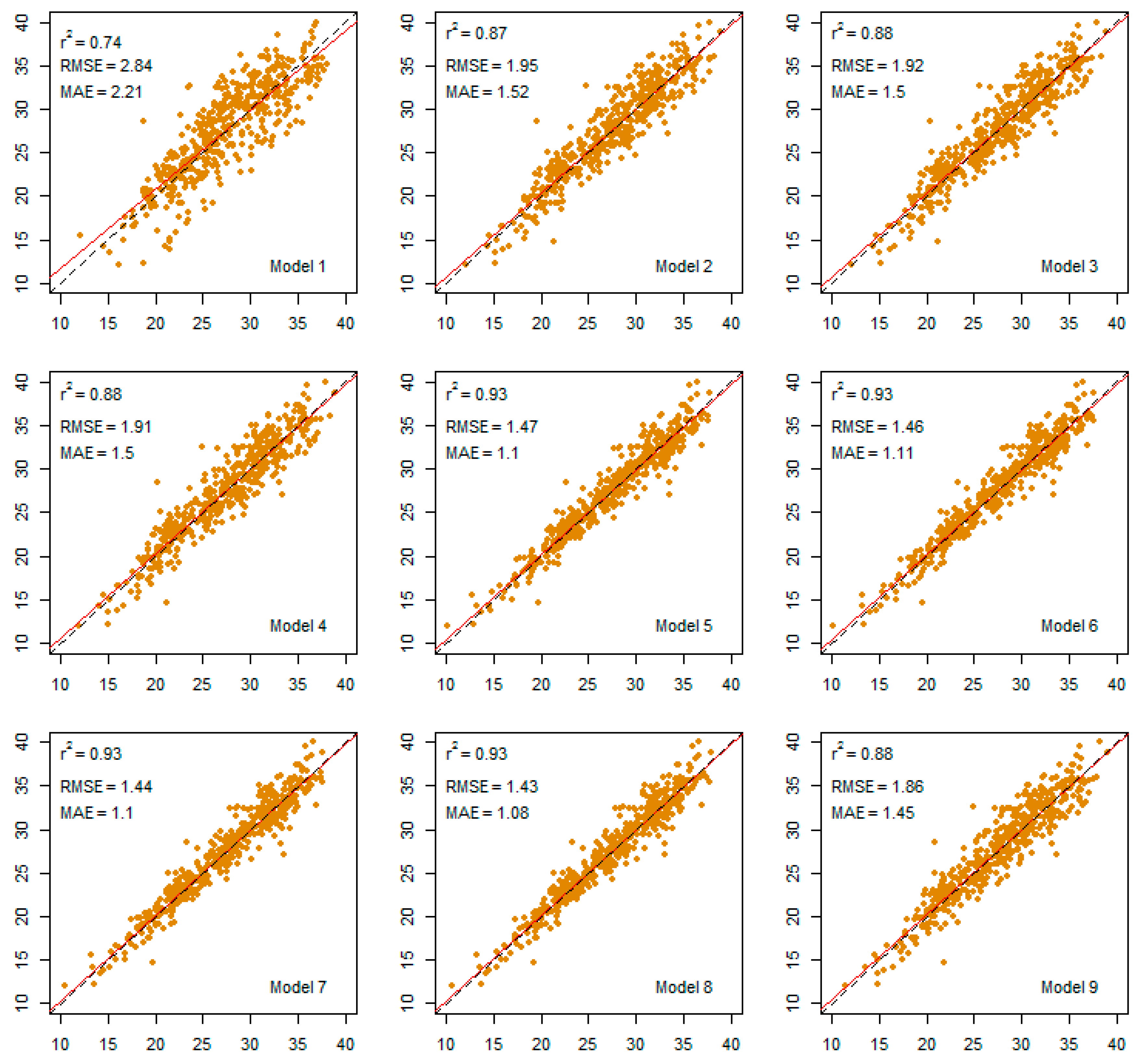
3.3. Ta-Min Estimation

The parameters of models for T_a-min estimation were determined when we applied Models 10–18 to the calibration dataset. This result is shown in Appendix B.

In general, Figure 5 shows that all models gave similar results of T_a-min estimation. From the simple model with two variables to the complex model (Model 17) using 10 variables, the results are similar. Figure 5 also shows that T_a-min estimation can reach a very high accuracy (r² = 0.85, RMSE = 2.31, MAE = 1.75) when using only one variable: LST_an. However, it was difficult to increase the accuracy of T_a-min estimated even with 10 variables or all 14 variables (see Figure 5).

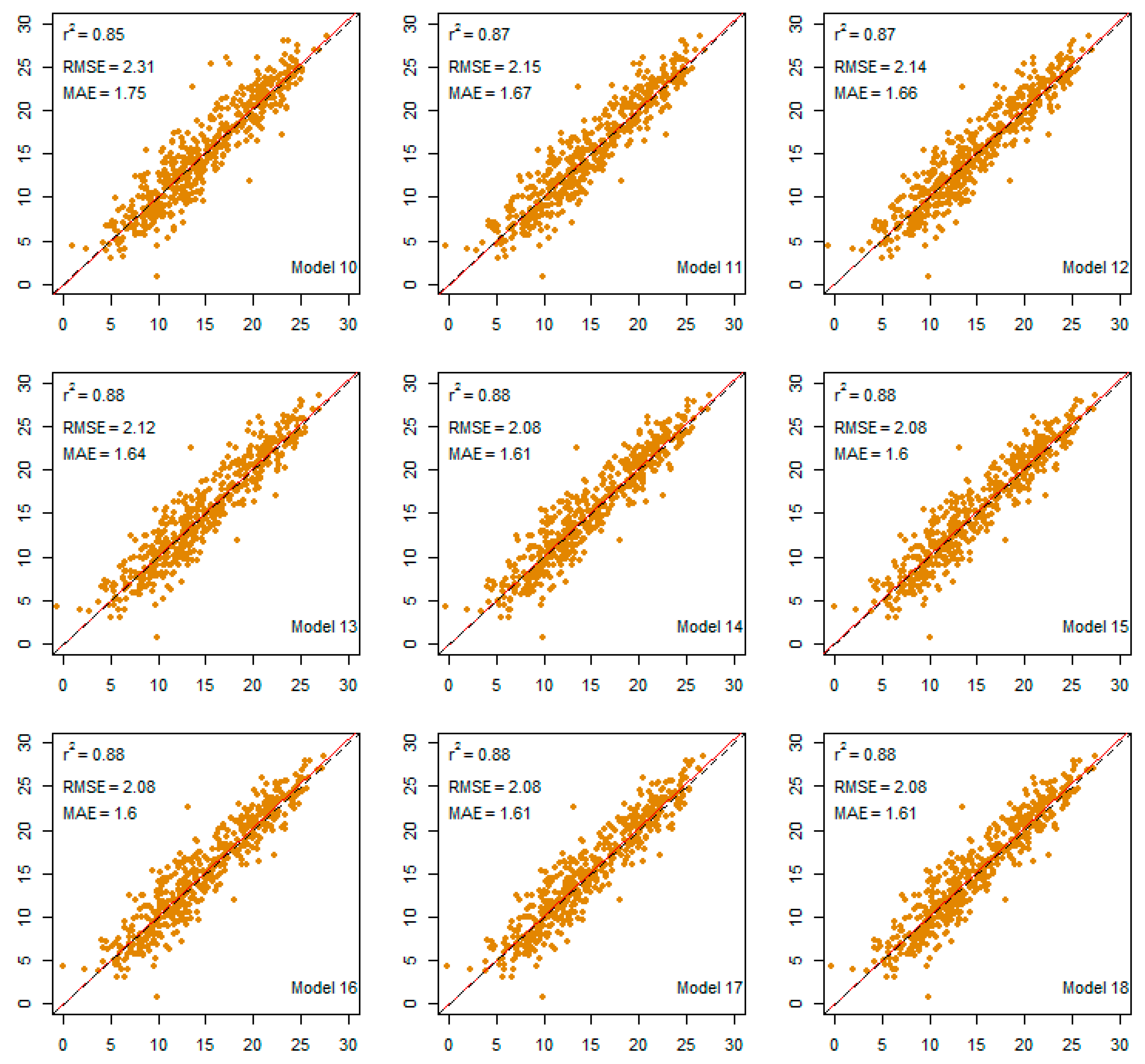
3.4. Performance of the Best Model

In order to test the effect of weather station location, as well as the seasonal change or any other factor related to station characteristics, we applied the best model to all datasets. The results are shown in Figure 6.

Looking at Figure 4, Figure 5 and Figure 6, it can be clearly seen that there are similar results of Model 5 and Model 15 when we applied them to the validation dataset or to all datasets. This consistent result indicates that there is no significant factor that could affect the accuracy of T_a estimation when Model 5 and Model 15 were applied for T_a-max and T_a-min estimation, respectively.

4. Discussion

4.1. MODIS LST Products for T_a Estimation

There are two MODIS sensors, TERRA and AQUA, which provides LST data four times daily (i.e., LST_td, LST_tn, LST_ad, LST_an). Most previous studies have used LST daytime for T_a-max and LST nighttime for T_a-min estimation. Some studies used only TERRA MODIS LST for T_a estimation [45,46]. There is a handful studies using LST daytime for T_a-min and LST nighttime for T_a-max estimation [29,42].

As far as we know, there have also been several studies using both LST daytime and nighttime of both MODIS sensors on TERRA and AQUA for their T_a estimated models [15,33,42,60]. However, the purpose of using four times daily LST was for filling the missing LST value. In our study, it is required that all four LST data have to be available.

Zhang et al. [42] combine TERRA LST daytime and nighttime (two variables), AQUA LST daytime and nighttime (also two variables) for T_a estimation and concluded that: (i) nighttime LST was better than daytime for deriving daily T_a; and (ii) incorporating daytime and nighttime LST significantly improved the estimation of T_a, as compared to using LST nighttime or daytime solely. Our results were consistent with this study [42]; however, our analysis could provide an even deeper insight into the matter. Model 2 and Figure 3b show that the combination of TERRA LST nighttime and AQUA LST daytime is even better than that of TERRA LST daytime and TERRA LST nighttime.

For T_a-max estimation, Figure 4 shows that if only LST products are used (without auxiliary data) the best result was achieved when we combined all four LST data (model 4). However, the Model 4 result (using four LSTs) was just slightly better than Model 2 (using only LST_tn and LST_ad).

Similarly, the best result of T_a-min estimation was achieved when we combined all four LSTs (Model 13). The combination of LST_tn and LST_an (Model 11) made the result of T_a-min estimation better than using LST_an solely (Model 10).

As we can see from Figure 2, T_a-min has a stronger correlation with LST nighttime of both TERRA and AQUA than T_a-max. However, as the final result, T_a estimation and T_a-max estimation show a much higher accuracy than T_a-min.

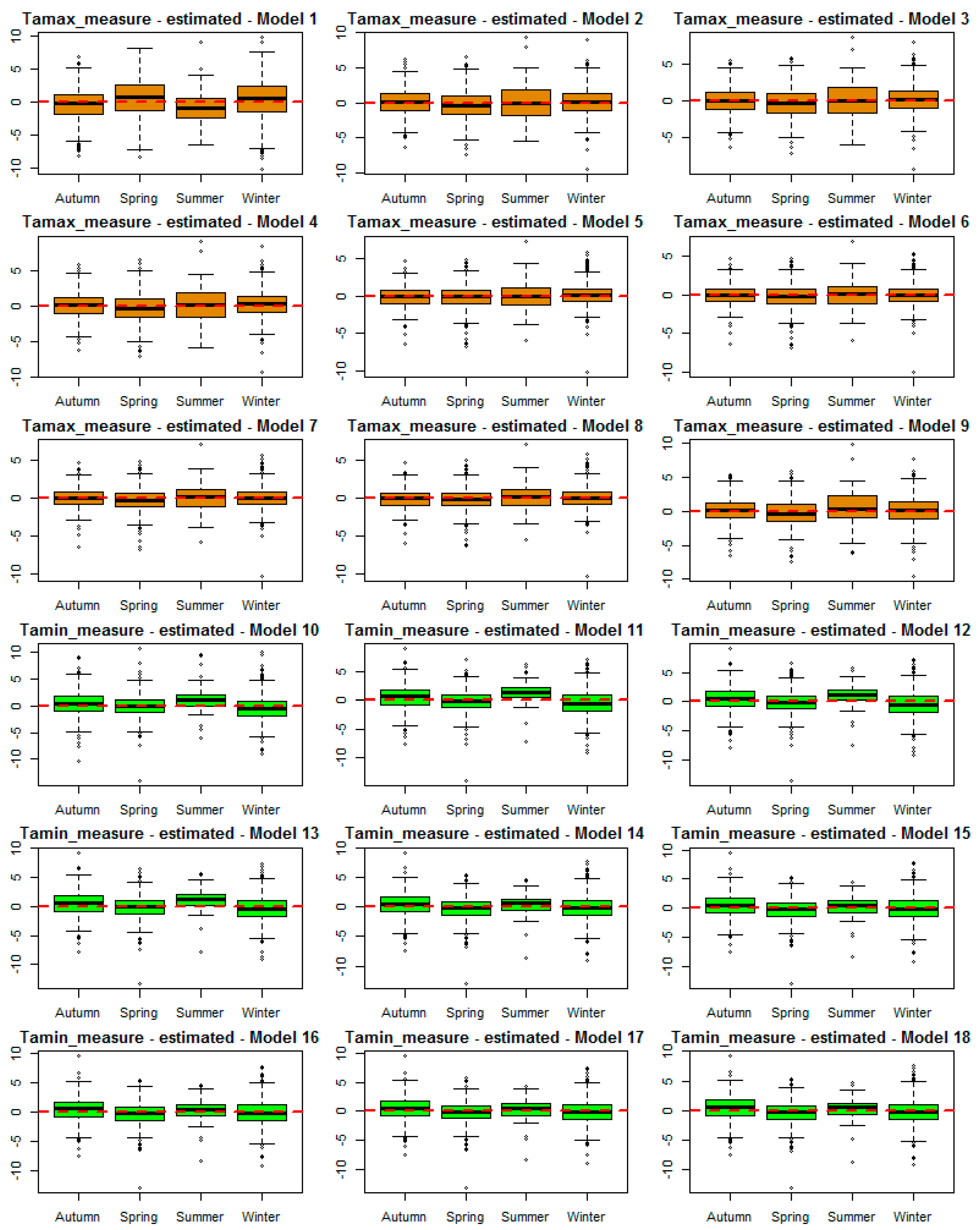
4.2. Effect of Seasonal on the Accuracy of T_a Estimation

To examine the effect of seasons on the relationship between LST and T_a (T_a-max and T_a-min), we separated the data into four seasons: spring (March, April, May), summer (June, July, August), autumn (September, October, November) and winter (December, January, February).

Looking at the nine upper panels (T_a-max estimation) of Figure 7, it can be seen that the accuracy of T_a-max estimation was significantly improved through different models. Models 1, 2, 3 and 4 show a low accuracy of T_a-max estimated in summer. Models 5, 6, 7 and 8 show a similar accuracy of T_a-max estimation. Model 9 again shows a low accuracy in summer. This means that, if we estimate T_a-max using LST data without other auxiliary data, the results would not be accurate. This can be explained by, as in the summer, the land surface receiving more solar radiation, and as such, the relation between T_a and LST becomes more complex.

In general, the changing season had no significant effect on the accuracy of T_a estimation if we use all four LST data and other variables for linear regression.

4.3. Effect of View Zenith Angle on the Accuracy of T_a Estimation

As mentioned in Section 2.4, LST data were collected at smaller viewing zenith angles or LST retrievals at larger zenith angles, but with LST errors smaller than at least 2 K.

In order to check the effect of VZA on the relationship between MODIS LST and T_a, we divided the data into three groups based on the range of VZA: bl40 (0° ≤ VZA ≤ 40°), f41t90 (41° ≤ VZA ≤ 90°) and f91t130 (91° ≤ VZA ≤ 130°). Using all linear regression models in Table 5 for T_a-max and T_a-min estimation, we then calculated the difference between T_a estimated and T_a measured (difference = T_a measured − T_a estimated). These differences are shown in Figure 8. Although the differences might vary from Models 1–9 of T_a-max estimation and Models 10–18 of T_a-min estimation, it was similar between the three groups through all models. This indicates that the effect of VZA on the result of T_a estimation was not significant.

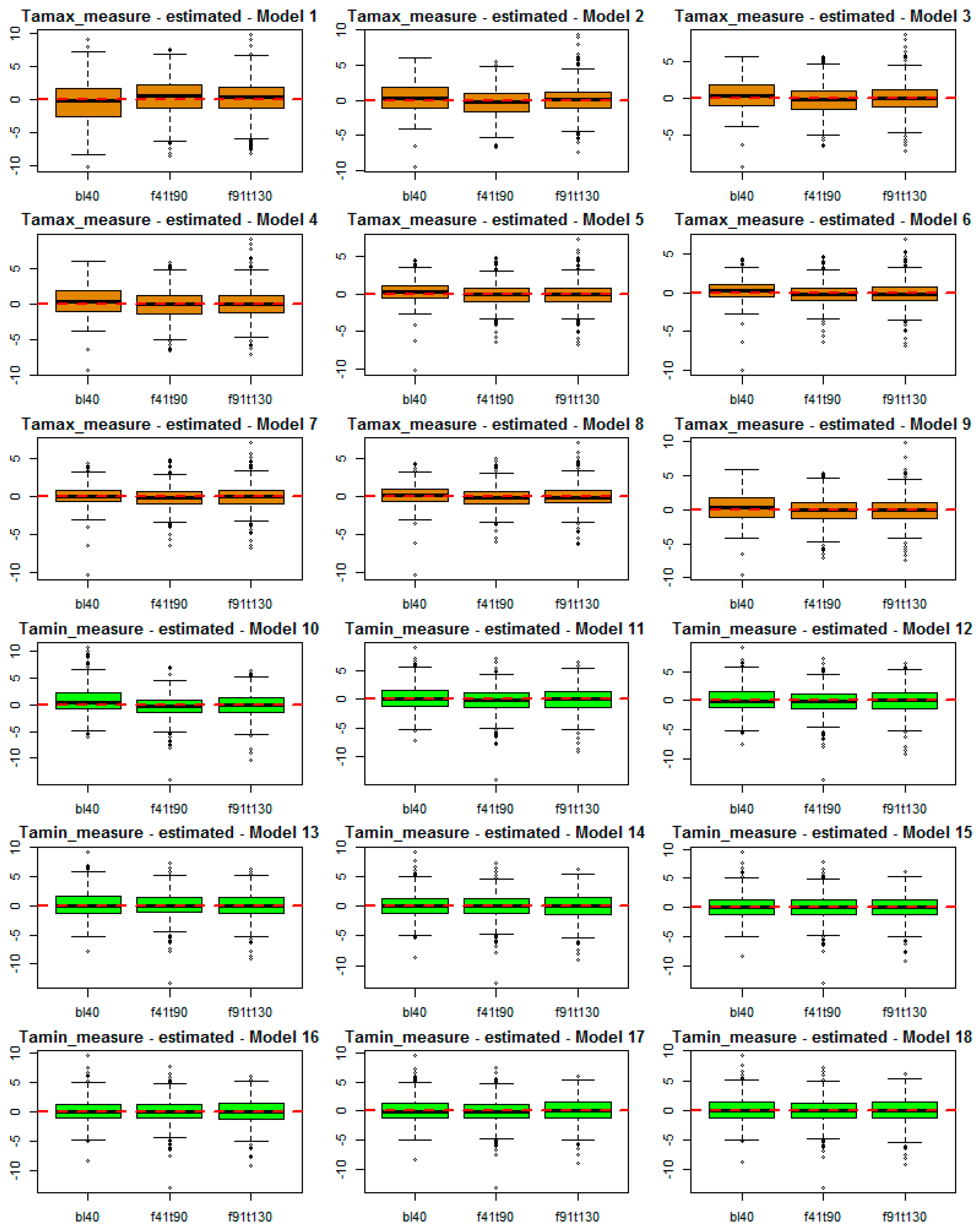
4.4. Effect of Station Elevation on Accuracy

To test the effect of weather station elevation on the estimation results, we divided the data into three regions: bl200m, f200t500m and ov500m. The bl200m region includes stations that have an elevation below 200 m; the f200t500m region includes stations having an elevation from 200–500 m; and ov500m region includes stations that have an elevation higher than 500 m. It should be noted that this division is just one option to test the effect of station altitude that might affect the results. It could be divided into more parts for more detail (the more parts are divided, the more detail on the differences could be achieved). We calculated the difference between T_a estimated and T_a measured of these three groups of elevation (difference = T_a measured − T_a estimated). These differences are shown in Figure 9.

As we can see in Figure 9, for T_a-max, the differences of three groups were variations from Models 1–9. The most significant was found in Model 1 and Model 9. Models 5, 6, 7 and 8 showed a similar difference between three groups. This indicates that we can reduce the effect of the station‘s elevation by using Model 5, 6, 7 or 8.

Looking at Table 5, we found that all of Models 5, 6, 7 and 8 include longitude and elevation variable in the models. Model 9 also has the elevation variable in it, but Figure 9 shows that there is a difference between the three elevation groups. It could be concluded that the longitude variable affects the T_a-max estimation.

Regarding T_a-min estimation, Figure 9 shows a similar result of all models (from Models 10–18) and a similar performance between the three elevation groups. This indicates that the station’s elevation has no effect on T_a-min estimation.

4.5. Accuracy Improvement by Integrating Four LST Products and Auxiliary Variables

4.5.1. For T_a-max Estimation

When comparing the results of Model 4 (using four LST data) versus Models 5–9 (using four LST data and auxiliary data; see Figure 4), it can be clearly seen that the results were significantly improved. The coefficient of determination (r²) was increased from 0.88–0.93; RMSE and MAE were decreased from 1.91 down to 1.43 and 1.50 down to 1.08 °C respectively.

The performances of Models 5, 6 and 7 were similar and had very high accuracy. As shown in the variable selection section (Section 2.5.1), these models came from the top three models of adjusted R-squared and BIC criteria.

Model 8, which was chosen from stepwise regression, showed a similar result of accuracy. However, this model used up to 12 variables.

Model 9, which was chosen based on PCA analysis, also showed a high accuracy result with r² = 0.88, RMSE = 1.86, and MAE = 1.45; however, this result was not as high as the results of Models 5, 6, 7, and 8.

Looking at Table 5, it can be clearly seen that Models 5–8 always include elevation and longitude variables. It would be expected that because Model 9 did not use the longitude variable, therefore the accuracy was not as good as Models 5, 6, 7 and 8.

This indicates that elevation and longitude are the most important variables for T_a-max estimation. This result is consistent with adjusted R-squared, BIC criteria and stepwise analysis.

4.5.2. For T_a-min Estimation

Looking at Figure 5, it can be clearly seen that the results of all nine models (Models 10–18) were not significantly different. In other words, the accuracy of the model was not increased from the simplest (Model 10, using one variable) to the most complex model (Model 17 with 10 variables).

In comparison to previous studies (see Table 1), we achieved better results (similar r², but smaller RMSE and MAE) of T_a-max estimation due to the combination of four LST data and auxiliary variables. However, this combination just made a slight improvement for the T_a-min estimation (comparing the result of Model 10, versus Models 11–18). In a further study, a better method for increasing the accuracy of T_a-min estimation should be examined.

Considering the coefficient of determination (r²), the accuracy (RMSE, MAE) and the number of variables used per model, we would regard Model 5 (for T_a-max estimation) and Model 15 (for T_a-min estimation) as the best models.

5. Conclusions

In this study, we have analyzed and discussed the relationship between T_a-max, T_a-min and four LST products (LST_td, LST_tn, LST_ad, LST_an). The simple method of multiple linear regression analysis was used, and a high accuracy was achieved with r² = 0.93, RMSE = 1.43, MAE = 1.08 and r² = 0.88, RMSE = 2.08, MAE = 1.60, for T_a-max and T_a-min, respectively.

When estimating T_a using one LST datum solely, T_a-min showed a better result than T_a-max (Model 1 versus Model 10 in Figure 4 and Figure 5). Multiple linear regressions always give better results than simple linear.

An interesting result is that when we directly compared LST data versus T_a, LST nighttime showed a stronger correlation with both T_a-max and T_a-min than LST daytime; T_a-min had a better correlation with LST data than T_a-max (see Figure 3a). However, the results of modeling showed that T_a-max can be estimated with better results (higher r² and lower RMSE, MAE) than T_a-min when adding auxiliary variables into the models. It could be concluded that in T_a estimation, it is not possible to see the relationship between T_a and LST from a directed comparison, because there are other factors that also affect that relationship.

Several model analyses indicate that MODIS LST represents the most important variables for T_a estimation. However, to achieve the best results, other variables, such as day length (in hours), Julian day, longitude, latitude and elevation, should be taken into consideration and put into the models.

References

1. De Bruin, H.A.R.; Trigo, I.F.; Jitan, M.A.; TemesgenEnku, N.; van der Tol, C.; Gieske, A.S.M. Reference crop evapotranspiration derived from geo-stationary satellite imagery: A case study for the Fogera flood plain, NW-Ethiopia and the Jordan Valley, Jordan. Hydrol. Earth Syst. Sci. 2010, 14, 2219–2228. [Google Scholar] [CrossRef]
2. Balaghi, R.; Tychon, B.; Eerens, H.; Jlibene, M. Empirical regression models using NDVI, rainfall and temperature data for early prediction of wheat grain yields in Morocco. Int. J. Appl. Earth Obs. 2008, 10, 438–452. [Google Scholar] [CrossRef]
3. De Wit, A.J.W.; van Diepen, C.A. Crop growth modelling and crop yield forecasting using satellite-derived meteorological inputs. Int. J. Appl. Earth Obs. 2008, 10, 414–425. [Google Scholar] [CrossRef]
4. Lehman, J.T. Application of satellite AVHRR to water balance mixing dynamics and the chemistry of Lake Edward, East Africa. In The East African Great Lakes: Limnology, Palaeolimnology and Biodiversity; Odada, E.O., Olago, D.O., Eds.; Kluwer Academic Publishers: Dordrecht, The Netherlands, 2002; pp. 235–260. [Google Scholar]
5. Vallet-Coulomb, C.; Legesse, D.; Gasse, F.; Travi, Y.; Chernet, T. Lake evaporation estimates in tropical Africa (Lake Ziway, Ethiopia). J. Hydrol. 2001, 245, 1–18. [Google Scholar] [CrossRef]
6. Intergovernmental Panel on Climate Change (IPCC). Climate Change 2001: The Scientific Basis; Contribution of Working Group I to the Third Assessment Report of the Intergovernmental Panel on Climate Change; Cambridge University Press: Cambridge, UK, 2001; p. 881. [Google Scholar]
7. Intergovernmental Panel on Climate Change (IPCC). Climate Change 2007: The Physical Science Basis; Contribution of Working Group I to the Fourth Assessment Report of the Intergovernmental Panel on Cli-mate Change; Solomon, S., Qin, D., Manning, M., Chen, Z., Marquis, M., Averyt, K.B., Tignor, M., Miller, H.L., Eds.; Cambridge University Press: Cambridge, UK, 2007. [Google Scholar]
8. Fu, G.; Shen, Z.X.; Zhang, X.Z.; Shi, P.L.; Zhang, Y.J.; Wu, J.S. Estimating air temperature of an alpine meadow on the Northern Tibetan Plateau using MODIS land surface temperature. Acta Ecol. Sin. 2011, 21, 8–13. [Google Scholar] [CrossRef]
9. Stisen, S.; Sandholt, I.; Norgaard, A.; Fensholt, R.; Eklundh, L. Estimation of diurnal air temperature using MSG SEVIRI data in West Africa. Remote Sens. Environ. 2007, 110, 262–274. [Google Scholar] [CrossRef]
10. Nieto, H.; Sandholt, I.; Aguado, I.; Chuvieco, E.; Stisen, S. Air temperature estimation with MSG-SEVIRI data: Calibration and validation of the TVX algorithm for the Iberian Peninsula. Remote Sens. Environ. 2011, 115, 107–116. [Google Scholar] [CrossRef]
11. Lin, S.; Moore, N.J.; Messina, J.P.; de Visser, M.H.; Wu, J. Evaluation of estimating daily maximum and minimum air temperature with MODIS data in east Africa. Int. J. Appl. Earth Obs. Geoinf. 2012, 18, 128–140. [Google Scholar] [CrossRef]
12. Basist, A.N.; Peterson, N.C.; Peterson, T.C.; Williams, C.N. Using the special sensor mi-crowave/imager to monitor land surface temperature, wetness, and snow cover. J. Appl. Meteorol. 1998, 37, 888–911. [Google Scholar] [CrossRef]
13. Peterson, T.C.; Basist, A.N.; Williams, C.; Grody, N. A blended satellite/in situ near-global surface temperature data set. Bull. Am. Meteorol. Soc. 2000, 81, 2157–2164. [Google Scholar] [CrossRef]
14. Florio, E.N.; Lele, S.R.; Chi Chang, Y.; Sterner, R.; Glass, G.E. Integrating AVHRR satellite data and NOAA ground observations to predict surface air temperature: A statistical approach. Int. J. Remote Sens. 2004, 25, 2979–2994. [Google Scholar] [CrossRef]
15. Vancutsem, C.; Ceccato, P.; Dinku, T.; Connor, S.J. Evaluation of MODIS land surface temperature data to estimate air temperature in different ecosystems over Africa. Remote Sens. Environ. 2010, 114, 449–465. [Google Scholar] [CrossRef]
16. Vogt, J.V.; Viau, A.A.; Paquet, F. Mapping regional air temperature fields using satellite-derived surface skin temperatures. Int. J. Climatol. 1997, 17, 1559–1579. [Google Scholar] [CrossRef]
17. Lai, Y.J.; Li, C.F.; Lin, P.H.; Wey, T.H.; Chang, C.S. Comparison of MODIS land surface temperature and ground-based observed air temperature in complex topography. Int. J. Remote Sens. 2012, 33, 7685–7702. [Google Scholar] [CrossRef]
18. Sun, H.; Chen, Y.; Gong, A.; Zhao, X.; Zhan, W.; Wang, M. Estimating mean air temperature using MODIS day and night land surface temperatures. Theor. Appl. Climatol. 2014, 118, 81–92. [Google Scholar] [CrossRef]
19. Dinh, V.V. Country Report the hydro meteorological service of Vietnam and its modernization plan. In Proceedings of the 5th Global Precipitation Measurement (GPM) International Planning Workshop, Tokyo, Japan, 7–9 November 2005.
20. Coll, C.; Caselles, V.; Sobrino, J.A.; Valor, E. On the atmospheric dependence of the split-window equation for land surface temperature. Int. J. Remote Sens. Environ. 1994, 27, 105–122. [Google Scholar] [CrossRef]
21. Wan, Z.; Dozier, J. A generalized split-window algorithm for retrieving land-surface temperature from space. IEEE Trans. Geosci. Remote Sens. 1996, 34, 892–905. [Google Scholar]
22. Cresswell, M.P.; Morse, A.P.; Thomson, M.C.; Connor, S.J. Estimating surface air temperatures, from Meteosat land surface temperatures, using an empirical solar zenith angle model. Int. J. Remote Sens. 1999, 20, 1125–1132. [Google Scholar] [CrossRef]
23. Williamson, S.; Hik, D.; Gamon, J.; Kavanaugh, J.; Flowers, G. Estimating temperature fields from MODIS land surface temperature and air temperature observations in a sub-arctic alpine environment. Remote Sens. 2014, 6, 946–963. [Google Scholar] [CrossRef]
24. Prince, S.D.; Goetz, S.J.; Dubayah, R.O.; Czajkowski, K.P.; Thawley, M. Inference of surface and air temperature, atmospheric precipitable water and vapor pressure deficit using advanced very high-resolution radiometer satellite observations: Comparison with field observations. J. Hydrol. 1998, 213, 230–249. [Google Scholar] [CrossRef]
25. Mostovoy, G.V.; King, R.L.; Reddy, K.R.; Kakani, V.G.; Filippova, M.G. Statistical estimation of daily maximum and minimum air temperatures from MODIS LST data over the state of Mississippi. GISci. Remote Sens. 2006, 43, 78–110. [Google Scholar] [CrossRef]
26. Jin, M.; Dickinson, R.E. Land surface skin temperature climatology: Benefitting from the strengths of satellite observations. Environ. Res. Lett. 2010, 5, 044004. [Google Scholar] [CrossRef]
27. Lin, X.; Zhang, W.; Huang, Y.; Sun, W.; Han, P.; Yu, L.; Sun, F. Empirical estimation of near-surface air temperature in China from MODIS LST data by considering physiographic features. Remote Sens. 2016, 8, 629. [Google Scholar] [CrossRef]
28. Gallo, K.; Hale, R.; Tarpley, D.; YU, Y. Evaluation of the relationship between air and land surface temperature under clear- and cloudy-sky conditions. J. Appl. Meteorol. Climatol. 2011, 50, 767–775. [Google Scholar] [CrossRef]
29. Benali, A.; Carvalho, A.C.; Nunes, J.P.; Carvalhais, N.; Santos, A. Estimating air surface temperature in Portugal using MODIS LST data. Remote Sens. Environ. 2012, 124, 108–121. [Google Scholar] [CrossRef]
30. Crosson, W.L.; Al-Hamdan, M.Z.; Hemmings, S.N.; Wade, G.M. A daily merged MODIS Aqua–Terra land surface temperature data set for the conterminous United States. Remote Sens. Environ. 2012, 119, 315–324. [Google Scholar] [CrossRef]
31. Zeng, L.; Wardlow, B.D.; Tadesse, T.; Shan, J.; Hayes, M.J.; Li, D.; Xiang, D. Estimation of daily air temperature based on MODIS land surface temperature products over the corn belt in the US. Remote Sens. 2015, 7, 951–970. [Google Scholar] [CrossRef]
32. Xu, Y.; Qin, Z.; Shen, Y. Study on the estimation of near-surface air temperature from MODIS data by statistical methods. Int. J. Remote Sens. 2012, 33, 7629–7643. [Google Scholar] [CrossRef]
33. Huang, R.; Zhang, C.; Huang, J.; Zhu, D.; Wang, L.; Liu, J. Mapping of daily mean air temperature in agricultural regions using daytime and nighttime land surface temperatures derived from Terra and Aqua MODIS data. Remote Sens. 2015, 7, 8728–8756. [Google Scholar] [CrossRef]
34. Zakšek, K.; Schroedter-Homscheidt, M. Parameterization of air temperature in high temporal and spatial resolution from a combination of the SEVIRI and MODIS instruments. ISPRS J. Photogramm. Remote Sens. 2009, 64, 414–421. [Google Scholar] [CrossRef]
35. Prihodko, L.; Goward, S.N. Estimation of air temperature from remotely sensed surface observations. Remote Sens. Environ. 1997, 60, 335–346. [Google Scholar] [CrossRef]
36. Goetz, S.J. Multi-sensor analysis of NDVI, surface temperature and biophysical variables at amixed grassland site. Int. J. Remote Sens. 1997, 18, 71–94. [Google Scholar] [CrossRef]
37. Goetz, S.J.; Prince, S.D.; Small, J. Advances in satellite remote sensing of environmental variables for epidemiological applications. Adv. Parasitol. 2000, 47, 289–307. [Google Scholar] [PubMed]
38. Zhu, W.; Lű, A.; Jia, S. Estimation of daily maximum and minimum air temperature using MODIS land surface temperature products. Remote Sens. Environ. 2013, 130, 62–73. [Google Scholar] [CrossRef]
39. Sun, H.; Zhao, X.; Chen, Y.; Gong, A.; Yang, J. A new agricultural drought monitoring index combining MODIS NDWI and day–night land surface temperatures: A case study in China. Int. J. Remote Sens. 2013, 34, 8986–9001. [Google Scholar] [CrossRef]
40. Sandholt, I.; Rasmussen, K.; Andersen, J. A simple interpretation of the surface temperature/vegetation index space for assessment of surface moisture status. Remote Sens. Environ. 2002, 79, 213–224. [Google Scholar] [CrossRef]
41. Sun, Y.J.; Wang, J.F.; Zhang, R.H.; Gillies, R.R.; Xue, Y.; Bo, Y.C. Air temperature retrieval from remote sensing data based on thermodynamics. Theor. Appl. Climatol. 2005, 80, 37–48. [Google Scholar] [CrossRef]
42. Zhang, W.; Huang, Y.; Yu, Y.; Sun, W. Empirical models for estimating daily maximum, minimum and mean air temperatures with MODIS land surface temperatures. Int. J. Remote Sens. 2011, 32, 9415–9440. [Google Scholar] [CrossRef]
43. Good, E. Daily minimum and maximum surface air temperatures from geostationary satellite data. J. Geophys. Res. Atmos. 2015, 120, 2306–2324. [Google Scholar] [CrossRef]
44. Zhang, R.; Rong, Y.; Tian, J.; Su, H.; Li, Z.L.; Liu, S. A remote sensing method for estimating surface air temperature and surface vapor pressure on a regional scale. Remote Sens. 2015, 7, 6005–6025. [Google Scholar] [CrossRef]
45. Janatian, N.; Sadeghi, M.; Sanaeinejad, S.H.; Bakhshian, E.; Farid, A.; Hasheminia, S.M.; Ghazanfari, S. A statistical framework for estimating air temperature using MODIS land surface temperature data. Int. J. Climatol. 2016. [Google Scholar] [CrossRef]
46. Shen, S.; Leptoukh, G.G. Estimation of surface air temperature over central and eastern Eurasia from MODIS land surface temperature. Environ. Res. Lett. 2011, 6, 045206. [Google Scholar] [CrossRef]
47. Emamifar, S.; Rahimikhoob, A.; Noroozi, A. Daily mean air temperature estimation from MODIS land surface temperature products based on M5 model tree. Int. J. Climatol. 2013, 33, 3174–3181. [Google Scholar] [CrossRef]
48. Xu, Y.; Knudby, A.; Ho, H.C. Estimating daily maximum air temperature from MODIS in British Columbia, Canada. Int. J. Remote Sens. 2014, 35, 8108–8121. [Google Scholar] [CrossRef]
49. NASA Visible Earth. Available online: http://visibleearth.nasa.gov/view.php?id=35791 (accessed on 12 October 2015).
50. The U.S. Geological Survey. MODIS LST Data. Available online: http://earthexplorer.usgs.gov (accessed on 1 August 2015).
51. Wan, Z.; Zhang, Y.; Zhang, Q.; Li, Z.L. Validation of the land-surface temperature products retrieved from Terra Moderate Resolution Imaging Spectroradiometer data. Remote Sens. Environ. 2002, 83, 163–180. [Google Scholar] [CrossRef]
52. The Report of MOD11A1 and MYD11A1 Validation Accuracy. Available online: http://landval.gsfc.nasa.gov/ProductStatus.php?ProductID=MOD11 (accessed on 2 November 2015).
53. Shi, L.; Liu, P.; Kloog, I.; Lee, M.; Kosheleva, A.; Schwartz, J. Estimating daily air temperature across the Southeastern United States using high-resolution satellite data: A statistical modeling study. Environ. Res. 2016, 146, 51–58. [Google Scholar] [CrossRef] [PubMed]
54. Miura, T.; Yoshioka, H.; Fujiwara, K.; Yamamoto, H. Inter-comparison of ASTER and MODIS surface reflectance and vegetation index products for synergistic applications to natural resource monitoring. Sensors 2008, 8, 2480–2499. [Google Scholar] [CrossRef] [PubMed]
55. The United States Naval Observatory (USNO). Day Length in Hours Data. Available online: http://aa.usno.navy.mil/data/docs/Dur_OneYear.php#formb (accessed on 1 December 2015).
56. Land Quality Assessment Site of NASA. Julian Day. Available online: http://landweb.nascom.nasa.gov/browse/calendar.html (accessed on 2 November 2015).
57. Jang, J.D.; Viau, A.A.; Anctil, F. Neural network estimation of air temperatures from AVHRR data. Int. J. Remote Sens. 2004, 25, 4541–4554. [Google Scholar] [CrossRef]
58. Wan, Z. MODIS Land Surface Temperature Products Users’ Guide. Available online: http://www.icess.ucsb.edu/modis/LstUsrGuide/MODIS_LST_products_Users_guide_C5.pdf (accessed on 19 November 2015).
59. Kilibarda, M.; Hengl, T.; Heuvelink, G.; Gräler, B.; Pebesma, E.; Perčec Tadić, M.; Bajat, B. Spatio-temporal interpolation of daily temperatures for global land areas at 1 km resolution. J. Geophys. Res. Atmos. 2014, 119, 2294–2313. [Google Scholar] [CrossRef]
60. Shamir, E.; Georgakakos, K.P. MODIS land surface temperature as an index of surface air temperature for operational snowpack estimation. Remote Sens. Environ. 2014, 152, 83–98. [Google Scholar] [CrossRef]
Figure 1. Location of the 15 meteorological stations in northern Vietnam and the range of elevations in the study area.
Remotesensing 08 01002 g001
Figure 2. Ranking of models based on R ¯ 2 and BIC criteria for Ta-max (upper row panel) and Ta-min (lower row panel) estimation.
Remotesensing 08 01002 g002
Figure 3. (a) The relationship between LST (x-axis) and Ta-max (upper panels), Ta-min (lower panels) of all meteorological stations from 2003–2013. The dashed green line indicates that the difference between Ta and LST is over +15 °C; the dashed blue line indicates that the difference between Ta and LST is lower than −15 °C. The dashed black line indicates the 1:1 line. The solid red line shows the regression line. (b) Adjusted R-squared and BIC criteria show the top four models of Ta-max (upper panel) and Ta-min (lower panel) estimation using only the four LST dataset.
Remotesensing 08 01002 g003
Figure 4. The relationship between Ta observed (y-axis) and Ta estimated (x-axis) using Models 1–9. The dashed black line indicates the 1:1 line. The solid red line shows the regression line.
Remotesensing 08 01002 g004
Figure 5. The relationship between Ta observed (y-axis) and Ta estimated (x-axis) using Models 10–18. The dashed black line indicates the 1:1 line. The solid red line shows the regression line.
Remotesensing 08 01002 g005
Figure 6. The comparison of estimated Ta using Model 5, Model 15 and the model using 14 variables. The dashed black line indicates the 1:1 line. The solid red line shows the regression line.
Remotesensing 08 01002 g006
Figure 7. Box-plots with the difference between Ta-estimated and Ta-measured by season in years. The line within the box indicates the median. The bottom of the box is the first quartile, and the top is the third quartile. Whiskers represent the lowest value still within 1.5 IQR (IQR = third quartile − first quartile) and the highest value still within 1.5 IQR. The black plus mark indicates the outliers.
Remotesensing 08 01002 g007
Figure 8. Box-plots with the difference between Ta-estimated and Ta-measured by the view zenith angle (VZA). The line within the box indicates the median. The bottom of the box is the first quartile, and the top is the third quartile. Whiskers represent the lowest value still within 1.5 IQR (IQR = third quartile − first quartile) and the highest value still within 1.5 IQR. The black plus mark indicates outliers. bl40 (0° ≤ VZA ≤ 40°), f41t90 (41° ≤ VZA ≤ 90°), f91t130 (91° ≤ VZA ≤ 130°).
Remotesensing 08 01002 g008
Figure 9. Box-plots with the difference between Ta-estimated and Ta-measured by the elevation of the station (Ele). The line within the box indicates the median. The bottom of the box is the first quartile, and the top is the third quartile. Whiskers represent the lowest value still within 1.5 IQR (IQR = third quartile − first quartile) and the highest value still within 1.5 IQR. The black plus mark indicates outliers. bl200m (Ele < 200 m), f200t500 (200 m ≤ Ele ≤ 500 m), ov500 (Ele > 500 m).
Remotesensing 08 01002 g009