Dynamic River Masks from Multi-Temporal Satellite Imagery: An Automatic Algorithm Using Graph Cuts Optimization

Abstract

Our knowledge of the spatio-temporal variation of river hydrological parameters is surprisingly poor. In situ gauge stations are limited in spatial and temporal coverage, and their number has been decreasing during the past decades. On the other hand, remote sensing techniques have proven their ability to measure different parameters within the Earth system. Satellite imagery, for instance, can provide variations in river area with appropriate temporal sampling. In this study, we develop an automatic algorithm for water body area monitoring based on maximum a posteriori estimation of Markov random fields. The algorithm considers pixel intensity, spatial correlation between neighboring pixels, and temporal behavior of the water body to extract accurate water masks. We solve this optimization problem using the graph cuts technique. We also measure the uncertainty associated with the determined water masks. Our method is applied over three different river reaches of Niger and Congo rivers with different hydrological characteristics. We validate the obtained river area time series by comparing with in situ river discharge and satellite altimetric water level time series. Along the Niger River, we obtain correlation coefficients of 0.85–0.96 for river reaches and 0.65 for the Congo River, which is demonstrably an improvement over other river mask retrieval algorithms.

1. Introduction

Inland water bodies, including lakes, reservoirs, and rivers, cover only a small fraction of Earth’s surface. However, they play a significant role in sustaining life on Earth, in the global water cycle, and in climate change [1]. Despite their importance, our knowledge about the spatial and temporal variations of river behavior and the total water storage of lakes is surprisingly poor [2]. This lack of information is mainly because our understanding of inland water bodies relies on in situ measurements. Given insufficient spatial coverage of in situ gauge networks, and without any outlook for improvement, spaceborne approaches have been investigated [3]. In the last two decades, remote sensing techniques have proven their ability to measure different hydrological parameters, such as total water storage by Gravity Recovery And Climate Experiment (GRACE), water level from satellite altimetry, and water area using optical and radar satellite imagery [2,4,5,6]. Establishing a coherent observational basis for these quantities from space allows us to refine global water cycle models by improving our knowledge of interseasonal and interannual variations in surface water storage volumes and their interplay with precipitation, evaporation, infiltration, and runoff.

Optical and synthetic aperture radar (SAR) satellite imagery missions provide the opportunity to observe shoreline change, from which changes in the surface extent of lakes and rivers can be followed. In recent decades, Earth monitoring has considerably improved because of the proliferation of satellite images from different sensors; for example, the Moderate Resolution Imaging Spectroradiometer (MODIS), or the families of Landsat, Satellite Pour l’Observation de la Terre (SPOT), and Sentinel missions. As Figure 1 shows, before the year 2000, about 10 satellite images per month were available at any given location. The number of observations has now been increased to more than 40 per month. This number will expand dramatically by new missions, like the series of Sentinels. The current and future missions with high spatial and temporal resolution allow comprehensive interpretation of hydrological objects in comparison with satellite altimetry missions with their point-wise measurements and coarse temporal resolution (10 days for the Jason mission and 35 days for the Envisat mission).

Because water absorbs nearly all sunlight in the near-infrared (NIR) wavelength, water bodies appear very dark in this domain in optical images. Water bodies also appear dark in an SAR image, because the smooth surface of water acts like a mirror for the incident radar pulse, and most of the energy is reflected away. As a result, little energy is scattered back to the radar sensor. However, a precise recognition of water bodies is challenging in some regions or seasons, because of the complex relationship between water and land in coastal areas, wet riparian zones, vegetated environments, and so on.

Applying a threshold to the histogram of the backscatter values of the image to extract the object from the background is the most straightforward method in change detection and pattern recognition algorithms [7]. In remote sensing, thresholding an image to obtain the object is prevalent because of its efficiency and easy implementation. This technique is also widely used in inland water body monitoring to develop water masks. Apart from thresholding, other unsupervised and supervised classification algorithms are widely used to extract water bodies from satellite images. A list of different studies is presented in

Table 1. Overview of studies using satellite images to extract the water bodies. AVHRR: Advanced Very High Resolution Radiometer.

Study	Sensor	Approach	Type
Flood and Inundation Area Monitoring
Sandholt et al. [9]	AVHRR	Linear spectral unmixing	Advanced model, unsupervised
	ERS2	Iterative Self-Organizing Data Analysis Technique (ISODATA)	Unsupervised
	Landsat 7	Maximum likelihood	Supervised
Bonn and Dixon [10]	RADARSAT-1	Parallelliped classifier	Supervised
Martinis et al. [11]	MODIS	Dynamic thresholding	Algebra, unsupervised
	TerraSAR-X	Dynamic thresholding	Algebra, unsupervised
Garay and Diner [12]	MEdium Resolution Imaging Spectrometer (MERIS)	Visual analysis	Supervised
Munyati [13]	Landsat 5	Principal component analysis (PCA)	Transformation, unsupervised
Wang [14]	Japanese Earth Resources Satellite 1 (JERS-1)	Decision tree	Supervised
Feyisa et al. [15]	Landsat 5	Dynamic thresholding	Algebra, unsupervised
Ryu et al. [16]	Landsat 7	Density slicing	Algebra, unsupervised
Künzer et al. [17]	ENVISAT ASAR	Dynamic thresholding	Algebra, unsupervised
Künzer et al. [18]	MODIS	Dynamic thresholding	Algebra, unsupervised
Lake and Reservoir Area Monitoring
Gao et al. [19]	MODIS	k-Means clustering	Unsupervised classification
Tourian et al. [20]	MODIS	ISODATA	Unsupervised
Klein et al. [21]	MODIS, AVHHR	Dynamic thresholding	Algebra, unsupervised
Doña et al. [22]	Landsat 7	Parallelepiped, support vector machine (SVM)	Supervised
		Genetic algorithm, maximum likelihood	Supervised
		Minimum distance, artificial neural network	Supervised
		ISODATA, k-means	Unsupervised
Carroll et al. [23]	Landsat 5, 7	Random forest classifier	Supervised
Huang et al. [24]	Landsat 8	Otsu Thresholding	Algebra, unsupervised
Zhang et al. [4]	Landsat 7	Visual analysis	Supervised
McFeeters [25]	QuickBird	thresholding, GIS-based	GIS, supervised
Kallio et al. [26]	Landsat 7	Dynamic thresholding	Algebra, unsupervised
Fisher and Danaher [27]	SPOT 5	Dynamic thresholding	Algebra, unsupervised
River Area Monitoring
Elmi [28]	Landsat 7, MODIS	PCA, canonical correlation analysis (CCA)	Transformation, unsupervised
Wohlfart et al. [29]	MODIS	Random forest classifier	Supervised
Tourian et al. [30]	Landsat 7	Tasseled cap transformation	Transformation, unsupervised
Elmi et al. [31]	MODIS	ISODATA	Unsupervised
Pavelsky [32]	RapidEye	Dynamic thresholding	Unsupervised

. These studies applied different classification algorithms to satellite images to detect and monitor water bodies. We arranged the studies based on the type of monitored water body (lake, river, or flood and inundation area), and we provided information about the used data set, classification approach, and type of approach, based on the study by D. Lu et al. [8].

Under ideal conditions, dynamic thresholding techniques can extract water bodies precisely. However, various error sources and a complex relationship between water and land in coastal areas necessitate defining the threshold value in a supervised manner using visual inspection of the image histogram or manual trial-and-error procedures [33,34,35]. To improve the accuracy of water body monitoring, some studies take advantage of the auxiliary source of data. For example, Klein et al. in [21] introduced an approach to detecting water bodies over vast areas by automatically defining thresholds for each image. Then, to improve the accuracy of water masks, they took advantage of a static water mask and a Digital Terrain Model (DTM). Various approaches to multispectral image transformation like principal component analysis (PCA) and canonical correlation analysis (CCA) in water area monitoring are presented in [28]. The interpretation of derived components are time consuming and need visual analysis. Changes in the water extent are emphasized in the primary components, but determining a threshold is necessary to identify the changed area.

Supervised algorithms like maximum likelihood classification are applied to establish a binary decision classifier on SAR and optical images in [14]. Wohlfart et al. in [29] presented an algorithm for monitoring the change in the land surface of the Yellow River basin in China over ten years, applying the Random Forest algorithm to MODIS images. Random Forest algorithms construct multiple decision trees independently. Then, the algorithm searches for a random sample of the predictors and chooses the best split among the predictors. The final classification is based on the majority vote of the ensemble [29]. Carroll et al. in [23] monitored the change in water bodies area in the North American high Northern latitudes for 20 years (1991–2011) by applying a decision tree classification algorithm to Landsat images. Doña et al. [22] applied several supervised and unsupervised classification methods on Landsat 7 images to measure the water area of thirteen shallow saline lakes in Spain. Based on their results, a generic programming method (a supervised classification algorithm) outperformed the others and provided more accurate water masks. Requiring a large amount of training sample data is a serious restriction of supervised classification.

All of the studies mentioned in Table 1 applied pixel-based classification algorithms that use only the spectral information of pixels to make a decision about their label. In other words, they consider each pixel as a separate unit and ignore the spatial, temporal, and contextual relationship between pixels. Therefore, they are very susceptible to noise in the image and, in most cases, the primary results need some post-processing and cleaning steps. Moreover, when dealing with a multitude of images, post processing costs considerable time and effort. On a large scale, the performance of most of the mentioned algorithms is acceptable. However, for monitoring the water area of a small river reach, they cannot provide accurate measurements. It is also reported in [36] that when pixel-based methods are applied to high-resolution images, the accuracy of the final result may be reduced due to a so-called salt and pepper effect. Weih et al. in [36] compared the performance of pixel-based and region-based classification algorithms, and their results found that region-based algorithms are superior to the pixel-based methods. In Section 4.1 of this paper, we also demonstrate the poor performance of the pixel-based algorithms in one of our case studies. Interestingly, in our experience, pixel-based algorithms provide completely different river masks regarding their criteria to segment the image (Figure 23).

Beyond pixel intensity, the spatial correlation between neighboring pixels is a source of information that can be used to detect the changes among images. Like other natural phenomena, water bodies have a high spatial correlation in satellite images. So, including contextual information as an additional constraint in the procedure of water body monitoring should significantly improve the quality of final water masks. Moreover, every pixel has a particular temporal behavior, mainly driven by annual and seasonal climatology. So, in addition to spatial correlation, a strong temporal correlation is typically available. This feature is realized here using Markov Random Fields (MRF), which we can use to model the interaction between different constraints and auxiliary sources of information in an image. In image processing and remote sensing, developing an efficient MRF model and defining the maximum a posteriori (MAP) estimation under the model is a popular region-based classification approach.

In this paper, we present an automatic algorithm for water body area monitoring based on maximum a posteriori estimation for a Markov random field. The objectives of this study are to

• Introduce a flexible framework to consider spectral, spatial, and temporal information in the image for defining the water masks;
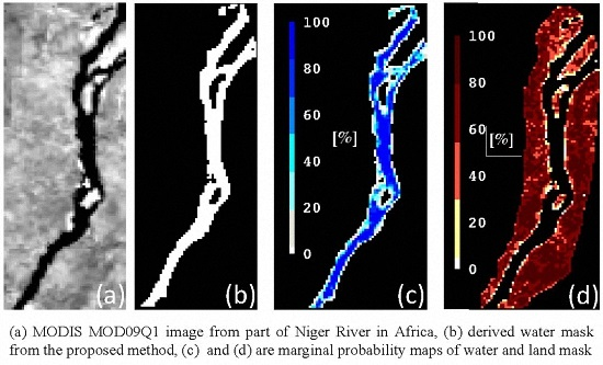
• Solve the optimization using graph cuts technique;
• Measure the uncertainty associated with the graph cuts solution;
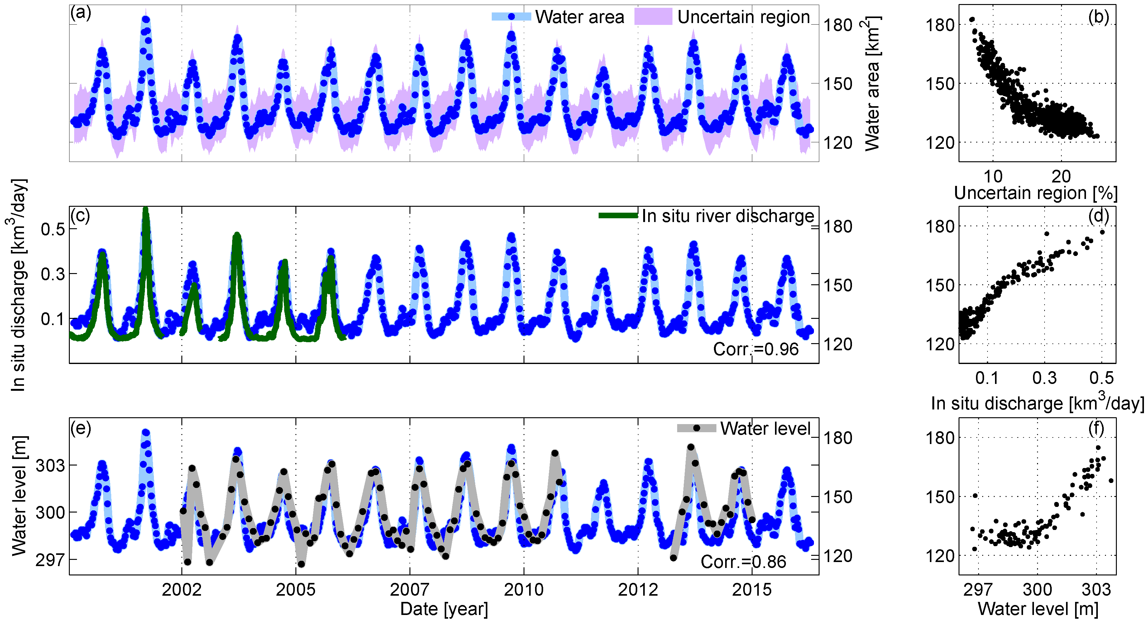
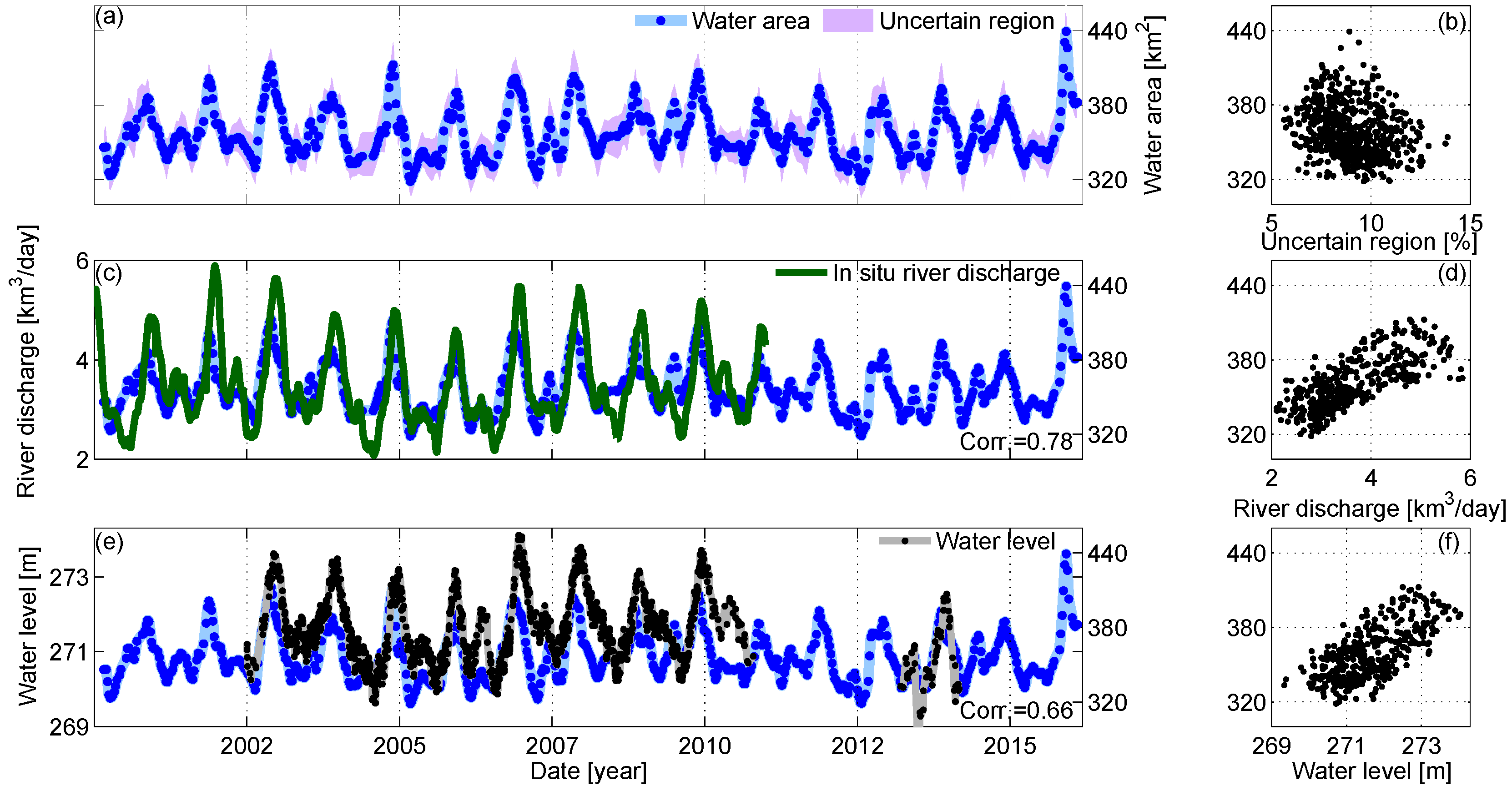
• Validate the measured water area time series indirectly through in situ river discharge and altimetric water level measurements.

2. Case Studies and Datasets

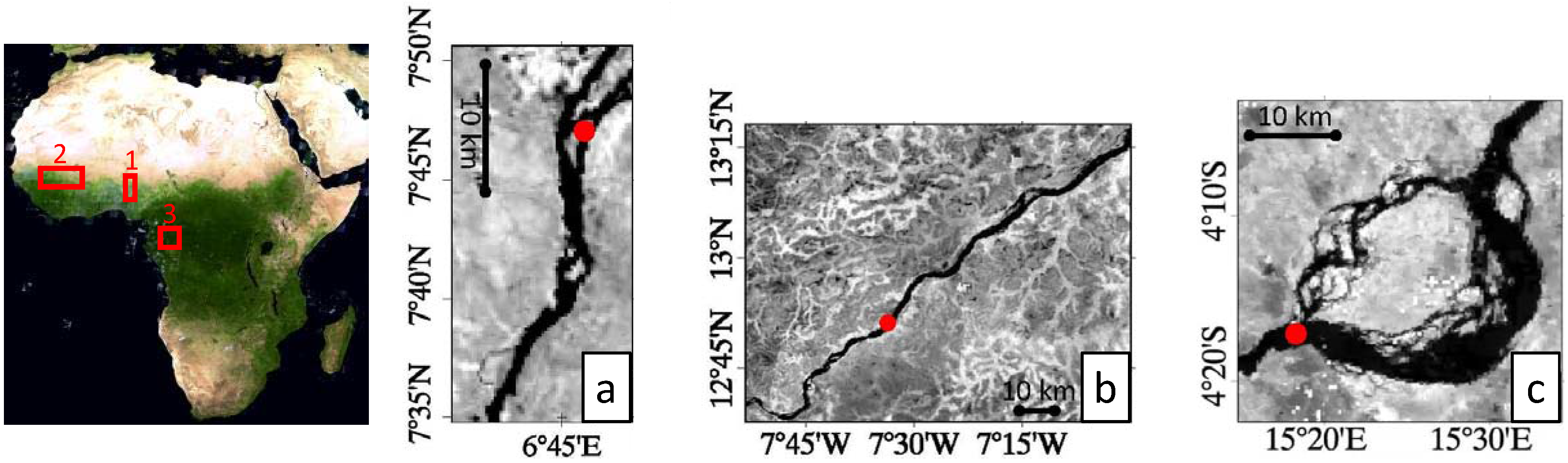
2.1. Case Study

To analyze the performance of the proposed automatic river area extraction algorithm from satellite images in different situations, we select three different river sections in Africa (Figure 2).

The first two river sections belong to the Niger River. The inland delta of the Niger River is one of the most fragile ecosystems of Sub-Saharan Africa. Patterns of land cover and land use vary extremely due to changes in the hydrological conditions of the Niger River and its tributaries. The Niger basin is comprised of very diverse ecoregions, ranging from the arid Sahel to the extremely wet coastal Niger Delta [37]. The amount of precipitation in the basin on dry and wet seasons varies significantly. Therefore, the river reach area changes with complex patterns due to the topography of the channels, the presence of vegetation, and the total amount of water filling the rivers [38].

The last case study is Malebo Pool, which is part of the Congo River located near Kinshasa. The Congo River—the second largest river in terms of catchment area in the world—has an average discharge of 41,800 m${}^3$/s [39]. The river is located in the equatorial zone, where heavy rainfall occurs throughout the year. The river area changes rapidly as a result, and monitoring the variable extent of the river and its tributaries is a challenging task.

2.2. Datasets

In this paper, in addition to satellite images, we use daily in situ river discharge and satellite altimetry water level measurements. Since there must be a one-to-one relationship between different hydrological parameters of the river, a high correlation between their times series is expected. So, we consider the correlation coefficients as a criterion for validating the water area estimations.

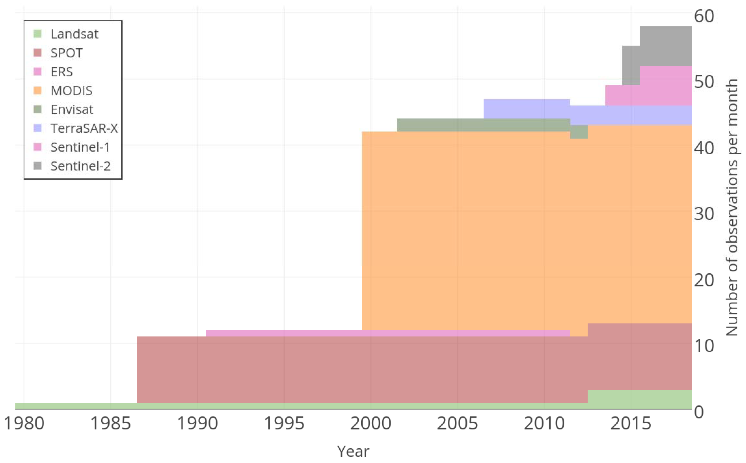
2.2.1. Imagery

MODIS images are available with daily temporal resolution globally. Most of the preprocessing has been performed by the data provider. Especially, its high-level products (levels 3 and 4) are ready to use. In this study, we use MODIS MOD09Q1, which is the surface spectral reflectance corrected for atmospheric scattering or absorption. This product is provided in two spectral bands, red and near-infrared, with $250\mathrm{m}$ spatial resolution and 8-day temporal resolution. To derive the water mask, we use the near-infrared band. In each case study, we are dealing with nearly 700 images from 2000 to 2015; in total, we processed about 2300 images for this study.

2.2.2. In Situ Data

In this study, we used available in situ river discharge measurements from the global runoff data center (GRDC) along the Niger and Congo Rivers to validate our results.

Table 2. Information about case studies and datasets.

Case	Name	Reach Length (km)	In Situ Discharge				Altimetry
			Station	Lat (${}^{\circ }$)	Lon (${}^{\circ }$)	Period	Lat (${}^{\circ }$)	Lon (${}^{\circ }$)	Period	Mission
1	Niger	20	Lokaja	${7.80}^{\circ }$N	${6.77}^{\circ }$E	2000–2006	${6.65}^{\circ }$N	${6.65}^{\circ }$$\mathrm{E}$	2003–2011	Envisat
2	Niger	115	Koulikoro	${12.87}^{\circ }$N	${7.55}^{\circ }$W	2000–2006	${12.74}^{\circ }$N	${7.73}^{\circ }$$\mathrm{W}$	2002–2015	Envisat, SARAL
3	Congo	50	Kinshasa	${4.30}^{\circ }$S	${15.30}^{\circ }$E	2000–2010	${4.28}^{\circ }$S	15.30${}^{\circ }$E	2002–2014	Envisat, SARAL

lists the location and available time period of these in situ data.

2.2.3. Satellite Altimetry

In addition to in situ data, we also validate our results against water level time series derived from satellite altimetry. Over the past two decades, satellite altimetry has been used as a monitoring tool for inland water bodies [2,20]. It has been demonstrated that altimetric water time series over rivers can sensibly be used for hydrological studies [30].

In this study, water level time series at the crossing location of altimetry groundtrack and river water body—the so-called virtual station—are achieved by employing the standard processing scheme of altimetry data for hydrological applications. There, we carefully defined the virtual stations using imagery data and relied on the measurements processed by Ice-1 algorithm [30,40,41]. Table 2 lists the location of selected virtual stations, over which the altimetric water level time series are generated. For the Congo River, we used the densified water level time series generated by Tourian et al. in [30], for which ten virtual stations of Envisat and ten of Satellite with ARgos and ALtiKa (SARAL/AltiKa) are temporally used. For the river sections along the Niger River, we used time series of a single virtual station.

3. Methodology

Markov Random Fields provide a convenient prior for modeling spatial (or temporal) interactions between pixels [42]. MRF was first introduced into image analysis by Geman and Geman in [43], and subsequently in several studies [44,45,46,47]. MRF is quite popular in remote sensing because of its ability to integrate information related to pixel intensity and spatial correlation. MRF, as an advanced technique, is applied to extract the change in satellite images [48]. Additionally, integration of temporal [49] and spatio-temporal [50] information to the Markov model are proposed. A hybrid multi-contextual MRF for flood detection SAR images is presented in [51]. Generally, the object is recognized from the background of the image using maximum a posteriori estimation on a MRF. The problem of finding the MAP estimation is usually solved by describing an energy function specified toward the problem. Then, looking for a labeling structure of the pixels, the defined energy function is minimized.

A number of search methods are commonly applied to solve energy minimization problems. Simulated annealing (SA)—an efficient global optimization technique—is widely used for this purpose [43]. However, in practice, SA is time-consuming and it does not guarantee that the final result is the global minimum [42]. Graduated nonconvexity is used as an alternative to SA. Iterated conditional modes (ICM) [52]—a local energy minimization—is also another approach to find the best labels for the segments [51]. ICM is highly sensitive to the initial estimates due to the huge number of local minima [53].

Greig et al. [54] presented for the first time how to find the global minimum of a certain energy function by applying the so-called graph cuts technique for a two-dimensional energy function. They proved that finding the minimum cost cut is equivalent to the maximum flow in a two-terminal graph. The Greig approach is the backbone of a number of efficient maximum flow algorithms recently developed, such as those presented in [47,55,56]. In the literature, graph-based minimization problems are widespread in different vision applications, such as image segmentation [44,57], stereo [46,58], shape reconstruction, and object recognition.

In this section, we start our discussion by justifying that maximizing the a posteriori estimation in an MRF and minimizing the defined energy function are equivalent. Then, to minimize the energy function, we take advantage of the graph cuts method. In the second part of this section, some basic notations and definitions of graph theory are provided. Subsequently, we describe the most common search algorithms to solve the maximum flow (minimum cut) in the graph. In the third part, we describe a method for the measurement of the uncertainty of the pixel’s label, developed by Kohli and Torr in [59]. Finally in the last section, we describe the details of our proposed setup for the river area monitoring algorithm. In this paper, we follow the definitions and notation presented in [42,60] and their followings papers.

3.1. An Overview of the Mathematical Concept

Markov Random Fields are defined in several ways in different disciplines. In the image processing community, MRF properties are usually defined as follows:

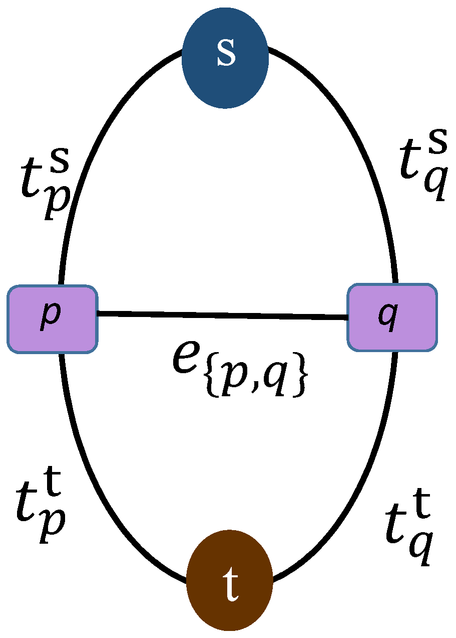
$\mathcal{P}=\{1,2,\dots ,m\}$:	a set of sites p (pixels).
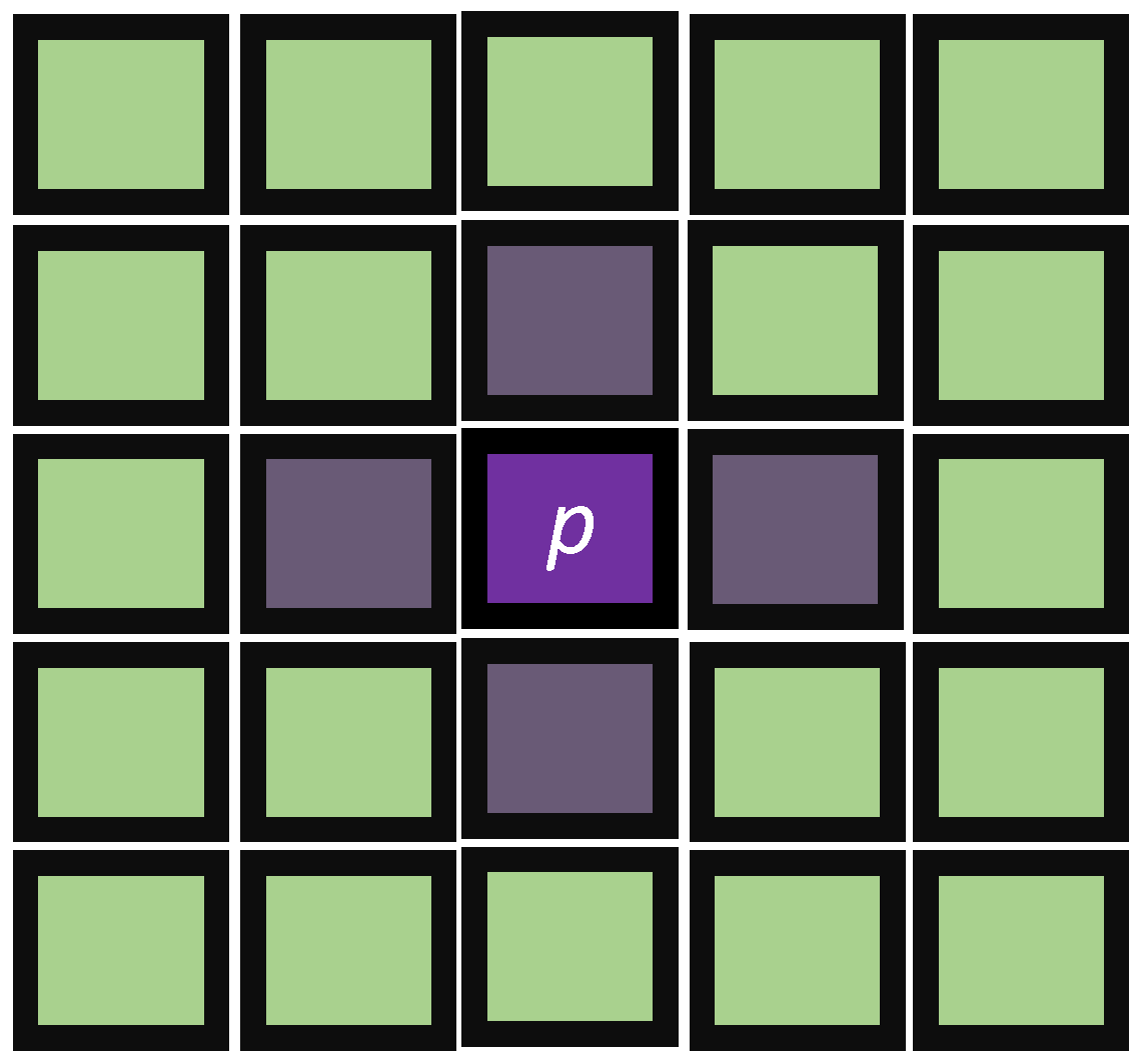
$\mathcal{N}=\left\{{\mathcal{N}}_p\right|p\in \mathcal{P}\}$:	a neighborhood system where ${\mathcal{N}}_p$ is a subset of the pixels in $\mathcal{P}$ located adjacent to the pixel p (Figure 3 is an example of a four-neighbor structure for pixel p). To provide a smoother result, one can think of a bigger neighborhood system.
$\mathcal{L}=\{l_1,l_2,\dots ,l_k\}$:	the set of possible labels that can be assigned to a pixel (water or land).
$F=\left\{F_p\right|p\in \mathcal{P}\}$:	a field of the random variables which takes a value $f_p$ regarding the possible label l.

A particular realization of the field is given by $f=\{f_p\mid p\in \mathcal{P}\}$. It is called a configuration of the field F. In order to be an MRF, all $f\in F$ must satisfy

$$\mathrm{P}\left(f\right)>0$$

(1)

$$\mathrm{P}(f_p\mid f_{\mathcal{P}-\left\{p\right\}})=\mathrm{P}(f_p\mid f_{{\mathcal{N}}_p}),$$

(2)

where $\mathcal{P}-\left\{p\right\}$ denotes the set difference, $f_{{\mathcal{N}}_p}$ denotes all labels of subset ${\mathcal{N}}_p$. This condition indicates that a pixel is only directly dependent on its neighbors. An MRF is usually specified by a joint distribution. The Hammersley–Clifford theorem provides a convenient way to define an MRF [61] by proving that MRFs and Gibbs random fields are equivalent. This theorem also states that the probability of a particular configuration is defined as:

$$\mathrm{P}\left(f\right)=Z^{-1}\exp \left(-\sum _{c\in C}{V}_c\left(f\right)\right),$$

(3)

where Z is a normalizing constant and C is the set of all cliques. A set of sites (pixels) is called a clique if every two separate pixels are adjacent. Here we just consider cliques of size two in a neighboring system. $V_c\left(f\right)$ is called the clique potential function

$$V_c\left(f\right)=V_{\{p,q\}}(f_p,f_q),$$

(4)

where $V_{\{p,q\}}(f_p,f_q)$, the neighbor interaction function, measures the similarity of two neighbor pixels p and q in terms of their labels and values. Now, we rewrite Equation (3), which is an MRF with the joint distribution

$$\mathrm{P}\left(f\right)=Z^{-1}\exp \left(-\sum _{\{p,q\}\in \mathcal{N}}{V}_{\{p,q\}}(f_p,f_q)\right).$$

(5)

The field F is not directly observable, but we can find a relationship between any realized configuration f and an observation; for example, d, via the likelihood function $\mathrm{P}(d\mid f)$. In most studies, this problem is solved using Bayes’s theorem. The posterior probability can be written as

$$\mathrm{P}(f\mid d)=\frac{\mathrm{P}(d\mid f)\mathrm{P}\left(f\right)}{\mathrm{P}\left(d\right)}.$$

(6)

The MAP estimate $f^{*}$ of f maximizes the likelihood function

$$f^{*}=arg\underset{f\in F}{max}\mathrm{P}(d\mid f)\mathrm{P}\left(f\right).$$

(7)

To find the solution, we need a model for $\mathrm{P}(d\mid f)$. If $d_p$ is the pixel value at pixel p, then we assume that

$$\mathrm{P}(d_p\mid f)=\prod _{p\in \mathcal{P}}\mathrm{P}(d_p\mid f_p).$$

(8)

When the noise is independent at each pixel, then

$$\begin{array}{c}\hfill \mathrm{P}(d_p\mid l)=C_{p}exp(-D_p\left(l\right)),l\in \mathcal{L}.\end{array}$$

(9)

In this equation, $C_p$ is a normalizing constant and $D_p\left(l\right)$ is a non-negative function which reveals how much the assigned label l agrees with the pixel value p. So, the likelihood function is equal to

$$\mathrm{P}(d\mid f)\propto exp\left(-\sum _{p\in \mathcal{P}}{D}_p\left(f_p\right)\right)$$

(10)

Now, by deriving $\mathrm{P}\left(d\right)$ and $\mathrm{P}(d\mid f)$ with the above assumption, we can rewrite Equation (7)

$$f^{*}=arg\underset{f\in F}{max}\exp \left(-\left(\sum _{p\in \mathcal{P}}{D}_p\left(f_p\right))+\sum _{\{p,q\}\in \mathcal{N}}{V}_{\{p,q\}}(f_p,f_q)\right)\right).$$

(11)

To find $f^{*}$, we must maximize Equation (11), which is equivalent to minimizing the following equation:

$$E\left(f\right)=\sum _{p\in \mathcal{P}}{D}_p\left(f_p\right)+\sum _{\{p,q\}\in \mathcal{N}}{V}_{\{p,q\}}(f_p,f_q)=E_{\mathrm{data}}\left(f\right)+E_{\mathrm{smooth}}\left(f\right).$$

(12)

This equation is the general energy function in the energy-based optimization method in image processing. The first term of the equation, $D_p\left(f_p\right)$, is a function that just deals with the pixel value and its possible label. The second term, $V_{\{p,q\}}(f_p,f_q)$, is a function that measures the agreement between two adjacent pixels in terms of their value. For convenience, we introduce a balancing term into Equation (12):

$$E\left(f\right)=(1-\lambda )E_{\mathrm{data}}\left(f\right)+\lambda E_{\mathrm{smooth}}\left(f\right)$$

(13)

where the balancing term $\lambda \in [0,1]$ allows us to control the contribution of each term to the total energy. If λ is small, the role of the neighbor interaction between pixels is not considered, so the final result only relies on the pixel intensities. On the other hand, if λ tends to 1, we ignore the contribution of pixel values in the process of segmentation and rely only on the structure of the pixels. Defining an appropriate λ is one of the most challenging parts of the problem of finding the minimum energy solution.

To minimize the energy function E, we need to find the best labeling structure for the pixels. Graph cuts have proven to be a useful multidimensional optimization tool, able to enforce piecewise smoothness while preserving relevant sharp discontinuities [62]. Here we briefly discuss the mathematical background of the problem. For complementary details, we suggest the reference book by Li [63].

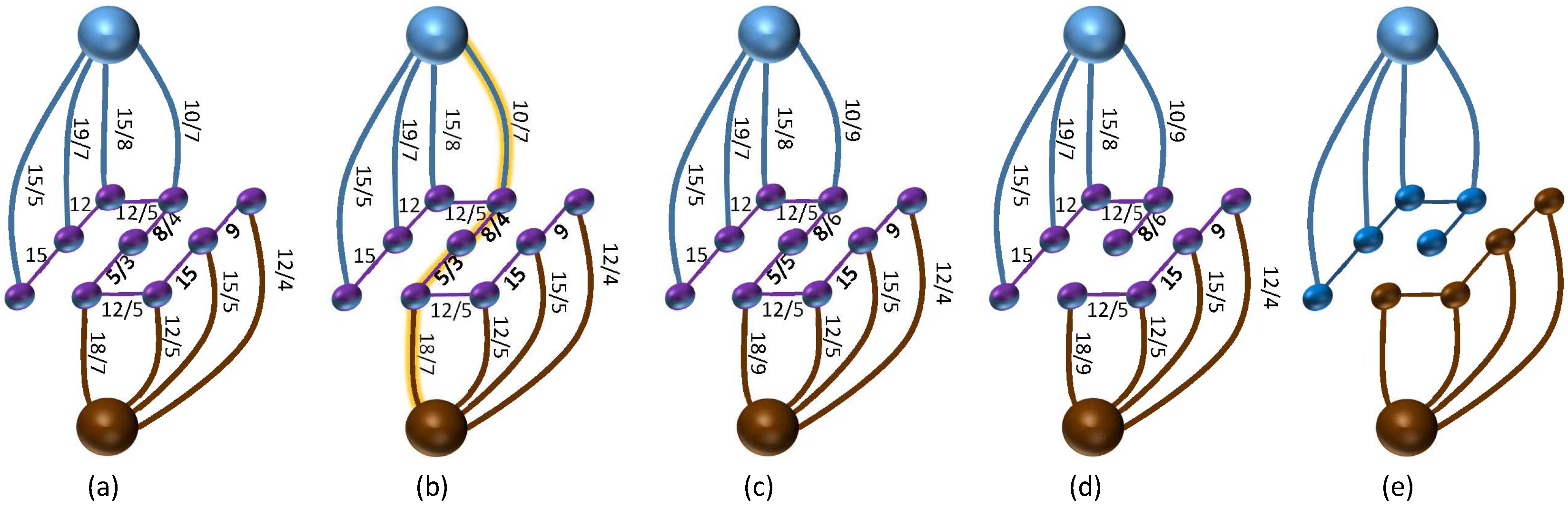
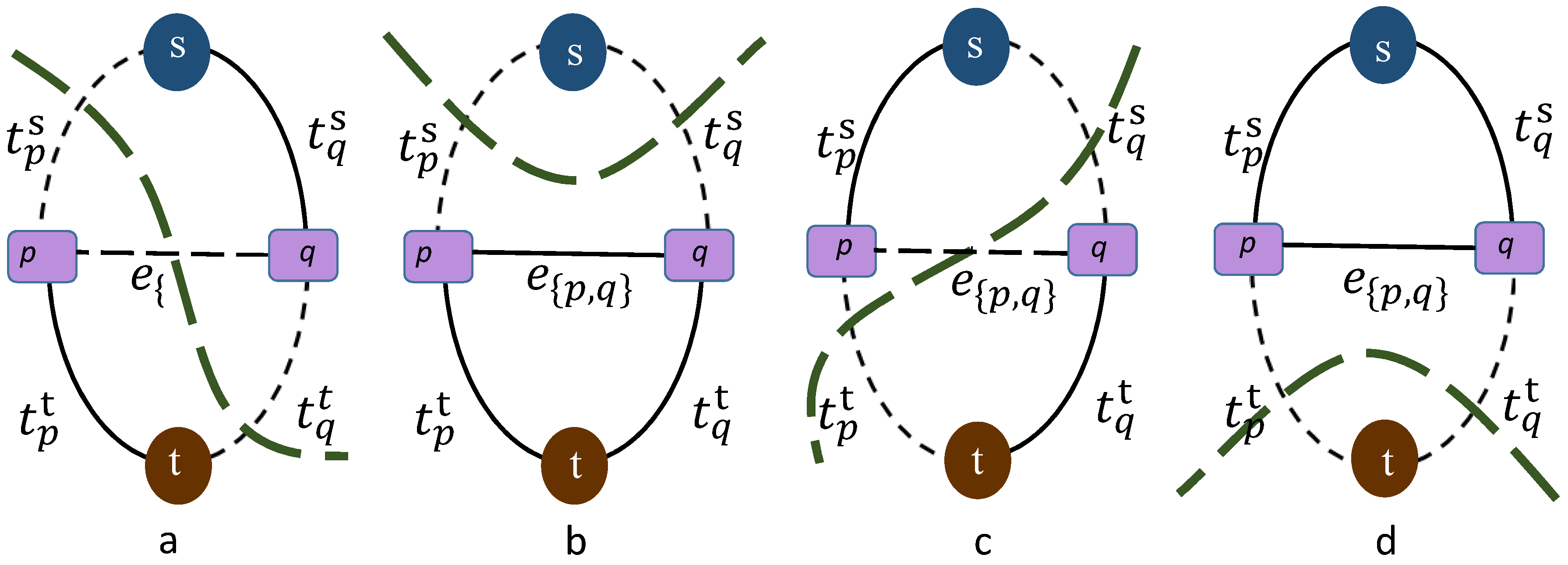
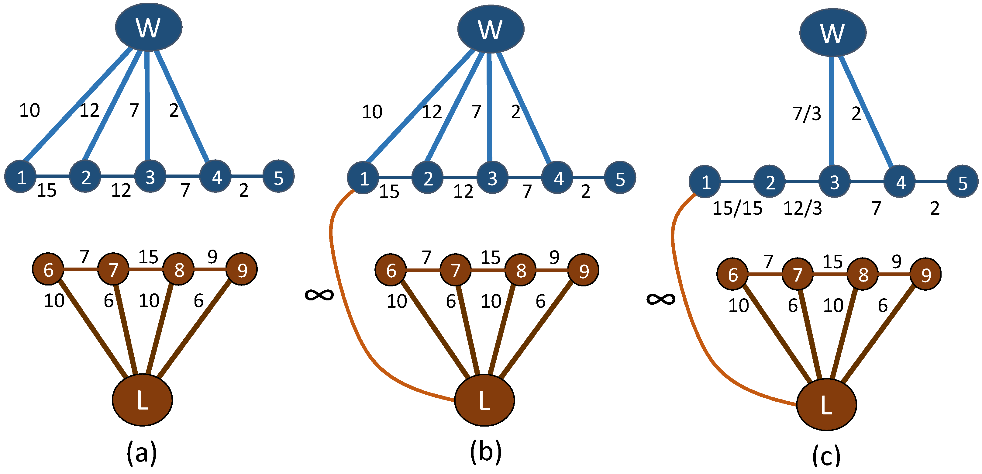
3.2. Basics of Graphs, Graph Cuts Techniques, and Max-Flow Algorithms

Here, we briefly introduce some concepts of graph, and then provide an overview of the graph cuts technique. $\mathcal{G}=〈\mathcal{V},\mathcal{E}〉$ is an undirected weighted graph, where $\mathcal{V}$ is the set of vertices. In the image application, it includes all pixels of the image, together with two additional vertices, called terminals (source and sink). The lines that connect neighboring vertices are called edges ($\mathcal{E}$). The edges that connect vertices to the terminals are called terminal links (t-links), the edge that connects two neighbor vertices is named neighbor link (n-link)—see Figure 4.

In order to assign weights to the edges, we consider the defined functions in the previous section. In each graph, t-links connect vertices to the terminal. For example, $t_p^{\mathrm{s}}$ establishes the connection between pixel p and terminal s, so its value must indicate how much the pixel value agrees with this label. The result of the function $D_p\left(\mathrm{s}\right)$ exactly measures the agreement. On the other hand, the n-link $e_{\{p,q\}}$ must describe the likeness on the values of p and q, which is the output of the function $V_{\{p,q\}}(l_p,l_q)$.

Now, to find the solution that minimizes the energy in the graph, we define a cut in the graph. The properties of a cut are discussed in [47]. A cut $\mathcal{C}$ is a set of edges in the graph which separates the graph into two discrete graphs such that every vertex connects to just one terminal via a t-link in the new configuration of the graph. The cost of each cut is equal to the sum of the weights of all edges that are available in the cut. The goal of the min-cut solution is to find the cut with the smallest cost. For example, in Figure 5, to define the label of pixels, the total cost of all possible cuts must be calculated. Then, the labels will be defined regarding the cut which has the minimum cost.

The most common techniques to find the min-cut solution take advantage of the primary fact in combinatorial optimization that the min-cut problem can be solved by finding the maximum flow from source to sink [55]. If the edges in the graph are considered as water pipes with a capacity equal to the edge weights, then we are searching for the maximum amount of water that can be sent from one terminal to the other. Maximum flow saturates a set of edges. The primary graph will be divided into two separate graphs if the saturated edges are eliminated. In fact, the maximum flow value is equal to the cost of the minimum cut [55].

Most of the algorithms used to solve the min-cut or max-flow problem with two terminals are based on two general methods: Ford–Fulkerson style augmenting paths [64] and Goldberg–Tarjan style push-relabel [65]. Augmenting paths algorithms repeat the following steps until at least one of the edges in all possible paths between source and sink is saturated. First, in the initial phase, a residual graph identical to the original graph is defined. Additionally, before starting the iteration, the flow from source to sink is equal to zero. The iteration runs as follows:

• Find a valid route between source and sink.
• Push the maximum flow equal to the capacity of the pass to the graph. This flow saturates an edge in the pass.
• Decrease the capacity of the path edges in the residual graph and increase the maximum flow regarding the previous step.

The iteration will be terminated if the algorithm can no longer find an unsaturated path from source to sink in the residual graph. At this stage, the flow is equal to the maximum capacity of the graph. Figure 6 is an example of a graph with nine vertices in the last iteration. After saturating the last s-t path, the final labels for the vertices are defined.

Push-relabel-based algorithms find the maximum flow in a completely different approach. Instead of pushing a feasible flow through the graph, the algorithm pushes the maximum possible flow from source to sink, called preflow. During its way, the preflow satisfies the capacity of passing edges and saturates them. This means that every vertex has more incoming flow than outcoming flow. At the end, the excess flow in all vertices is zero. At this point, the preflow turns to feasible flow.

To find the MAP of the MRF, we take advantage of min-cut (max-flow) solutions. The Dinic algorithm will be applied to find the maximum flow between the terminals. The Dinic algorithm is a powerful technique for computing the maximum flow in a network (graph), introduced in [66]. This algorithm belongs to the class of augmenting path techniques and increases the flow in the graph iteratively until saturation of all the s-t paths is achieved. In this algorithm, the graph is organized into different layers in a way that the first layer includes all vertices connected to one of the terminals—for example, w (water). The remaining vertices are divided into subsequent layers according to their vicinity to the vertices located in the prior layers. Then, all the paths with the shortest length are saturated by applying breadth-first search (BFS). Given the vertex p in the graph $\mathcal{G}$, the BFS lists all the vertices located at distance k from p, and then in the next layer, it finds every vertex at distance $k+1$. The Dinic algorithm repeats the following steps until saturating the last s-t path.

• Find all paths from source to sink with length k in the residual graph applying BFS
• Augment the detected paths, update the residual graph, increasing the total flow
• Replace k with k+1

At the first step, the total flow is equal to zero, and the assumed length of the s-t shortest path (k) is also zero. Every iteration starts with a new BFS with the increased length regarding the previous step. After augmenting all the possible paths between terminals, we define the label for each pixel by applying a depth-first search (DFS) in the final residual graph. Finally, based on the assigned labeling structure for the pixels, the modified water masks will be defined.

For the generation of a reliable water mask time series, apart from finding the most possible configuration of labels for the pixels, providing additional information (such as marginal probability) for each pixel assigning a certain label is essential. Measuring the uncertainty of the assigned labels plays a critical role in generating an accurate water mask, since the exact river area is not available in our study.

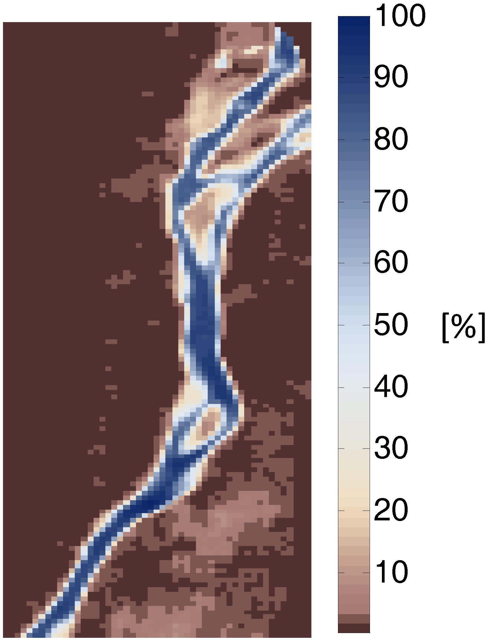
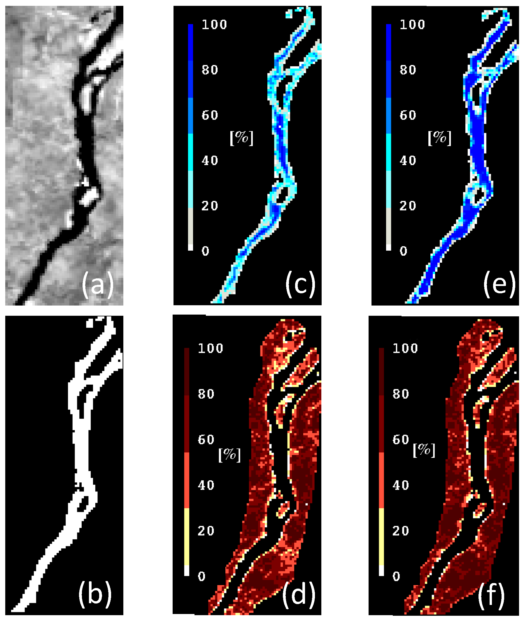
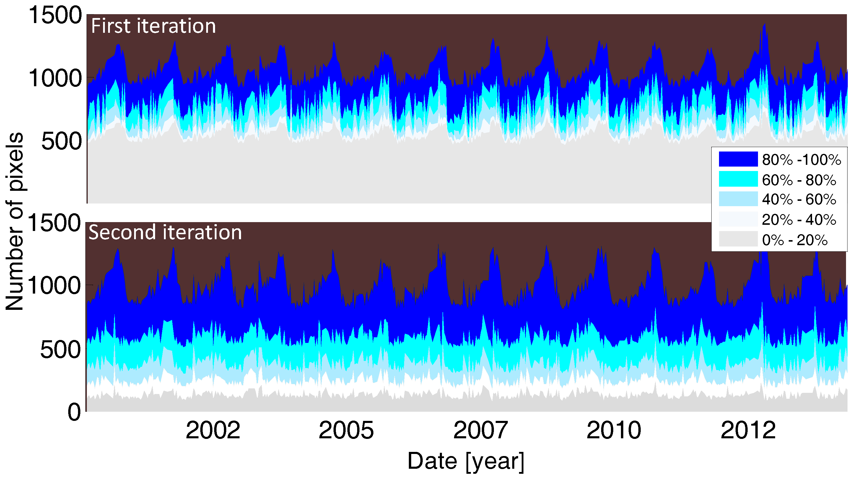
3.3. Measuring Uncertainty in the Graph Cuts Solution

Unlike other inference algorithms, such as Loopy Belief Propagation, Generalized Belief Propagation, and Tree-ReWeighted Message Passing, graph cuts suffer from a disadvantage. They do not provide any uncertainty measure associated with the determined labeling structure for the pixels [67]. However, graph cuts are preferred over other algorithms, and they have been extensively used for various computer vision problems that deal with computing the MAP solution [59]. The main reason is their ability to find a globally optimal solution in polynomial time. Even in problems where the availability of a global optimum solution is not guaranteed, graph cuts can find the most appropriate local minimum in the graph [46,59].

To overcome this deficiency, Kohli and Torr in [67] introduced a method to measure uncertainty in graph cuts solutions. Here we provide only a brief review of their method, and do not mention details. Details and mathematical concepts are described in [67,68].

Kohli and Torr (KT) presented minimum marginal energy associated with the label assignments of any latent variable in a MRF. A min-marginal energy is a function that provides information about the minimum values of the energy function E under different constraints. So, the function min-marginal energy ${\psi }_{p;l}\left(\theta \right)$ is defined as

$${\psi }_{p;l}\left(\theta \right)=\underset{f\in \mathcal{F},l_p=l}{min}E(f\mid \theta ).$$

(14)

In this function, θ is the energy parameter related to the fields. For example, we know that the value of the energy function E depends on the selected realization of the fields ($f\in \mathcal{F}$). To measure the min-marginal energy for a certain pixel (e.g., p), we can assume that its label ($l_p$) is fixed, and then try to minimize the function E over the rest of the pixels. The minimum value obtained for the function in this case is the min-marginal energy for the pixel p, which leads to the label $l_p$.

To find a relationship between min-marginal energy and confidence measurement for the assigned label, a function $\mathrm{p}(f\mid \mathbf{D})$ is defined. This function specifies the probability of a realization of the MRF. The max-marginal, ${\mu }_{p;l_p}$, gives us the value of the maximum probability over all possible configurations of the MRF in which $p=l_p$. Formally, it is defined as

$${\mu }_{p;l}=\underset{f\in \mathcal{F};l_p=l}{max}\mathrm{P}(f\mid \mathbf{D})$$

(15)

Now, max-marginal measurement can be normalized to obtain a confidence measure σ for any pixel-assigned label regarding the labeling configuration [67].

$${\sigma }_{p;l}=\frac{{max}_{f\in \mathcal{F};f_p=l}\mathrm{P}(f\mid \mathbf{D})}{{\sum }_{k\in \mathcal{L}}{max}_{f\in \mathcal{F},f_p=k}\mathrm{P}(f\mid \mathbf{D})}=\frac{{\mu }_{p;l}}{{\sum }_{k\in \mathcal{L}}{\mu }_{p;k}}$$

(16)

So, if the pixel p takes the label l, then ${\sigma }_{p;l}$ indicates the uncertainty of the labeling assignment for this pixel. Since in this study we deal with a binary image segmentation problem with two labels ($\mathcal{L}=\{\mathrm{l},\mathrm{w}\}$), Equation (16) is reshaped into

$${\sigma }_{p;\mathrm{w}}=\frac{{\mu }_{p;\mathrm{w}}}{{\mu }_{p;\mathrm{w}}+{\mu }_{p;\mathrm{l}}},{\sigma }_{p;\mathrm{l}}=\frac{{\mu }_{p;\mathrm{l}}}{{\mu }_{p;\mathrm{w}}+{\mu }_{p;\mathrm{l}}}.$$

(17)

The relationship between max-marginal probability and min-marginal energy for any pixel (like p) given a label (l) is

$${\mu }_{p;l}=\frac{1}{Z}\exp (-{\psi }_{p;l}\left(\theta \right)),$$

(18)

in which Z is the partition function. Thus, we are able to reshape Equation (17) using min-marginal energies

$$\begin{array}{c}\hfill {\sigma }_{p;\mathrm{w}}=\frac{\exp (-{\psi }_{p;\mathrm{w}}\left(\theta \right))}{\exp (-{\psi }_{p;\mathrm{w}}\left(\theta \right))+\exp (-{\psi }_{p;\mathrm{l}}\left(\theta \right))},\end{array}$$

(19)

which shows that, to measure the uncertainty of a label assigned to a pixel, we need only measure the pixel min-marginal energy in the graph. In the max-flow problem, min-marginal energy for any pixel is equal to the sum of the maximum flow and pixel flow potential in the final residual graph ($\mathcal{G}\left(f^{*}\right)$) [67].

Maximum flow is the sum of the flow passed from source to sink, leading to saturate some edges and disconnect all the available paths between two terminals. Flow potential defines separately for each node in the final residual graph. Let us assume that label w (water) is assigned to the pixel p by the graph cuts solution. This means that in the residual graph, p connects to the terminal water directly with a t-link or via its neighboring pixels. On the other hand, there is no connection between p and the terminal land. Since $f^{*}$ represents the MAP solution, the flow potential of pixel p related to the land label is zero ($C_p^{\mathrm{l}}=0$). Now, to define the flow potential for p related to its label, we add a t-link between p and terminal land with infinite weight ($t_p^{\mathrm{l}}=\infty$). By adding this imaginary edge, the connection between source and sink is established again. After augmenting all the possible s-t paths considering the new t-link, the flow-potential for p is equal to the sum of the flow capacity of all new paths. Figure 7 is an example of described procedure.

By measuring the min-marginal energy and max-marginal probability for all the water mask pixels—apart from a binary water-land mask—a probabilistic water mask can be generated as a grayscale image to illustrate the probability for each pixel assigned as water. In our cases, we expect low probability for the pixel located around shorelines, and high probability for the pixel located in the middle of the river.

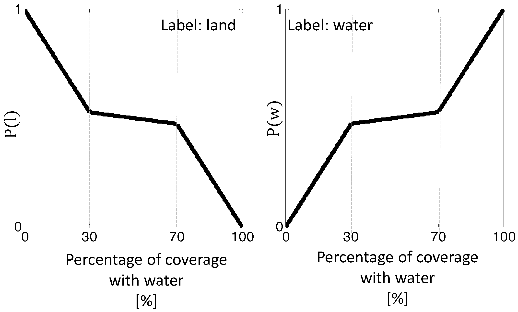
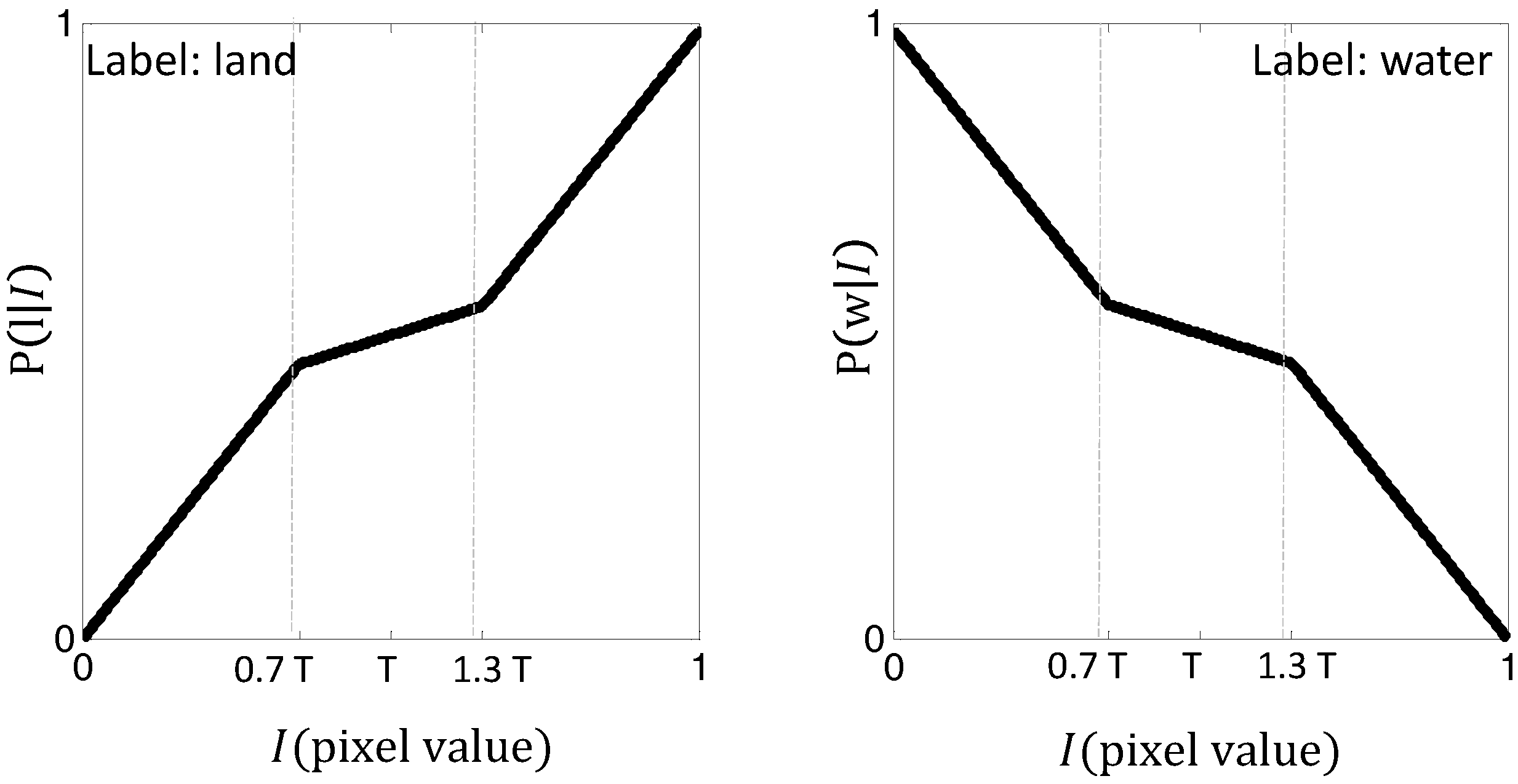
3.4. Implementation of Energy Functions

In addition to selecting the max-flow algorithm, the careful definition of the energy function components (13) is also critical. This equation includes two weight functions (pixel value weight function, neighboring interaction weight function) and one constant value. If the weight functions are defined properly, all the s-t paths will be found and saturated in a few iterations of the procedure, because only a small fraction of vertices located around shorelines are involved in the process. In other words, while a simple threshold on the image histogram is able to assign a reliable label to the majority of pixels, the algorithm will focus on the critical areas (shallow water and shorelines) to detect the correct labels. The target area is relatively small, so it is possible to block all possible s-t paths in a limited number of iterations.

In general, there is no restriction for defining the $D_p$ function [42]. Kolmogorov et al. [58] state that in a binary labeling structure ($\mathcal{L}=\{0,1\}$), satisfying the condition

$$V_{\{p,q\}}(0,0)+V_{\{p,q\}}(1,1)\le V_{\{p,q\}}(1,0)+V_{\{p,q\}}(0,1)$$

(20)

for the function $V_{\{p,q\}}(f_p,f_q)$ is necessary and sufficient. This property is called regularity, and plays an important role in defining the energy functions. In the max-flow problem, we consider edges as a network of pipes. So, the assigned weight for an edge is equivalent to the capacity of the pipe. We also define the weight functions for the normalized images, so the range of pixel values varies between zero and one.

As described before, $D_p\left(f_p\right)$ measures the agreement between the value of the pixel p and the label f. The function D(.) must assign a large weight to the connecting edge between the pixel and the label if the pixel value indicates the characteristic of the label. For example, if a pixel (like a) has a near-zero value in the infrared band of an optical image, then the weight of $t_a^{\mathrm{w}}$ (the t-link that connects a to the label water (w)) is larger than $t_a^{\mathrm{l}}$ (t-link connects a to the label land (l)). Since we deal with a long time series of images from the water bodies in our study, every pixel has a long-term behavior with respect to water coverage. Generating a map of frequency of water coverage after initial classification reveals the temporal statistics of each pixel. So, for a pixel p in a standard binary labeling problem, two labels are available—here water (w) and land (l). We define the $D_p\left(f_p\right)$ now as

$$D_p\left(f_p\right)=\left\{\begin{array}{c}{D}_p\left(\mathrm{l}\right)\propto \mathrm{P}\left(\mathrm{l}|I_p\right)\times \mathrm{P}\left(\mathrm{l}\right)\hfill \\ D_p\left(\mathrm{w}\right)\propto \mathrm{P}\left(\mathrm{w}|I_p\right)\times \mathrm{P}\left(\mathrm{w}\right)\hfill \end{array}\right.$$

(21)

which shows that t-links are calculated by multiplying the probability of assigning a label within the pixel value ($I_p$) with the probability of assigning the label regarding to the long-term behavior of the pixel. To calculate these probabilities, we need to determine the probability of assigning water or land to pixel ($\mathrm{P}\left(\mathrm{l}\right)$, $\mathrm{P}\left(\mathrm{w}\right)$). Thus, for each label, a separate model is developed using the water coverage map in the monitoring period (see Figure 8).

Models in Figure 8 indicate the possibility of a pixel being land or water, regarding its long-term behavior. For example, if a pixel is covered by water in more than 70% of the images, then the possibility of being water is much higher than being land for that pixel. After that, the conditional probability of the given label and pixel value ($I_p$) must be measured. To do this, we define two other models (see Figure 9); using the models, we measure the possibility of assigning a label to a pixel regarding its pixel value. For example, if a pixel has a very small value ($I_p\approx 0$), then the conditional probability of $I_p$ within the label water ($\mathrm{P}\left(\mathrm{w}|I_p\right)$) is near one, and on the other hand $\mathrm{P}\left(\mathrm{l}|I_p\right)$ is near zero.

The second part of Equation (13) measures the interaction between neighboring pixels. Here we introduce $V_{\{p,q\}}(f_p,f_q)$, which measures the cost of assigning the same label to two adjacent pixels. In general, $V_{\{p,q\}}(f_p,f_q)$ devotes a small weight to the edge between connected pixels with a big difference in their pixel value. On the other hand, the weight assigned to the connecting edge between two pixels with similar value is large. Based on the long-term behavior of pixels, we can also measure the possibility of assigning the same label for a pair of pixels connected with an n-link. First, to define $V_{\{p,q\}}(f_p,f_q)$, we introduce an event the Q, in which two pixels have the same label. To measure the probability of this event (P(Q)), we can take advantage of the models introduced in Figure 8.

Since our problem is categorized as a piecewise smooth prior (Figure 10b), n-links must be defined in a way that handles the discontinuities in the image by setting appropriate weights for the boundaries. To this end, we first introduce $w_{pq}$ as a function of pixel values connecting via the n-link

$$w_{pq}=\frac{{(I_p-I_q)}^2}{2{\sigma }^2},$$

(22)

in which $I_p$ and $I_q$ are the pixel values, and ${\sigma }^2$ is the variance of pixel values over the whole image. Next, we define the cost of the neighboring interaction between two adjacent pixels.

$$V_{\{p,q\}}(f_p,f_q)\propto \exp (-w_{pq})\times \mathrm{P}\left(\mathrm{Q}\right)$$

(23)

This function assigns a large weight for an n-link connected two pixels with almost the same pixel value and temporal behavior. It assigns a small weight to adjacent pixels with a significant difference in their pixel intensities.

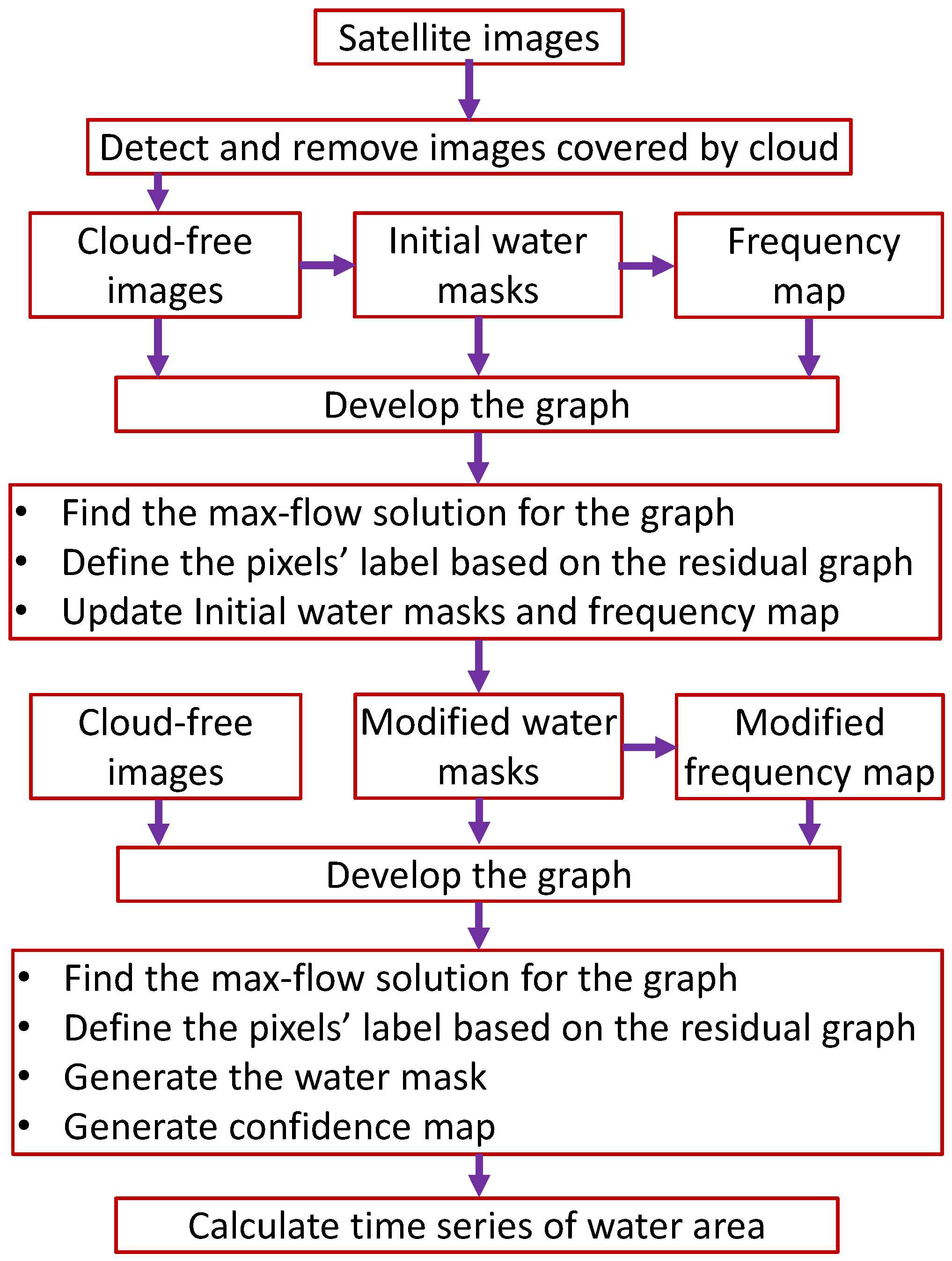
3.5. Review of the Proposed Method

The procedure of generating water area time series is presented in the flowchart in Figure 11.

The algorithm starts by expelling the images covered with clouds. They not only impose a wrong water area estimation, but also spoil the area estimation in other epochs, since the temporal behavior contributes to the weight functions. Apart from visual interpretation, an automatic algorithm to precisely detect clouds in the optical images—especially in a single spectral band—is difficult to achieve. We apply two filters to detect cloud-free images. First, we assume that consecutive images nearly look alike because the time interval between them is relatively short (8 days). So, cloud cover is the likeliest reason for significantly reduced correlation between two consecutive images. For the second filter, we take advantage of the fact that the value observed for clouds in the near-infrared band is almost constant. So, the variance of the pixel values of all pixels in an image would be small if clouds cover the majority of the image. The sensitivity of these two filters is adjustable based on the situation. For example, by reducing the sensitivity, images with partial cloud cover could be accepted.

To construct the graph, we must assign weights to its edges using the weight functions introduced in this section. The primary input for calculating the n-links is pixel values of the cloud-free images, but to calculate t-links, we also need initial water masks. The third requirement for developing the graph edges is the initial frequency map developed using initial water masks.

After calculating all the edges in the graph, we now search for the optimal pixel label structure by finding the max-flow solution in the graph. To generate more accurate water masks, we repeat the river area extraction process . In the update round, however, results of the first iteration are replaced with the water masks generated in the first iteration. The frequency map is also updated with modified water masks.

The final product is a binary water–land map, so any further information about the uncertainty in assigned labels is not provided. In this way, apart from visual comparison with the original images, an evaluation of the water mask quality is not possible. For further assessment of the water masks, we measure the marginal probability for each water mask pixel applying the KT method on the residual graphs. To do this, the maximum flow for each graph is measured during the max-flow procedure. Then, min-marginal energy is calculated for each pixel based on the final residual graph. By knowing these two variables, we are now able to measure the labels’ uncertainty. The final products of the proposed method include binary and probabilistic water masks and river area time series.

4. Results and Validation

In this section, we assess the performance of the proposed method. We describe the procedure for the first case study in detail (Niger River, Lokaja station) in order to provide insight into the method.

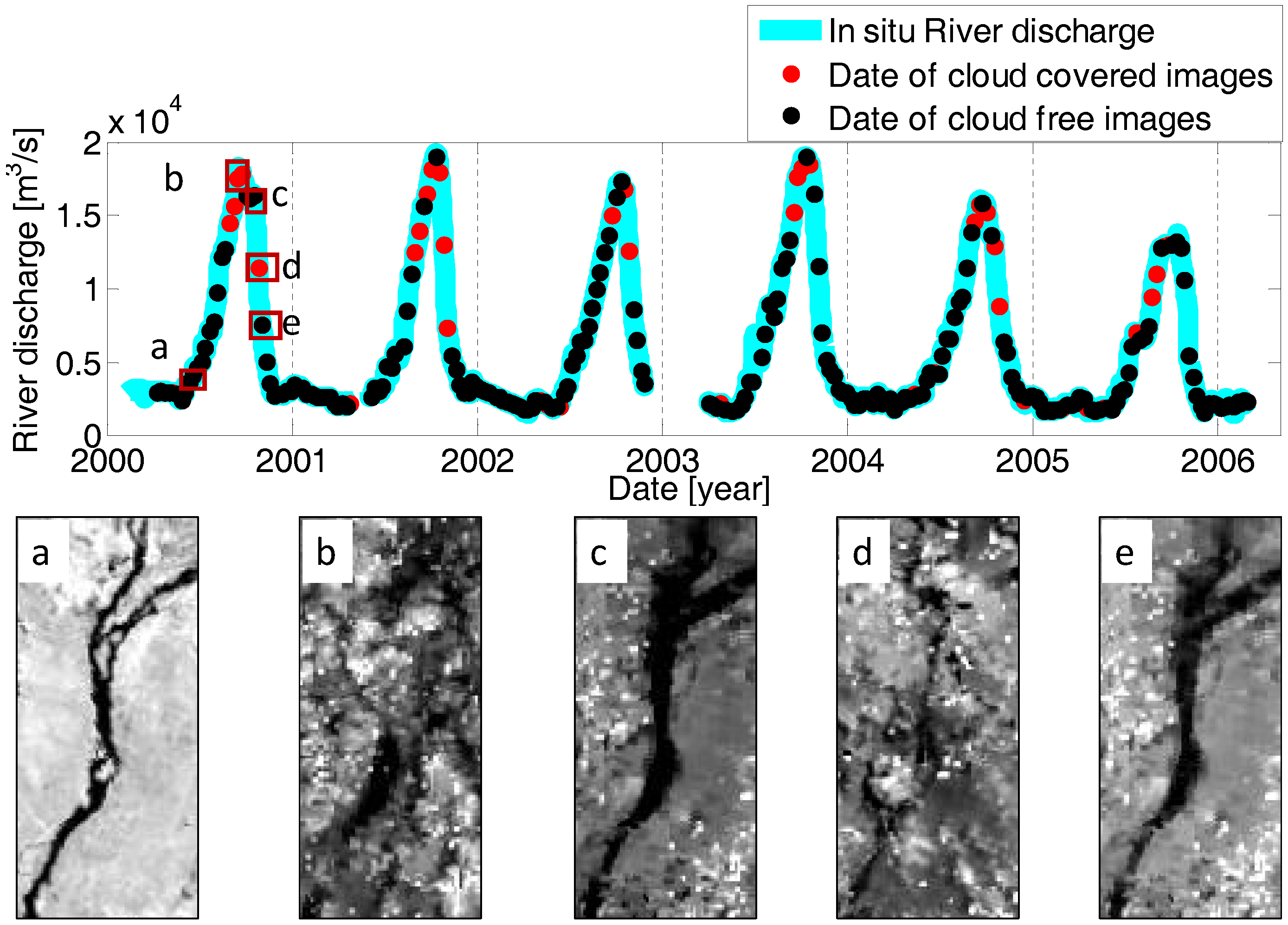
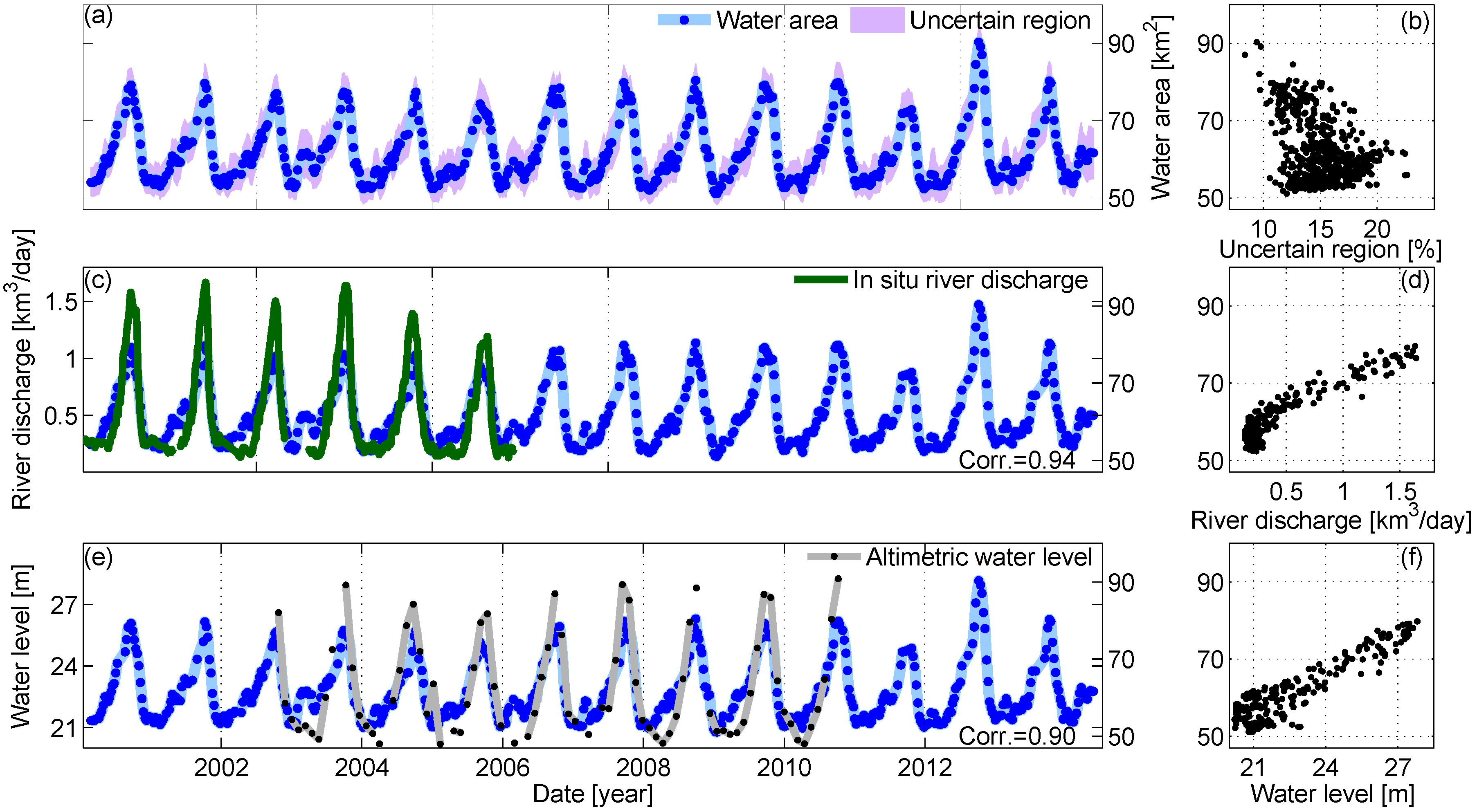
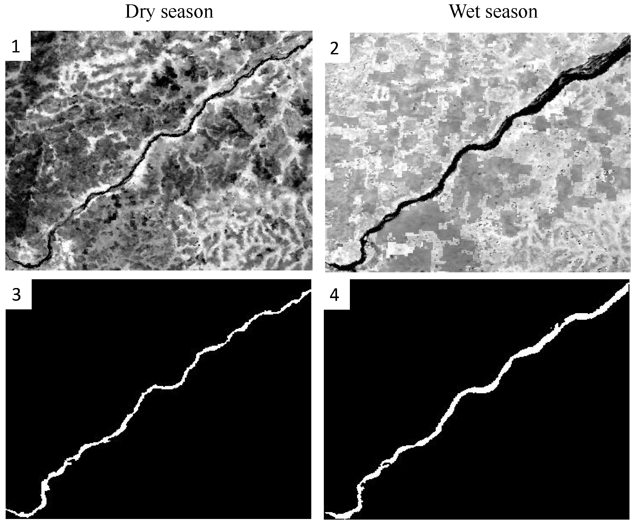
4.1. Niger River, Lokaja Station

Figure 12 shows five images of the Niger River at different months in the year 2000. The epochs are indicated on the time series of in situ river discharge (Figure 12 top).

This figure shows that cloud cover occurs more often in the wet season. Hence, eliminating cloud-covered images may lead to undersampling of the wet seasons.

Graph edges are defined with the weight functions defined in Section 3.4, for which we need an initial water mask. In order to derive the initial water mask, we apply k-means clustering. We consider the long-term behavior of the water bodies in weight functions by defining two probabilities ($\mathrm{P}\left(\mathrm{w}\right)$, $\mathrm{P}\left(\mathrm{l}\right)$) regarding the frequency coverage map. An estimation of temporal behavior for each pixel is estimated by dividing the sum of all binary water masks by the total number.

In Figure 13, dark brown pixels represent the area which is always dry, and blue ones indicate water. The critical region can be defined where the percentage varies between 30% and 70%, which are predominantly located along the river shorelines. By looking at the time series of pixel labels over these regions, we recognize an annual behavior switching between the water and land label. This means that the k-means clustering classifies them as part of the river during the wet season, and as land for the dry season.

After assigning weights to the graph edges, the max-flow solution in the graph can be sought. This step starts with repeatedly augmenting the shortest s-t paths until two terminals become completely disconnected from each other. Then, regarding the residual graph of the max-flow solution, the water mask is defined. To discuss the performance of the method, we compare four final water masks with the initial ones over the Niger River, Lokoja station (Figure 14).

Figure 14(a1) relates to the dry season, in which no cloud appears in the image, and the surrounding area is dry. As a result, the river borders are clearly distinctive. By comparing the graph cuts solution (Figure 14(c1)) with the initial water mask (Figure 14(b1)) and the original image, we find that our proposed method can accurately determine the water extent, although the improvement is small. In Figure 14(a2), the river area increases due to the increment of the water stream, and we see that the adjacent areas are also wet. As a consequence, the initial water mask (Figure 14(b2)) is not accurate, as some land pixels are labeled as water. However, the graph cuts method is able to overcome this situation to a large extent and improve the final water mask (Figure 14(c2)). Our algorithm is even able to remove most of the isolated pixels which are wrongly labeled as water in the initial water mask.

In Figure 14(a3), the land around the river border in the bottom of the river is wet, and the upper part of the river is also covered by cloud. The graph cuts method extracts the river from the surrounding wet area, and it can recover the cloudy part of the river (Figure 14(c3)). The last example reveals the ability of the method to ignore clouds and determine the water mask as accurately as possible (Figure 14(c4)). Such results indicate that the weight functions for defining graph edges are properly defined.

Next, we measure the marginal probability for each pixel in the water mask applying the KT method on the residual graph. To do this, after measuring the maximum flow passed through the graph, min-marginal energy is calculated for each pixel. By knowing these two variables, we are now able to measure the labels’ uncertainty.

Figure 15 presents an example of probabilistic water masks, in which marginal probabilities of land and water are provided. In the probabilistic water masks (Figure 15c,e), the labels of the middle part of the river section are considered accurate when their marginal probabilities are higher than 80%. Closer to the river shorelines, the level of confidence decreases. For example, in the larger part around shorelines, the marginal probability is less than 20%. The probabilistic land masks (Figure 15d,f) show the same pattern. It can be seen that pixels located far from the river have land labels with high marginal probabilities. However, closer to shorelines, the land marginal probabilities decrease. After comparing the probabilistic water and land masks of the first and second iterations, we observe that the number of pixels with high marginal probability value has improved.

Figure 16 shows the time series of marginal probabilities for the water masks of both iterations, in which the improvement after the second iteration is clearly visible. In fact, by replacing the initial water masks with the modified ones in the second iteration, just a small number of pixels have low marginal probability in the final product.

In order to generate a reliable water area time series, we estimate river area together with its uncertainty. We accept the assigned labels for pixels with marginal probabilities higher than 10% in both water and land masks. This leaves a third region which contains pixels with marginal probabilities less than 10% in both masks. This is the uncertain region, for which we cannot define a proper label based on the available information. It is clear that the area of this region correlates with the pixel size of the image. In other words, if we were to use Landsat, with a pixel size of 30 m × 30 m, the area of this region would be much smaller than in the case of using MODIS, with a coarse pixel size of 250 m × 250 m. Figure 17 represents the time series of the three different regions.

We calculate the area of a river reach by multiplying the number of pixels in the water mask by the area of a pixel. We consider the area of the uncertain region as the uncertainty of the water area measurement. Figure 18a shows the result of our method for Niger River, Lokoja station. The river section has an obvious seasonal behavior, associated with seasonal variability of precipitation. The blue dots in the time series represent the satellite observations. During the wet season, a number of images were removed due to cloud contamination. As a result, the sampling is denser during the dry season.

We analyze the uncertainty of river area estimation to understand the behavior error. Figure 18b is a scatter plot of water area vs. uncertainty. It shows that the uncertainty varies between 9% and 22%, with average uncertainty being around 15% of the area. Figure 18b shows that our algorithm estimates the water area more accurately during the wet season (when the water area is larger) than during the dry season. In the dry season, when the river becomes narrow, the middle part of the river only includes a few pixels. So, the remaining pixels in the water mask are adjacent to the dry area and have a small marginal probability. However, sometimes even during the dry season, we obtain relatively low uncertainty due to the shape of the river section.

The marginal probability for the labels is only an internal criterion for validation of the labeling. In order to assess the correctness of our river area estimation, we compare with in situ river discharge and with altimetric water level measurements. In a natural river channel, the relation between different hydraulic parameters of the river can be described by

$$\begin{array}{c}\hfill w=a{Q}^b,d=c{Q}^f,v=k{Q}^m,\end{array}$$

(24)

where Q is river discharge, d is the mean depth, w is the river width, v is the mean velocity, and the other parameters are constant values [69].

Equations (24) imply a monotonic relationship of river width with river discharge and water level. Therefore, the corresponding time series should show a significant correlation. This fact provides the opportunity to validate our water area estimations indirectly against river discharge and water level time series.

The high correlation between the two time series (0.94) in Figure 18c indicates a high consistence between the behavior of water area and river discharge. The discharge–area scatter plot (Figure 18d) shows a non-linear relationship. As expected, the area estimations during the wet season are more accurate than the dry season. In the bottom-left side of the plot, we see an irregular behavior, due to the lower performance of the algorithm or poor discharge measurements during the dry season.

Further, we compare water level with water area. To this end, we use water level from satellite altimetry, which overlaps with our water area estimation for the time period of 2002–2011 (Figure 18e). Similar to validation against discharge, the water level and water area are highly correlated (0.90). The scatter plot represents such high correlation between water area and height (Figure 18f). Like previous plots, in the wet season, the scatter of points are narrow, which indicates that both water level and area are measured accurately.

4.2. Niger River, Koulikoro Station

We have employed our algorithm over another part of the Niger River with different morphological character near the Koulikoro station. In this case, we select a long river reach of about 115 km, which has a calmer streamflow than the first case study. Figure 19 shows two examples of river water mask. In the dry season (Figure 19(1)), the average river width is less than 0.5 km, which is a challenge for our method because of the 250 m MODIS pixel size. Despite this limitation, our algorithm successfully retrieves the river extent, as it takes advantage of all possible sources of information. Additionally, in this example, since the river reach length is long, the percentage of uncertain region area with respect to the river area is decreased. Figure 19(2) is taken during the wet season, when the river area is wide enough to be precisely determined by the algorithm. Here, also due to the clear distinction between river borders and the surrounding area, the river area is measured more accurately.

In the time series of water area, we see that the river section has a clear seasonal behavior during the monitoring period (Figure 20a). The magnitude of the uncertain region in the dry season is much larger than in the wet season. By looking at the scatter plot of water area and percentage of uncertainty (Figure 20b), the clear non-linear relation between them is obvious. In the wet season, the relative uncertainty is less than 10%. By decreasing the water area, the number of pixels with high marginal probability also decreased. As a result, the uncertainty ratio percentage increases up to 25% in the dry season.

As in the previous example, we compare the in situ daily discharge with the water area of 2000–2006, which are correlated with a correlation coefficient of 0.95 (Figure 20c). As we expect, in the dry season, water area estimation is less accurate, when the water area shows a variation in spite of constant discharge. On the other hand, in the wet season, the algorithm can extract the river extent more accurately by increasing the water area. Figure 20d shows the scatter plot of simultaneous discharge and river area. The non-linear relationship between water area and discharge is evident in this plot. The wide scatter where the river discharge is less than 0.1 km${}^3$/day indicates the limitation of the method to estimate the correct water area in the dry season. The course pixel size of the MODIS images is the main reason for this problem. Finally, we compare the water area with the altimetric water level time series (Figure 20e).

In the end, a scatter plot of simultaneous altimetric water level and area measurements is presented in Figure 20e. The correlation of 0.86 is not as high as the previous case, because satellite altimetry fails to properly estimate the water level during the dry season. The vast cloud of points in the water area–level scatter plot justifies the fact that both time series do not represent water level and area of the river when river flows in a narrow channel (Figure 20f).

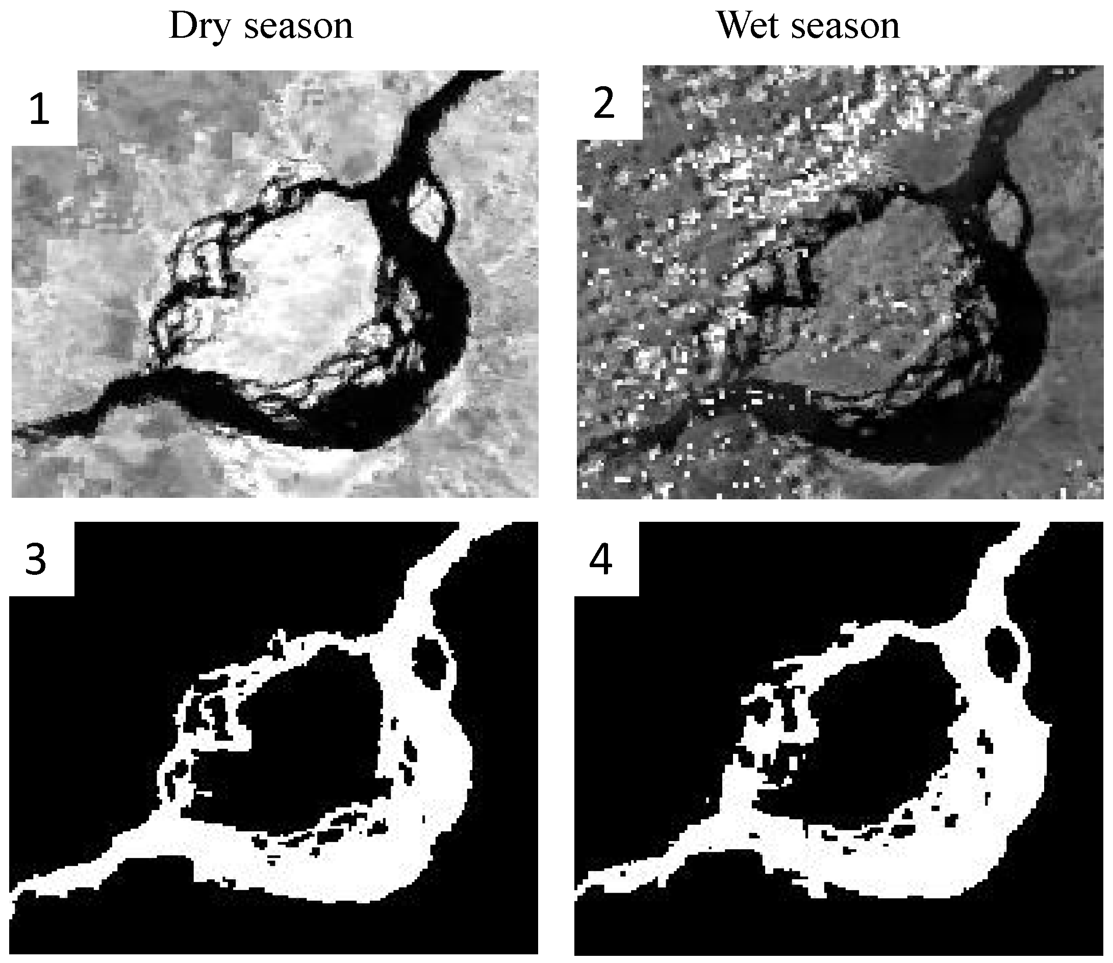
4.3. Congo River, Malebo Pool

As a last case study, we have selected a part of the Congo River near Kinshasa which has an entirely different hydrologic character and morphology from the other two cases (Figure 2). Upon leaving the Maloukou, the Congo River divides into two branches that forms a vast lacustrine area about 24 by 27 km, geographically known as Malebo Pool (Figure 2c). After flowing about 24 km, they join and pass through Brazzaville city. The amount of water flowing in this river reach is several times higher than in the previous examples. The middle part of the river contains a complex braided system, including a number of islands and narrow branches around. Due to the complexity of the river system, the area monitoring is a challenging task. Figure 21 shows two examples from wet and dry seasons.

The river section is clearly visible in most of the images in the dry season (Figure 21(1)). However, in the wet season, the majority of images are partially covered by clouds (e.g., Figure 21(2)). However, our algorithm overcomes this obstacle to a large extent by considering the temporal behavior of pixels. The extracted river mask over which the cloudy pixels are found well (Figure 21(4)). Figure 21(3) is the water mask generated out of the image in Figure 21(1). The middle part of the Malebo Pool indeed provides a challenge for the graph cuts procedure to find the true labeling structure of the pixels. By comparing the original image and the water mask, we find that some of the tributaries in the braided system are not well classified by our algorithm. The reasons are (1) complexity of the braided system and (2) the spatial resolution of MODIS imagery. During the wet season, surface water extent of the side arms of Malebo Pool does not increase significantly (Figure 21(4)), and only the middle braided streams of the river become wider.

Unlike the previous cases, the river area does not change drastically here (Figure 22a). The behavior of the area and the uncertainty percentage presented in the scatter plot (Figure 22b) is uncorrelated, since the river width of the braided river system is much larger than the MODIS pixel size.

The comparison between water area and in situ discharge is presented in Figure 22c. In this case, daily river discharge is available for ten years (2000–2010). This part of the river passes through an urban area with river channel contraction at the shoreline in Brazzaville city. Therefore, the river does not behave naturally in this reach. As a result, the correlation (0.78) is not as high as in previous cases. The scatter plot of simultaneous discharge and water area measurements is plotted in Figure 22d. However, it is difficult to recognize such a relationship, because the scatter plot is too noisy. In the wet season, the scatter is wider because of a phase shift in the area and discharge measurements. Finally, we validate the water area measurements against densified altimetric water level time series (Figure 22e). It should be noted that, unlike the two previous cases, here we use the densified altimetric water level time series generated in [30]. The correlation of two time series (0.66) is low in comparison to the previous examples, mainly because of a phase shift between the two time series. The phase shift occurs due to less dynamic behaviour of Malebo Pool, and having the altimetric virtual station downstream. Such a behaviour can be explained by the vast lacustrine area leading to nonsignificant water level variations due to upstream inflow. The phase shift also results in a wide scatter, which highlights the complexity of river system (Figure 22f).

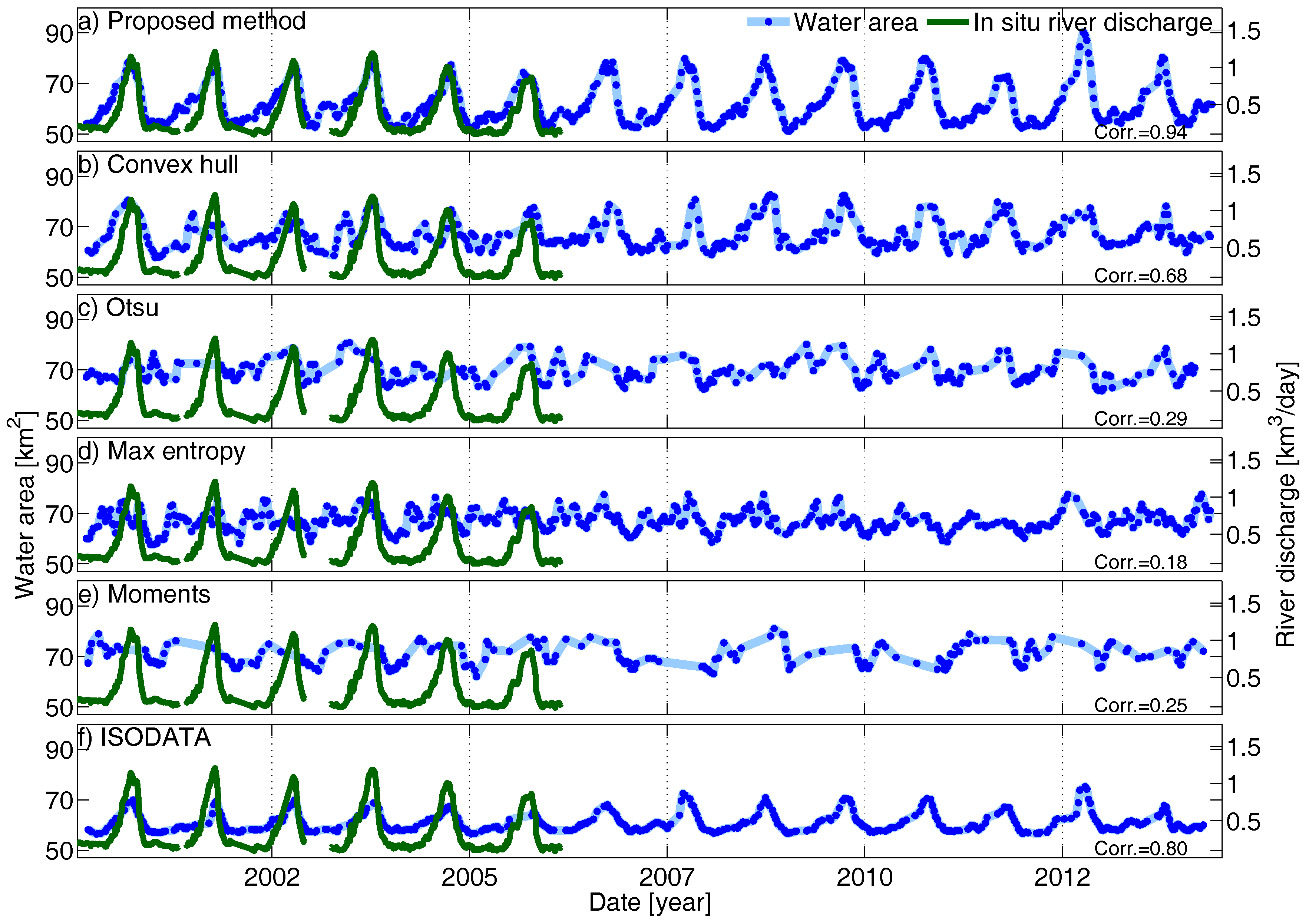
4.4. Comparison with Other Methods

The validation results show the good performance of the proposed method. We now come to the question of whether a simple thresholding method would lead to similar results. To assess this, we compare the performance of different algorithms with our method. We show the results of five different methods: four thresholding algorithms from different groups described in [70], and ISODATA as an unsupervised classification algorithm. We apply these methods on the images of Niger River, Lokaja station (Figure 2c).

• Convex hull thresholding is a method based on shape of the images histogram. After calculating the convex hull of the image histogram, the biggest difference between gray value frequency and convex hull is selected as threshold [71].
• Otsu thresholding is a clustering-based method which assumes that the image contains two bimodal histograms. Then, the optimum threshold is defined in such a way that the variance within the classes is minimized [72].
• Maximum entropy thresholding considers the image as two different sources of data, so when the sum of the two class entropies reaches its maximum. The image is optimally segmented into two classes [73].
• Moments thresholding: in this method, an image is considered as the blurred version of an ideal binary image. Then, the threshold value is defined by matching the first three moments of input image and binary map [74]. This method is considered as an object attribute-based thresholding algorithm.
• ISODATA: as one of the most advanced unsupervised classification methods, ISODATA is selected because of its ability to modify the clusters with respect to the situation of the river [75].

Figure 23. (a–f) Comparison of different classification algorithms on the same data set. Monitoring period: February 2000–September 2014.

Figure 23. (a–f) Comparison of different classification algorithms on the same data set. Monitoring period: February 2000–September 2014.

Figure 23 presents the water area time series generated by applying the aforementioned methods. To assess the performance of the results, we measure the correlation coefficient between water area and in situ river discharge time series. It should be noted that we additionally employed a number of post-classification steps, including a blunder removal step to provide the more accurate water masks. The correlation coefficients indicate that none of the above methods can generate a reliable water mask for hydrological purposes. Among them, ISODATA and convex hull can partially capture the seasonal behavior of the river. Moments and otsu methods cannot estimate the water mask for some images, as they are not able to find a proper threshold because of (1) a huge difference between the number of pixels in each class; (2) the complex relationship between water and land in the river border. By comparing the performance of the proposed method with the others, it is clear that none of the above methods can generate water area time series as accurately as our proposed method (corr. = 0.94). The main reason for the high correlation is that the strong spatial and temporal correlation between pixels is considered in our proposed method.

5. Conclusions and Outlook

We have introduced an automatic water body area monitoring algorithm and applied it to three different river reaches using MODIS images. In this method, a Markov random field (MRF) model was developed to consider all types of available information, including pixel intensity and spatial and temporal interactions between pixels. Then, a maximum a posteriori (MAP) solution for the Bayesian framework was found to determine the most probable water mask. Since the high computational effort of finding a global solution is a serious concern, the problem was reshaped as an energy minimization. To minimize the energy function, we have developed an undirected graph with two terminals and defined the max-flow solution for the graph by augmenting all the possible paths between two terminals. The final residual graph offered the binary water mask representing the MAP solution. A second aim of this study is the uncertainty assessment of derived water masks. Therefore, we computed the confidence level for pixels by measuring the marginal probability of all nodes in the final residual graph.

The time series of the water area together with their uncertainty are generated by applying the method to all images of the given river reaches. The input of our process is a time series of images. The algorithm automatically generates binary and probabilistic water masks together with water area time series, including the uncertainty range. Since cloud-covered images are detected and removed, and since we consider the temporal behavior of the water body, the products are robust against blunders. The algorithm can cope with the effect of sun glint and cloud shadow in the satellite images by considering temporal correlation in the images. Therefore, extra post-processing steps for the final time series are not necessary.

We have employed our method over three river reaches with different channel behavior and different morphology. Two of them are part of the Niger River (near Lokaja and Koulikoro stations), and the third is a river reach containing Malebo Pool along the Congo River near Kinshasa station. Based on the presented results, the method can cover the seasonal change in the river extent and also capture extreme events. The algorithm can successfully extract complex braided river systems and islands in the middle of a river. In our examples, it only fails to extract narrow river branches that are about a pixel wide. We see that, due to the orbit configuration of the both Envisat and SARAL/AltiKa they are not able to measure water level as frequently as water area measured by MODIS. On average, for water area time series, we have 48 values in a year, while at best only 11 water level observations are available. This highlights the advantages of imagery for the characterization of river behaviour in comparison to satellite altimetry.

For the uncertainty estimation, in both water and land masks, pixels with less than 10% marginal probability of their labels were considered as uncertain area. Although the method assigned a label for these pixels, we did not make a firm decision regarding their marginal probability. In the probabilistic water and land masks, most of the pixels with small marginal probabilities were located on shorelines. Considering the coarse MODIS pixel size, most of the pixels located in the river extent were partially covered by water. Therefore, the algorithm cannot assign correct labels for the pixels in this region with high probability. Therefore, we suggest taking advantage of satellite imagery with finer spatial resolution (such as Landsat images) specifically for the uncertain area. In our examples, the magnitude of the uncertain area varies between 8%–23% of the river area, which has a reverse relationship with the water area.

Since ground-truth does not exist, we validate our results indirectly by comparing the obtained water area time series with the in situ river discharge and altimetric water level measurements. In the Niger examples, the high correlation between water area time series and in situ discharge (>0.90) and altimetric water area (>0.80) indicate that we captured the natural behavior of the river reaches, and that our water area estimations are accurate. Correlation was lower in the Congo example because the in situ station is located in an urban area, and the river includes a complex braided system.

In the ideal situation, repeat track altimetry missions can provide a water height measurement for a certain inland water body every ten days. However, by using multiple satellite imag sources, we reach denser time series of water area. The comparison of water level and area time series in our examples reveals that by monitoring the water area, most of the river fluctuations are captured.

We compare the performance of the proposed method with a number of common classification algorithms. By looking at the water area time series and the correlation coefficients between in situ discharge and estimated water area time series, we find that the proposed method can extract the river mask more accurately than the others.

Despite the good performance of our method, its high computational effort is a serious concern in comparison to conventional less accurate pixel-based classifications. Therefore, applying more advanced max-flow algorithms to reduce computational effort can be the next step from this study.Moreover, further study could involve the design of a filter to detect areas with a consistent characteristic over the monitoring period and remove them from the search area by defining their labels in advance.

In this paper, we only considered the sources of information available in satellite images, such as pixel value and spatial and temporal correlations. Fortunately, the structure of MRF gives us the ability to include additional sources of information. Considering different types of information improves the accuracy of water masks. In this way, for future studies, we suggest taking advance of digital terrain models as an auxiliary source of information to extract more accurate dynamic water masks.

The availability of accurate dynamic water masks improves our understanding of surface water variations and helps us to obtain a better overview about the hydrologic cycle. It could be also highly beneficial for hydraulic model calibration. Assimilating the simultaneous measurements of water area and level provides the opportunity to monitor the change in water volume. The availability of accurate river masks can improve the performance of spaceborne water level measurements—especially in narrow rivers. Moreover, the method proposed in this study can help to address the science requirements of the Surface Water and Ocean Topography (SWOT) mission, which will be launched in 2020 [76].

References

- Prigent, C.; Papa, F.; Aires, F.; Rossow, W.; Matthews, E. Global inundation dynamics inferred from multiple satellite observations, 1993–2000. J. Geophys. Res. Atmos. 2007, 112. [Google Scholar] [CrossRef]
- Alsdorf, D.E.; Rodríguez, E.; Lettenmaier, D.P. Measuring surface water from space. Rev. Geophys. 2007, 45. [Google Scholar] [CrossRef]
- Sneeuw, N.; Lorenz, C.; Devaraju, B.; Tourian, M.J.; Riegger, J.; Kunstmann, H.; Bárdossy, A. Estimating runoff using hydro-geodetic approaches. Surv. Geophys. 2014, 35, 1333–1359. [Google Scholar] [CrossRef]
- Zhang, G.; Yao, T.; Xie, H.; Zhang, K.; Zhu, F. Lakes’ state and abundance across the Tibetan Plateau. Chin. Sci. Bull. 2014, 59, 3010–3021. [Google Scholar] [CrossRef]
- Liu, G.; Schwartz, F.W.; Tseng, K.H.; Shum, C. Discharge and water-depth estimates for ungauged rivers: Combining hydrologic, hydraulic, and inverse modeling with stage and water-area measurements from satellites. Water Resour. Res. 2015, 51, 6017–6035. [Google Scholar] [CrossRef]
- Zhang, G.; Xie, H.; Kang, S.; Yi, D.; Ackley, S.F. Monitoring lake level changes on the Tibetan Plateau using ICESat altimetry data (2003–2009). Remote Sens. Environ. 2011, 115, 1733–1742. [Google Scholar] [CrossRef]
- Li, C.H.; Lee, C.K. Minimum cross entropy thresholding. Pattern Recognit. 1993, 26, 617–625. [Google Scholar] [CrossRef]
- Lu, D.; Mausel, P.; Brondizio, E.; Moran, E. Change detection techniques. Int. J. Remote Sens. 2004, 25, 2365–2401. [Google Scholar] [CrossRef]
- Sandholt, I.; Nyborg, L.; Fog, B.; Lô, M.; Bocoum, O.; Rasmussen, K. Remote sensing techniques for flood monitoring in the Senegal River Valley. Geogr. Tidsskr. Dan. J. Geogr. 2003, 103, 71–81. [Google Scholar] [CrossRef]
- Bonn, F.; Dixon, R. Monitoring flood extent and forecasting excess runoff risk with RADARSAT-1 data. Nat. Hazards 2005, 35, 377–393. [Google Scholar] [CrossRef]
- Martinis, S.; Twele, A.; Strobl, C.; Kersten, J.; Stein, E. A Multi-Scale Flood Monitoring System Based on Fully Automatic MODIS and TerraSAR-X Processing Chains. Remote Sens. 2013, 5, 5598–5619. [Google Scholar] [CrossRef]
- Garay, M.J.; Diner, D.J. Multi-angle Imaging SpectroRadiometer (MISR) time-lapse imagery of tsunami waves from the 26 December 2004 Sumatra-Andaman earthquake. Remote Sens. Environ. 2007, 107, 256–263. [Google Scholar] [CrossRef]
- Munyati, C. Use of principal component analysis (PCA) of remote sensing images in wetland change detection on the Kafue Flats, Zambia. Geocarto Int. 2004, 19, 11–22. [Google Scholar] [CrossRef]
- Wang, Y. Seasonal change in the extent of inundation on floodplains detected by JERS-1 Synthetic Aperture Radar data. Int. J. Remote Sens. 2004, 25, 2497–2508. [Google Scholar] [CrossRef]
- Feyisa, G.L.; Meilby, H.; Fensholt, R.; Proud, S.R. Automated Water Extraction Index: A new technique for surface water mapping using Landsat imagery. Remote Sens. Environ. 2014, 140, 23–35. [Google Scholar] [CrossRef]
- Ryu, J.H.; Won, J.S.; Min, K.D. Waterline extraction from Landsat TM data in a tidal flat: A case study in Gomso Bay, Korea. Remote Sens. Environ. 2002, 83, 442–456. [Google Scholar] [CrossRef]
- Kuenzer, C.; Guo, H.; Huth, J.; Leinenkugel, P.; Li, X.; Dech, S. Flood Mapping and Flood Dynamics of the Mekong Delta: ENVISAT-ASAR-WSM Based Time Series Analyses. Remote Sens. 2013, 5, 687–715. [Google Scholar] [CrossRef] [Green Version]
- Kuenzer, C.; Klein, I.; Ullmann, T.; Georgiou, E.F.; Baumhauer, R.; Dech, S. Remote sensing of river delta inundation: Exploiting the potential of coarse spatial resolution, temporally-dense MODIS Time Series. Remote Sens. 2015, 7, 8516–8542. [Google Scholar] [CrossRef]
- Gao, H.; Birkett, C.; Lettenmaier, D.P. Global monitoring of large reservoir storage from satellite remote sensing. Water Resour. Res. 2012, 48. [Google Scholar] [CrossRef]
- Tourian, M.; Elmi, O.; Chen, Q.; Devaraju, B.; Roohi, S.; Sneeuw, N. A spaceborne multisensor approach to monitor the desiccation of Lake Urmia in Iran. Remote Sens. Environ. 2015, 156, 349–360. [Google Scholar] [CrossRef]
- Klein, I.; Dietz, A.J.; Gessner, U.; Galayeva, A.; Myrzakhmetov, A.; Kuenzer, C. Evaluation of seasonal water body extents in Central Asia over the past 27 years derived from medium-resolution remote sensing data. Int. J. Appl. Earth Obs. Geoinf. 2014, 26, 335–349. [Google Scholar] [CrossRef]
- Doña, C.; Chang, N.B.; Caselles, V.; Sánchez, J.M.; Pérez-Planells, L.; Bisquert, M.D.M.; García-Santos, V.; Imen, S.; Camacho, A. Monitoring Hydrological Patterns of Temporary Lakes Using Remote Sensing and Machine Learning Models: Case Study of La Mancha Húmeda Biosphere Reserve in Central Spain. Remote Sens. 2016, 8, 618. [Google Scholar] [CrossRef]
- Carroll, M.; Wooten, M.; DiMiceli, C.; Sohlberg, R.; Kelly, M. Quantifying Surface Water Dynamics at 30 Meter Spatial Resolution in the North American High Northern Latitudes 1991–2011. Remote Sens. 2016, 8, 622. [Google Scholar] [CrossRef]
- Huang, C.; Chen, Y.; Zhang, S.; Li, L.; Shi, K.; Liu, R. Surface Water Mapping from Suomi NPP-VIIRS Imagery at 30 m Resolution via Blending with Landsat Data. Remote Sens. 2016, 8, 631. [Google Scholar] [CrossRef]
- McFeeters, S.K. Using the Normalized Difference Water Index (NDWI) within a Geographic Information System to Detect Swimming Pools for Mosquito Abatement: A Practical Approach. Remote Sens. 2013, 5, 3544–3561. [Google Scholar] [CrossRef]
- Kallio, K.; Attila, J.; Härmä, P.; Koponen, S.; Pulliainen, J.; Hyytiäinen, U.M.; Pyhälahti, T. Landsat ETM+ images in the estimation of seasonal lake water quality in boreal river basins. Environ. Manag. 2008, 42, 511–522. [Google Scholar] [CrossRef] [PubMed]
- Fisher, A.; Danaher, T. A Water Index for SPOT5 HRG Satellite Imagery, New South Wales, Australia, Determined by Linear Discriminant Analysis. Remote Sens. 2013, 5, 5907–5925. [Google Scholar] [CrossRef]
- Elmi, O. The Role of Multispectral Image Transformations in Change Detection. Master’s Thesis, University of Stuttgart, Stuttgart, Germany, 2015. [Google Scholar]
- Wohlfart, C.; Liu, G.; Huang, C.; Kuenzer, C. A River Basin over the Course of Time: Multi-Temporal Analyses of Land Surface Dynamics in the Yellow River Basin (China) Based on Medium Resolution Remote Sensing Data. Remote Sens. 2016, 8, 186. [Google Scholar] [CrossRef]
- Tourian, M.; Tarpanelli, A.; Elmi, O.; Qin, T.; Brocca, L.; Moramarco, T.; Sneeuw, N. Spatiotemporal densification of river water level time series by multimission satellite altimetry. Water Resour. Res. 2016. [Google Scholar] [CrossRef]
- Elmi, O.; Tourian, M.J.; Sneeuw, N. River discharge estimation using channel width from satellite imagery. In Proceedings of the 2015 IEEE International Geoscience and Remote Sensing Symposium (IGARSS), Milan, Italy, 26–31 July 2015; pp. 727–730.
- Pavelsky, T.M. Using width-based rating curves from spatially discontinuous satellite imagery to monitor river discharge. Hydrol. Process. 2014, 28, 3035–3040. [Google Scholar] [CrossRef]
- Townsend, P.A. Mapping seasonal flooding in forested wetlands using multi-temporal Radarsat SAR. Photogram. Eng. Remote Sens. 2001, 67, 857–864. [Google Scholar]
- Brivio, P.A.; Colombo, R.; Maggi, M.; Tomasoni, R. Integration of remote sensing data and GIS for accurate mapping of flooded areas. Int. J. Remote Sens. 2002, 23, 429–441. [Google Scholar] [CrossRef]
- Cao, W. Change Detection Using SAR Data. Master’s Thesis, University of Stuttgart, Stuttgart, Germany, 2013. [Google Scholar]
- Weih, R.C., Jr.; Riggan, N.D., Jr. Object-based classification vs. pixel-based classification: Comparative importance of multi-resolution imagery. In Proceedings of the GEOBIA 2010: Geographic Object-Based Image Analysis, Ghent, Belgium, 29 June–2 July 2010; Volume 38, p. 6.
- Hogan, C.M. Niger River; McGinley, M., Ed.; National Council for Science and Environment: Washington, DC, USA, 2013. [Google Scholar]
- Cretaux, J.F.; Berge-Nguyen, M.; Leblanc, M.; Abarca Del Rio, R.; Delclaux, F.; Mognard, N.; Lion, C.; Pandey, R.K.; Tweed, S.; Calmant, S.; et al. Flood mapping inferred from remote sensing data. Int. Water Technol. J. 2011, 1, 48–62. [Google Scholar]
- O’Loughlin, F.; Trigg, M.; Schumann, G.P.; Bates, P. Hydraulic characterization of the middle reach of the Congo River. Water Resour. Res. 2013, 49, 5059–5070. [Google Scholar] [CrossRef]
- Da Silva, J.S.; Calmant, S.; Seyler, F.; Filho, O.C.R.; Cochonneau, G.; Mansur, W.J. Water levels in the Amazon basin derived from the ERS 2 and ENVISAT radar altimetry missions. Remote Sens. Environ. 2010, 114, 2160–2181. [Google Scholar] [CrossRef]
- Tourian, M.; Sneeuw, N.; Bárdossy, A. A quantile function approach to discharge estimation from satellite altimetry (ENVISAT). Water Resour. Res. 2013, 49, 4174–4186. [Google Scholar] [CrossRef]
- Veksler, O. Efficient Graph-Based Energy Minimization Methods in Computer Vision. Ph.D. Thesis, Cornell University, Ithaca, NY, USA, 1999. [Google Scholar]
- Geman, S.; Geman, D. Stochastic relaxation, Gibbs distributions, and the Bayesian restoration of images. IEEE Trans. Pattern Anal. Mach. Intell. 1984, PAMI-6, 721–741. [Google Scholar] [CrossRef]
- Ishikawa, H.; Geiger, D. Segmentation by grouping junctions. In Proceedings of the IEEE Conference on Computer Vision and Pattern Recognition, Santa Barbara, CA, USA, 25 June 1998; pp. 125–131.
- Couprie, C.; Grady, L.; Najman, L.; Talbot, H. Power watershed: A unifying graph-based optimization framework. IEEE Trans. Pattern Anal. Mach. Intell. 2011, 33, 1384–1399. [Google Scholar] [CrossRef] [PubMed] [Green Version]
- Boykov, Y.; Veksler, O.; Zabih, R. Markov random fields with efficient approximations. In Proceedings of the IEEE Conference on Computer Vision and Pattern Recognition, Santa Barbara, CA, USA, 25 June 1998; pp. 648–655.
- Boykov, Y.; Veksler, O.; Zabih, R. Fast approximate energy minimization via graph cuts. IEEE Trans. Pattern Anal. Mach. Intell. 2001, 23, 1222–1239. [Google Scholar] [CrossRef]
- Bruzzone, L.; Prieto, D.F. An adaptive semiparametric and context-based approach to unsupervised change detection in multitemporal remote-sensing images. IEEE Trans. Image Process. 2002, 11, 452–466. [Google Scholar] [CrossRef] [PubMed]
- Mota, G.L.; Feitosa, R.Q.; Coutinho, H.L.; Liedtke, C.E.; Müller, S.; Pakzad, K.; Meirelles, M.S. Multitemporal fuzzy classification model based on class transition possibilities. ISPRS J. Photogram. Remote Sens. 2007, 62, 186–200. [Google Scholar] [CrossRef]
- Solberg, A.H.S.; Taxt, T.; Jain, A.K. A Markov random field model for classification of multisource satellite imagery. IEEE Trans. Geosci. Remote Sens. 1996, 34, 100–113. [Google Scholar] [CrossRef]
- Martinis, S.; Twele, A. A hierarchical spatio-temporal Markov model for improved flood mapping using multi-temporal X-band SAR data. Remote Sens. 2010, 2, 2240–2258. [Google Scholar] [CrossRef]
- Besag, J. On the statistical analysis of dirty pictures. J. R. Stat. Soc. Ser. B (Methodol.) 1986, 48, 259–302. [Google Scholar] [CrossRef]
- Szeliski, R.; Zabih, R.; Scharstein, D.; Veksler, O.; Kolmogorov, V.; Agarwala, A.; Tappen, M.; Rother, C. A comparative study of energy minimization methods for markov random fields. In European Conference on Computer Vision; Springer: Berlin/Heidelberg, Germany, 2006; pp. 16–29. [Google Scholar]
- Greig, D.; Porteous, B.; Seheult, A.H. Exact maximum a posteriori estimation for binary images. J. R. Stat. Soc. Ser. B 1989, 51, 271–279. [Google Scholar]
- Boykov, Y.; Kolmogorov, V. An experimental comparison of min-cut/max-flow algorithms for energy minimization in vision. IEEE Trans. Pattern Anal. Mach. Intell. 2004, 26, 1124–1137. [Google Scholar] [CrossRef] [PubMed]
- Goldberg, A.V.; Hed, S.; Kaplan, H.; Tarjan, R.E.; Werneck, R.F. Maximum flows by incremental breadth-first search. In Algorithms–ESA 2011; Springer: Berlin/Heidelberg, Germany, 2011; pp. 457–468. [Google Scholar]
- Veksler, O. Image segmentation by nested cuts. IEEE Conf. Comput. Vis. Pattern Recognit. 2000, 1, 339–344. [Google Scholar]
- Kolmogorov, V.; Zabin, R. What energy functions can be minimized via graph cuts? IEEE Trans. Pattern Anal. Mach. Intell. 2004, 26, 147–159. [Google Scholar] [CrossRef] [PubMed]
- Kohli, P.; Torr, P. Measuring uncertainty in graph cut solutions-efficiently computing min-marginal energies using dynamic graph cuts. In Proceedings of the 9th European Conference on Computer Vision, Graz, Austria, 7–13 May 2006; pp. 30–43.
- Boykov, Y.Y.; Jolly, M.P. Interactive graph cuts for optimal boundary & region segmentation of objects in ND images. In Proceedings of the Eighth IEEE International Conference on Computer Vision (ICCV 2001), Vancouver, BC, Canada, 7–14 July 2001; Volume 1, pp. 105–112.
- Besag, J. Spatial interaction and the statistical analysis of lattice systems. J. R. Stat. Soc. Ser. B (Methodol.) 1974, 36, 192–236. [Google Scholar]
- Boykov, Y.; Veksler, O. Graph cuts in vision and graphics: Theories and applications. In Handbook of Mathematical Models in Computer Vision; Springer: Berlin/Heidelberg, Germany, 2006; pp. 79–96. [Google Scholar]
- Li, S.Z. Markov Random Field Modeling in Image Analysis; Springer: Berlin/Heidelberg, Germany, 2009. [Google Scholar]
- Ford, L.; Fulkerson, D.R. Flows in Networks; Princeton University Press: Princeton, NJ, USA, 1962. [Google Scholar]
- Goldberg, A.V.; Tarjan, R.E. A new approach to the maximum-flow problem. J. ACM 1988, 35, 921–940. [Google Scholar] [CrossRef]
- Dinits, E. Algorithm of solution to problem of maximum flow in network with power estimates. Dokl. Akad. Nauk SSSR 1970, 11, 1277–1280. [Google Scholar]
- Kohli, P.; Torr, P.H. Measuring uncertainty in graph cut solutions. Comput. Vis. Image Underst. 2008, 112, 30–38. [Google Scholar] [CrossRef]
- Tarlow, D.; Adams, R.P. Revisiting uncertainty in graph cut solutions. In Proceedings of the 2012 IEEE Conference on Computer Vision and Pattern Recognition (CVPR), Providence, RI, USA, 16–21 June 2012; pp. 2440–2447.
- Leopold, L.B.; Maddock, T., Jr. The Hydraulic Geometry of Stream Channels and Some Physiographic Implications; US Geological Survey Professional Paper No. 252; Superintendent of Documents; U.S. Government Printing Office: Washington, DC, USA, 1953.
- Sezgin, M.; Sankur, B. Survey over image thresholding techniques and quantitative performance evaluation. J. Electron. Imaging 2004, 13, 146–168. [Google Scholar]
- Rosenfeld, A.; de La Torre, P. Histogram concavity analysis as an aid in threshold selection. IEEE Trans. Syst. Man Cybern. 1983, SMC-13, 231–235. [Google Scholar] [CrossRef]
- Otsu, N. A threshold selection method from gray-level histograms. Automatica 1975, 11, 23–27. [Google Scholar] [CrossRef]
- Glasbey, C.A. An analysis of histogram-based thresholding algorithms. CVGIP Graph. Models Image Process. 1993, 55, 532–537. [Google Scholar] [CrossRef]
- Tsai, W.H. Moment-preserving thresolding: A new approach. Comput. Vis. Graph. Image Process. 1985, 29, 377–393. [Google Scholar] [CrossRef]
- Ball, G.H.; Hall, D.J. ISODATA, A Novel Method of Data Analysis and Pattern Classification; Technical Report; DTIC Document: Fort Belvoir, VA, USA, 1965. [Google Scholar]
- Biancamaria, S.; Lettenmaier, D.P.; Pavelsky, T.M. The SWOT mission and its capabilities for land hydrology. Surv. Geophys. 2016, 37, 307–337. [Google Scholar] [CrossRef]