Article

Frozen: The Potential and Pitfalls of Ground-Penetrating Radar for Archaeology in the Alaskan Arctic

1
Cornell Tree Ring Laboratory, Department of Classics and Cornell Institute of Archaeology and Material Studies, Cornell University, Ithaca, NY 14853, USA
2
U.S. National Park Service, Gates of the Arctic National Park and Preserve, Yukon-Charley Rivers National Preserve, Fairbanks, AK 99709, USA
3
Histoire de l'Art et Archéologie, Paris 1 Pantheon Sorbonne University, Paris 75005, France
4
Department of Anthropology and Circumpolar Laboratory, Brown University, Providence, RI 02912, USA
5
Institute for Arctic and Alpine Research, University of Colorado, Boulder, CO 80309, USA
6
U.S. National Park Service, Alaska Regional Office, Anchorage, AK 99501, USA
7
Department of Anthropology, University at Albany, Albany, NY 12222, USA
*
Author to whom correspondence should be addressed.
Remote Sens. 2016, 8(12), 1007; https://doi.org/10.3390/rs8121007
Submission received: 28 September 2016 / Revised: 26 November 2016 / Accepted: 1 December 2016 / Published: 9 December 2016
(This article belongs to the Special Issue Archaeological Prospecting and Remote Sensing)

Abstract

:
Ground-penetrating radar (GPR) offers many advantages for assessing archaeological potential in frozen and partially frozen contexts in high latitude and alpine regions. These settings pose several challenges for GPR, including extreme velocity changes at the interface of frozen and active layers, cryogenic patterns resulting in anomalies that can easily be mistaken for cultural features, and the difficulty in accessing sites and deploying equipment in remote settings. In this study we discuss some of these challenges while highlighting the potential for this method by describing recent successful investigations with GPR in the region. We draw on cases from Bering Land Bridge National Preserve, Cape Krusenstern National Monument, Kobuk Valley National Park, and Gates of the Arctic National Park and Preserve. The sites required small aircraft accessibility with light equipment loads and minimal personnel. The substrates we investigate include coastal saturated active layer over permafrost, interior well-drained active layer over permafrost, a frozen thermo-karst lake, and an alpine ice patch. These examples demonstrate that GPR is effective at mapping semi-subterranean house remains in several contexts, including houses with no surface manifestation. GPR is also shown to be effective at mapping anomalies from the skeletal remains of a late Pleistocene mammoth frozen in ice. The potential for using GPR in ice and snow patch archaeology, an area of increasing interest with global environmental change exposing new material each year, is also demonstrated.

Graphical Abstract

1. Introduction

Geophysical methods were first tested at archaeological sites in Alaska by J.L. Giddings and D.D. Anderson in 1960. These early investigations with proton precession magnetometry and electrical resistivity were wrought with challenges, and the methods were abandoned after one season of trials [1]. Many improvements have been made in geophysical technology since the early investigations of Giddings and Anderson. Multiple geophysical methods, including ground-penetrating radar (GPR), have now been successfully used for archaeological investigations in Alaska [2,3,4]; however, Arctic settings in the region are still fraught with challenges for geophysical investigations. Here we describe some recent applications of ground-penetrating radar in higher latitude regions of Alaska, highlighting the extraordinary potential of the method for site reconnaissance in a variety of environmental settings, while also describing some common pitfalls of GPR in such places.
We draw on examples from multiple locations managed by the U.S. National Park Service (Figure 1). At Cape Krusenstern National Monument, GPR revealed complex patterned ground created by the freeze-thaw cycle at the Old Whaling beach ridge [3], while multi-year GPR data collected at this location illustrates temporal variations in the permafrost table. In Kobuk Valley National Park, a GPR investigation of an early contact period Inupiat settlement revealed an earlier, deeper occupation in the permafrost just beneath the known site. At the Cape Espenberg locality in Bering Land Bridge National Preserve, a deep Birnirk period house complex was investigated with GPR, with shallower portions in the saturated active layer and deeper portions frozen in permafrost. Also at Bering Land Bridge National Preserve, the skeletal remains of a late Pleistocene mammoth embedded in the bottom of a thermokarst lake were successfully mapped from the surface of the frozen lake. Finally, in Gates of the Arctic National Park and Preserve an alpine ice patch was mapped with GPR, showing clear bedding and suspended anomalies. In similar ice patch settings elsewhere in the region, ancient hunters targeted caribou and occasionally lost weaponry and other tools that have long been preserved in frozen conditions. With such features now melting, artifacts of these hunters are being revealed, often in association with deposits of caribou dung that might be potentially identified with GPR before the deposits melt. This latter case lays the groundwork for how GPR may be integrated into such investigations, and contribute to the management of invaluable cultural resources, particularly those that face the threat of environmental change.

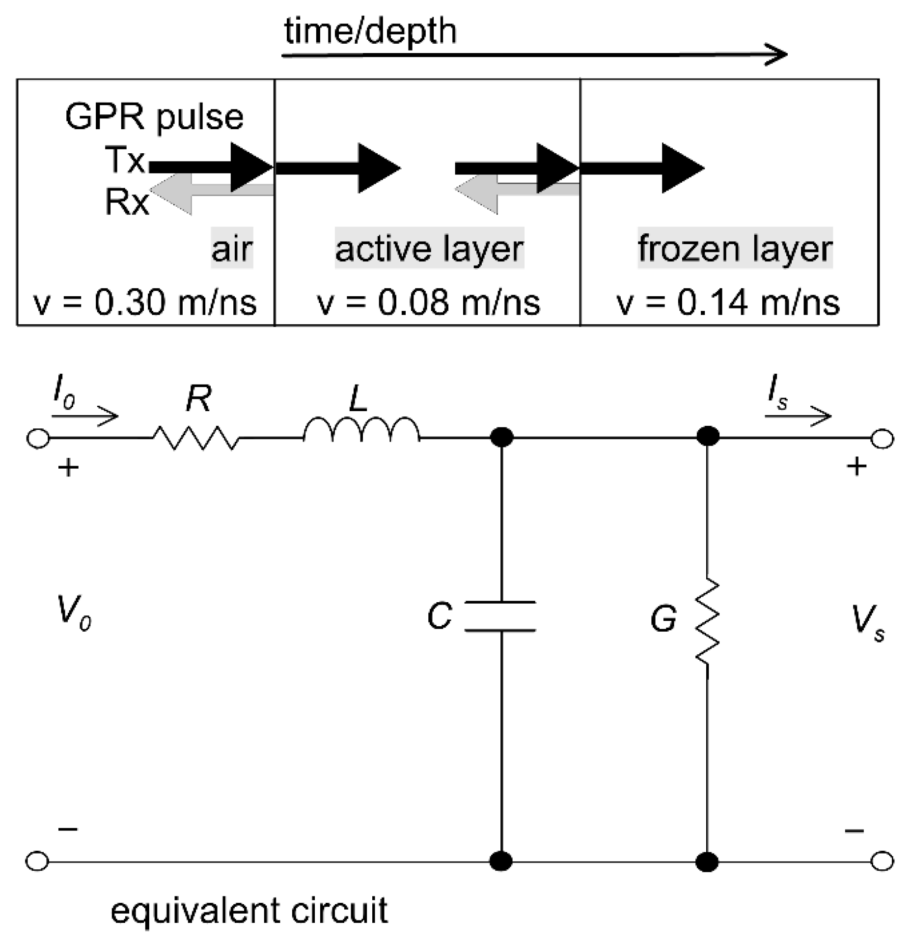
Ground-Penetrating Radar (GPR) in Frozen and Partially Frozen Media

Sub-surface velocity is the most crucial parameter to determine when applying GPR to archaeological investigations, since accurate estimation of depth and dimensions of archaeological features is contingent upon the accuracy of velocity estimates [5]. This is of great concern in Arctic settings where velocities may abruptly change with a shift from thawed to frozen media. A review of frequently used methods for estimating GPR velocity can be found in [5,6,7]. Case studies in this paper relied primarily on the technique of hyperbola fitting to estimate velocity. When a GPR profile is collected perpendicular to a point-scatter (i.e., an anomaly in the ground that results in a diffraction hyperbola) velocity may be estimated from the resulting hyperbolic curve on the basis of increasing travel time associated with increasing path length with regard to horizontal distance from the sub-surface anomaly [8,9]. The relationship of antenna position x, point-scatter depth d, travel time T, velocity v, and T 0 (the time at which the antenna is directly above the point-scatterer) can be described in simple terms by (Equation (1))
T = ( 4 x 2 v 2 + T 0 2 ) 1 2
where
T 0 = 2 d v
A hyperbola fitting method may be used to match the spread of the observed hyperbola tails to those of calculated hyperbolas for a range of velocities and is undertaken as part of the post-processing of GPR data [10].
Accurate velocity estimates are especially important in partially frozen settings where velocities often approach extremes (Table 1). This is due to the abrupt contrast in relative electrical permittivity ε r between frozen and wet material, as ε r in most instances (within the frequency range used for GPR and normally encountered ranges of electrical conductivity) will be the primary property controlling velocity, and is itself controlled by liquid water content. The relationship in the simplest case can be described by (Equation (2)), where C is the speed of light.
ε r = ( C v ) 2
This disparity in electrical properties between thawed active layer and permafrost has previously been described in Alaskan contexts [11]. While a fully frozen medium results in a fast, though uniform velocity, the partially frozen medium often results in extreme velocity shifts between frozen and active layers (the portion of the ground which thaws seasonally). Determining the accurate depth and dimensions of an archaeological feature in such a case requires an accurate estimate of velocity in the substrate in which the feature of interest occurs (i.e., active layer or frozen layer). Of course archaeological features may cross this boundary and rest partially in a frozen layer and partially in the active layer. Another consideration of the partially frozen medium is that the active layer may be saturated with water and will therefore exhibit a very slow velocity. Since water cannot infiltrate vertically when underlain by a frozen layer, it often remains perched upon that layer. Velocities as slow as 0.05 m/ns might occur in such situations. If features in both the active layer and the frozen layer are to be assessed (or if features straddle the vertical boundary of these layers), the permafrost interface must be identified, and the two layers must be given separate velocity estimates and separate processing. Not doing so could result in distorted estimates of depths and dimensions. Further, it must be kept in mind that energy returned from within the permafrost layer has passed through the active layer twice. For this reason, estimating the velocity from a table (e.g., Table 1) can be inaccurate, as the average velocity must also account for transmission through the active layer, which is why an empirical method for determining average velocity is best. For the examples used in this paper, hyperbola fitting was undertaken using the spread of hyperbolic curves to estimate the average velocity (of the total ground from surface to a particular depth) for purposes of both depth determination and migration. When the estimate is correct, the majority of hyperbola tails will be eliminated in the post-migration data for the layer of interest. Even so, all methods for estimating velocity have shortcomings and limitations [5], so when possible, direct checks of depth estimates by comparing to excavation, cores, scarps etc. to correlate known interfaces with those detected by GPR is advisable. In the case studies presented here, observed depths from excavation have been used as a check on velocity/depth estimates yielded from GPR results. Depth estimates were found to be consistent with excavated cases.
A transmission line model, adapted from Heaviside’s telegrapher’s equations (1880) can illustrate a GPR pulse through a multi-velocity medium. This can be represented schematically as an equivalent circuit diagram (Figure 2). In this instance, the GPR pulse propagation is analogous to electrical voltage propagation where V is voltage, I is current in amperes, R = resistance per unit length in Ohm/m, L = inductance per unit length in Henry/m, C = capacitance per unit length in Farads/m, G = conductance per unit length in Seimens/m. The observed case can be more complicated due to intermittent ice, perched water at the permafrost interface, and textural variations within the active layer, factors which also complicate velocity estimates.

2. Methods

The instrument used for all examples described in this paper was a 250 MHz center frequency (band width 125–375 MHz) Noggin System by Sensors and Software Inc. Instrument, and survey parameters are listed in Table 2. All sites used as examples in this paper required access by small aircraft, including float planes, ski planes and helicopters (Figure 3). This, in turn, required light equipment loads, which in some cases had to be backpacked some distance to and from a suitable landing site. This situation made options such as push-cart GPR setups and multiple antenna arrays less desirable. For this reason, a mid-range antenna frequency (i.e., one that can be trusted for a balance of both reasonable resolution and penetration) and small sled deployment setup were chosen for the work (Figure 3).
Data processing procedures included: visual inspection and editing of data, time-zero re-picking, dewow, velocity estimation with hyperbola matching, SEC-2 gain, background subtraction (avg. of all traces); migration (where indicated); envelope (where indicated); time-depth conversion; and topographic corrections (when necessary). In some instances, a running average (three-trace window) was applied as a horizontal low pass filter to emphasize the interface of the frozen and active layers. Data processing was undertaken with EKKOProject by Sensors and Software Inc. and final images were produced with Voxler 4 and/or Surfer 13, both by Golden Software Inc. Final figures include profiles (vertical cross-section), time-depth slices (plan-view) and 3-D perspective view images using partially opaque data volumes and/or fence diagrams.

3. Results and Discussion

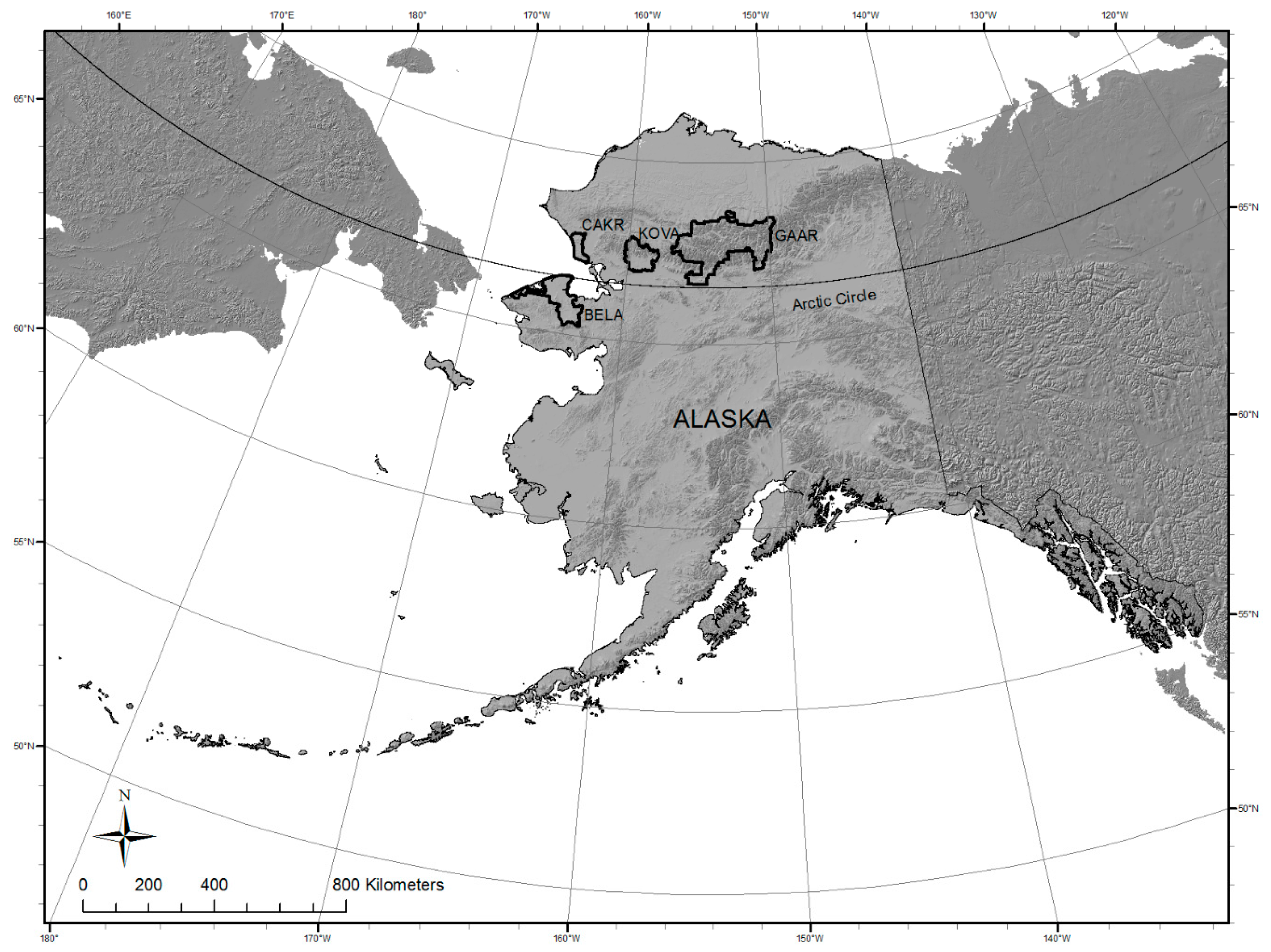
3.1. Dynamics of the Partially Frozen Environment: The Old Whaling Ridge at Cape Krusenstern National Monument

3.1.1. The Old Whaling Site

In the mid-twentieth century, J. Louis Giddings and his students documented two groups of prehistoric house features dating to ca. 3000 BP. These were located on an ancient beach ridge in what is now Cape Krusenstern National Monument in northwestern Alaska (Figure 1), and they were noteworthy because they contained a unique artifact assemblage and house forms unlike any other site yet (or since) discovered in Alaska. The site also contained whale bones, and large weapon heads and butchering tools, which Giddings interpreted as evidence for active whale hunting by the inhabitants, and the basis for what he named the “Old Whaling” culture [15]. Based on the different construction techniques between the various house features, Giddings believed that the site contained evidence of both cold and warm season occupations by the same cultural group [15,16]. Other researchers have since highlighted similarities between the Old Whaling site and maritime cultures evident in the Bering Strait region, primarily in Chukotka [17,18]. Others have suggested connections to the widespread and comparatively well-known Northern Archaic tradition [19,20]. Renewed test excavations at the site in 2003 found additional buried deposits suggesting the history of occupations was more complex than previously envisioned [19,21].

3.1.2. GPR Investigations at the Old Whaling Site, 2011–2016

The Old Whaling site lies on beach ridge 53, roughly 1.3 km from the coast. There is a 100 m strip of open space between two discrete clusters of earthen houses—Giddings’s summer and winter settlements [15,16]. A 2011 GPR survey of this open space drew attention to the freeze-thaw dynamics of the site [3] and added concern over the general threat of permafrost variations, leading to subsequent data collection over the next five years for the purpose of monitoring these dynamics in relation to global environmental change. The resulting data offer a glimpse of how this type of environment varies throughout the summer and from year to year from a GPR perspective.
As average temperatures rise above freezing in May, the frozen ground begins to thaw. By the end of summer, this thawed layer (active layer) has reached its maximum thickness. In early fall, as average temperatures drop below freezing, the thawed ground begins to freeze once again. The interface between the active and frozen layers is detectable with GPR, and leads to predicable velocity changes (Figure 4). By late August, the thickness of the active layer may be double what is observed in June or July (Figure 5). Because this layer thaws and re-freezes while often exhibiting a significant water content, networks of distinct patterns form in the sub-surface that are visible in GPR data (Figure 6), a phenomenon occasionally observed on the surface of some areas underlain by permafrost [22]. Similar features have been mapped with GPR at other locations in Alaska [23,24]. Many components of these patterns, if viewed in isolation, could easily be mistaken for house perimeters on the basis of size and shape. Since these patterns appear as broad networks, they do not exhibit the detail of internal house structure (hearths, floors etc.) and most often continue unchanged for the full depth range of the active layer (while houses would vary much more with depth); these are thus readily distinguishable from most cultural features observed in GPR data.

3.2. Semi-Subterranean Houses in Partially Frozen Settings: Bering Land Bridge National Preserve and Kobuk Valley National Park

Houses throughout most of the occupational history of Alaska were semi-subterranean structures of wood and earth (sometimes bone). Though such structures varied in size and complexity, they generally included a wood-framed depression, often with an entry tunnel and sometimes a central hearth. A general diagram of such a house is shown in Figure 6. The archaeological remains of such a structure may, at various times of year, be fully or partially frozen, often straddling thawed and frozen layers. In this section, we give examples from two sites where house features occur both in thawed and frozen ground.

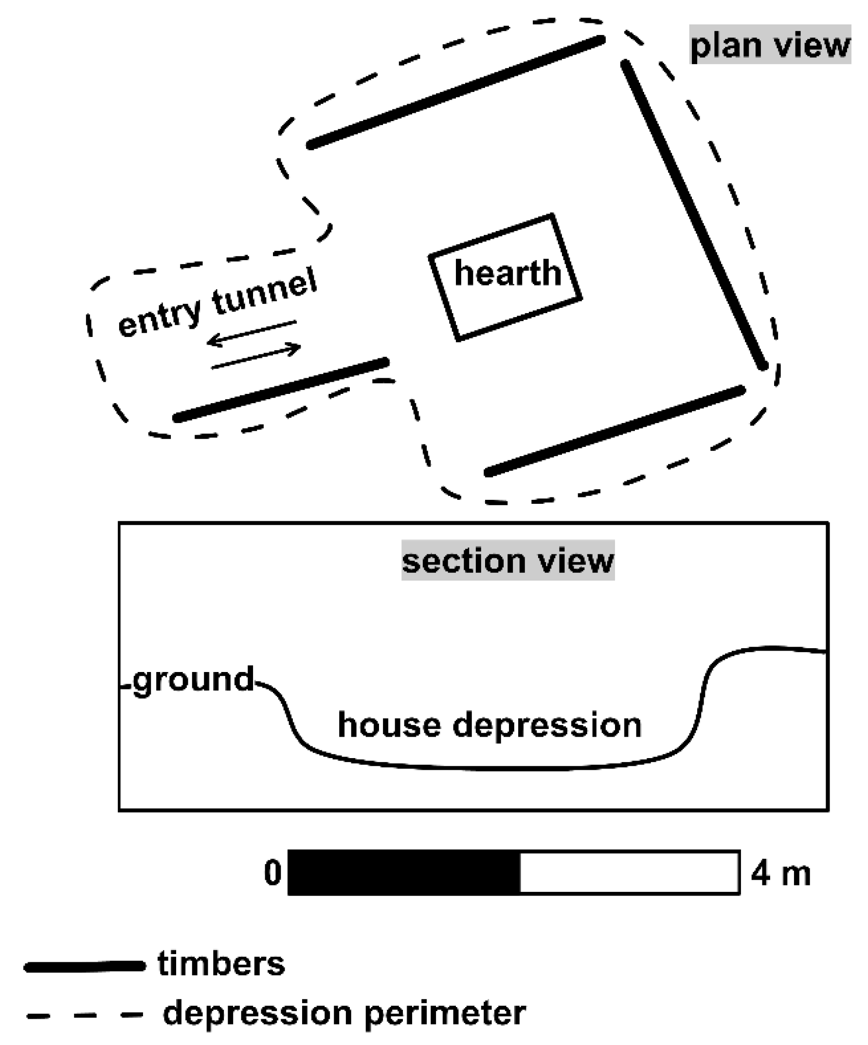
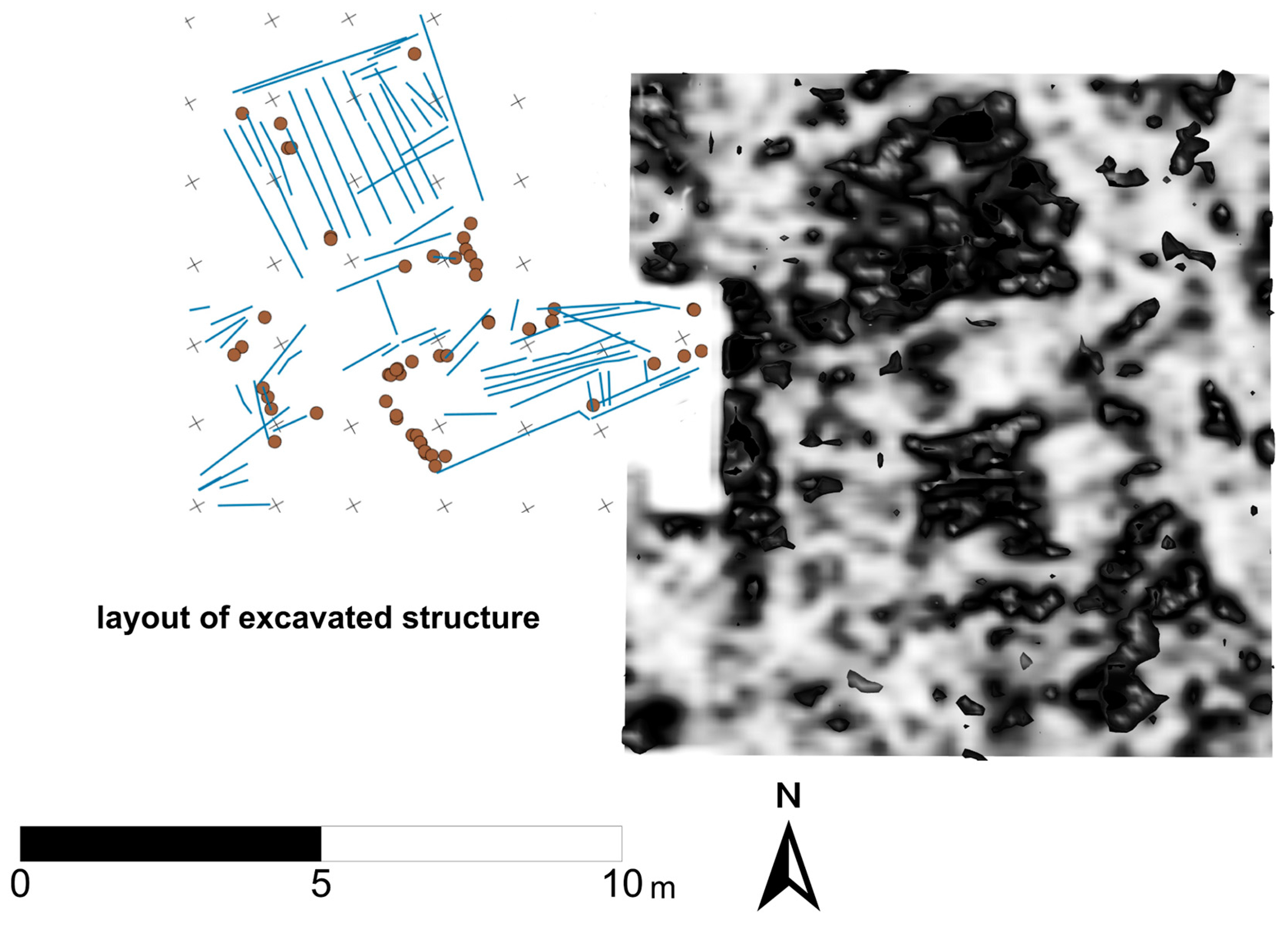
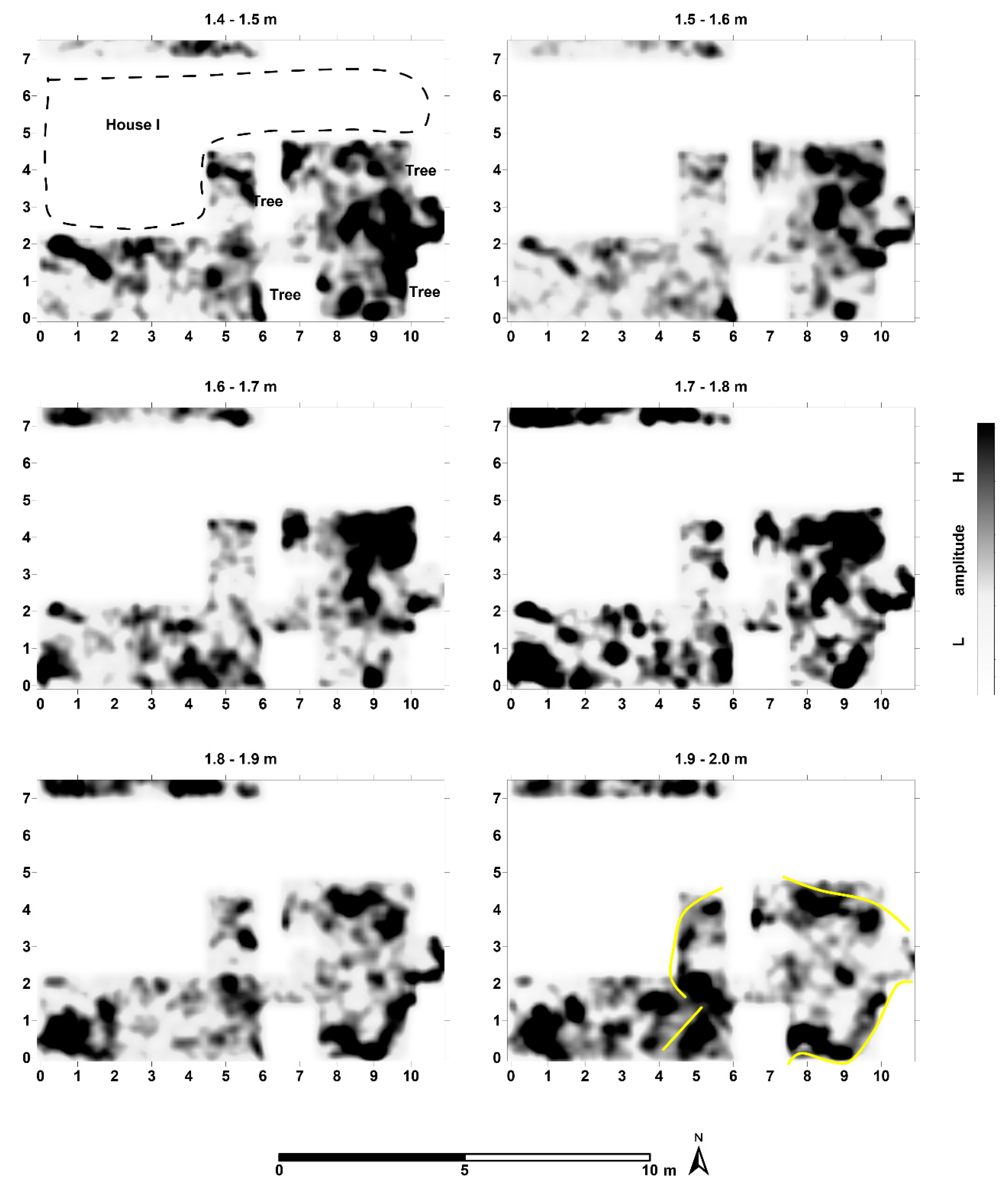
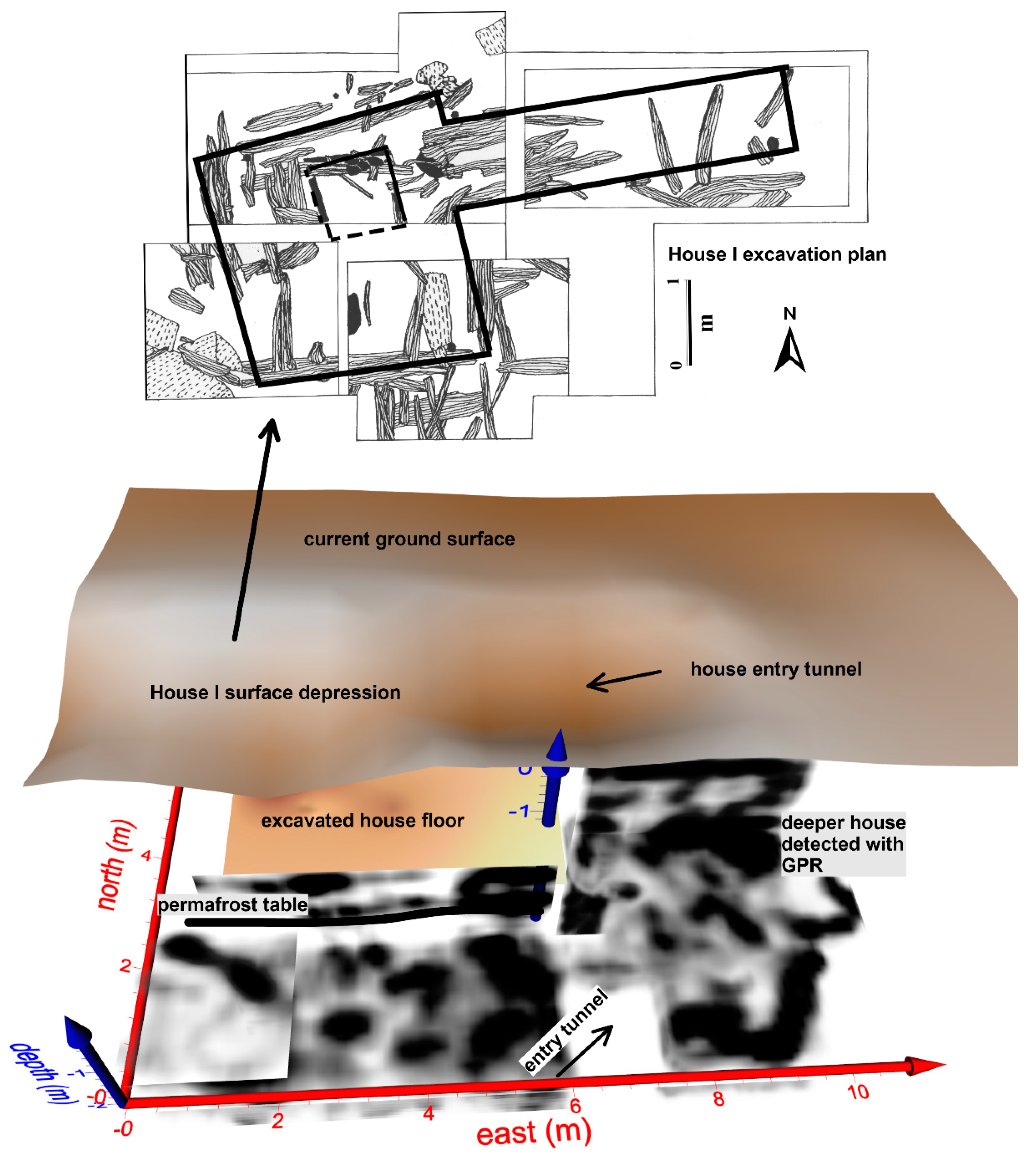
3.2.1. A Birnirk House Complex at Cape Espenberg, Bering Land Bridge National Preserve

Over the past seven years, a team of researchers has been excavating and studying the remains of a series of semi-subterranean house features that document the cultural transition from Birnirk to Thule of the Northern Maritime tradition at Cape Espenberg, Bering Land Bridge National Preserve [25,26]. Cape Espenberg consists of a series of beach ridge formations that have accumulated horizontally for 5000 years [27], preserving within them a 4500-year-old archaeological record of human adaptation to environmental change [27,28,29,30,31]. One characteristic that delineates the Birnirk from the later Thule culture is the apparent variety and complexity of house designs, some of which include many connected rooms, while others are reminiscent of the later Thule forms [31,32,33]. Typical Thule houses tend to have one main room with a long entrance tunnel and often a kitchen alcove off to one side [32] (p. 81). A recent study by Darwent et al. [27] used attributes of surface depressions to assess whether house shape and design at Cape Espenberg showed evidence for change through time. The results indicate designs evolved from complex multi-room structures towards simple one-room houses with straight tunnels. Excavations by Hoffecker and Mason’s 2011 team [25] found that among six house depressions excavated on three beach ridges, house floors could be located beneath apparent depressions in all cases but one. In the latter, no clear house feature was found except for a deeply build tunnel which suggests potential reuse of structural wood to build new houses. This raised the question: can GPR be used to locate deeply buried house features with sufficient resolution to demarcate the design and dimensions?
To answer this question we initiated a study at Cape Espenberg using GPR to collect data from a series of depressions thought to contain buried house ruins. The goal was to non-invasively document house design, floor configuration, and tunnel directions. Processing and interpreting the data was complicated by the fact that portions of the same feature-complex straddled the boundary of the active and frozen layers (Figure 7), thus involving two different GPR velocities as shown in Table 1. To deal with this situation, separate velocity estimates were undertaken for these two layers and data processing adjusted accordingly (Figure 8). The results show that not only are structural elements detectable but cultural deposits extend as deep as 3 m and indicate multiple structures, possibly floors, with cache pits present at many levels. This likely indicates multiple rebuilding events (Figure 9 and Figure 10). The GPR results also show that many of these features are located below the active layer, exceeding 1 m deep (Figure 7) but still resolvable with GPR (Figure 9 and Figure 10). While such frozen material bodes well for preservation of organic artifacts, it is a limiting factor for timely excavation where field seasons are short. These results suggest that the design history of the buried houses, particularly on the Birnirk beach ridge, appears much more complex than indicated from the surface. Interestingly, however, results show the appearance of a room that connects to one that was excavated at about the same depth (Figure 10 and Figure 11). The layout of these house structures resemble, perhaps not superficially, the sketch maps of house features recorded at the Birnirk site near Barrow [33] (p. 38) and Jabbertown at Point Hope [34] (p. 171). This provides further support for the hypothesis that Birnirk people were present at Cape Espenberg and that some of their settlements included multi-roomed house designs. Planned excavations will provide an opportunity to not only confirm these hypotheses but to refine the analytical method as well.

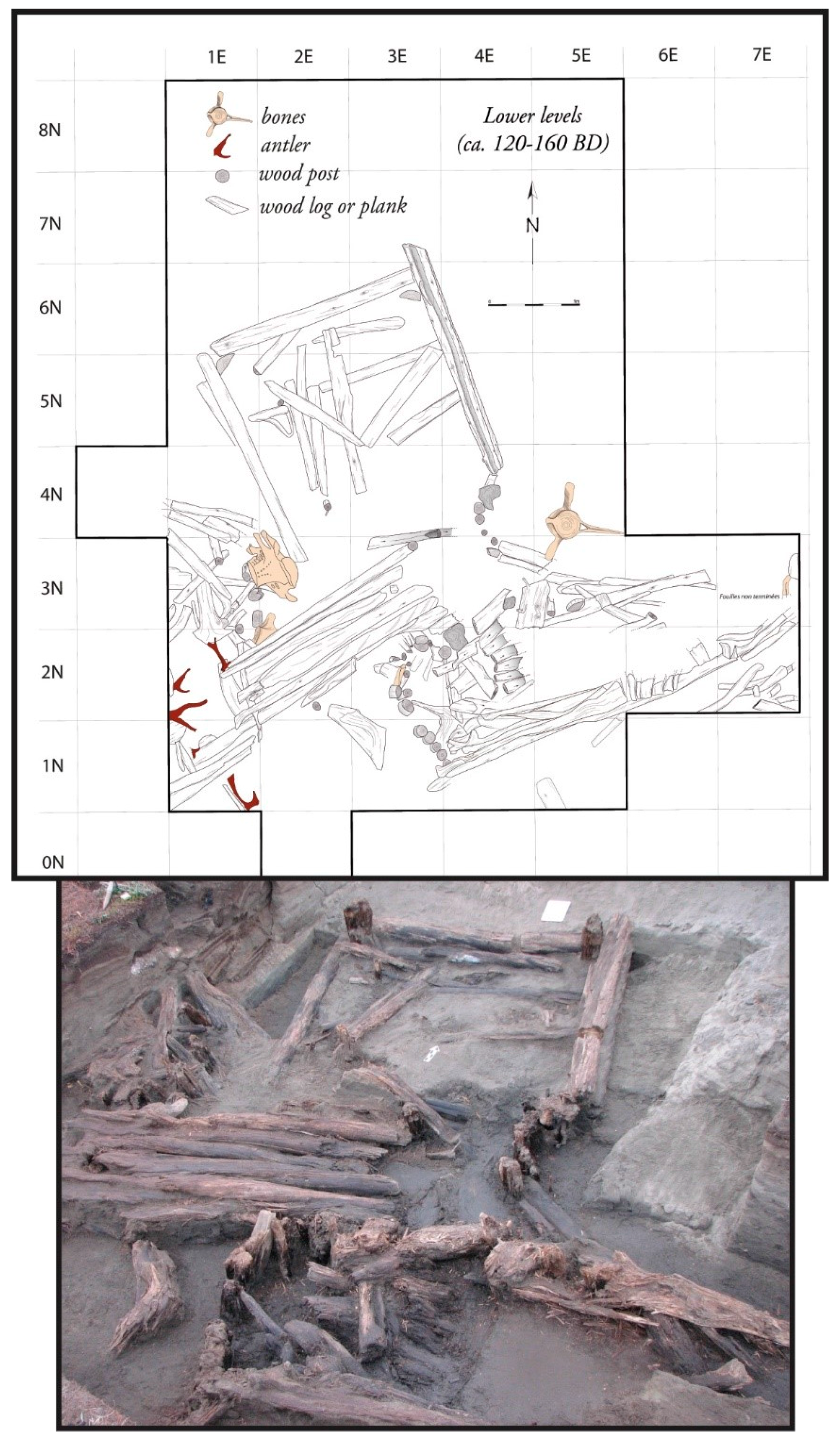
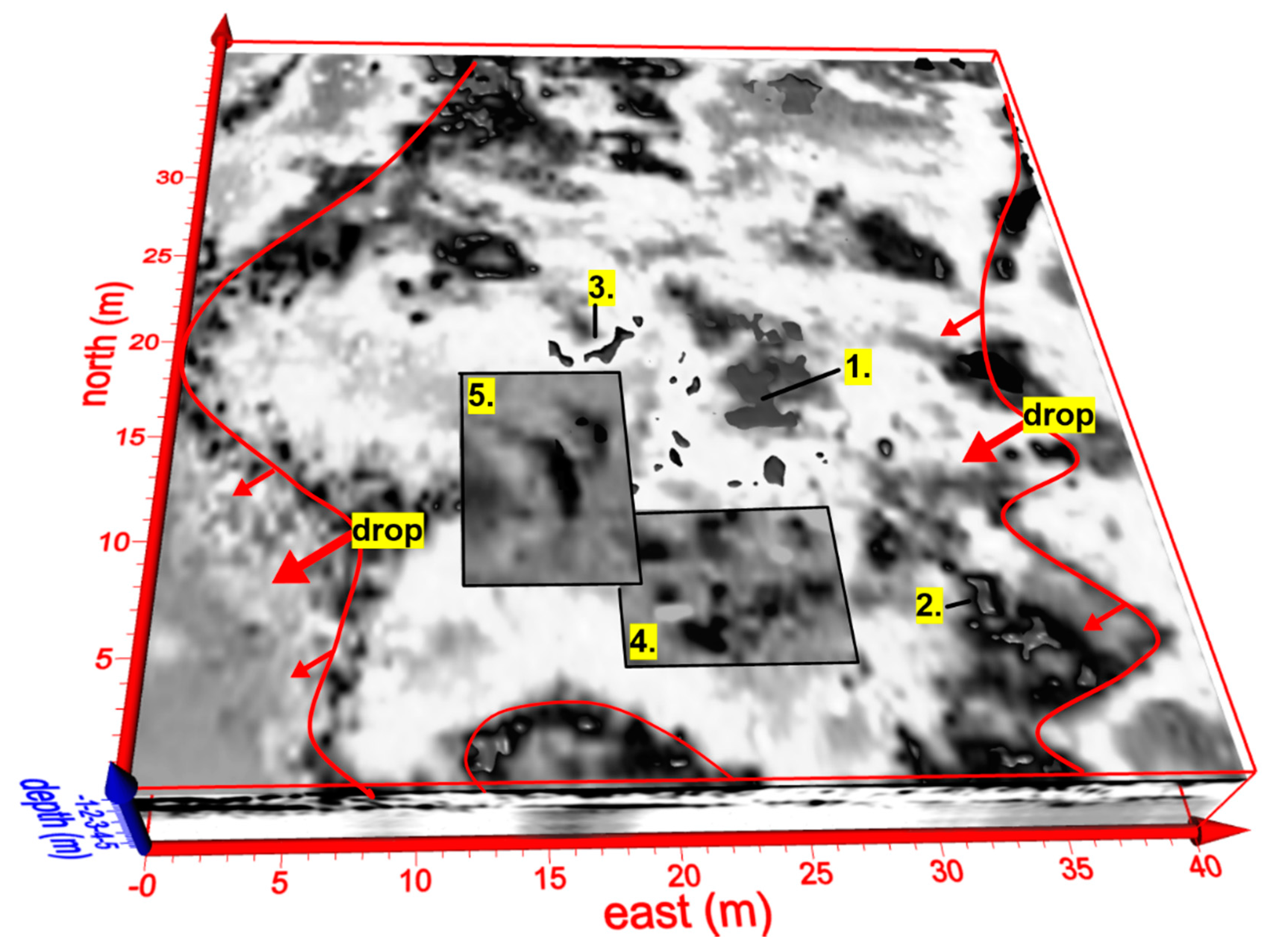
3.2.2. A Village Site at Kobuk Valley National Park with an Earlier Site below the Permafrost Table

The Kobuk River valley (see Figure 1) has been the site of numerous woodland Eskimo settlements spanning thousands of years [34,35,36,37,38,39]. Compared to Bering Land Bridge and Cape Krusenstern, the village site of Igliqtiqsiugvigruaq in Kobuk Valley National Park has the added challenge of being a forested site, where trees and vegetation limit the application of GPR [2]. The site is an early contact (19th-century) Inupiat village with evidence of limited Euro-American contact dating to around the time of the early 19th-century Euro-American expeditions in the region e.g., [40,41]. Geophysical investigations at the site involved three methods: GPR, magnetic gradiometry, and electromagnetic induction (EM). Insights derived from this work included not only understandings of the visible house pits and other village features [2], but also the discovery of a deeper, earlier settlement beneath the thawed active layer. The initial GPR work completed at the site in 2011 focused on areas in between the visible house depressions as these were assumed to be devoid of structures. The sole exception was a small strip south of House I, the ongoing excavation of which had suggested a possible tunnel extending from the house perimeter. Broader surveys undertaken in 2013, in search of additional tunnels, revealed (in addition to shallower features likely contemporary to the known village) evidence of a deeper occupation throughout the site, within the frozen layer beneath the known village (Figure 12 and Figure 13). Since the substrate in this case exhibited less water content at the time of data collection than the previous cases shown for Bering Land Bridge or Cape Krusenstern, a much smaller disparity between the velocities (i.e., dielectric properties) of active and frozen layers was evident. The permafrost depth encountered during the excavation of House I was consistent with GPR depth estimates from the surrounding area.
In addition to the deeper house detected with GPR in the vicinity of House I, many other deeper structures were detected throughout this sprawling village site, suggesting that the area had been a site of significant occupations prior to the 19th-century village. Though these deeper features remain untested archaeologically, optically stimulated luminescence (OSL) dating of sediments just beneath the floor of House I suggests that the deeper structures are likely at least several centuries older than the village.

3.3. Fully Frozen Settings: Bering Land Bridge and Gates of the Arctic

In the final two case studies, we present GPR results from fully frozen media. These results are more experimental and speculative than results from the known human occupations already presented. These, we believe, demonstrate the incredible potential for using GPR in frozen archaeological contexts other than known sites of human occupation, while recognizing that these two case studies provide less definitive results than the houses mapped with GPR at Bering Land Bridge and Kobuk Valley.

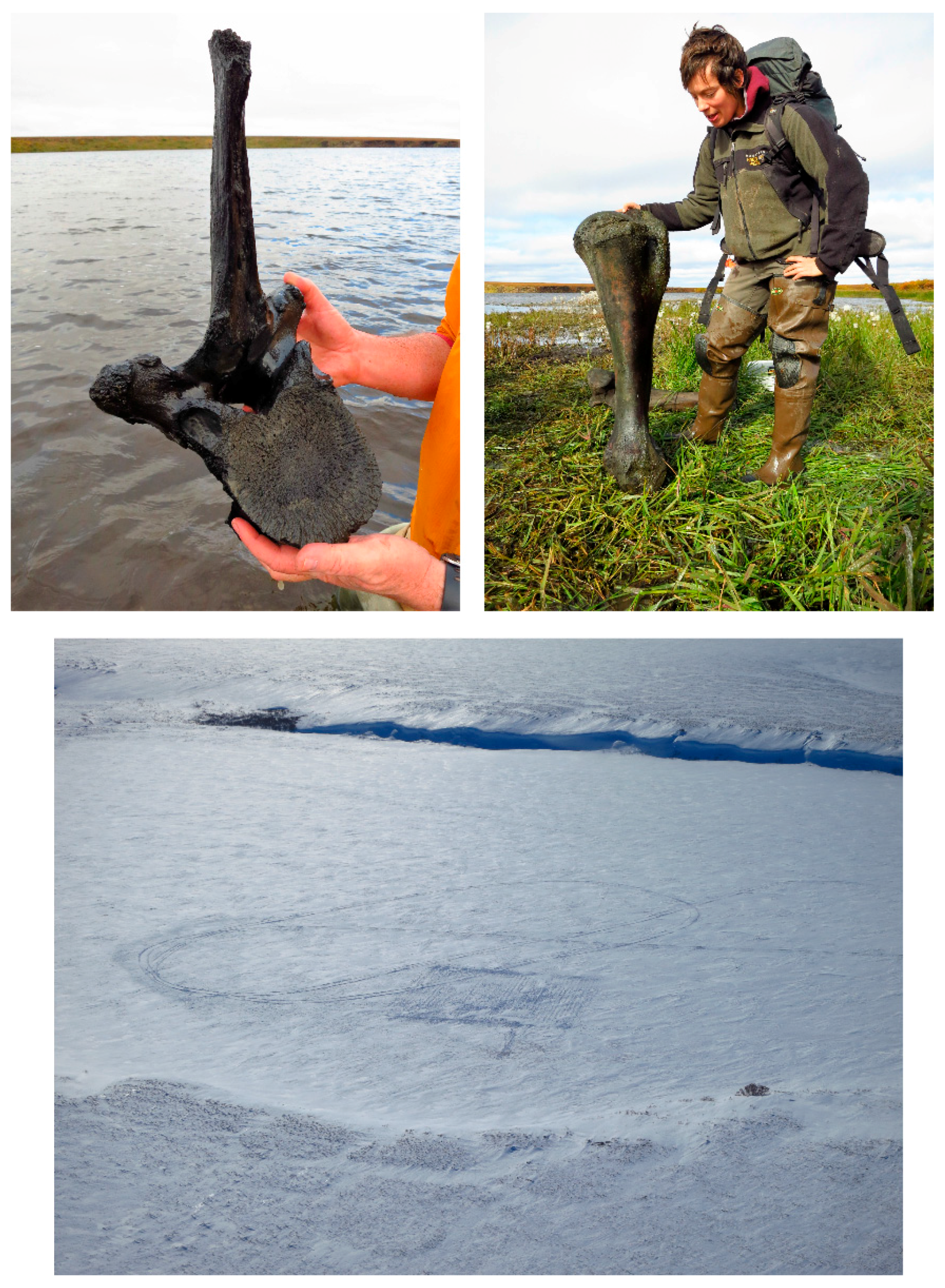
3.3.1. The Bering Land Bridge Mammoth

In 2015, a GPR survey was conducted on a frozen thermokarst lake in Bering Land Bridge National Preserve (see Figure 1) in order to assess the distribution of skeletal remains of a woolly mammoth (Mammuthus primigenius), and more generally to test the feasibility of using GPR to detect paleontological remains in such contexts (Figure 14). Several skeletal components from a single mammoth were located in 2012 on, and embedded within, the muddy bed of a shallow thermokarst lake. The skeletal materials were shallowly submerged and only identified due to a period of unusually low lake levels. They remained, however, very difficult to access and inventory due to their submerged and partially buried context. The site appears to have multiple elements from a single individual and may contain a complete or largely complete skeleton, which is rare for the region. Collagen from two mammoth bones collected from the site (KTZ-00345), a tooth and a vertebra, were radiocarbon dated to 12,330 ± 50 BP (Beta-329841, 12,720–12,140 Cal BC) and 12,430 ± 50 BP (Beta-331336, 12,940–12,220 Cal BC), respectively. A total of seven faunal components were identified in 2012 with osteological examination indicating that these were likely from an individual mammoth rather than a co-mingled deposit. GPR was used in an experimental attempt to detect and more fully map the distribution of additional skeletal material in this poor visibility setting, and further assess the completeness of the skeleton and the degree to which faunal components had been dispersed. GPS coordinates recorded for several skeletal components identified in 2012 were used for the later GPR investigation and allowed us to establish a geo-referenced grid around the coordinates of the previously investigated mammoth bones. The GPR data were collected from the frozen surface of the lake, which provided an excellent flat and unobstructed platform for the GPR survey.
Multiple anomalies consistent with a scatter of mammoth skeletal remains are evident on the lake floor (Figure 15). Several of these anomalies can be co-located with GPS-recorded locations of specific bones identified during the 2012 site reconnaissance. Immediately west of these marked locations are several anomaly clusters, which suggest additional skeletal material, including linear, curved anomalies that match the size and shape of tusks—skeletal elements expected to occur but not identified during the 2012 field investigations. Other discrete or clustered anomalies seen between the survey surface and lake bottom may represent additional skeletal remains, clusters of aqueous vegetation, or trapped gasses, all of which could result in abrupt changes in electrical properties thus generating GPR anomalies. Some of these anomalies seem to occur in association with broader morphological trends that could in turn act to trap accumulated debris. It is unlikely given the location of the lake that any of the GPR anomalies could be related to logs or rocks since these are not present in the area. All of the anomalies noted in Figure 15 are at the identified depth of the lake bottom, on a fairly flat, shallow shelf. Features detected with GPR beneath this interface appear to be natural cryogenic features (Figure 16). The GPR manifestation of these deeper features is comparable to ice-wedge polygon features described by Munroe et al. [24].

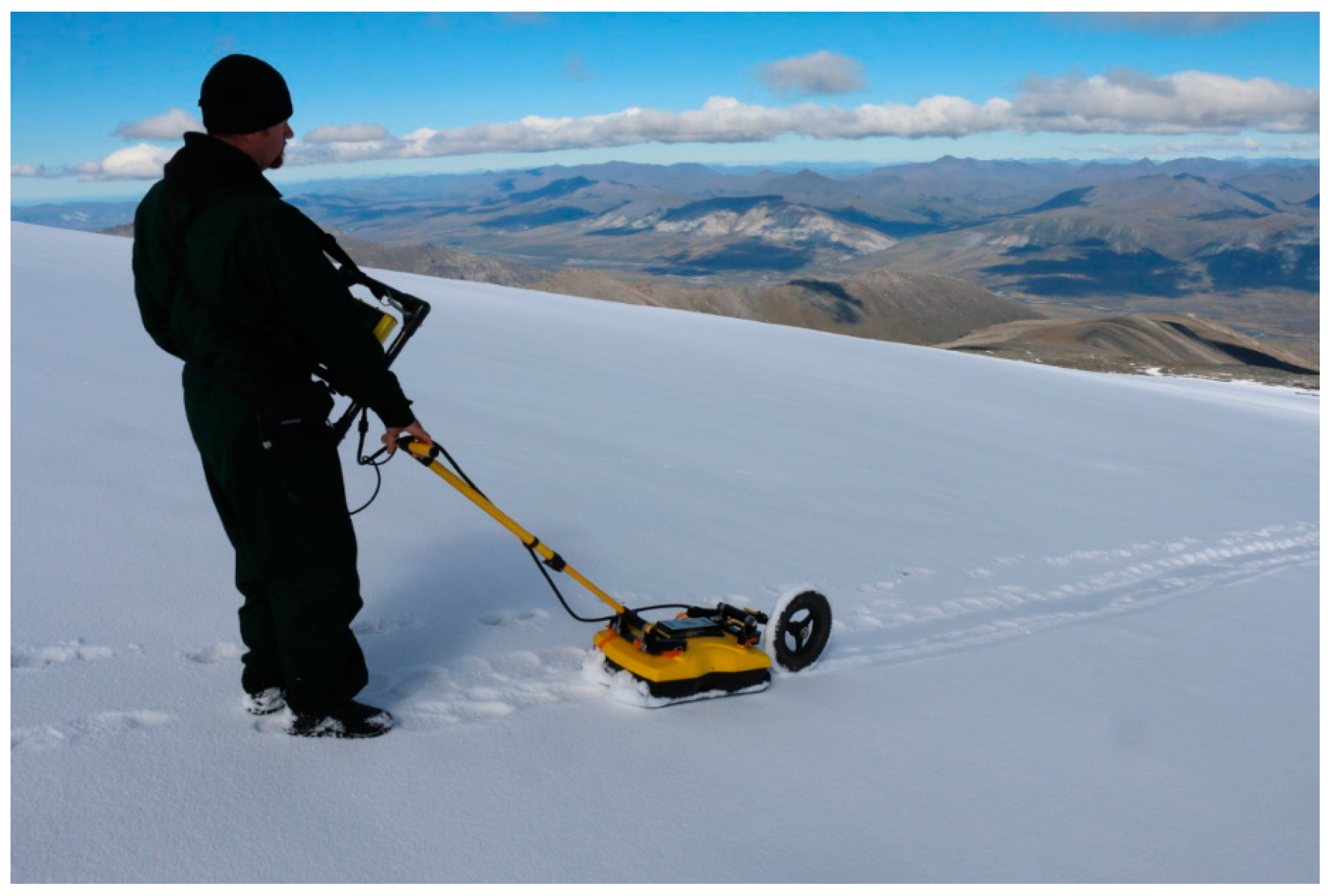
3.3.2. An Alpine Ice Field in Gates of the Arctic National Park and Preserve

Globally significant archaeological and paleoecological discoveries have been made in the last two decades in the surprising context of alpine snow patches and ice fields, which can contain well-preserved perishable objects of the sort rarely preserved in most archaeological contexts. Discoveries include an abundance of weaponry—arrow, spear and darts complete with intact wooden shafts, feather fletching and fiber lashings—as well as skin clothing and bark containers. Hunters understood that animals such as caribou congregated on snow-patches during certain seasons for insect relief and temperature regulation and they targeted game at these locations, occasionally losing tools and equipment in these natural freezers [42] (p. 313), [43]. High latitude and mountainous settings are prerequisite for these rare contexts, but not all regions seem to exhibit them in equal abundance. Particularly rich areas include British Columbia [44], southern Yukon Territory [43] and Northwest Territories [45,46] in Canada, areas of interior Alaska [47,48] and the Rocky Mountains in the western United States [49], and portions of Scandinavia and the European Alps [50]. The significance of ice patch finds stems from their ability to provide unique insights into prehistoric cultural developments and technology since these perishable items are rare in the vast majority of archaeological contexts. These same deposits often also contain rich assemblages of well-preserved plant and animal remains that can shed light on long-term environmental change [51]. There is an urgency to learn about these unique frozen archives because, across broad areas of the globe, glaciers and alpine ice patches are melting at a rate not seen for hundreds or thousands of years [52].
Despite substantial research efforts in many areas now spanning almost two decades, this resource is still not well-inventoried or well-understood in most areas. Great effort is required to find these small features in what is almost always rugged and remote terrain, and that must occur within narrow seasonal windows of maximum melting. The central Brooks Range within Gates of the Arctic National Park and Preserve (GAAR) is one area with good potential for snow patch finds, but within which very few have been documented. Reconnaissance surveys, ethnographic accounts, and reports from local residents have highlighted several dozen snow patch locations with potential to contain archaeological and paleoecological materials and examination of these locations is ongoing.
In 2016 our field team examined a low sloping ice field in GAAR (see Figure 1), at an elevation of ca. 2150 m above mean sea level (AMSL), to test the feasibility of using GPR in ice and snow patch investigation. This particular area was selected as one that would be accessible by both caribou and people, and therefore have reasonable archaeological potential. This alpine ice-field was accessed by helicopter, and nearly 1 km of GPR profiles were collected (Figure 17). All profiles clearly showed the type of reflections from internal bedding and diffractions from embedded targets that would be crucial for archaeological and paleo-environmental investigations of such features (Figure 18 and Figure 19). Our findings show that GPR, when paired with coring and surface investigations at the melt-zone of such features, could prove useful in identifying areas where archaeological deposits are likely to occur and may be subject to future loss due to melting. Though only in the trial stage, we believe that GPR could offer a major contribution to research and resource management for these threatened sites. The high-resolution measurement of the ice patch depth and cross-section can provide a useful means to monitor changing conditions of ice patches and track melting, though it should be noted that ice thickness and volume estimation can be subject to error [53]. Although layers of caribou dung—typically a key indicator of the presence of cultural materials—were not present in this ice patch, GPR methods would be well suited to detecting dung layers and mapping or quantifying their frequency, depth, and areal extent, which could help to identify the most productive ice patches for regular monitoring. The example shown here demonstrates the feasibility of deploying GPR in such cases.

4. Conclusions

Ground-penetrating radar (GPR) has been shown to be useful for addressing archaeological (and closely related paleoecological, geological and paleontological) questions in a range of settings in Arctic Alaska, including both partially frozen and fully frozen contexts. A number of straightforward lessons can be taken from this work to guide future research and resource management efforts:
  • Seasonal changes in the depth and character of the active layer influence the results of GPR surveys. In areas with substantial soil moisture, it may make sense to survey when active layer thickness reaches its seasonal maximum. The ground may be waterlogged, however, and penetration can be ensured by using a moderate antenna frequency as used in the examples shown here. Shortened wavelengths due to the high water content may allow excellent spatial and temporal resolution even with lower antenna frequencies.
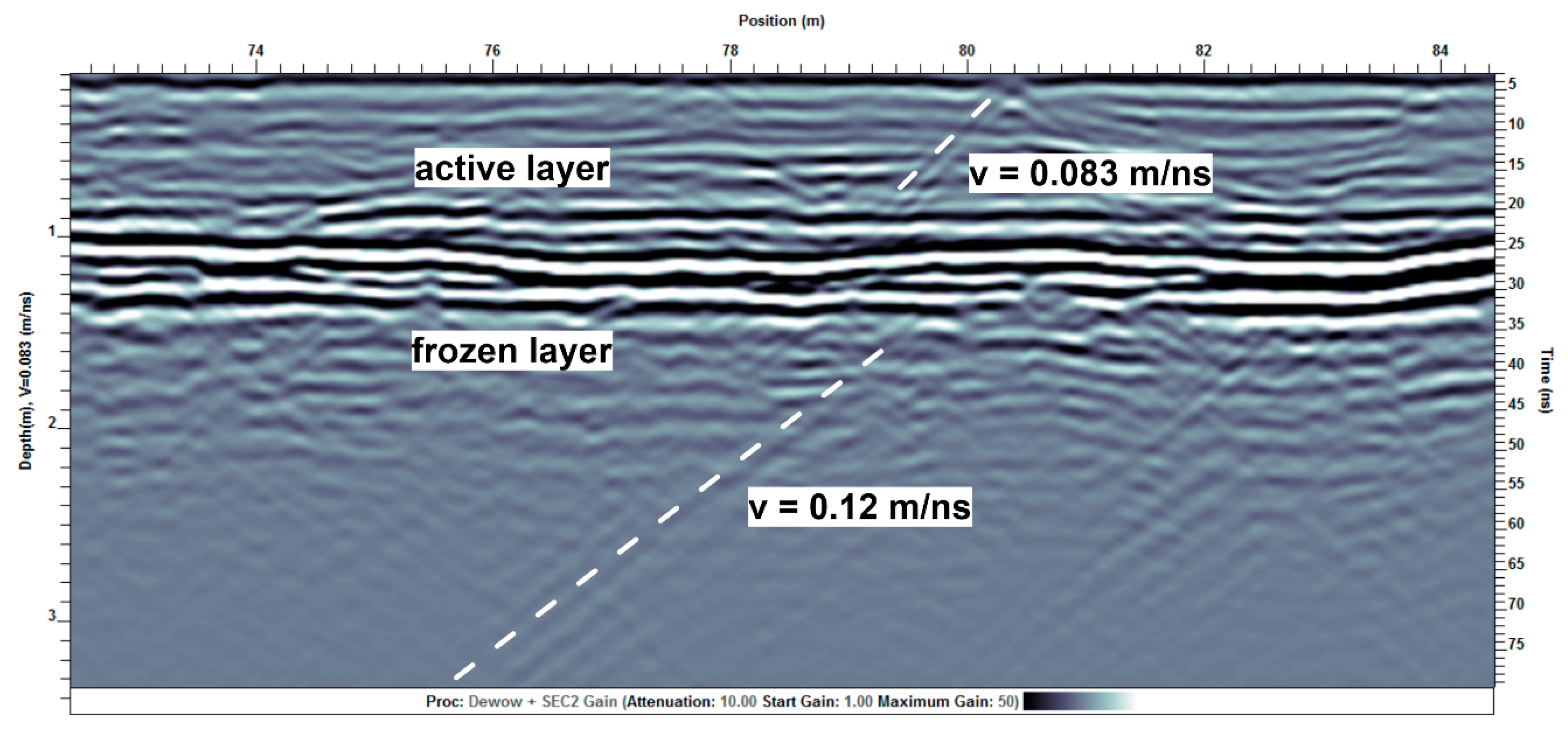
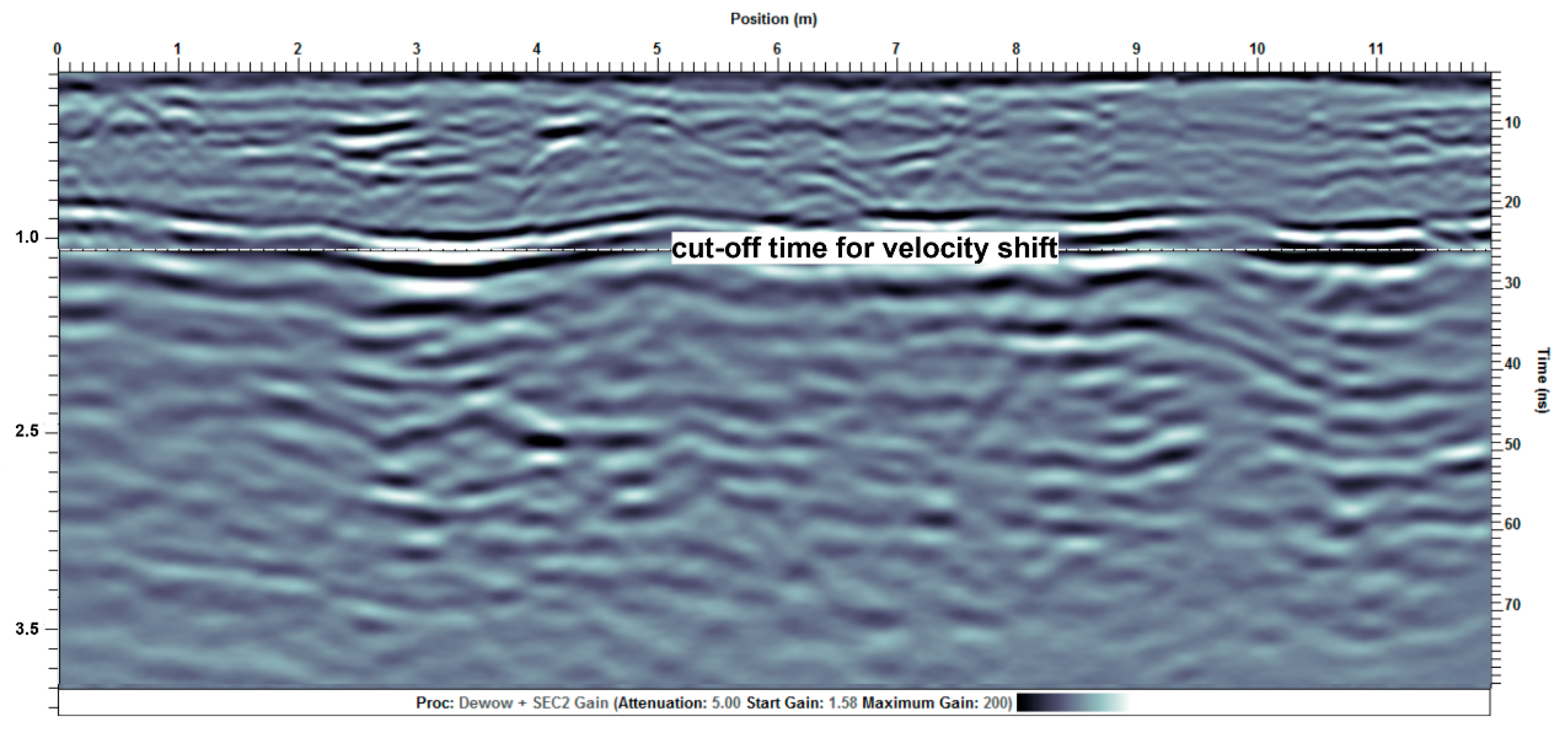
  • Accurate velocity determinations are critical for estimating both depth and dimensions of archaeological features and are therefore the most crucial parameters to be assessed. In partially frozen substrates, great care should be taken to consider the multiple velocities likely represented in the medium, which may in some cases exhibit extreme shifts, such as when a slow, wet layer is overlying a fast, frozen layer.
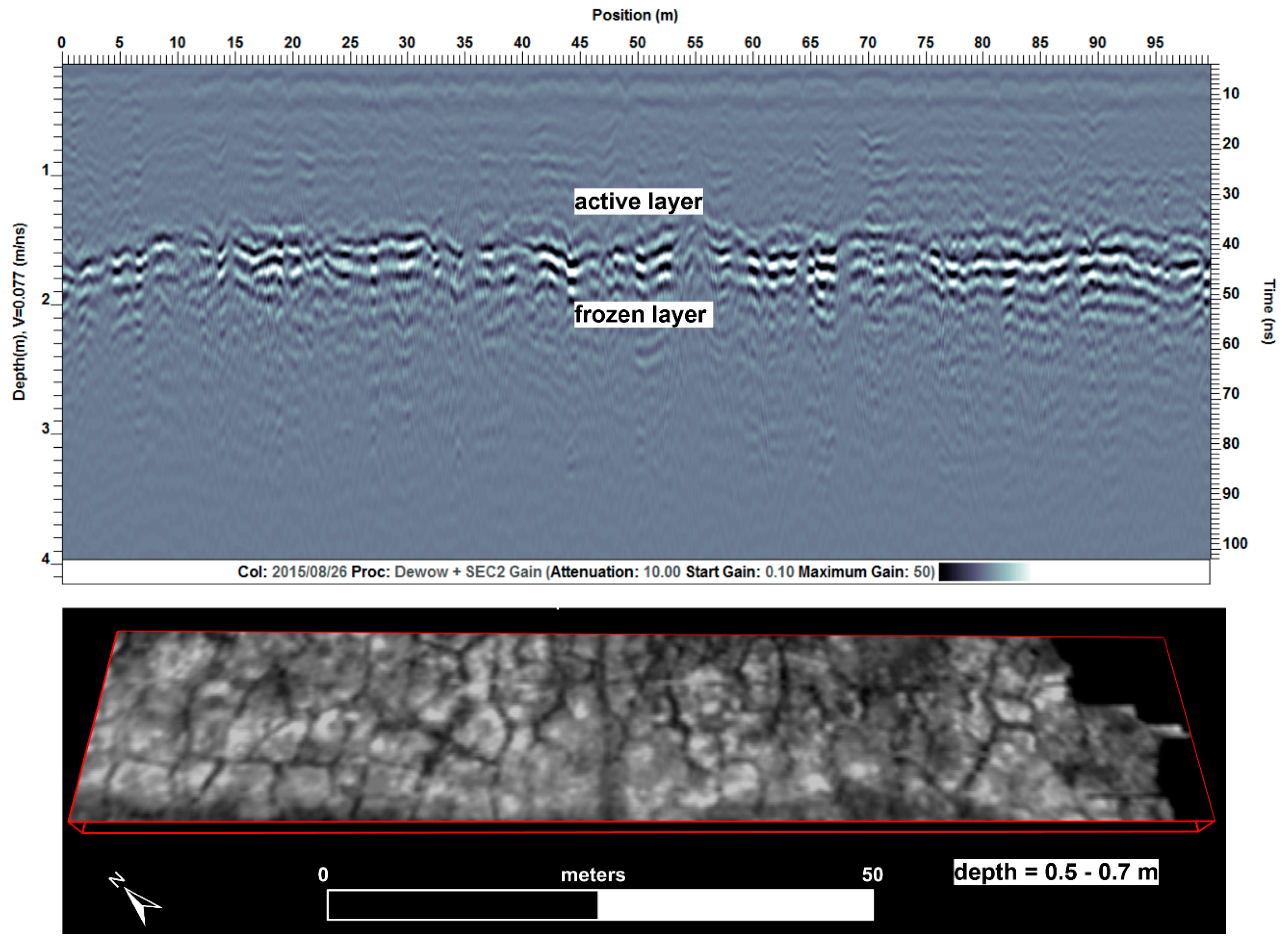
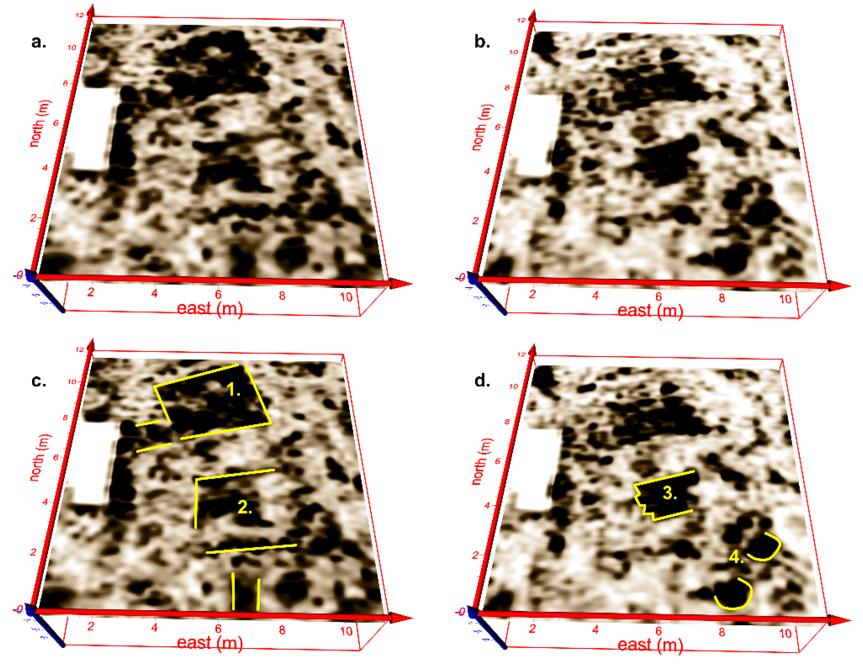
  • Patterns generated by freeze-thaw processes can be mistaken for cultural features such as house remains. Care should therefore be taken to understand how natural variations within a given survey setting are manifest in GPR data.
  • In fully frozen contexts, attenuation is limited and wavelengths are correspondingly increased with velocity. Surveying with higher antenna frequencies than those used for the examples in this paper may be warranted in order to maximize resolution. It must be kept in mind that not all surfaces encountered (e.g., snow) are amenable to the highest antenna frequencies due to difficulty of surface traverse and impracticability of the very closely spaced traverses that might be required to optimize horizontal resolution.
The central goal of cultural resource management is to learn about and protect significant heritage resources, a task that GPR and other geophysical methods aid tremendously in doing. These tools allow archaeologists and other specialists to effectively gather useful information about what lies below the ground, yielding data of direct value in portraying cultural features, documenting geologic contexts, and understanding site-formation processes. Geophysical data, including GPR, also plays an important role in designing smart sampling approaches that allow archaeologists to be judicious and focused with destructive means of data collection like excavation. Furthermore, geophysical techniques allow archaeologists to both target features of interest such as houses and hearths, and also to avoid impacting features such as burials, which no one wants to uncover without careful consideration, consultation, respect and appropriate means. This means that under the auspices of resource management, GPR may be included in aspects of tribal consultation. Though no examples were included in the study, our team has used GPR to locate tribal cemeteries in several regions of Alaska, often with indigenous stakeholders participating in the fieldwork. With the Kobuk Valley case study in the paper, local Inupiat community members participated in various aspects of the project, including the geophysical surveying.
We believe that the potential of GPR for frozen and partially frozen archaeological contexts has yet to be fully exploited and that this is a research and resource management area in need of further development, particularly with high latitude and high altitude archaeological resources facing threats from global environmental change. While GPR results are sometimes ambiguous, when used in tandem with other field methods such as excavation, auguring, and additional geophysical techniques, uncertainty can be reduced. In the coming years, GPR is likely to play an increasingly important role in the archaeology of frozen environments.

Acknowledgments

Work presented here from GAAR, BELA, and CAKR was funded by NPS National Center for Preservation Technology and Training (NCPTT) grant NPS-P15AP00094, as well as Cooperate Ecosystem Study Unit (CESU) agreements NPS-P14AC01303 and NPS-P16AC0052, awarded to Cornell University. Work in Kobuk Valley was funded by NSF awards 0908162 and 0908462 to Douglas A. and Wanni W. Anderson, and initial work at CAKR was funded by NSF award 1048194 to Christopher Wolff. Work at Cape Espenberg was funded by NSF awards ARC-0755725 to John F. Hoffecker and Owen K. Mason and award ARC-1523160 to Claire Alix and Owen K. Mason. We also thank Chris Ciancibelli and Tracy Asicksik for assistance with mapping and graphics.

Author Contributions

Thomas Urban collected and processed the GPR data presented in this paper and organized the initial draft, the overall concept of which is attributed to an NCPTT award developed by Manning, Rasic, and Urban. Fieldwork for the GAAR ice field survey and BELA (mammoth) survey was conducted by Urban and Rasic and the associated sections of the paper were authored initially by Rasic and Urban. Fieldwork for BELA (Cape Espenberg) was conducted by Urban and Tremayne under the direction of Alix and Mason. The BELA (Cape Espenberg) section was co-authored by Tremayne, Alix, Mason, and Urban. Fieldwork undertaken at CAKR included Urban, Wolff (2011), and Tremayne (2016), and the section on CAKR was authored by Wolff and Urban. Fieldwork at KOVA was conducted by Urban under the direction of Anderson, and the KOVA section was co-authored by Anderson and Urban. All co-authors made substantial edits to the overall text.

Conflicts of Interest

The authors declare no conflict of interest.

References

  1. Urban, T.M. In the footsteps of J. Louis Giddings: Archaeological geophysics in Arctic Alaska. Antiquity 2012, 85, 332. [Google Scholar]
  2. Urban, T.M.; Anderson, D.D.; Anderson, W.W. Multimethod geophysical investigations at an Inupiaq village in Kobuk Valley, Alaska. Lead. Edge 2012, 31, 950–956. [Google Scholar] [CrossRef]
  3. Wolff, C.; Urban, T.M. Geophysical analysis at the Old Whaling site, Cape Krusenstern, Alaska, reveals the possible impact of permafrost loss on archaeological interpretation. Polar Res. 2013, 32, 19888. [Google Scholar] [CrossRef]
  4. Urban, T.M.; Rasic, J.; Buvit, I.; Jacob, R.W.; Richie, J.; Hackenberger, S.; Hanson, S.; Ritz, W.; Wakeland, E.; Manning, S.W. Geophysical investigation of a middle Holocene site on the Yukon River, Alaska. Lead. Edge 2016, 35, 345–349. [Google Scholar] [CrossRef]
  5. Jacob, R.W.; Urban, T.M. Ground-penetrating radar velocity determination and precision estimates using common-mid-point (CMP) collection with hand-picking, semblance analysis, and cross-correlation analysis: A case study and tutorial for archaeologists. Archaeometry 2015. [Google Scholar] [CrossRef]
  6. Conyers, L.B. Ground-Penetrating Radar for Archaeology, 3rd ed.; AltaMira Press: Lanham, MD, USA, 2013. [Google Scholar]
  7. Annan, J.P. Ground Penetrating Radar: Principles, Procedures and Applications; Sensors and Software Inc.: Mississauga, ON, Canada, 2004. [Google Scholar]
  8. Cross, G.M.; Knoll, M.D. Diffraction-based velocity estimates from optimum offset seismic data. Geophysics 1991, 56, 2070–2079. [Google Scholar] [CrossRef]
  9. Al Hagrey, S.A.; Müller, C. GPR study of pore water content and salinity in sand. Geophys. Prospect. 2000, 48, 63–85. [Google Scholar] [CrossRef]
  10. Stolte, C. E-MIGRATION: Image Enhancement for Subsurface Objects of Constant Curvature in Ground Probing Radar Reflection Data. Ph.D. Thesis, Christian-Albrechts-Universität zu Kiel, Kiel, Germany, 1994. [Google Scholar]
  11. Arcone, S.A.; Delaney, A.J. Dielectric properties of thawed active layers overlying permafrost using radar at VHF. Radio Sci. 1982, 17, 618–626. [Google Scholar] [CrossRef]
  12. Davis, J.L.; Annan, J.P. Ground penetrating radar for high resolution mapping of soil and rock stratigraphy. Geophys. Prospect. 1982, 37, 531–551. [Google Scholar] [CrossRef]
  13. Daniels, D.J. Ground Penetrating Radar, 2nd ed.; The Institute of Electrical Engineers: London, UK, 2004. [Google Scholar]
  14. Goodman, D.; Piro, S. GPR Remote Sensing in Archaeology; Springer: Berlin/Heidelberg, Germany, 2013. [Google Scholar]
  15. Giddings, J.L. Ancient Men of the Arctic; Knopf, A.A., Ed.; University of Washington Press: Seattle, WA, USA, 1967. [Google Scholar]
  16. Giddings, J.L.; Anderson, D.D. Beach Ridge Archeology of Cape Krusenstern: Eskimo and Pre-Eskimo Settlements around Kotzebue Sound, Alaska; National Park Service: Washington, DC, USA, 1986.
  17. Ackerman, R.E. Settlements and sea mammal hunting in the Bering_Chukchi Sea region. Arct. Anthropol. 1988, 25, 52–79. [Google Scholar]
  18. Dikov, N.N. The oldest sea mammal hunters of Wrangel Island. Arct. Anthropol. 1988, 25, 80–93. [Google Scholar]
  19. Darwent, J.; Darwent, C.M. The occupational history of the Old Whaling site at Cape Krusenstern. Alask. J. Anthropol. 2005, 3, 135–153. [Google Scholar]
  20. Mason, O.K.; Gerlach, S.C. The Archaeological Imagination, Zooarchaeological Data, the Origins of Whaling in the Western Arctic, and ‘‘Old Whaling’’ and Choris Cultures. In Hunting the Largest Animals: Native Whaling in the Western Arctic and Subarctic; Studies in Whaling 3, 1_32; McCartney, A.P., Ed.; Canadian Circumpolar Institute: Edmonton, AB, Canada, 1995. [Google Scholar]
  21. Darwent, C.M. Reassessing the old whaling locality at Cape Krusenstern, Alaska. In Proceedings of the SILA/NABO Conference on Arctic and North Atlantic Archaeology, Copenhagen, Denmark, 10–14 May 2004.
  22. Selby, M.J. Earth’s Changing Surface: An Introduction to Geomorphology; Oxford University Press: Oxford, UK, 1996. [Google Scholar]
  23. Hinkel, K.M.; Doolittle, J.A.; Bockheim, J.G.; Nelson, F.E.; Paetzold, R.; Kimble, J.M.; Travis, R. Detection of subsurface permafrost features with ground-penetrating radar, Barrow, Alaska. Permaf. Periglac. Process. 2001, 12, 179–190. [Google Scholar] [CrossRef]
  24. Munroe, J.S.; Doolittle, J.A.; Kanevskiy, M.Z.; Hinkel, K.M.; Nelson, F.E.; Jones, B.M.; Shur, Y.; Kimble, J.M. Application of ground-penetrating radar imagery for three-dimensional visualisation of near-surface structures in Ice-Rich Permafrost, Barrow, Alaska. Permafr. Periglac. Process. 2007. [Google Scholar] [CrossRef]
  25. Hoffecker John, F.; Mason, O.K. Human Response to Climate Change at Cape Espenberg: AD 800–1400; University of Colorado: Boulder, CO, USA, 2011. [Google Scholar]
  26. Alix, C.; Mason, O.K.; Mason Bigelow, N.H.; Anderson, S.L.; Rasic, J.; Hoffecker, J.F. Archéologie du cap Espenberg ou la question du Birnirk et de l’origine du Thule dans le nord-ouest de l’Alaska. Nouv. l’Archéol. 2015, 141, 13–18. [Google Scholar] [CrossRef]
  27. Darwent, J.; Mason, O.K.; Hoffecker, J.F.; Darwent, C.M. 1000 years of house change at Cape Espenberg, Alaska: A case study in horizontal stratigraphy. Am. Antiq. 2013, 78, 433–455. [Google Scholar] [CrossRef]
  28. Mason, O.K. Sand ridge stratigraphy of the northern seward peninsula. In Bering Land Bridge National Preserve: An Archeological Survey; National Park Service Resource/Research Management Report AR-14; Schaaf, J., Ed.; U.S. Department of the Interior: Washington, DC, USA, 1988; Volume 1–2, pp. 364–409. [Google Scholar]
  29. Harritt Roger, K. Eskimo Prehistory on the Seward Peninsula, Alaska; National Park Service Resource/Research Management Report ARORCR/CRR-93/21; U.S. Department of the Interior, Alaska Regional Office: Anchorage, AK, USA, 1994.
  30. Mason, O.K.; Hopkins, D.M.; Plug, L. Chronology and paleoclimate of storm-induced erosion and episodic dune growth across Cape Espenberg Spit, Alaska, USA. J. Coast. Res. 1997, 13, 770–797. [Google Scholar]
  31. Schaaf, J. Bering Land Bridge National Preserve: An Archeological Survey; National Park Service Resource/Research Management Report AR-14; U.S. Department of the Interior: Washington, DC, USA, 1988; Volume 1–2.
  32. Tremayne, A.H. New evidence for the timing of arctic small tool tradition coastal settlement in Northwest Alaska. Alask. J. Anthropol. 2015, 13, 1–18. [Google Scholar]
  33. Anderson Douglas, D. Prehistory of North Alaska. In Handbook of North American Indians, Volume 5: Arctic; Damas, D., Ed.; Smithsonian Institution Press: Washington, DC, USA, 1984; pp. 80–93. [Google Scholar]
  34. Ford, J.A. Eskimo prehistory in the vicinity of point Barrow, Alaska. Am. Mus. Nat. Hist. 1959, 47, 1. [Google Scholar]
  35. Larsen, H.; Rainey, F. Ipiutak and the Arctic Whale Hunting Culture; American Museum of Natural History: New York, NY, USA, 1948. [Google Scholar]
  36. Giddings, J.L. Arctic Woodland Culture of the Kobuk River; Museum Monographs, The University Museum, University of Pennsylvania: Philadelphia, PA, USA, 1952. [Google Scholar]
  37. Giddings, J.L. Forest Eskimos; University Museum Bulletin: Philadelphia, PA, USA, 1956. [Google Scholar]
  38. Giddings, J.L. Kobuk River People; No. 1. College: University of Alaska: Fairbanks, AK, USA, 1961. [Google Scholar]
  39. Anderson, D.D. Onion Portage: The archaeology of a stratified site from the Kobuk River, Northwest Alaska. Anthropol. Pap. Univ. Alask. 1988, 22, 1–163. [Google Scholar]
  40. Von Kotzebue, O. A Voyage of Discovery, into the South Sea and Beering’s Straits, for the Purpose of Exploring a North-East Passage, Undertaken in the Years 1815–1818, at the Expense of His Highness Count Romanzoff, in the Ship Rurick, under the Command of the Lieutenant in the Russian Imperial Navy, Otto von Kotzebue; Longman: London, UK, 1821. [Google Scholar]
  41. Beechey, F.W. Narrative of a Voyage to the Pacific and Beering’s Strait, to Co-Opereate with the Polar Expeditions: Performed in His Majesty’s Ship Blossom, under the Command of Captain F.W. Beechey in the Years 1825, 26, 27, 28; Colburn, H., Bentler, R., Eds.; Cambridge University Press: Cambridge, UK, 1831; Volume 2. [Google Scholar]
  42. Binford, L.R. Nunamiut Ethnoarchaeology; Academic Press: New York, NY, USA, 1978. [Google Scholar]
  43. Hare, P.G.; Greer, S.; Gotthardt, R.; Farnell, R.; Bowyer, V.; Schweger, C.; Strand, D. Ethnographic and archaeological investigations of alpine ice patches in Southwest Yukon, Canada. Arctic 2004, 57, 260–272. [Google Scholar] [CrossRef]
  44. Beattie, O.; Apland, B.; Blake, E.W.; Cosgrove, J.A.; Gaunt, S.; Greer, S.; Mackie, A.P.; Mackie, K.E.; Straathoff, D.; Thorp, V.; et al. The Kwäday Dän Tsínchi Discovery from a Glacier in British Columbia, Candadian. J. Archaeol. 2000, 24, 129–147. [Google Scholar]
  45. Andrews, T.D.; MacKay, G.; Andrew, L. Archaeological investigations of alpine ice patches in the Selwyn Mountains, Northwest Territories, Canada. Arctic 2012, 65, 1–21. [Google Scholar] [CrossRef]
  46. Meulendyk, T.; Moorman, B.J.; Andrews, T.D.; MacKay, G. Morphology and development of ice patches in Northwest Territories, Canada. Arctic 2012, 65, 43–58. [Google Scholar] [CrossRef]
  47. Dixon, E.J.; Manley, W.F.; Lee, C.M. The Emerging archaeology of glaciers and ice patches: Examples from Alaska’s Wrangell-St. Elias National Park and Preserve. Am. Antiq. 2005, 70, 129–143. [Google Scholar] [CrossRef]
  48. Vander Hoek, R.; Wygal, B.; Tedor, R.M.; Holmes, C. Survey and monitoring of ice patches in the Denali highway region, Central Alaska, 2003–2005. Alask. J. Anthropol. 2007, 5, 67–86. [Google Scholar]
  49. Lee, C.M. Withering snow and ice in the mid-latitudes: A new archaeological and paleobiological record for the Rocky Mountain region. Arctic 2012, 65, 165–177. [Google Scholar] [CrossRef]
  50. Grosjean, M.; Suter, P.J.; Trachsel, M.; Wanner, H. Ice-borne prehistoric finds in the Swiss Alps reflect Holocene glacier fluctuations. J. Quat. Sci. 2007, 22, 203–207. [Google Scholar] [CrossRef]
  51. Farnell, R.; Hare, P.G.; Blake, E.; Bowyer, V.; Schweger, C.; Greer, S.; Gotthardt, R. Multidisciplinary investigations of alpine ice patches in Southwest Yukon, Canada: Paleoenvironmental and paleobiological investigations. Arctic 2004, 57, 247–259. [Google Scholar] [CrossRef]
  52. Bjork, R.G.; Molau, U. Ecology of alpine snowbeds and the impact of global change. Arct. Antarct. Alp. Res. 2007, 39, 1. [Google Scholar] [CrossRef]
  53. Martín-Español, A.; Lapazaran, J.J.; Otero, J.; Navarro, F.J. On the errors involved in ice-thickness estimates III: Error in volume. J. Glaciol. 2016. [Google Scholar] [CrossRef]
Figure 1. Study location. The boundaries of the National Parks and Preserves are indicated, including from East to West, Gates of the Arctic (GAAR), Kobuk Valley (KOVA), and Cape Krusenstern (CAKR), all in the Arctic Circle, and Bering Land Bridge (BELA) which straddles the boundary of the Arctic Circle.
Remotesensing 08 01007 g001
Figure 2. Diagrammatic model and equivalent electrical circuit for GPR pulse in a partially frozen setting.
Remotesensing 08 01007 g002
Figure 3. Fieldwork landing site at Bering Land Bridge. Shown: T. Urban. Photo by J. Rasic.
Remotesensing 08 01007 g003
Figure 4. Permafrost table in July 2016 at the Old Whaling Ridge. The frozen interface results in a sudden velocity increase, along with changes in diffraction tails that indicate an average velocity change. Here the active layer is ca. 1 m thick before frozen ground is encountered.
Remotesensing 08 01007 g004
Figure 5. The late summer (August) permafrost table at the Old Whaling Ridge. This is the full extent of the same monitoring station shown in Figure 5. A three-trace running average has been applied to emphasize horizontal reflectors. Note that the active layer extends nearly 1 m deeper than the mid-summer depth shown in Figure 5. The active layer exhibits a network of cracks from the freeze-thaw cycle, which are clear in plan-view GPR data (bottom). In isolation, perimeters of these frost polygons can easily be mistaken for cultural features in the sub-surface.
Remotesensing 08 01007 g005
Figure 6. Semi-subterranean house diagram.
Remotesensing 08 01007 g006
Figure 7. A sample GPR profile from Cape Espenberg. The permafrost interface is clear at 20–23 ns. The active layer exhibits an average velocity of 0.82 m/ns for a depth estimate to the frozen interface of ca. 1 m. This velocity, however, yields inaccurate depth estimates at depths greater than 1 m because the frozen ground exhibits an average velocity of 0.12 m/ns. This data set was collected within several days of the Cape Krusenstern 2016 expedition data and shows the frozen interface (and velocities) are comparable to those observed at the Old Whaling Ridge.
Remotesensing 08 01007 g007
Figure 8. Profile processed as a two-velocity medium. The average velocities of both the frozen and active layer from the same profile shown in Figure 7 were used to produce the above profile with accurate depth estimates for both layers. Depths in the frozen layer are tens of centimeters more than estimated with the active layer velocity alone. The profile above has also migrated using the velocity of the frozen layer. Note that the majority of diffraction tails have been reduced or eliminated when compared to the previous figure.
Remotesensing 08 01007 g008
Figure 9. (a) Portion of a Birnirk house complex in the active layer (upper meter) with layout and dimensions consistent with nearby excavated examples. The darker colors indicate higher amplitude reflections from buried wood, bone and other material as seen in the nearby excavation; (b) Portion of a Birnirk house complex in the frozen layer (extending below one meter) with layout and dimensions consistent with nearby excavated examples. This is a deeper portion of the same house complex shown in (a); (c) Annotated interpretations 1 and 2 indicated the proposed outline of structures interred from (a), along with likely tunnel locations. The orientation and scale of these features are comparable to the nearby excavation (Figure 10 and Figure 11), and the excavated and unexcavated structures are likely connected; (d) Annotations indicate a likely cluster of timbers, three, and external storage pits, four. Other discrete anomalies scattered throughout the survey area are likely caused by debris such as wood and whale bone external to the structures. This is also consistent with the nearby excavation.
Remotesensing 08 01007 g009
Figure 10. Feature 12 at Cape Espenberg KTZ304 site. Excavated area in 2011 to the west of the surveyed area shown in Figure 9. Depth excavated is 0.9 to 1.2 m below surface (map by Sylvie Elies and Claire Alix and photo by Claire Alix). Frozen material was encountered at depths consistent with the GPR estimates. The layout and complexity of deposits was also consistent with the GPR results shown in Figure 9 and Figure 10, which is immediately east of the Feature 12 excavation unit.
Remotesensing 08 01007 g010
Figure 11. The relationship of the excavated structure to the unexcavated features detected with GPR. The comparative scale and alignment of the known and inferred features is obvious. The GPR image (right) is a 3-D iso-surface showing high amplitude anomalies spanning a depth of ca. 0.5–1.2 m.
Remotesensing 08 01007 g011
Figure 12. GPR survey area around House I depression. The outline of a deeper house appeared in the GPR survey from a depth of 1.4–2.0 m, shown above as a series of depth-slices at 0.1 m increments. The projected perimeter of the deeper house is indicated in yellow in the final slice. GPR coverage was limited by the presence of trees at this forested site.
Remotesensing 08 01007 g012
Figure 13. House I. The surface depression designated House I was excavated to the house floor and dated to the 19th century. Permafrost encountered in the deepest portions of the excavation was consistent with an interface identified in the GPR survey around the depression. The GPR survey also showed an additional occupation in the frozen layer. Similar features were detected in other areas of the village site at comparable depths. The darker colors represent higher amplitude reflections. Our excavated cases at this site indicate that wood framing timbers are the cause of these anomalies.
Remotesensing 08 01007 g013
Figure 14. Top: Mammoth vertebra (left) and humerus (right) located in 2012. NPS photo, J. Rasic. (Shown: Louise Farquharson); Bottom: View of the mammoth bone scatter survey area from the air. Photo by J. Rasic 2015. The landing track of the plane as well as the grid pattern of the completed GPR survey are visible.
Remotesensing 08 01007 g014
Figure 15. Interpretation. (1) The location of four known skeletal components (ulna, humerus, rib, vertebra) clearly coincides with a cluster of GPR anomalies of various sizes; (2) The known location of two additional vertebrae also coincides with a cluster of GPR anomalies; (3) Several anomalies west of the main cluster on known skeletal components are suggestive in form of additional bones; (4) A cluster of anomalies on a plane just above the lake bottom exhibits several velocity/polarization oddities that may be related to frozen vegetation and/or trapped gas pockets along with additional bones; (5) Also shown on a plane just above the lake bottom, and perhaps most suggestive, is a pair of anomalies that exhibit forms consistent with tusks. All of these anomalies seem to be settled on (or embedded in) the lake bottom on a generally flat area located in between a shallow drop-off in the east (about a 25 cm drop) and a sloping drop in the west of somewhat greater magnitude.
Remotesensing 08 01007 g015
Figure 16. Just beneath the shallow lake bottom, the GPR data reveal patterns characteristic of ice wedge polygons. The interface of the silty lake bottom, upon which the mammoth bones rest is indicated in the profile (top). A deeper interface seen in the profiles may be due to a textural transition in the substrate, from finer-grain sediment to coarse gravel.
Remotesensing 08 01007 g016
Figure 17. T. Urban collecting GPR data on ice patch. Photo by J. Rasic 2016.
Remotesensing 08 01007 g017
Figure 18. An example of GPR data from an alpine ice patch shown in standard seismic color scheme. The bedrock is easily distinguished from the ice, while embedded anomalies generate clear diffraction hyperbolas (e.g., 1). These were used to determine a velocity of 0.17 m/ns. Bedding is clear throughout the ice (e.g., 2) indicating that the types of ancient surfaces that might contain archaeological material would be readily detectable with GPR. Such interfaces may also contain a range of paleo-environmental material relevant to archaeology.
Remotesensing 08 01007 g018
Figure 19. An example of GPR data from an alpine ice patch after attribute analysis (instantaneous amplitude envelope) and topographic corrections. This offers a more intuitive image with truer dimensions. This is the same profile as shown in Figure 18.
Remotesensing 08 01007 g019
Table 1. Common ground-penetrating radar (GPR) velocities for a range of materials in order of decreasing velocity. Compiled and adapted from [6,12,13,14].
MaterialVelocity (m/ns)
Air0.3
Snow0.2
Cold ice0.16–0.18
Temperate ice0.15
Permafrost0.12–0.14
Dry gravel0.12
Wet gravel0.10
Silt (wet)0.07
Clay (wet)0.06
Fresh water0.033
Table 2. Instrument and survey parameters.
Parameter
Gridded traverse(varied) anti-parallel, sometimes bi-directional
Transect interval(varied) 0.20–0.5 m
Trace interval0.05 m
Tx-Rx offset0.279 m
Time window(varied) 80–200 ns
Stacks8 per station

