Article

Multi-Range Conditional Random Field for Classifying Railway Electrification System Objects Using Mobile Laser Scanning Data

1
Department of Earth and Space Science and Engineering, York University, 4700 Keele Street, Toronto, ON M3J 1P3, Canada
2
Logistics System Research Team, Korea Railroad Research Institute, 176, Cheoldobangmulgwan-ro, Uiwang-si, Gyeonggi-do 16105, Korea
*
Author to whom correspondence should be addressed.
These authors contributed equally to this work.
Remote Sens. 2016, 8(12), 1008; https://doi.org/10.3390/rs8121008
Submission received: 27 September 2016 / Revised: 29 November 2016 / Accepted: 2 December 2016 / Published: 10 December 2016

Abstract

:
Railways have been used as one of the most crucial means of transportation in public mobility and economic development. For safe railway operation, the electrification system in the railway infrastructure, which supplies electric power to trains, is an essential facility for stable train operation. Due to its important role, the electrification system needs to be rigorously and regularly inspected and managed. This paper presents a supervised learning method to classify Mobile Laser Scanning (MLS) data into ten target classes representing overhead wires, movable brackets and poles, which are key objects in the electrification system. In general, the layout of the railway electrification system shows strong spatial regularity relations among object classes. The proposed classifier is developed based on Conditional Random Field (CRF), which characterizes not only labeling homogeneity at short range, but also the layout compatibility between different object classes at long range in the probabilistic graphical model. This multi-range CRF model consists of a unary term and three pairwise contextual terms. In order to gain computational efficiency, MLS point clouds are converted into a set of line segments to which the labeling process is applied. Support Vector Machine (SVM) is used as a local classifier considering only node features for producing the unary potentials of the CRF model. As the short-range pairwise contextual term, the Potts model is applied to enforce a local smoothness in the short-range graph; while long-range pairwise potentials are designed to enhance the spatial regularities of both horizontal and vertical layouts among railway objects. We formulate two long-range pairwise potentials as the log posterior probability obtained by the naive Bayes classifier. The directional layout compatibilities are characterized in probability look-up tables, which represent the co-occurrence rate of spatial relations in the horizontal and vertical directions. The likelihood function is formulated by multivariate Gaussian distributions. In the proposed multi-range CRF model, the weight parameters to balance four sub-terms are estimated by applying the Stochastic Gradient Descent (SGD). The results show that the proposed multi-range CRF can effectively classify individual railway elements, representing an average recall of 97.66% and an average precision of 97.07% for all classes.

Graphical Abstract

1. Introduction

From the beginning of human civilization, railway systems have played a critical role in economic development nationally and globally. In Canada alone, the railway systems cover 60,000 km of main track-line and transport 75 million people, as well as $250 billion worth of goods each year. Thus, it is evident that keeping the public transportation services efficient, safe and secure, increasing their mobility and having the railways contribute to economic growth are the top priorities for the rail transportation organization [1,2]. The electrification system is one of the key railway infrastructures in addition to the right-of-way, track, signaling and station [3]. The electrification system supplies the power that the train can access at all times. It must be safe, reliable, economical and user friendly. Therefore, rigorous inspection and frequent maintenance of the railway electrification system are essential and regular tasks. However, the railway infrastructure is still vulnerable to a number of potential risks, such as structural defects, equipment failure, vegetation encroachment, severe weather conditions, human factors, and so forth [2]. To mitigate such risks in a timely manner, today’s inspection practice mainly relies on labor-intensive visual inspection by humans traversing along the rail tracks. However, this traditional monitoring of rail electrification systems is tedious, time consuming and inaccurate [4].
Recently, various techniques using remotely-sensed data, such as images, Airborne Laser Scanning (ALS) data and Mobile Laser Scanning (MLS) data, have been introduced to supplement or replace humans’ visual inspection. In particular, MLS data provide very accurate and highly dense point clouds over the railway scene scanned by laser scanners mounted on a train or inspection cart. In previous studies, MLS data have been used to automatically recognize, detect and reconstruct specific elements of railway infrastructure, such as rails, power lines and poles. For instance, Jwa and Sohn [5] and Arastounia [2] recently reported their success at automatically detecting key elements of railway corridor infrastructure from MLS data in limited environments. However, fully understanding or the analysis of the railway scene is not an easy task because railway infrastructure consists of various elements, such as tracks, poles, wires, equipment, traffic signs, tunnels and stations, which complicate scene analysis. Moreover, even the same objects have different types according to their functions and in different regions. For instance, wires can be sub-categorized into electricity feeder, catenary wire, contact wire, current return wire, dropper, and so forth. These complex elements make scene interpretation more challenging.
A first critical step for the effective analysis of complex railway infrastructure from MLS data is to classify point clouds into meaningful railway objects. Supervised learning is one of the most popular classification methods, which identifies a set of object categories from unknown observations based on training data. The training data used in the supervised classification contribute to either modeling of the representative feature distribution characterizing individual object classes (generative learning) or the determination of decision boundaries among object categories (discriminative learning). A typical supervised approach is to use a local classifier such as Support Vector Machine (SVM), which differentiates the object from the others mainly by representing the local characteristics of apparent features. Even though the local classifiers can provide promising results, the methods do not consider the relations with neighbor objects. Thus, the local classifiers often lead to inhomogeneous results in complex scenes [6]. Furthermore, misclassifications of local classifiers occur due to ambiguity in the appearance feature, varying vision conditions and the overlap of multiple classes in the feature space [7]. These limitations of local classifiers can be supplemented by integrating context information between objects. This is based on the fact that adjacent objects are more likely to have the same label, emphasizing local smoothness. The idea can be extended by the layout compatibility of objects, which are often observed in the scene. These relations can be designed in an integrated Conditional Random Field (CRF) model. In this regard, Luo and Sohn [7] proposed multi-range CRF, which considers vertical and horizontal layout relations to improve local classification results.
Fortunately, even though railway infrastructure consists of complex objects, it has strong spatial regularities among railway elements. For instance, rail tracks have two linear objects, the orthogonal distance of which is almost fixed; contact wire is just above the center of the rail with a certain height; the catenary wire is also above the contact wire; dropper connects between the catenary wire and the contact wire; the current return wire and pole are located outside rails. This layout compatibility of railway elements can be explained by horizontal and/or vertical relations, which can be used as prior knowledge for the classification of the railway scene and considered in the CRF model, reducing the ambiguities for scene analysis.
This paper presents a new classification method using a multi-range CRF, which considers layout compatibility between railway elements, as well as local smoothness. In this paper, the entirety of the data of MLS point clouds is converted into a set of linear segments, which are used as the input of the multi-range CRF for gaining computational efficiency. Initial classification results obtained using SVM are used as the unary potential of the CRF model. Two different graphs are designed to consider local smoothness and long-range layout compatibilities in the horizontal and vertical directions. The final classifier integrates both local smoothness and layout compatibilities in the vertical and horizontal directions to incorporate as much contextual information as possible to improve the classification result of a complex railway scene.

Related Works

Recently, due to the importance of inspection and management in railway infrastructure, many research works have interpreted the railway scene using remotely-sensed data. The research works mainly focus on detecting and modeling specific railway objects, such as wires and rail tracks, which are considered important objects. Zhang et al. [4] extracted power lines from MLS data, which are parallel to rail tracks, using an adaptive region growing method. The extracted power line points were modeled by fitting the points to a polynomial model. Muhamad et al. [8] proposed an automatic rail extraction method using terrestrial laser points and ALS data. In their work, railway tracks were modeled as a dynamic system of local pairs of parallel line segments. The Kalman filter was used to predict and monitor the state of the system. A similar approach was applied by Jwa and Sohn [5] to detect and model rail tracks using MLS data. These research works mentioned above require well classified points, which belong to objects to be modeled. In the previous studies, they extracted the points by considering specific properties of the target object (e.g., height difference from ground) and did not classify the entire scene. Although the methods may be useful to detect and model specific objects, classification for the whole scene is required as a prerequisite process to fully understand the railway scene. In this regard, Kim and Sohn [9] proposed a point-based supervised classification method using ALS data. Random Forest (RF) was applied to identify five utility corridor objects (vegetation, wire, pylon, building and low object). Guo et al. [10] proposed a power line reconstruction method based on the Random Sample Consensus (RANSAC) rule. Before the reconstruction of power lines, ALS data were classified into five categories (power line, vegetation, building, ground and pylon) by applying the JointBoost classifier. Even though their classification results showed promising results, a classification method for identifying more detailed objects is required to represent the complex railway scene. Arastounia [2] proposed an automatic classification method to recognize railroad infrastructure from MLS data. In the paper, detailed objects, such as rail tracks, contact wire, catenary wire, current return wire, masts and cantilevers, were defined as key components of the railroad infrastructure. The key components were recognized by considering their physical shape, geometrical properties and the topological relationships among them with user-defined thresholds. Thus, a classification method, which can effectively identify the detailed objects of railway infrastructure, needs to be proposed for further applications.
Traditionally, rule-based classification [11] has been adopted for detecting objects from the 3D point cloud. However, a main drawback of this approach is heavy reliance on pre-specified rules discriminating novel objects, and generalizing its rule generation is challenging. Recently, supervised local classifiers, such as SVM and Random Forest (RF), have been widely used to classify objects in various environments. In terms of the application of laser point data, Chehata et al. [12] applied RF for urban scene classification using full-waveform ALS data. Their results showed that approximately 94% overall accuracy was achieved by RF in the urban area. Zhang et al. [13] applied segment-based SVM to classify the urban area. Golparvar-Fard et al. [14] developed an algorithm based on Semantic Texton Forest (STF) to segment the 3D point cloud generated from multiple images. They reported that the highway assets can be extracted from segmented point cloud, which reached 86.75% average per-pixel accuracy. They continued their work [15] on applying SVM to classify a range of traffic signs from the 3D point cloud generated by Structure from Motion (SfM). However, the main limitation of local classifiers is that they do not consider neighbor relations, causing ambiguities of features among classes. Thus, misclassifications mainly occur if objects have similar feature properties.
Integrating contextual information with local apparent cues is a good alternative to compensate the limitations of local classifiers. Generally, a probabilistic graphical model, such as Markov Random Field (MRF) and Conditional Random Field (CRF), can be applied to introduce the contextual information for enhancing the performance of object recognition. Spatial dependencies between objects can be defined and used as contextual information. Local smoothness is the most practical assumption that neighboring elements are likely to have the same label. Lafarge and Mallet [16] applied MRF to classify laser point clouds into building, vegetation and ground, where the Potts model was used for the pairwise potentials, maximizing local smoothness. Another smoothness algorithm was proposed by Kohli and Torr [17] where the Potts model was extended to a robust P n Potts model in order to represent high-order potential to enforce label consistency. Niemeyer et al. [6] proposed the CRF model for the contextual classification of the urban area using ALS data. In their paper, RF confidence was used as the unary potential, while pairwise potential encoded the dependency of a node from its adjacent nodes by comparing both node labels and considering the observed data. A similar approach was proposed by Nowozin et al. [18] to combine RF and CRF. Lim and Suter [19] segmented terrestrial laser data into adaptive support regions (super-voxel) and applied multi-scale CRF, which provides connectivity at local edges and regional levels, for super-voxel labeling.
Spatial layout is the regularity of spatial configurations to show the relative location among objects. Winn and Shotton [20] introduced a layout-Consistent Random Field (LayoutCRF) to formulate the layout by applying asymmetric pairwise potential in their graphical model. Long-range spatial constraints were propagated via only local pairwise potential. Gould et al. [21] used the relative location probability map to encode all relative locations observed from the training data by calculating the co-occurrence rate. The co-occurrence rate showed how possible it is that two objects follow a specific relative location. Even though the spatial layout was applied for image classification, there are few studies on incorporating layout contextual information into point cloud classification. Luo and Sohn [7] applied multi-range asymmetric CRF for building facade classification using terrestrial laser scanning data. In their work, layout information is learned from an a priori table, which represents layout information obtained from training data. A multivariate Gaussian distribution was assumed to represent the pairwise term. However, their CRF model was constructed at each profile, and this causes a limited contextual range for a more sophisticated interaction between different objects. Our method extends the idea of this multi-range asymmetric CRF and applies it to the classification of a challenging railway scene using high-density large-scale MLS data.
The paper is organized as follows. Section 2 presents our integrated CRF model, its sub-terms and graph construction. Section 3 introduces the training and inference of the proposed CRF model, while Section 4 shows the experiment result. The paper concludes with Section 5.

2. Methods

The proposed multi-range classification method aims to classify important elements in railway infrastructure. Rail vectors, which were extracted using a method proposed by Jwa and Sohn [5], and MLS data are used as input data. Line-based classification is applied where linear segments are used as unit entities. After generating the voxel structure from MLS data, linear segments for each voxel are extracted by applying the RANSAC algorithm where points are considered as consensus if the distance between the point and a candidate line is smaller than a certain user-defined distance. Note that multiple linear segments can be extracted in each voxel. After applying the SVM classifier, the proposed multi-range CRF, which considers short range and long-range horizontal and long-range vertical relations, is applied to classify linear segments. In multi-range CRF, two different graphs, which represent short-range and long-range relations, respectively, are generated to define adjacent relationships. Based on the generated graphs, integrated CRF is conducted to refine the SVM results. Section 2.1 explains the proposed graphical model and combination strategy of the sub-terms, and Section 2.2 presents the graph definition. The following sections introduce each sub-term of the multi-range CRF.

2.1. Graphical Model Design

CRF is used to encode known relations between observations and to construct consistent interpretations. It usually consists of a unary term, which represents the importance of each node, and a pairwise term, which represents the contextual information with a graph. In this paper, the contextual information is expressed by the local smoothness with a short-range graph and spatial layouts in both vertical and horizontal directions with a long-range graph. Thus, the proposed multi-range CRF consists of a combination of a unary term and three different pairwise terms. The unary term is designed to encode the likelihood of each node to be assigned with each label given the node features. Three pairwise terms formulate the local smoothness, vertical spatial layout and horizontal spatial layout through edges in the graphs given the observation of edge feature X.
In CRF, the posterior probability p ( Y | X ) of the label vector Y based on the observed data X is expressed as follows:
p ( Y | X ) = 1 Z ( X ) i S φ i ( y i , X ) i S j ϵ N i φ i j ( y i , y j , X )
where φ i ( y i , x ) is the unary potential and φ i j ( y i , y j , x ) represents the pairwise potential. Z ( x ) is the normalization constant (partition function) to ensure the probabilities p sum up to 1. S is a set of nodes in the graph, and N i represents the neighbors of node i connected via edges in the graph. Due to the monotonic property of the logarithm, Equation (1) can also be expressed as follows:
p ( Y | X ) = 1 Z ( X ) e x p ( λ i S φ i ( y i , X ) + α i S j ϵ N i φ i j ( y i , y j , X )   )
where λ and α are the weight parameters to balance the unary term and pairwise term, respectively. In our model, the pairwise term in Equation (2) is expanded to three pairwise terms as follows:
p ( Y | X ) = 1 Z ( X ) e x p [ λ i S φ i ( y i , X ) + α i S j ϵ N i S φ i j S ( y i , y j , X ) + β i S j ϵ N i L φ i j L V ( y i , y j , X ) + γ i S j ϵ N i L φ i j L H ( y i , y j , X ) ]
where φ i ( y i , X ) , φ i j S ( y i , y j , X ) , φ i j L V ( y i , y j , X ) and φ i j L H ( y i , y j , X ) represent the unary potential, short-range pairwise potential, vertical long-range pairwise potential and horizontal long-range pairwise potential, respectively. λ , α , β and γ are the weight parameters for the four sub-terms, respectively.

2.2. Definition of the Graph

In a CRF model, dependent relations between nodes are defined by an adjacent graph. In image space, the adjacent relation is normally determined by adjacent pixels using the standard four-connected neighborhood [22,23] or using the eight-connected neighborhood [24]. However, in laser scanning points that are irregularly distributed, the definition of adjacent relations is not straightforward. In previous studies using point data, neighborhood relations are defined by Delaunay Triangulation (DT) [25], k nearest neighbors [6] and super-voxels [19]. In our study, we define two different neighboring systems for establishing the short-range and long-range relation. A sphere with a user-defined radius (1.5 m in this paper to connect adjacent lines within the adjacent voxel) is used to define the short-range relation (Figure 1a), while a cylinder with a hole is used for long-range relation (Figure 1b). The height and radius of the cylinder and the radius of the hole are heuristically chosen as 5 m, 1.5 m and 1.5 m, respectively, based on a priori knowledge of the railway electrification system design used for the current site. We set those parameters for fully constructing edges with the lines on one side of the railway to discover all layout information, while separating them from different sides of the railway. The orientation of the cylinder is determined by the rail vector.
Once two types of neighboring systems are defined, short-range and long-range graphs are generated. In graphs G = ( V ,   E ) , a node ( v V ) represents a line segment extracted from MLS data, and an edge e E is constructed if a line is found in each neighboring system. As mentioned above, three different graphs, the short-range graph, long-range vertical graph and long-range horizontal graph, are generated for the proposed CRF model ( G = { G S , G L V ,   G L H ,   } ). In the short-range graph G S = ( V , E S ) , a line is considered as a neighbor node if the center point of the line is found in the sphere generated from the other line. Note that an edge is excluded if the angle difference between two lines is significantly different from a user-defined threshold (30° in this paper). This is due to the fact that two lines, which have a larger angle difference, are likely to belong to different classes. Long-range vertical graph G L V = ( V , E L V ) is generated by applying the cylinder with a hole so that short-range relations are excluded. The long-range horizontal graph G L H = ( V , E L H ) is the same as the long-range vertical graph, but with different edge features. Furthermore, a line whose center is below the corresponding rail vector is excluded from the long-range graph. It can largely reduce the number of long-range edges, so that the inference speed can be significantly accelerated. In both graphs, multiple edges for one line can be generated.

2.3. Unary Term

The unary term in Equation (3) corresponds to the log posterior probability of any label y i given observation x i . Because the unary term only considers node features, the posterior probability of any local classifiers can be used. SVM is a very typical discriminative classifier that maps the data into a high-dimensional feature space and finds a hyperplane that separates the feature space with the maximum margin [26]. The SVM classifier shows success in multiple class classification problems. Thus, we firstly apply the SVM classifier to classify our railway scene. In our SVM setting, we use six-dimensional features to represent the property of a line segment as follows:
  • Point density: the density of points that support a line segment.
  • Residuals: the standard deviation calculated from the line segment and its supporting points.
  • Verticality: the vertical angle of the line.
  • Horizontal angle: the angle between the line segment and its corresponding rail vector in the XY plane.
  • Height: the height difference between a line segment and its corresponding railway vector.
  • Distance: the horizontal distance between a line segment and its corresponding railway vector.
The SVM log posterior probability results are used as the unary term in our CRF model as follows:
φ i ( y i , X ) = l o g ( p ( y i | x i ) )

2.4. Short-Range Binary Term

The second term in Equation (3) represents the short-range pairwise term, which is designed to enforce local smoothness. Local smoothness is a universal assumption that things in the physical world are spatially smooth [27], which means that the neighboring line segments are more likely to have the same label. This term is designed by the Potts model favoring neighboring entities i and j to have the same label and penalizing the configuration of different labels. The Potts model is simple, but quite effective for many smoothness applications. In our research, the short-range pairwise potential φ i j S ( y i , y j , X ) can be expressed as follows:
φ i j S ( y i = l , y j = k , X ) = { 1 ,   l = k 0 ,   l k

2.5. Long-Range Binary Term

The scene layout illustrates the relative location of objects in the scene. For the railway scene, obvious regularities in terms of the relative location are evident in both the vertical and horizontal directions. For instance, the suspension insulator is always higher than the transmission wires, while the catenary wire is always closer to the rail tracks compared to the current return wire. This layout information can be automatically learned from the training data. Co-occurrence statistics recently have attracted more attention in representing spatial layout. This can reflect relative locations for all objects in a map, and then, the map intensity represents how possible it is that two objects co-occur in a certain pattern. For our long-range terms, we adopt the co-occurrence statistic to define “above-below” and “near-far” relations in both the vertical and horizontal directions, which are described in Section 2.5.1 and Section 2.5.2, respectively.

2.5.1. CRF Based on Vertical Layout Compatibility

In order to embed the vertical layout compatibility in the CRF model, the “above-below” relationship is modeled for long-range neighbors. The Bayes rule is used to calculate the posterior probability as follows:
p ( y a b o v e = l , y b e l o w = k | e i j ) = p ( e i j | y a b o v e = l , y b e l o w = k ) p ( y a b o v e = l , y b e l o w = k ) y a b o v e L , y b e l o w L p ( e i j | y a b o v e = l , y b e l o w = k ) p ( y a b o v e = l , y b e l o w = k )
where ( y i , y j ) is a pair of lines consisting of the edge e i j in graph G L V . y a b o v e indicates the node above the other in the edge e i j , while y b e l o w indicates the node below the other.
p ( y a b o v e = l , y b e l o w = k ) is the prior probability that class type l is above class type k . The prior probability is represented by the co-occurrence rate, which is statistically obtained from the training data. In this paper, the co-occurrence rate is formulated from a look-up table, as shown in Figure 2a. The likelihood function in Equation (6) is the probability distribution function of edge e i j given a configuration that class l is above class k, which quantitatively measures how likely class l can be found above class k. Here, we use three-dimensional feature vector u i j to represent edge e i j . The feature vector consists of the height difference, horizontal angle difference and verticality difference between two line segments. We make the assumption that the edge feature distribution follows a multivariate Gaussian distribution as follows:
p ( u i j | y a b o v e = l , y b e l o w = k ) = e x p ( 1 2 ( u i j μ l , k ) T Σ l , k 1 ( u i j μ l , k ) ) 2 π | Σ l , k |
where μ l , k and Σ l , k are the mean vector and covariance matrix, respectively. In our study, the parameters are trained from the training data through the Maximum Likelihood (ML) algorithm. Figure 2b shows the estimated probability distribution of the height difference between the electricity feeder and catenary wires. In the figure, the estimated probability distribution from the training data fits the test data feature distribution well. This indicates that the multivariate Gaussian distribution is applicable to the railway scene. Then, the vertical long-range pairwise term can be expressed as follows:
φ i j L V ( y i , y j , X ) = l o g ( p ( y a b o v e = l , y b e l o w = k | e i j ) )
With ten classes, which are introduced in Section 4.1, one hundred types of pairwise potentials are learned from the training data, generating different multivariate Gaussian distributions. The designed long-range potentials are not asymmetric because both our prior and likelihood are asymmetric, which makes potential φ i j L V ( y i , y j , X ) φ j i L V ( y j , y i , X ) . This configuration will encourage the right vertical layout and penalize the opposite vertical layout.

2.5.2. CRF Based on Horizontal Layout Compatibility

Similar to the vertical long-range pairwise term, we model “near-far” relationship in this long-range horizontal pairwise term. The same long-range graph is used, but a different feature property is applied to represent the near-far relationship. Three-dimensional feature vector δ i j which consists of the horizontal angle difference, vertical angle difference and horizontal distance difference, is formulated between two line segments. The Bayes rule is also used to calculate the posterior probability as follows:
p ( y n e a r = l , y f a r = k | δ i j ) = p ( δ i j | y n e a r = l , y f a r = k ) p ( y n e a r = l , y f a r = k ) y n e a r L , y f a r L p ( δ i j | y n e a r = l , y f a r = k ) p ( y n e a r = l , y f a r = k )
where ( y i , y j ) is a pair of lines consisting of the edge e i j in graph G L H . y n e a r and y f a r represent the horizontal relations between nodes.
In Equation (9), p ( y n e a r = l , y f a r = k ) is the prior probability that class type l is closer to the railway than class type k . The prior probability is expressed by a look-up table for the near-far relation as shown in Figure 3a. Similarly, distributions for the edge features in horizontal relation distributions are formulated as a multivariate Gaussian distribution as follows:
p ( u i j | y n e a r = l , y f a r = k ) = e x p ( 1 2 ( u i j μ l , k ) T Σ l , k 1 ( u i j μ l , k ) ) 2 π | Σ l , k |
where μ l , k is the mean vector and Σ l , k represents the covariance matrix. The estimated probability distribution of the horizontal angle difference is shown for the electricity feeder and catenary wire in Figure 3b. Similar to the vertical long-range pairwise potential, the horizontal long-range pairwise potential is also asymmetric, and it encourages the right horizontal layout configuration.

3. CRF Training and Inference

As mentioned above, there are two types of parameters to be trained in our integrated CRF model. The first type is the parameters in the long-range term, while the other is the weights between different sub-terms ( λ , α , β and γ in Equation (3)). The parameters in the long-range term include the prior term and the parameters ( μ , Σ ) in multivariate Gaussian distributions for estimating the likelihood function. Generally, parameters in CRF can be learned by maximizing the posterior probabilities of true labels given the training data [7]. The partial derivative needs to be calculated to find the best parameters that maximizes the posterior probability of true labels. However, because the partial derivative is a nonlinear function with respect to each term, it is challenging to directly calculate the partial derivative. It makes it very difficult to train all parameters at once. Some previous research works [17,21,23] simplified the training through assigning the same weight value to the unary term and pairwise term. However, this simplification cannot reflect the relative importance of each term in the final decision-making. Alternatively, we set a two-step training strategy to train all parameters. Firstly, the parameters in the long-range term are trained individually. The relative weights for sub-terms are subsequently learned through the Stochastic Gradient Decent (SGD) algorithm. The inference is applied when all parameters are trained. Section 3.1 introduces how these parameters in our CRF model are trained, while Section 3.2 demonstrates how we apply the inference operation to the final decision-making.

3.1. Parameter Estimation

For the unary term in our integrated CRF model, we directly use the SVM confidence value as the unary term, which is learned from the same training data as the CRF model. Pairwise potential is implemented as the Potts model that each edge potential is the exponent of an identity matrix. Thus, no parameter needs to be trained. In two long-range pairwise terms, the prior is obtained from relative location probability maps (look-up tables, L v and L h ), which statistically calculate the co-occurrence rate over all class pairs. If a line primitive i with class label c is higher than a line primitive j with class label c , the corresponding element L v ( c , c ) in the look-up table gets a vote. Once all vertical relations are recorded in the look-up table, elements in the look-up table are normalized, satisfying c = 1 K L v ( c , c ) = 1 . In a similar way, L h . is calculated by considering the near-far relation. The multivariate Gaussian distribution parameters are estimated by the traditional maximum likelihood algorithm [28], which calculates the mean vector and covariance matrix from training data.
Once all terms are estimated, we learn the weights for sub-terms using the SGD algorithm [29]. SGD is a stochastic approximation of gradient descent optimization technology to find the global minimum of the objective function. Different from traditional gradient descent (GD), which uses whole training data to calculate the partial derivate, SGD randomly picks a subset of training samples and then updates the parameters according to the gradient calculated by the subset of training data. Although it is not the exact gradient that moves to the optimal solution directly, the parameter updating process using the subset of training data can be much simplified. In our CRF model, the marginal probability of training data is required to compute the partial derivative, so the inference process should be applied at every iteration to update the partial derivative.
The objective function to be maximized is the logarithm form of the estimated posterior probability as follows:
LP ( θ ) = λ i V φ i ( X , y i ) + α i V j N S R φ i j S ( X , y i , y j ) + β i V j N L R φ i j L V ( X , y i , y j ) + γ i V j N L R φ i j L H ( X , y i , y j ) I n [ Z ( X ) ]
In Equation (11), λ is set to one. This is due to the fact that weights (λ, α, β and γ) can be scaled up or down, which does not affect the result of inference. In order to update the weight parameters (α, β and γ), the partial derivative regarding each weight term is calculated as follows:
g α t = L P ( θ t ) α = i V j N S R φ i j S ( X , y i , y j ) 1 Z ( X )   ×   Z ( X ) α
1 Z ( X )   ×   Z ( X ) α = i V j N S R φ i j S ( X , y i , y j )   ×   M ( P ( Y | X , y i , y j , θ t ) )
where g α t is the partial derivative of α after t updates and M ( P ( Y | X , y i , y j , θ t ) ) is the edge margin of the short-range pairwise term, which is obtained from the inference operation given the current weight parameters. The weight parameter of short-range updates uses the following equation:
α t + 1 = α t ε   ×   g α t
In Equation (14), a learning rate ε needs to be properly determined in order to make the function converge stably and control the converging speed. However, it is not an easy task to determine a proper learning rate. The common strategy is to set a relatively larger learning rate at the beginning to accelerate convergence and then reduce the learning rate gradually to ensure a stable convergence [30]. A similar strategy is applied to determine the learning rate in our paper.

3.2. Inference

Inference is the operation to find the best possible label configuration in the graphical model given the observation X . Usually the inference operation can be divided into exact inference and approximate inference. Exact inference is applicable to certain special graphs, such as chain-structure or tree-structure graphs. However, the exact inference cannot be applied in our case where a graph has loops. Thus, the Loopy Belief Propagation (LBP) algorithm, which was reported as a good solution for the inference of graphs with loops, is applied for approximate inference. The final label is decided by maximizing the node belief from the inference results.

4. Results

4.1. Data Characteristics and Object Classes

The proposed multi-range CRF method was tested on MLS data taken at the Honam high-speed railway in South Korea. The MLS data were acquired in 2014 using the Trimble MX8 system, which was mounted on an inspection train with a speed of 50 km/h to 70 km/h. The average density varies on the position of the laser scanner ranging from 100 points/m2 to 800 points/m2. Figure 4 and Table 1 show the Trimble MX8 system used for this study and its technical specifications.
The length of the dataset selected for our study is approximately 1 km. There are two pairs of rail tracks and 24 poles at regular intervals. The dataset was divided into six sub-regions for cross-validation purposes, each of which has four poles (two pole-pairs), and its length is approximately 160 m. Each sub-region has a slightly different configuration of key objects comprising the railway electrification system. In this study, we aim to recognize 10 different classes of the railway electrification system objects, as shown in Figure 5. The targeted objects play important roles for safely supplying the electricity to the trains. The characteristics of the electrification system objects are represented not only with their geometric saliencies, but also with horizontal and vertical relations among the objects in the railway corridor scene. A brief description of the targeted object classes is given below:
  • Electricity feeder (EF): a set of electric conductors that originate from a primary distribution center and supply power to one or more secondary distribution centers. The electricity feeders are located at the top of the railway scene with an elevation of 8 m above the ground (vertical configuration), while they are horizontally placed between rail tracks and poles (horizontal configuration).
  • Catenary wire (CAW): a wire to keep the geometry of contact wires within defined limits. The catenary wires are at an elevation of approximately 6.5 m above the rails and approximately 1.2 m above the contact wire (vertical configuration). In the horizontal configuration, the wire is located just above the rails.
  • Contact wire (COW): a wire that transfers electrical energy to the train and directly contacts the train. In the vertical configuration of the railway scene, this wire is at an elevation of approximately 5.3 m above the rails.
  • Current return wire (CRW): a wire observed outside the rails in the horizontal configuration and supported by a pole. The current return wires are located between the catenary wire and the contact wire in the vertical configuration.
  • Connecting wire (CNW): a wire connecting the catenary or contact wires to the poles. Thus, the characteristics of the horizontal and vertical configurations of the connecting wires vary relatively more compared to the other targeted objects.
  • Suspension insulator (SI): a structure connecting between the electricity feeder and pole, which is observed at the top of the railway scene. Note that the suspension insulator and a structure attached to the pole are defined as the class “suspension insulator”.
  • Movable bracket (MB): a movable structure attached to the pole, which supports the wires.
  • Dropper (Dro): a vertical wire connecting between the catenary wire and the contact wire.
  • Pole (Pole): a pole is located outside of the rail tracks and track beds.
  • Ground (Gro): a ground surface placed underneath the overhead wires and rail tracks.
The reference data labeled with 10 object classes was produced by a manual classification method provided by commercial software, TerraScan. Figure 6 shows the results of the manually-labelled reference data. In Figure 6, major overhead wires (i.e., contact and catenary wires) and associated structures (i.e., poles, suspension insulators and brackets) have relatively strong regularities of object layout and appearance. However, some scenes, such as Sub-region 5 and Sub-region 6 in Figure 6, show more complex object configurations where the aforementioned layout regularity is not directly applicable; the sub-regions contain many merging wires and double contact/catenary wires (not single). Furthermore, the contact wire is often not observed at one side of the railway.

4.2. Line Extraction Results

Instead of classifying the entire MLS laser point cloud, our classification process determines object labels to lines where their member points are classified with the same labels. This line-based classification is suitable for classifying railway corridor scenes, as many key objects (i.e., wires and poles) can be well represented with linear primitives. For converting the MLS point clouds (Figure 7a) into the line space, the railway corridor scene was represented with voxels with a 1 m bin size (Figure 7b), and line segments were extracted per voxel using a conventional RANSAC algorithm (Figure 7c). The inlier threshold (maximum point distance with respect to the corresponding line) used for RANSAC was heuristically determined as 5 cm by considering the positional accuracy of our mobile laser scanner Trimble MX8, the minimum distance between wires and the acceptable tolerance of the noises degrading the performance of the classification. Table 2 shows the total number of lines extracted from each sub-region. Note that the RANSAC-based method works iteratively until a termination condition is met, which allows extracting multiple line segments within a voxel. Due to the scene complexity, a relatively larger number of lines were extracted in Sub-region 5 and Sub-region 6.

4.3. Classification Results

The classification results over the test railway corridor scene were produced by three different classifiers: (1) the local classifier (SVM) without contextual features; (2) the short-range CRF model with local smoothness; and (3) the multi-range CRF with local smoothness and layout regularity. The overall classification results are shown in Figure 8. A spatial distribution of classification errors (false positive and false negative errors) produced by three classifiers is highlighted with red colors in Figure 9.
Six-fold cross-validation was applied to evaluate the performance of each classifier. The posterior probability generated by SVM was used as the input of the unary potential in the short-range and multi-range CRF models. The SVM classifier used several features characterizing the targeted railway electrification system objects, which include density, residuals, verticality, horizontal angle, height and horizontal distance. In CRF models, the line-based graphs were generated with two difference scales, one for the short-range graph with a smaller proximity of associations and the other for the long-range graph with a larger one (Section 2.2). Note that, in the long-range graph, lines were excluded if the height of a line is below one of its corresponding rail track vectors. This exclusion can reduce the number of long-range edges and simplify the graph complexity, which can significantly accelerate the inference speed. Table 3 shows the number of edges generated in each sub-region. Figure 10a,b show the examples of short-range and long-range graphs, respectively. In the horizontal CRF model, the horizontal angle difference, vertical angle difference and the difference of horizontal distances between two nodes were used as features, while in the vertical CRF model, the height difference between two nodes was used as the feature. For the multi-range CRF model, multivariate Gaussian parameters in long-range pairwise terms were estimated by the maximum likelihood algorithm, while the weight parameters for four sub-terms in the CRF model were estimated by the SGD algorithm as described in Section 3.1. To ensure stable convergence, the learning rate in SGD starts at 0.0001, and it will halve with the increase of the iterations. For the vertical and horizontal long-range pairwise terms, the learning rate is always half of the short-range term because the gradient is steeper for the long-range term. Under this setting, we can make sure all weights can converge together.
The proposed CRF classifier was implemented on a desktop computer with 16 GM of memory, an Intel® Core™ i7-4790 CPU with 3.60 GHZ that runs the Windows 10 Professional OS. A total of only 320.45 s was required for classifying the entire datasets. The most of computational gain was obtained by the fact that the proposed algorithm classifies line primitives instead of point clouds. In the training stage, the training of both horizontal and vertical multivariate Gaussian distribution parameters cost 0.94 s, while the training of weight parameters was relatively time consuming, varying from 1.5 h to 3 h in six-fold cross-validation due to inefficient convergence in the LBP algorithm.
In this paper, a confusion matrix, also known as an error metric, was used to evaluate the performance of the classification methods by comparing our results with reference data (Table 4). Each column of the confusion matrix indicates the instances in a classification result, while each row represents the instance in a reference. Based on the confusion matrix, the performance of a classifier for each class is measured with three different scores (i.e., precision, recall and F1 score) as follows:
P r e c i s i o n =   T P T P + F P × 100 R e c a l l = T P T P + F N × 100 F 1   s c o r e = 2 × p r e c i s i o n × r e c a l l p r e c i s i o n + r e c a l l
TP (true positive) represents an instance in the classification result correctly identified by a reference; FP (false positive) is an instance incorrectly identified by a reference; FN (false negative) represents a missing instance incorrectly identified by a reference. Finally, we can estimate the precision, measuring the fraction of the number of true positive prediction of a certain class from the total number of the positive class predicted. The recall can measure the percentage of the number of true positive prediction of a certain class from the total number of the class in the reference. The F1 score is the harmonic mean of precision and recall, which reflects the classification quality of a certain class. The classification performance measured by Equation (15) for three classifiers is presented in Table 4, Table 5 and Table 6 respectively.

4.3.1. SVM Classification Results

Table 4 shows the confusion matrix produced by the SVM classifier. A high rate of the overall accuracy (approximately 98.91%) was achieved by the SVM classifier. As in Table 4, per class precision and recall indicate that a group category of “major wire” objects (i.e., electricity feeder, catenary wire, contact wire, current return wire) and ground were significantly well classified with over 99% accuracy. The major wire objects play important roles to transfer the electricity. The shapes of these major objects do not vary much across railway corridor scenes. This strong regularity leads to a small variance in features characterizing the major wire objects used in SVM, which produced highly accurate classification results. However, we also found some misclassification errors, which mainly occurred over a group category of “supporting structure” objects (i.e., suspension insulator, movable bracket, dropper and pole) and the other group category of “non-major wire” objects (i.e., dropper and connecting wire). In particular, relatively low recalls for those classes can be observed compared to their corresponding precisions. The highest classification errors in both precision (80.22%) and recall (66.97%) were produced by SVM over suspension insulator objects, which were often confused with movable brackets and poles. Furthermore, it was interesting to observe that movable brackets and poles were mislabeled as various classes, such as suspension insulator, dropper, pole and ground; where many poles were misclassified to ground in SVM results; while some droppers in the reference were classified to movable bracket or pole in the classified results (Figure 11).

4.3.2. Classification Results for the Short-Range CRF Model

The classification results of short-range CRF are summarized in Table 5. As in Table 5, the overall accuracy of the short-range CRF is 98.76%, which shows similar classification performance compared to the SVM results. We found that the highest classification errors were produced by the short-range CRF, over the suspension insulator in precision (89.10%) and the movable bracket in recall (76.15%). Thus, the lowest error bound per object produced by the short-range CRF is higher than SVM. However, similar to the SVM results, we observe a classification tendency of short-range CRF, which produced higher accuracy over the “major wire” objects and a little lower accuracy over “non-major wire” objects, while the relatively lowest success rate was obtained over “supporting structure” objects. Furthermore, the pole and movable brackets were misclassified with many different types of classes. Compared to the SVM results (Table 5), the short-range CRF improved the classification performance in both the precision and recall measures for over the suspension insulator and dropper: +10.99% and +3.28% in precision; +9.18% and +1.34% in recall, respectively. While, over the movable bracket, +2.07% recall was improved by the short-range CRF, but shows similar performance in precision. Major wires and pole remained at a similar level of accuracy.
Figure 12 shows the effect of local smoothness introduced by the short-range CRF. Compared to the SVM results (Figure 12a), the short-range CRF generated more consistent classification results (Figure 12b). For instance, lines belonging to three poles (red circles in Figure 12), which were misclassified with various classes in SVM results, were consistently classified to pole. Even though a pole was totally misclassified to the ground (blue circle region), the lines belonging to pole are assigned to the same class. These results indicate that the short-range CRF enforces local labeling smoothness by considering the local homogeneous prior as a labeling constraint. However, we found the short-range CRF can produced over-smoothed classification results over certain types of objects, for instance where connecting wires are linked to different objects, as shown in Figure 13.

4.3.3. Classification Results for the Multi-Range CRF Model

In order to consider layout regularity, the long-range CRF is added to the multi-range CRF model. The look-up table and multivariate Gaussian distribution parameters were trained from the training data (Section 3.1). In the multi-range CRF model, the weight parameters for different terms in Equation (3) were estimated using the SGD algorithm (Section 3.1). The weight of the unary term ( λ ) was fixed to one, and the other three weight values ( α , β   and   γ ) were trained using the SGD algorithm. The maximum number of iterations was fixed at 250. Figure 14 shows the transition of the weight values according to the iterations. The weight for short-range term α slightly increased and quickly converged to a little higher value than the unary term ( λ = 1 ). The weight values for horizontal and vertical long-range terms ( β   and   γ ) rapidly decreased at the first stage, and then, the slope was gradually reduced. The results indicate that short-range potential affects the classification results in the proposed CRF model more.
Once the weight parameters were learned, the multi-range CRF was applied. Table 6 describes the confusion matrix measuring the classification performance of the multi-range CRF. As in Table 6, the overall accuracy of the multi-range CRF is 99.44%, which is higher than the SVM results (98.91%) and short-range CRF (98.76%). The multi-range CRF shows that both precision and recall values of all classes were higher than 90%. Compared to the SVM results, major wires and ground still remained at a similar level of accuracy. Significant improvement was achieved over the suspension insulator (93.58% in recall and 99.03% in precision), movable bracket (94.92% in recall and 93.84% in precision) and pole (97.65% in recall and 93.14% in precision). However, the classification accuracy for the connecting wire was degenerated, representing 91.58% in recall and 95.36% in precision. Recall for the dropper was also degenerated (90.28%). Overall, the results (Table 6) clearly suggest that the multi-range CRF outperformed SVM and short-range CRF, by improving not only the overall classification accuracy, but also per-class accuracy.

5. Discussion

5.1. Comparative Analysis of the Classification Results

In this study, three different classifiers, including SVM, short-range CRF and multi-range CRF, were developed to classify the railway electrification system objects from MLS data. Table 7 summarizes the overall classification performance obtained by three classifiers measured with precision, recall and F1 score using Equation (15). Table 8 presents the differences in classification performance between: (1) SVM and short-range CRF; (2) SVM and multi-range CRF; and (3) short-range CRF and long-range CRF. As in Table 7, the SVM classifier produced the lowest classification performance in terms of F1 score (93.39%) and precision (94.35%) compared to the short-range CRF and multi-range CRF classifiers, while a similar recall rate to the one produced by the short-range CRF. In particular, we found that SVM was the least effective classifier for recognizing the supporting structure objects, including the suspension insulator, movable brackets and poles. However, this result was expected. The supporting structure objects are much more complex compared to the object types. The objects are comprised of multiple parts (e.g., suspension insulator and movable brackets), which cause difficulties to holistically characterize the objects in terms of shape, geometry and spatial relations. Furthermore, the physical size of supporting structure objects (object scale) is large and often attached to the other type of classes. Thus, we observed that the lines extracted from the objects were easily fragmented. In this study, line segments were used as features for classification purposes. The fragmented line segments allow us to represent local object characteristics, but are not effective to characterize them in their full object scales. Thus, similar feature distributions can be found in different objects, which can lead to degraded classification results.
Compared to the SVM results (Table 8(a)), the short-range CRF achieved the major improvements of classification accuracy over the suspension insulator (+10%), droppers (+2.35%) and movable brackets (+1.07%) in the F1 score. These improvements were accomplished by the enforcement of local labeling smoothness implemented using the Pott model in the short-range CRF. However, we also found negative impacts of the short-range CRF on the connecting wire and pole where the F1 score decreased by −3.17% and −3.2%, respectively. The negative performance was mainly caused by lowered recall rates for the connecting wire (−5.69%) and pole (−8.63%). However, the precision for the connecting wire has the same accuracy as the SVM results, while a +3.12% precision improvement over the pole was achieved by the short-range CRF. These results suggest that the enforcement of local labeling smoothness can produce unfavorable results when it over-smooths with its adjacent class. This implies that the homogeneous prior implemented by the naive Pott model is not enough for addressing multi-labeling problems.
As shown in Table 8(c), the multi-range CRF achieved the highest accuracy in F1 score over most of the object classes compared to the other classification results. Moreover, the multi-range CRF shows the least variance in all three performance indices (F1 score, precision and recall) over all ten classes, where the minimum values for these three indices are estimated as 93.43% (connecting wire), 93.14% (pole) and 90.28% (dropper), respectively. In the F1 score, the best improvements were achieved over the following four classes compared to both SVM and short-range CRF: suspension insulator (+23.23%, +13.23%), movable bracket (+6.55%, +5.48%), dropper (+2.8%, +0.45%) and pole (+6.37%, +9.57%). Those four objects produced major misclassification errors by SVM and short-range CRF.
The most gains achieved by the multi-range CRF come from its discriminative ability improved by enforcing spatial layout regularities (horizontal and vertical layout compatibility) among objects. For instance, all movable brackets, which were misclassified to dropper in the SVM results, were rectified by the long-range CRF (Figure 15a). This is due to the fact that the horizontal layout term in the long-range CRF utilizes the placement relations of droppers to the rail track and movable bracket in the horizontal direction, which shows a strong regular pattern (i.e., the dropper is closer to the railway vector than the movable bracket in the horizontal direction). Furthermore, poles, which were misclassified to ground (cf. Figure 12b) in short-range CRF, were well refined (Figure 15b). With a similar reason to the dropper case, the misclassification errors over the pole class can be rectified by utilizing the horizontal layout compatibility between the rail track and pole (i.e., the pole is always observed at the farthest position from the rail track in the horizontal direction). In contrast to the horizontal regularity, the suspension insulator and movable brackets were significantly improved in both precision and recall by enforcing their vertical regularities in the long-range CRF (Figure 15c).
Overall, we can conclude that the multi-range CRF can achieve significant improvement to the classification results obtained by SVM and short-range CRF. However, we found that its performance still needs to be further improved, especially over the connecting wire and dropper. Both recall and precision for the connecting wire were degenerated, as shown in Table 8. This degeneracy is caused by a locality of the line segment used for characterizing the spatial layouts. If a set of fragmented line segments is extracted from a single connecting line, their distributions in horizontal locations vary, which leads to the ambiguity of encoding the horizontal layout characteristics between connecting lines and other objects. Furthermore, the recall of the dropper was lowered. This is due to the fact that the contact wire is missing at certain regions so that the relation between the dropper and contact wire does not follow the defined vertical regularity. These problems can be potentially resolved by encoding the layout regularities with primitives adaptive to object scales and enlarging the training samples.

5.2. Comparative Analysis of Label Transition

Figure 16a shows the label transition from SVM to short-range CRF, while Figure 16b from SVM to multi-range CRF. In these figures, we define three types of label transitions: (1) false to false (brown color); and (2) true to false (green color) and false to true (blue color). As shown in Figure 16a, most label transitions from SVM to short-range CRF occurred for changing the labels of: from pole to ground, ground to pole and connecting wire to catenary wire. These transitions were not always positive, but also worked negatively (true to false transition). These negative effects indicate that the short-range CRF using the Potts model has a weakness in causing the over-smoothing problems, especially between pole and ground. On the other hand, Figure 15b shows that the positive transition (false to true transition) is dominant in the transition from SVM to multi-range CRF. More specifically, a total of 197 elements was in the positive transition, while a total of 92 elements was in the negative transition (true to false). Thus, approximately a 68% positive transition was achieved by multi-range CRF. This result indicates that our proposed CRF model has a positive effect on improving the classification results of the SVM classifier, particularly rectifying elements that have a strong spatial regularity.

5.3. Comparison with the State-of-the-Art Method

It is not straightforward to directly compare the proposed multi-range CRF with the state-of-the-art methods on the railway scene classification, as different algorithms aim to categorize the scene with different labels. Most of the existing research works have focused on the classification of ground, vegetation, pole and rail track regions [9,10], but not many classifiers have been reported for classifying the electrification system objects. To our best knowledge, the classification method proposed by Arastounia [2] is the most similar to the proposed multi-range CRF with respect to the structure of the scene categorization. Arastounia [2] proposed a rule-based, sequential classification method, which the target to classify the track bed, rail tracks, “major wire” objects (contact wire, catenary wire and current return wire) and “supporting structure” objects (masts and cantilevers). The method involved the knowledge of the appearance, geometry and spatial context on targeted objects in the sequential decision process. However, this knowledge was represented with hard constraints (thresholds), which were explicitly given by the users. In order to provide an outlook of the multi-range CRF, we compared the performance of Arastounia’s method with our classification results.
We identified the five object classes (catenary wire, contact wire, current return wire, movable bracket and pole) that are identical between the results produced by two classifiers. Arastounia [2] evaluated the classification performance using two indices, precision and a new measure, called accuracy, which is defined below:
Accuracy =   T P + T N T P + T N + F P + F N × 100
In Equation (16), TN (true negative) is a missing instance correctly identified by a reference. Please note that the recall rate and F1 score on the classification performance were not reported by Arastounia [2], and the accuracy measure used in Equation (16) was only adopted for comparative purpose. The performance of the multi-range CRF was measured by Equation (16), which is shown in Table 9. As in Table 9, the accuracy for all five classes shows that our results (average accuracy of 99.86%) outperform the classification performance reported by Arastounia [2] (the average accuracy of 95.99%). On the other hand, both methods achieved a similar level of precision accuracy; our proposed method produced higher precision rates in the catenary wire and contact wire, while Arastounia’s results show higher accuracy in the current return wire, movable bracket and pole. Although the two methods cannot be directly compared due to different scenes and data characteristics, the results indicate that the overall classification accuracy of our proposed method is better than Arastounia’s method. Moreover, the multi-range CRF was implemented on a general framework of the probabilistic graphical model. Thus, compared to Arastounia’s rule-based method, the multi-range CRF is more flexible to encode spatial contexts in multi-relations (not only one-to-one relations, but also one-to-many relations) with multi-ranges.

6. Conclusions

In this paper, we proposed a new multi-range CRF model to classify railway scenes, which can consider vertical and horizontal object relations in a railway scene, as well as local smoothness. The experimental results over six datasets showed that better classification accuracy was achieved compared to the SVM and short-range CRF results. More specifically, the experimental results are summarized as follows:
  • Short-range CRF plays an important role in improving misclassified lines produced by SVM, which was achieved by enforcing local smoothness.
  • Horizontal multi-range CRF shows its performance in correcting railway elements that have horizontally distinct relations. For instance, poles, which are often misclassified in the local classifier and short-range CRF, were well classified because this element has distinct spatial relations compared to other elements in horizontal layout compatibility.
  • Vertical long-range CRF plays a major role in refining railway elements, such as the suspension insulator, movable bracket and ground, whose vertical regularity is obvious.
  • The experimental results showed that the proposed multi-range CRF model can well refine misclassified errors in the local classifier if there is strong regularity among railway elements. Compared to the SVM results, both the precision and recall of the suspension insulator, movable bracket, pole and ground were improved. Furthermore, the accuracies for the electronic feeder, catenary wire, contact wire and current return wires, which were well classified in SVM, still remain at a similar level of accuracy. However, the classification performance of dropper and connecting wire decrease was degenerated due to the layout ambiguity.
  • The line-based graph model shows its effectiveness for representing railway electrification system objects and provides computational efficiency. However, locally-extracted line segments show their limitations in representing objects with their full scales, which causes problems in characterizing the short-range and long-range regularities and, thus, lead to misclassification errors.
As future work, we will explore the potential of multi-scale line segments holistically representing object characteristics and construct graphical models. Furthermore, we will evaluate the proposed multi-range CRF over a range of railway scenes that have different configurations. In addition, the proposed CRF model will be extended by applying new regularities that are observed in the railway scene or by considering a hierarchical CRF model. For instance, poles are located at regular intervals, and the relation can be represented by a very long-range graph or at a different scale.

Acknowledgments

This research was supported by a grant (15RTRP-B067297-03) from the Railroad Technology Research Program (Technology development on the positioning detection of railroad with high precision) funded by the Ministry of Land, Infrastructure and Transport of the Korean government.

Author Contributions

Gunho Sohn initiated the current research project as a principal investigator and has supervised the research works conducted by Jaewook Jung and Leihan Chen; Jaewook Jung, Leihan Chen and Gunho Sohn conceived of and designed the experiments. Jaewook Jung and Leihan Chen contributed with the experimental work and data analysis. Chao Luo dedicated his valuable suggestions on model design. Jong-Un Won dedicated comments on railway infrastructure. Jaewook Jung, Leihan Chen and Gunho Sohn wrote the paper.

Conflicts of Interest

The authors declare no conflict of interest.

References

  1. U.S. Department of Transportation. Available online: https://www.transportation.gov/ (accessed on 18 September 2016).
  2. Arastounia, M. Automated recognition of railroad infrastructure in rural areas from Lidar data. Remote Sens. 2015, 7, 14916–14938. [Google Scholar] [CrossRef]
  3. Oura, Y.; Mochinaga, Y.; Nagasawa, H. Railway electric power feeding systems. Jpn. Railw. Transp. Rev. 1998, 16, 48–58. [Google Scholar]
  4. Zhang, S.; Wang, C.; Yang, Z.; Chen, Y.; Li, J. Automatic railway power line extraction using mobile laser scanning data. In Proceedings of the International Archives of the Photogrammetry, Remote Sensing and Spatial Information Sciences, Prague, Czech Republic, 12–19 July 2016.
  5. Jwa, Y.; Sohn, G. Kalman filter based railway tracking from mobile Lidar data. In Proceedings of the ISPRS Annals of the Photogrammetry, Remote Sensing and Spatial Information Sciences, La Grande Motte, France, 28 September–3 October 2015.
  6. Niemeyer, J.; Rottensteiner, F.; Soergel, U. Contextual classification of Lidar data and building object detection in urban areas. ISPRS J. Photogramm. Remote Sens. 2014, 87, 152–165. [Google Scholar] [CrossRef]
  7. Luo, C.; Sohn, G. Scene-layout compatible conditional random field for classifying terrestrial laser point clouds. In Proceedings of the ISPRS Annals of the Photogrammetry, Remote Sensing and Spatial Information Sciences, Zurich, Switzerland, 5–7 September 2014.
  8. Muhamad, M.; Kusevic, K.; Mrstik, P.; Greenspan, M. Automatic rail extraction in terrestrial and airborne Lidar data. In Proceedings of the 2013 International Conference 3D Vision, Seattle, WA, USA, 29–30 June 2013.
  9. Kim, B.H.; Sohn, G. Point-based classification of power-line corridor scene using Random Forests. Photogramm. Eng. Remote Sens. 2013, 79, 821–833. [Google Scholar] [CrossRef]
  10. Guo, B.; Li, Q.; Huang, X.; Wang, C. An improved method for power-line reconstruction from point cloud data. Remote Sens. 2016, 8. [Google Scholar] [CrossRef]
  11. Oskouie, P.; Becerik-Gerber, B.; Soibelman, L. Automated measurement of highway retaining wall displacements using terrestrial laser scanners. Autom. Constr. 2016, 65, 86–101. [Google Scholar] [CrossRef]
  12. Chehata, N.; Guo, L.; Mallet, C. Airborne Lidar feature selection for urban classification using random forests. In Proceedings of the International Archives of the Photogrammetry, Remote Sensing and Spatial Information Sciences, Paris, France, 1–2 September 2009.
  13. Zhang, J.; Lin, X.; Ning, X. SVM-based classification of segmented airborne Lidar point clouds in urban areas. Remote Sens. 2013, 5, 3749–3775. [Google Scholar] [CrossRef]
  14. Golparvar-Fard, M.; Balali, V.; de la Garza, J.M. Segmentation and recognition of highway assets using image-based 3D point clouds and semantic texton forests. ASCE J. Comput. Civ. Eng. 2012, 29, 04014023. [Google Scholar] [CrossRef]
  15. Balali, V.; Golparvar-Fard, M. Recognition and localization of traffic signs via 3D image-based point cloud models. In Proceedings of the 2015 ASCE International Workshop on Computing in Civil Engineering (IWCCE 2015), Austin, TX, USA, 21–23 June 2015.
  16. Lafarge, F.; Mallet, C. Creating large-scale city models from 3D-point clouds: A robust approach with hybrid representation. Int. J. Comput. Vis. 2012, 99, 69–85. [Google Scholar] [CrossRef]
  17. Kohli, P.; Torr, P.H. Robust higher order potentials for enforcing label consistency. Int. J. Comput. Vis. 2009, 82, 302–324. [Google Scholar] [CrossRef]
  18. Nowozin, S.; Rother, C.; Bagon, S.; Sharp, T.; Yao, B.; Kohli, P. Decision tree fields. In Proceedings of the 13th International Conference on Computer Vision, Barcelona, Spain, 6–13 November 2011.
  19. Lim, E.H.; Suter, D. 3D terrestrial Lidar classifications with super-voxels and multi-scale conditional random fields. Comput. Aided Des. 2009, 41, 701–710. [Google Scholar] [CrossRef]
  20. Winn, J.; Shotton, J. The layout consistent random field for recognizing and segmenting partially occluded objects. In Proceedings of the 2006 IEEE Computer Society Conference on Computer Vision and Pattern Recognition, New York, NY, USA, 17–22 June 2006.
  21. Gould, S.; Rodgers, J.; Cohen, D.; Elidan, G.; Koller, D. Multi-class segmentation with relative location prior. Int. J. Comput. Vis. 2008, 80, 300–316. [Google Scholar] [CrossRef]
  22. Kumar, S.; Hebert, M. Discriminative random fields. Int. J. Comput. Vis. 2006, 68, 179–201. [Google Scholar] [CrossRef]
  23. Shotton, J.; Winn, J.; Rother, C.; Criminisi, A. Textonboost for image understanding: Multi-class object recognition and segmentation by jointly modeling texture, layout, and context. Int. J. Comput. Vis. 2009, 81, 2–23. [Google Scholar] [CrossRef]
  24. He, X.; Zemel, R.S.; Carreira-Perpiñán, M.A. Multiscale conditional random fields for image labeling. In Proceedings of the 2004 IEEE Computer Society Conference on Computer Vision and Pattern Recognition (CVPR’04), Washington, DC, USA, 27 June–2 July 2004.
  25. Douillard, B.; Fox, D.; Ramos, F. Laser and vision based outdoor object mapping. In Proceedings of the Robotics: Science and Systems IV, Zurich, Switzerland, 25–28 June 2008.
  26. Lodha, S.K.; Kreps, E.J.; Helmbold, D.P.; Fitzpatrick, D.N. Aerial Lidar data classification using support vector machines (SVM). In Proceedings of the 3rd International Symposium on 3D Data Processing, Visualization and Transmission (3DPVT 2006), Chapel Hill, NC, USA, 14–16 June 2006.
  27. Schindler, K. An overview and comparison of smooth labeling methods for land-cover classification. IEEE Trans. Geosci. Remote Sens. 2012, 50, 4534–4545. [Google Scholar] [CrossRef]
  28. Gauvain, J.L.; Lee, C.H. Maximum a posteriori estimation for multivariate gaussian mixture observations of markov chains. IEEE Trans. Speech Audio Process. 1994, 2, 291–298. [Google Scholar] [CrossRef]
  29. Vishwanathan, S.; Schraudolph, N.N.; Schmidt, M.W.; Murphy, K.P. Accelerated training of conditional random fields with stochastic gradient methods. In Proceedings of the 23rd International Conference on Machine Learning, Pittsburgh, PA, USA, 25–29 June 2006.
  30. Bowling, M.; Veloso, M. Multiagent learning using a variable learning rate. Artif. Intell. 2002, 136, 215–250. [Google Scholar] [CrossRef]
  31. Trimble MX8 Datasheet. Available online: https://www.trimble.com/imaging/pdf/Trimble_MX8_Datasheet.pdf (accessed on 18 September 2016).
Figure 1. 
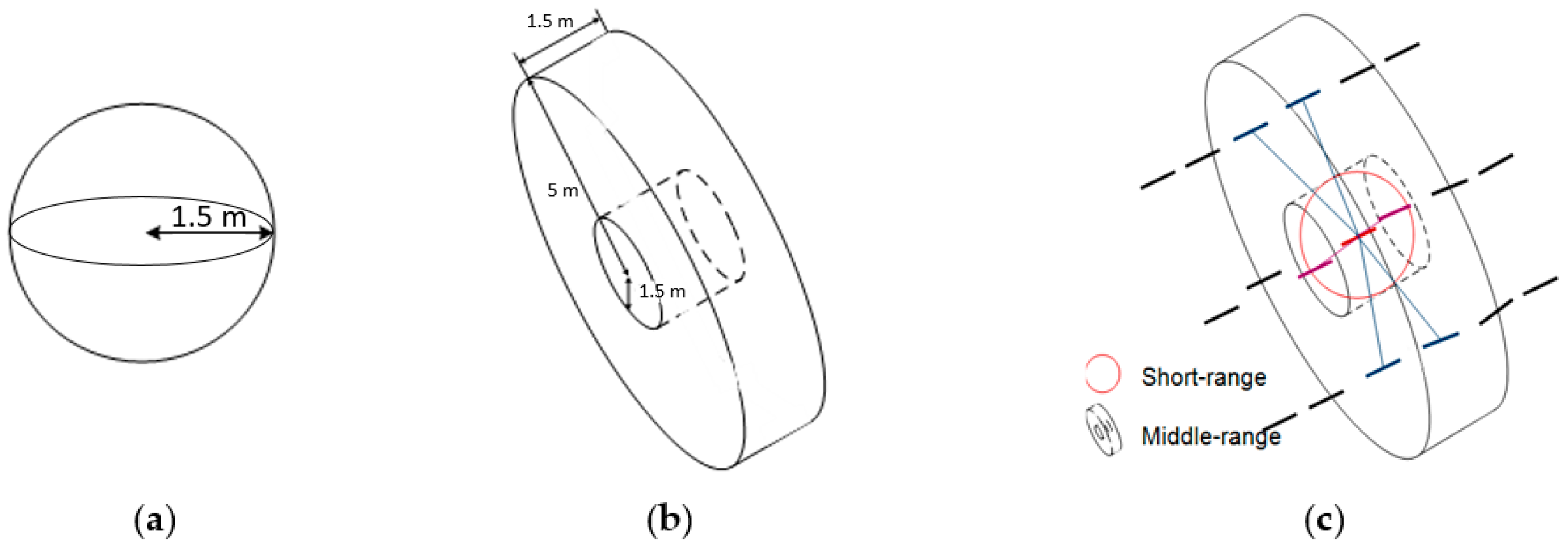
Neighboring systems: (a) for short-range graph; (b) for long-range graph; and (c) combined neighboring systems.
Remotesensing 08 01008 g001
Figure 2. 
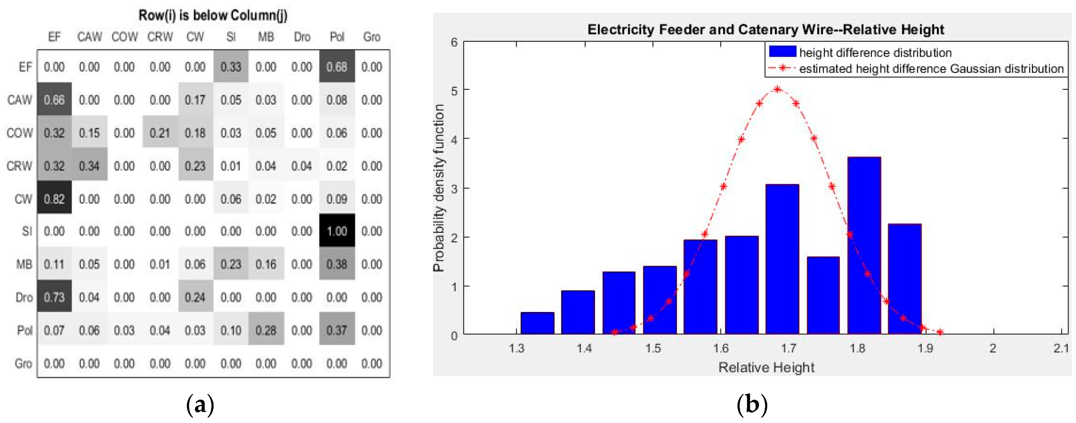
Prior and likelihood estimation of the vertical long-range pairwise potential: (a) look-up table where row i is below column j; and (b) probability density distribution of the height difference (red curve: estimated Gaussian distribution learned from the training data).
Remotesensing 08 01008 g002
Figure 3. 
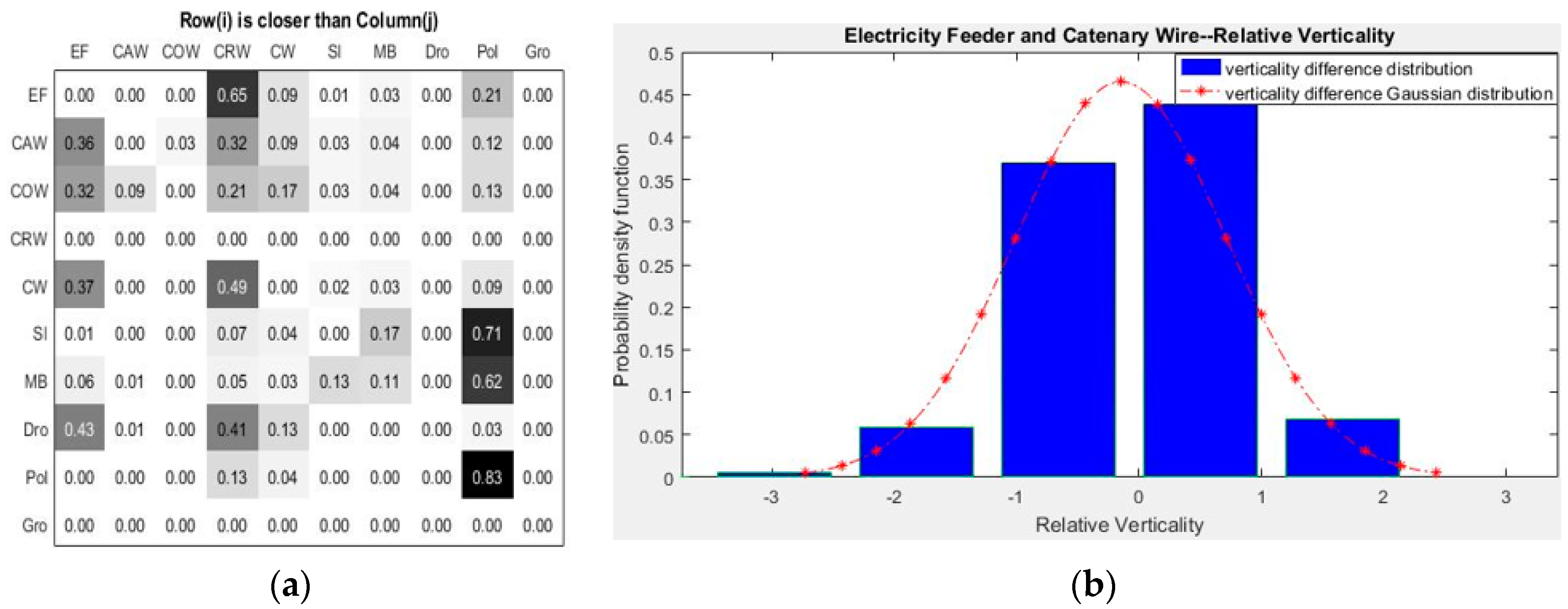
Prior and likelihood estimation of the horizontal long-range pairwise potential: (a) look-up table where row i is closer to the railway than column j; and (b) probability density distribution of the verticality difference (red curve: estimated Gaussian distribution learned from training data).
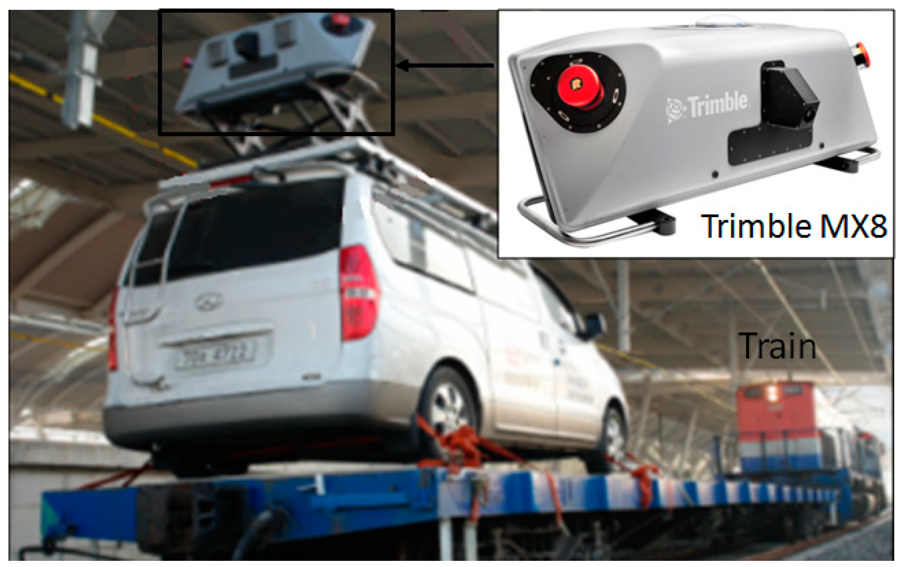
Remotesensing 08 01008 g003
Figure 4. Trimble MX8 mounted on a train.
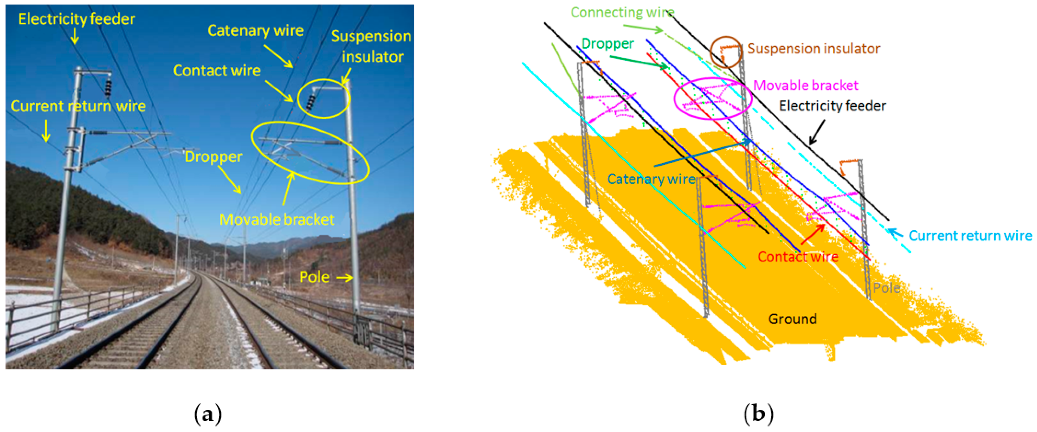
Remotesensing 08 01008 g004
Figure 5. Electrification system configuration and 10 object classes of the Honam high-speed railway illustrated in: (a) a photograph; and (b) Mobile Laser Scanning (MLS) data.
Remotesensing 08 01008 g005
Figure 6. 
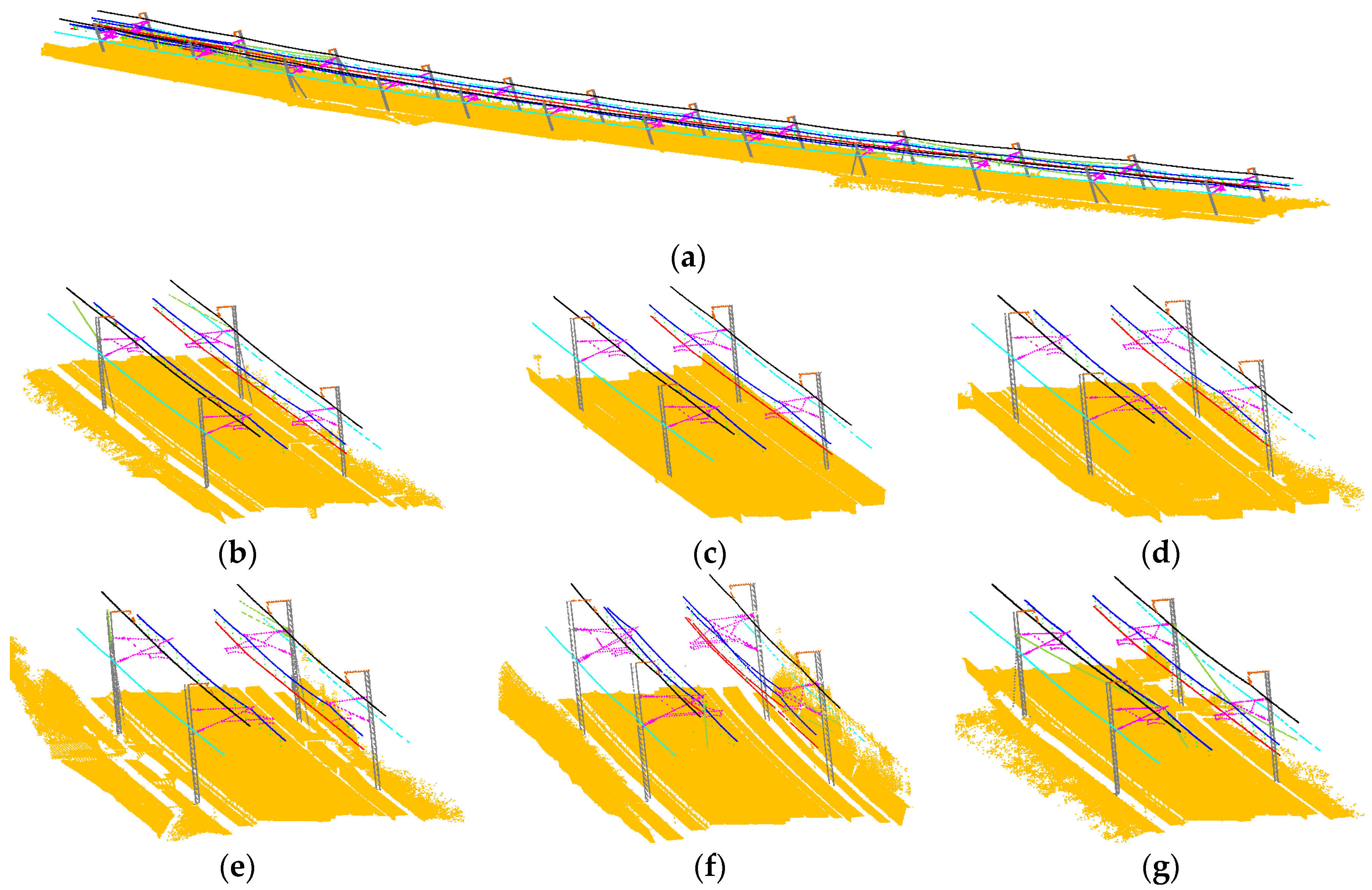
Manually-classified reference data: (a) entire region; and (bg) six sub-regions (different colors represent different classes).
Remotesensing 08 01008 g006
Figure 7. Example of voxelization and line extraction: (a) input MLS data and rail vectors, (b) voxelization; and (c) extracted lines.
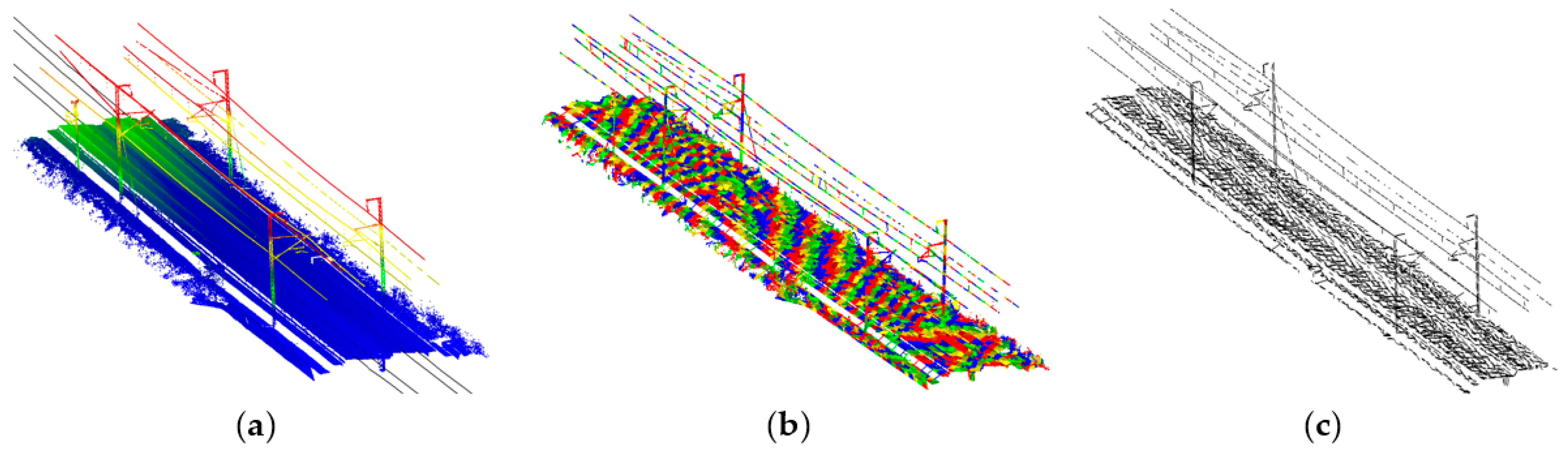
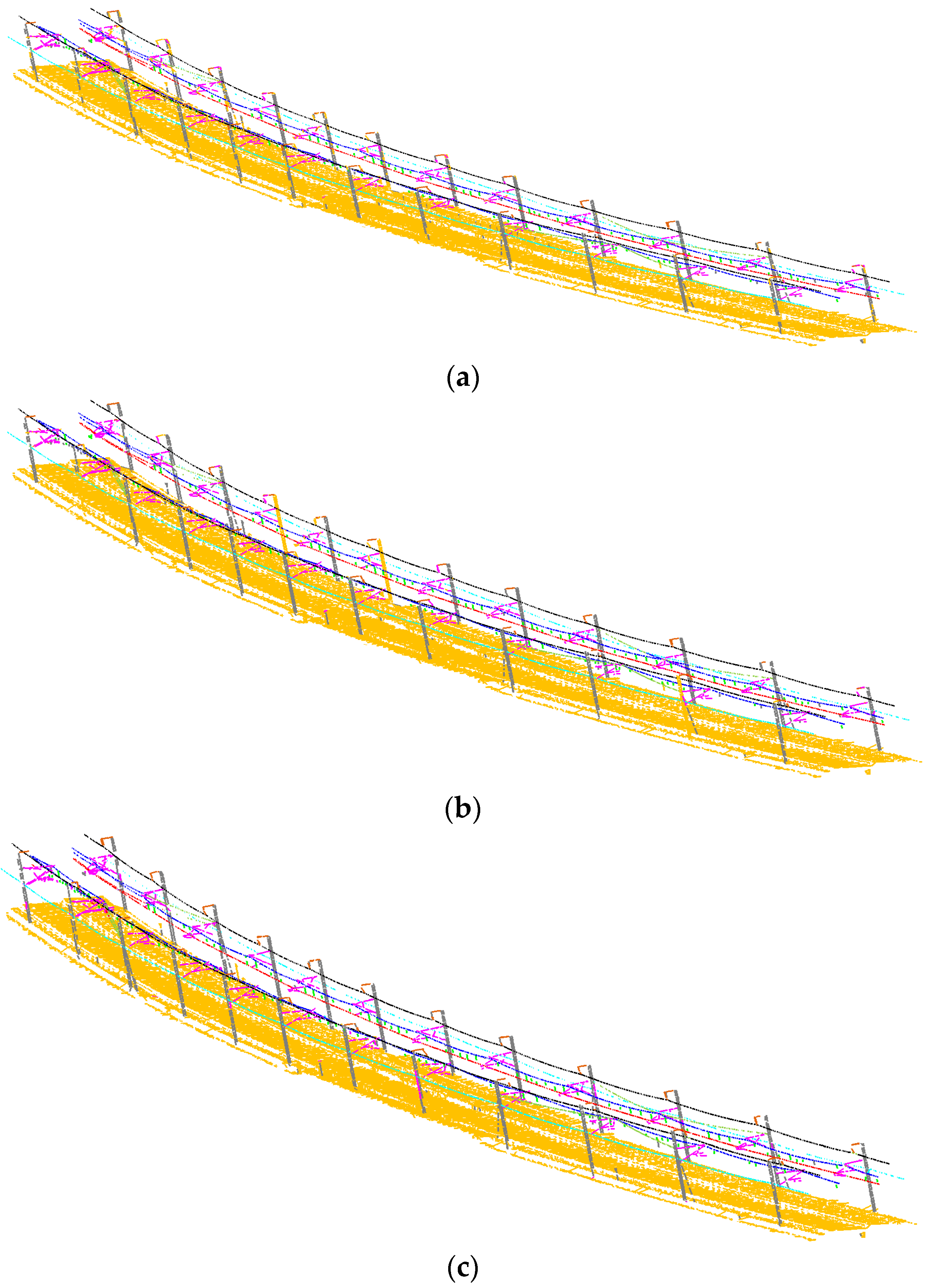
Remotesensing 08 01008 g007
Figure 8. Classification results produced over the entire railway test scene by: (a) SVM; (b) short-range Conditional Random Field (CRF); and (c) multi-range CRF; electricity feeder (black), catenary wire (blue), contact wire (red), current return wire (sky blue), connecting wire (dark green), suspension insulator (brown), movable bracket (magenta), dropper (green), pole (grey) and ground (orange).
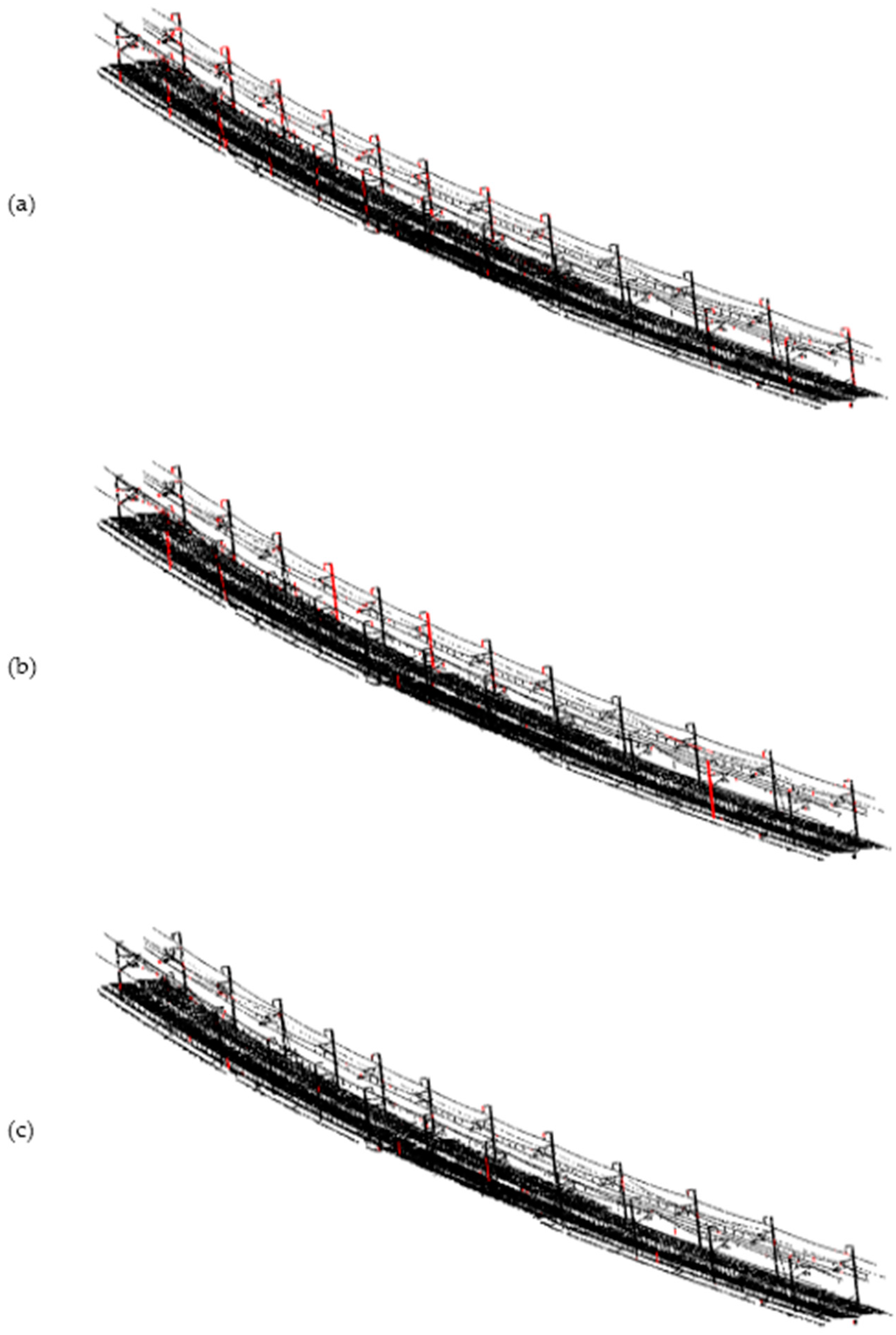
Remotesensing 08 01008 g008
Figure 9. Classification errors (false positive and false negative) highlighted with red colors produced by: (a) SVM; (b) short-range CRF; and (c) multi-range CRF.
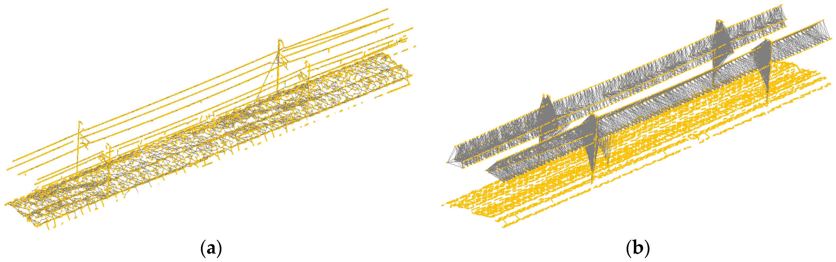
Remotesensing 08 01008 g009
Figure 10. Examples of the (a) short-range graph; and (b) long-range graph.
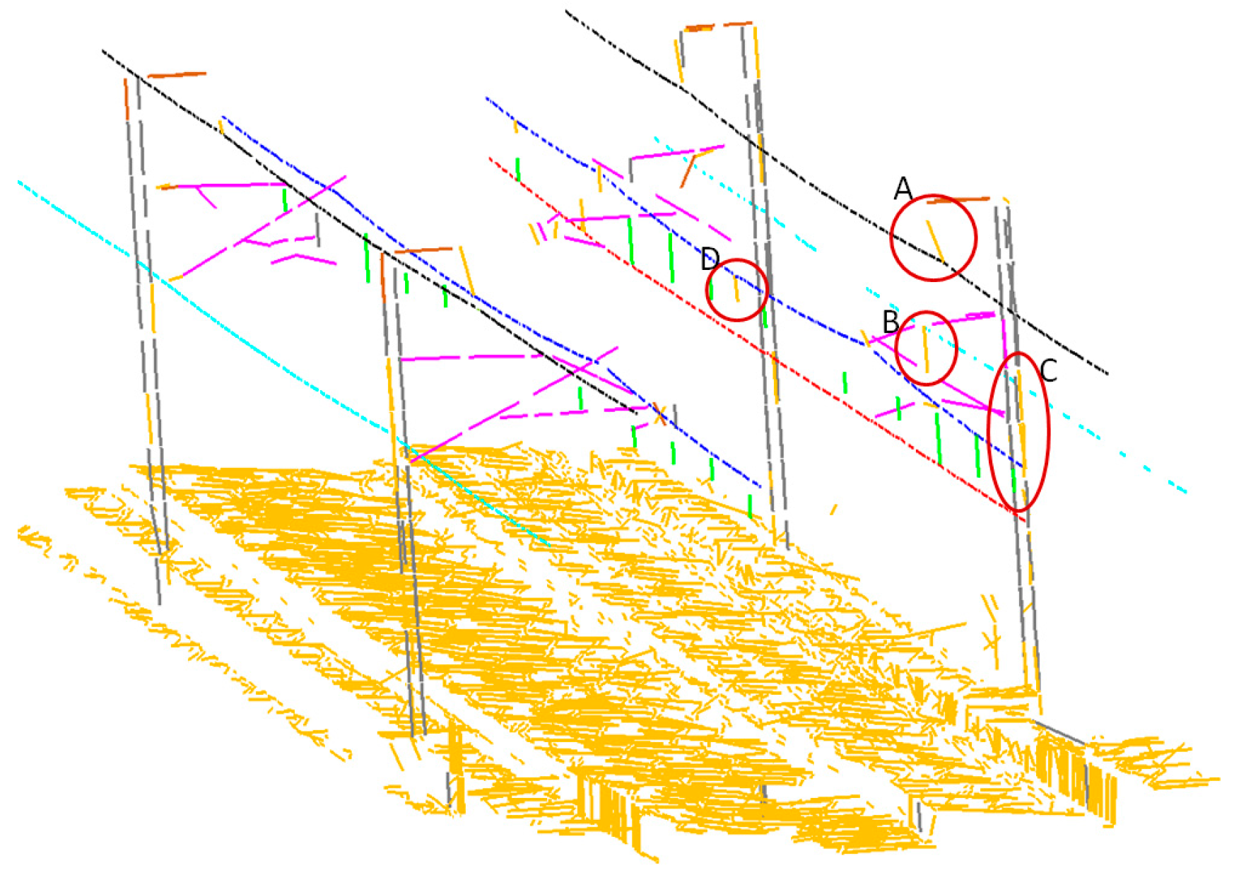
Remotesensing 08 01008 g010
Figure 11. Examples of errors caused by SVM: (A) the suspension insulator in the reference was classified to ground; (B) the movable bracket in the reference was classified to ground; (C) the pole was classified to ground; and (D) the dropper in the reference was classified to pole.
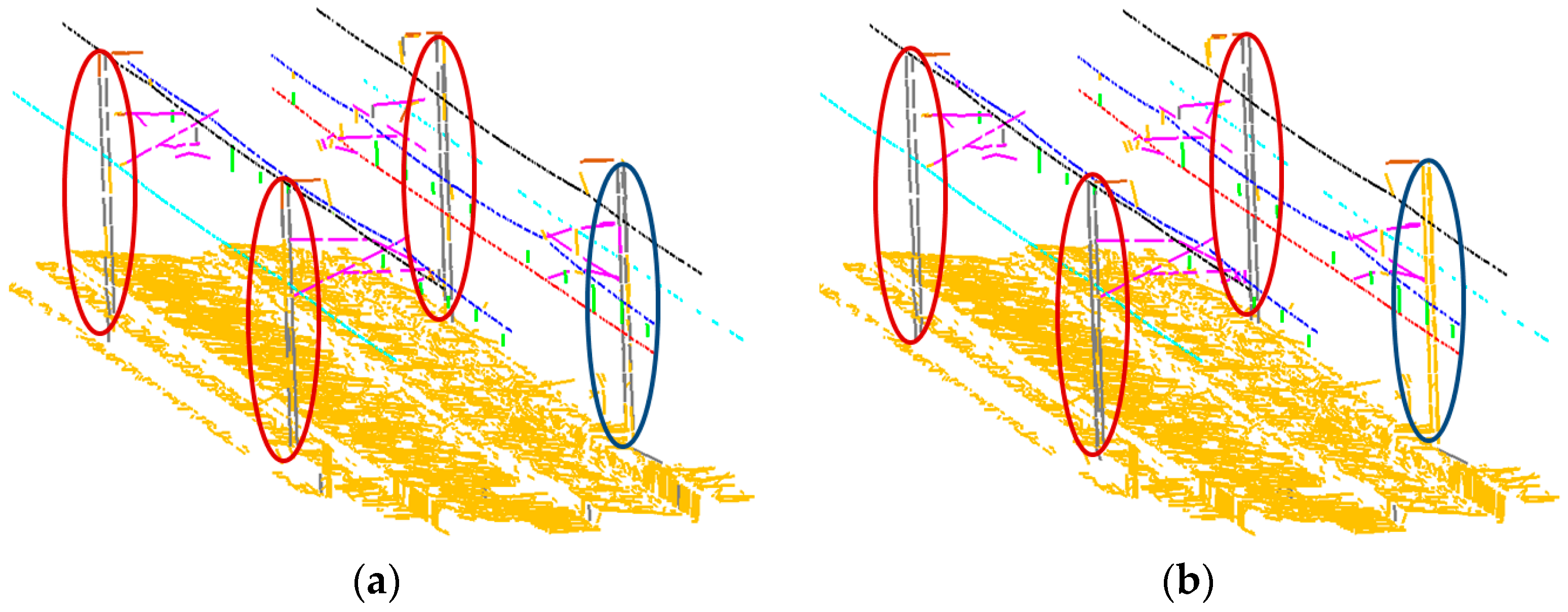
Remotesensing 08 01008 g011
Figure 12. Effects on short-range CRF: (a) SVM results; and (b) short-range CRF results.
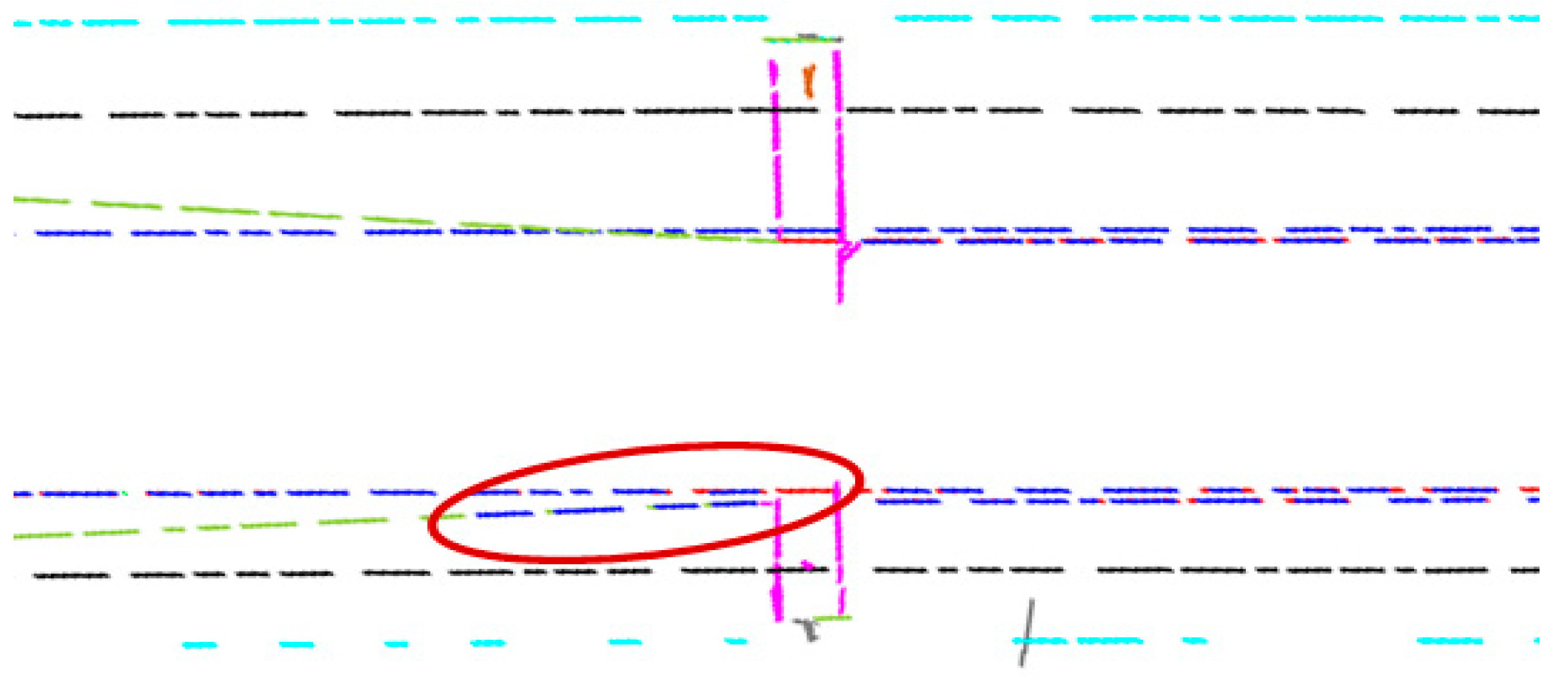
Remotesensing 08 01008 g012
Figure 13. An example of errors produced over connecting wires (dark green) shown in the top view (sky blue: current return wire; black: electricity feeder; blue: catenary wire; red: contact wire; brown: suspension insulator; magenta: movable bracket; grey: pole).
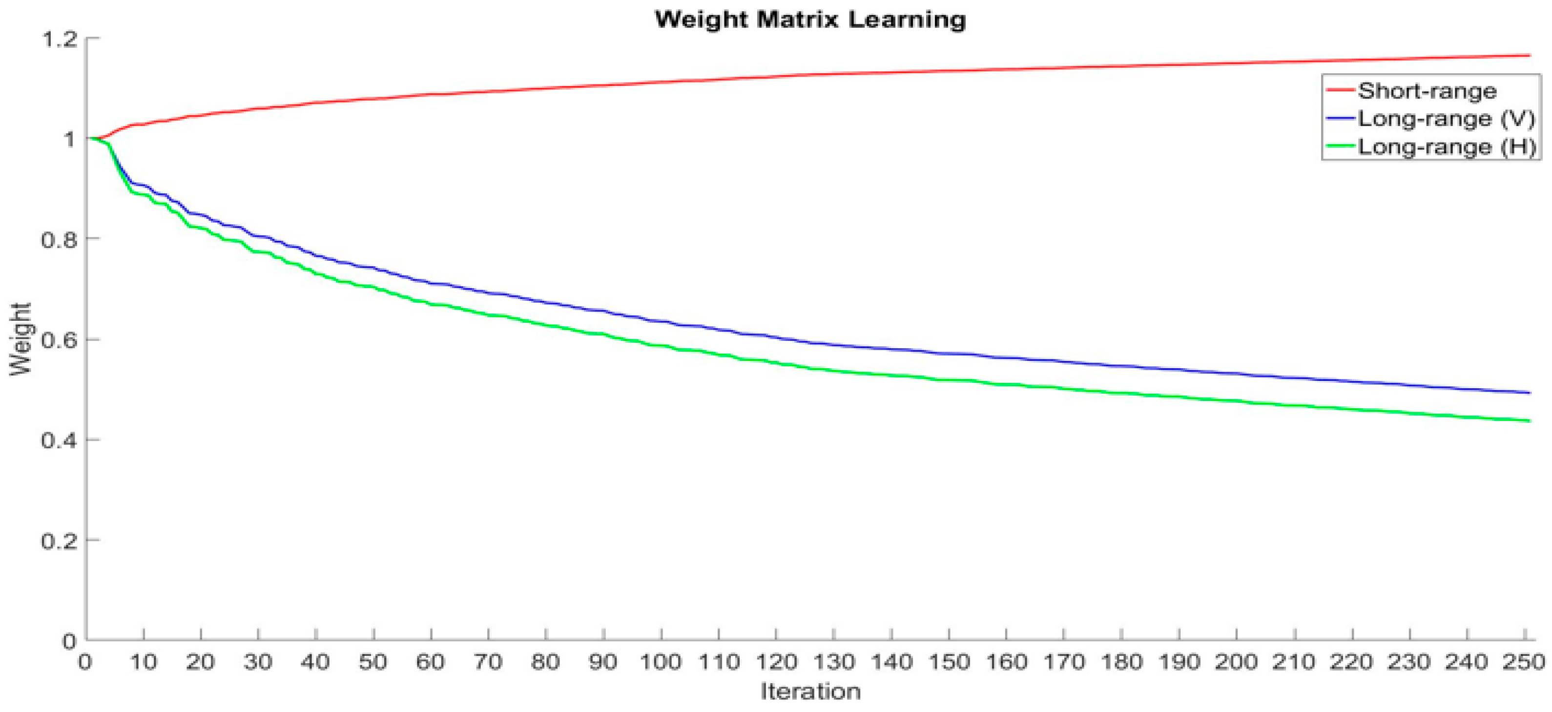
Remotesensing 08 01008 g013
Figure 14. Weight learning of the multi-range CRF model using the SGD algorithm.
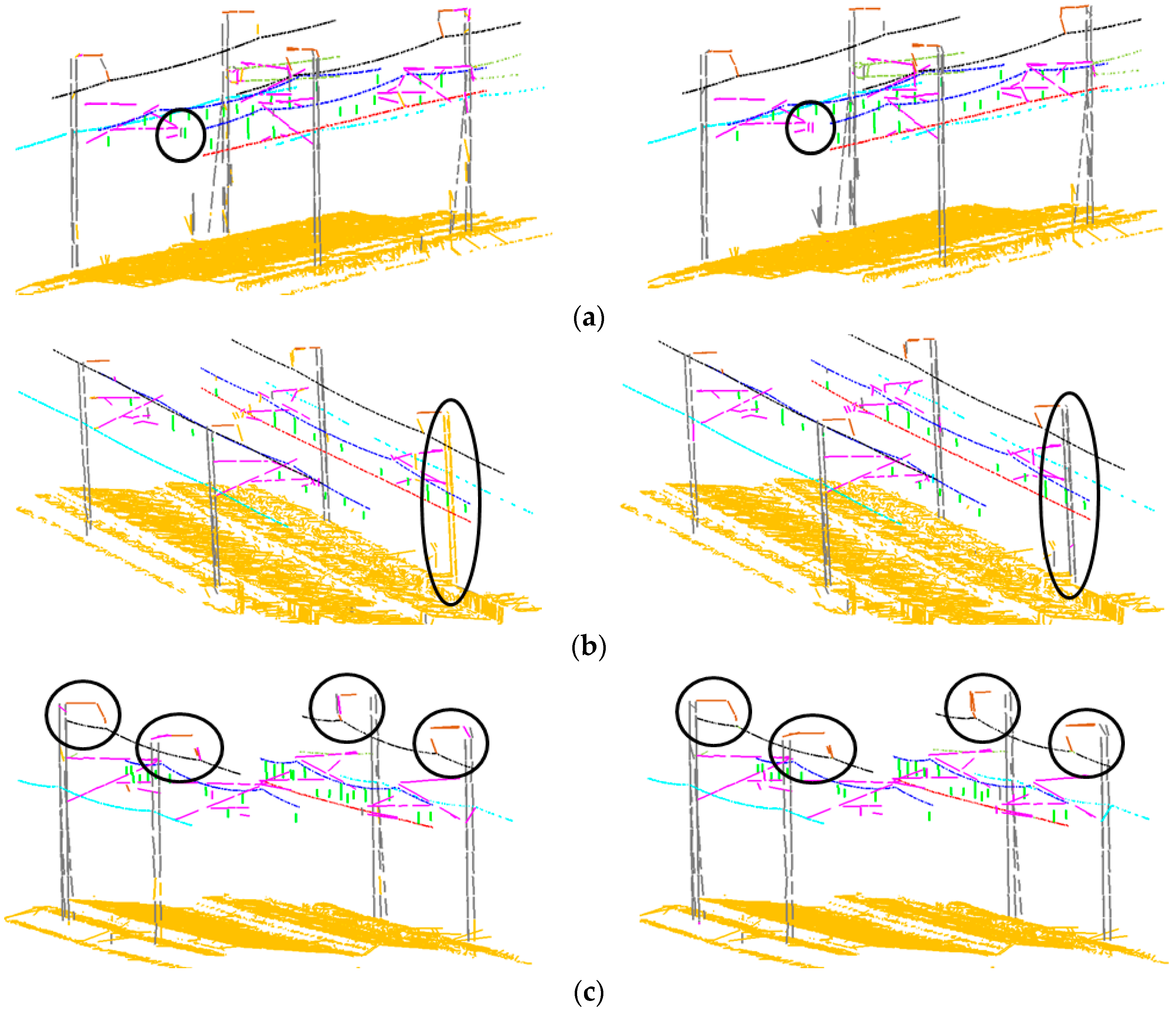
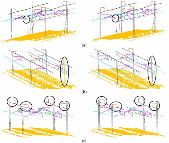
Remotesensing 08 01008 g014
Figure 15. Visualization of label transitions: (a) the dropper in the SVM results (left) was classified to movable bracket in the integrated CRF model (right); (b) the ground in the short-range CRF (left) was classified to pole in the integrated CRF model (right); (c) the suspension insulators were well rectified in the integrated CRF model (right).
Remotesensing 08 01008 g015
Figure 16. 
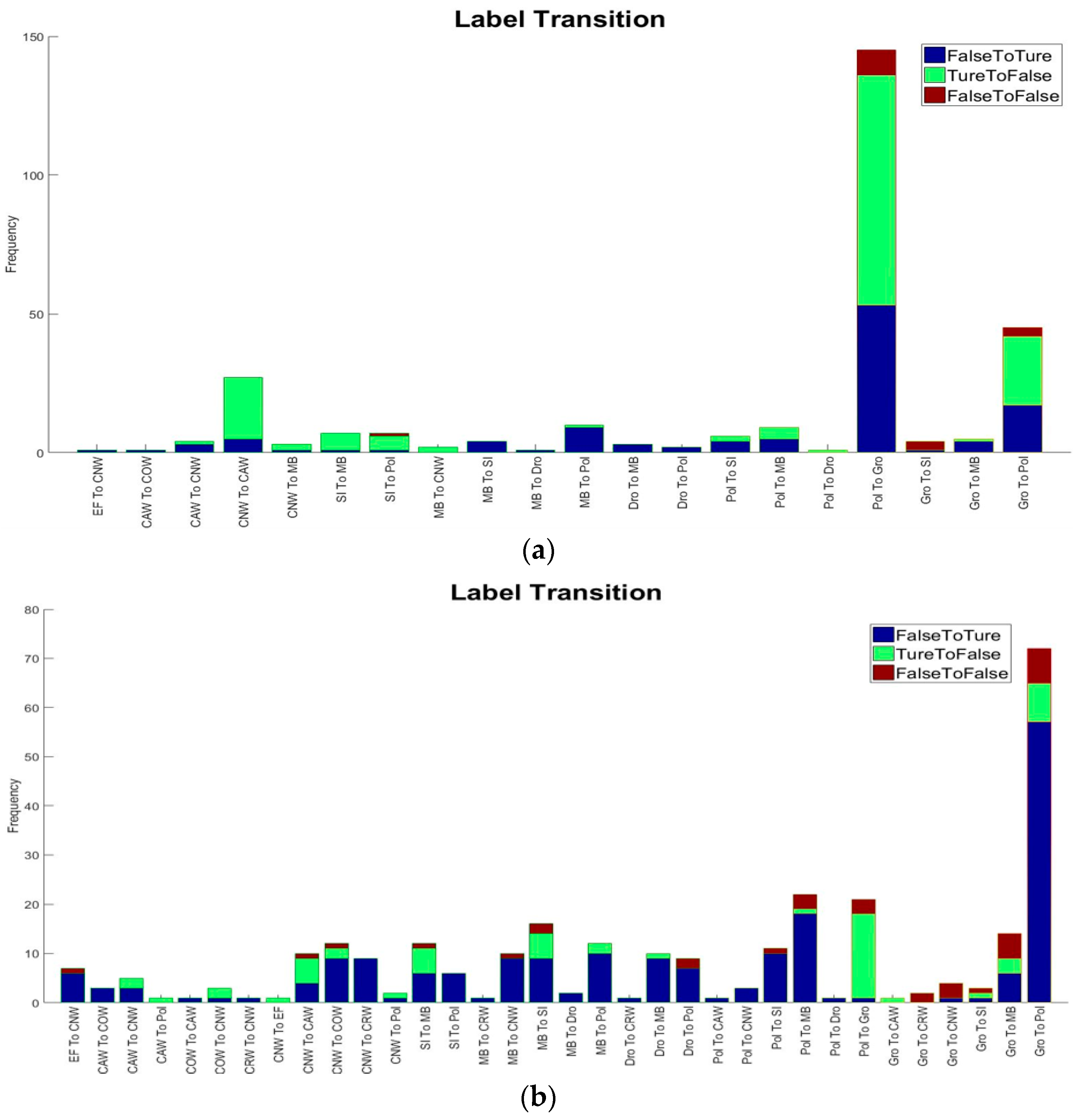
Label transitions: (a) from SVM to short-range CRF; and (b) from SVM to multi-range CRF: EF (electricity feeder), CAW (catenary wire), COW (contact wire), CRW (current return wire), CNW (connecting wire), SI (suspension insulator), MB (movable bracket), Dro (dropper), Pol (pole) and Gro (ground).
Remotesensing 08 01008 g016
Table 1. Specifications of the Trimble MX8 system [31].
ParameterValues
Accuracy10 mm
Precision5 mm
Maximum effective measurement rate600,000 points/second
Line scan speedUp to 200 lines/second
Echo signal intensityHigh resolution 16-bit intensity
RangeUp to 500 m
Table 2. Extracted lines for each sub-region.
Sub-RegionRegion 1Region 2Region 3Region 4Region 5Region 6
# of extracted lines432744273783409147304762
Table 3. Edge number of different models in different sub-regions.
Edge NumberRegion 1Region 2Region 3Region 4Region 5Region 6
# of short-range edges696778446671765794608469
# of long-range edges 700075576764772811,3318005
Table 4. Confusion matrix for SVM results: electricity feeder (EF), catenary wire (CAW), contact wire (COW), current return wire (CRW), connecting wire (CNW), suspension insulator (SI), movable bracket (MB), dropper (Dro), pole (Pole) and ground (Gro).
ClassifiedRecall (%)
EFCAWCOWCRWCNWSIMBDroPoleGro
ReferenceEF124900020000099.84
CAW013650040200099.56
COW01687020100199.28
CRW00097000100099.90
CNW080037201206692.08
SI000007315016566.97
MB11067123751281186.61
Dro00000041345193.06
Pole000026916786988.63
Gro000000204619,93299.76
Precision (%)99.9299.2710099.3895.6380.2289.0791.1689.3399.5498.91
Table 5. Confusion matrix for short-range CRF: electricity feeder (EF), catenary wire (CAW), contact wire (COW), current return wire (CRW), connecting wire (CNW), suspension insulator (SI), movable bracket (MB), dropper (Dro), pole (Pole) and ground (Gro).
ClassifiedRecall (%)
EFCAWCOWCRWCNWSIMBDroPoleGro
ReferenceEF124900020000099.84
CAW013650040200099.56
COW00688020100199.42
CRW00097000100099.90
CNW0300034901704486.39
SI000008314011176.15
MB020678384813588.68
Dro00000031365094.44
Pole0000206061214580.00
Gro000000301719,96099.90
Precision (%)10097.7110099.3995.3691.2189.1094.4492.4599.2298.76
Table 6. Confusion matrix for integrated CRF: electricity feeder (EF), catenary wire (CAW), contact wire (COW), current return wire (CRW), connecting wire (CNW), suspension insulator (SI), movable bracket (MB), dropper (Dro), pole (Pole) and ground (Gro).
ClassifiedRecall (%)
EFCAWCOWCRWCNWSIMBDroPoleGro
ReferenceEF124400070000099.44
CAW013660020102099.64
COW02684030102098.84
CRW00097010000099.90
CNW081473700104091.58
SI00000102007093.58
MB030114041104094.92
Dro00000061308090.28
Pole000011160747097.65
Gro000000202819,95099.85
Precision (%)10099.0697.9998.1895.3699.0393.8410093.1410099.44
Table 7. A summary of the classification performance achieved by three classifiers (unit: %).
Class(a) SVM(b) Short-Range CRF(c) Multi-Range CRF
RecallPrecisionF1RecallPrecisionF1RecallPrecisionF1
EF99.8499.9299.8899.8410099.9299.4410099.72
CAW99.5699.2799.4199.5697.7198.6399.6499.0699.35
COW99.2810099.6399.4210099.7198.8497.9998.42
CRW99.9099.3899.6499.9099.3999.6499.9098.1899.03
CNW92.0895.6393.8286.3995.3690.6591.5895.3693.43
SI66.9780.2273.0076.1591.2183.0093.5899.0396.23
MB86.6189.0787.8288.6889.1088.8994.9293.8494.37
Dro93.0691.1692.0994.4494.4494.4490.2810094.89
Pole88.6389.3388.9780.0092.4585.7797.6593.1495.34
Gro99.7699.5499.6499.9099.2299.5699.8510099.92
Average92.5794.3593.3992.4395.8994.0296.5797.6697.07
Table 8. The comparison of three different classifiers (unit: %): (a) short-range CRF—SVM; (b) multi-range CRF—SVM; and (c) multi-range CRF—short-range CRF.
Class(a) Short-Range—SVM(b) Multi-Range—SVM(c) Multi-Range—Short-Range
RecallPrecisionF1RecallPrecisionF1RecallPrecisionF1
EF0+0.08+0.04−0.40+0.08−0.16−0.40−0.2
CAW0−1.56−0.78+0.08−0.21−0.06+0.08+1.35+0.72
COW+0.140+0.08−0.44−2.01−1.21−0.58−2.01−1.29
CRW0+0.0100−1.20−0.610−1.21−0.61
CNW−5.69−0.27−3.17−0.50−0.27−0.39+5.190+2.78
SI+9.18+10.99+10.00+26.61+18.81+23.32+17.43+7.82+13.23
MB+2.07+0.03+1.07+8.31+4.77+6.55+6.24+4.74+5.48
Dro+1.38+3.28+2.35−2.78+8.84+2.80−4.16+5.56+0.45
Pole−8.63+3.12−3.20+9.02+3.81+6.37+17.65+0.69+9.57
Gro+0.14−0.32−0.08+0.09+0.46+0.28−0.05+0.78+0.36
Average−0.14+1.54+1.54+4.00+3.31+3.68+4.14+1.77+3.05
Table 9. Comparison of accuracy and precision between [2] and the proposed multi-range CRF.
Class(a) Results from [2](b) Multi-Range CRF(b)–(a)
AccuracyPrecisionAccuracyPrecisionAccuracyPrecision
Catenary wire96.9295.8799.9399.06+3.013.19
Contact wire97.6696.0299.9297.99+2.261.97
Current return wire94.7299.6399.9398.18+5.21−1.45
Movable bracket91.2397.4399.8193.84+8.58−3.59
Pole99.4295.1799.7293.14+0.30−2.03
Average95.9996.8299.8696.44+3.87−0.38

