The Impact of Inter-Modulation Components on Interferometric GNSS-Reflectometry

Abstract

The interferometric Global Navigation Satellite System Reflectometry (iGNSS-R) exploits the full spectrum of the transmitted GNSS signal to improve the ranging performance for sea surface height applications. The Inter-Modulation (IM) component of the GNSS signals is an additional component that keeps the power envelope of the composite signals constant. This extra component has been neglected in previous studies on iGNSS-R, in both modelling and instrumentation. This letter takes the GPS L1 signal as an example to analyse the impact of the IM component on iGNSS-R ocean altimetry, including signal-to-noise ratio, the altimetric sensitivity and the final altimetric precision. Analytical results show that previous estimates of the final altimetric precision were underestimated by a factor of $1.5\sim 1.7$ due to the negligence of the IM component, which should be taken into account in proper design of the future spaceborne iGNSS-R altimetry missions.

1. Introduction

Since the proposal of the PAssive Reflectometry and Interferometry System (PARIS) concept in 1993 [1], the reflection of Global Navigation Satellite System (GNSS) signals has been a option for various Earth surface remote sensing applications. This technique, also known as GNSS-Reflectometry (GNSS-R), can provide a dense spatial and temporal sampling capability over the Earth surface in a low-cost way. During the past two decades, several theoretical and experimental studies have been performed to demonstrate the feasibility of ocean altimetry using reflected GNSS signals, e.g., in [2,3,4,5,6,7,8,9], and several studies have been performed on scatterometric applications, such as sea surface wind, sea ice and soil moisture. A comprehensive tutorial of GNSS-R technique and its applications can be found in [10].

As in traditional radar altimeters (RA), the delay of the return echo from the sea surface is the primary observable in GNSS-R altimetry, and its accuracy increases with the signal-to-noise ratio (SNR) and the bandwidth of the transmitted signal. Unfortunately, the transmitted power of GNSS signals is relatively low and the open-access signals have much narrower bandwidths than signals in traditional RA, which lead to the lower altimeric performance of the conventional GNSS-R approach (cGNSS-R). To overcome the bandwidth limitation, some alternative approaches have been proposed to exploit the wideband encrypted signals, such as those presented in [11,12], known as reconstructed GNSS-R (rGNSS-R), and in [13], known as interferometric GNSS-R (iGNSS-R). Nevertheless, any of the aforementioned GNSS-R techniques operate at much lower bandwidths (2∼40 MHz) than that in traditional RAs (∼320 MHz), resulting in very different ranging precision.

The iGNSS-R technique was proposed in [1] and discussed in detail in [13] for the ESA-proposed PARIS In-orbit Demonstrator (PARIS IoD) mission. In addition, it is also considered in the GNSS Reflectometry, Radio Occultation and Scatterometry candidate experiment aboard the International Space Station (GEROS-ISS) [14]. In iGNSS-R, the reflected signals are directly correlated against the direct signals, i.e., the signals that arrive through the line-of-sight path (see Figure 1), instead of a locally-generated clean replica as it is the case in cGNSS-R. It allows to extract information from the full spectrum of the transmitted GNSS signals, thus resulting in a sharper auto-correlation function (ACF) and improving the altimetric precision. Results from airborne experiments [15] show at least two-fold improvement in altimetric precision compared to the clean replica method, further theoretical analysis [16,17,18,19] predicts an improvement of the ranging precision by a factor of $2\sim 3$.

The modernized GNSS signals, such as GPS L1 signals transmitted by all block IIR-M and later design satellites, Galileo signals transmitted at E1/E6 bands and BeiDou signals transmitted at B1/B3 bands, are composed of several components modulated on to the same carrier to provide different navigation services (e.g., C/A (Coarse Acquisition) code, P (Precise) code and M (Military) code signals at GPS L1 band). In addition to these, byproduct signal components of using interplex modulation [20], known as Inter-Modulation (IM) components, are transmitted to combine all signal components on the same carrier and maintain constant envelope and saturation of the high-power amplifier. In general, the IM component is neglected in cGNSS-R and rGNSS-R as there is no correlation between them and the desired signal codes. Instead, by it’s nature the interferometric processing exploits all the signals collected from the up- and down-looking antennas, the IM component in the direct and reflected chains are also cross-correlated together with the desired signals, thus impacting the characteristics of the interferometric waveform. However, the presence of the IM component in the modulation scheme is not presented in any official Open Service Signal-In-Space Interface Control Documents (OS SIS ICD), and its impact on iGNSS-R has been neglected in previous studies.

This paper fixes the omission of the IM component from previous studies on iGNSS-R and investigates the impact of the GPS L1 IM components on iGNSS-R ocean altimetry performance. In Section 2, the GPS L1 signal is taken as an example to introduce the theoretical basis of the IM component and revise the ACF of the GPS L1 composite signal as used in [13] for modern GNSS signals. After verifying the existence of this component with an experimental dataset, the effects of the IM component to ocean altimetry are studied analytically, including the SNR, the altimetric sensitivity, as well as the final altimetric precision, in Section 3.

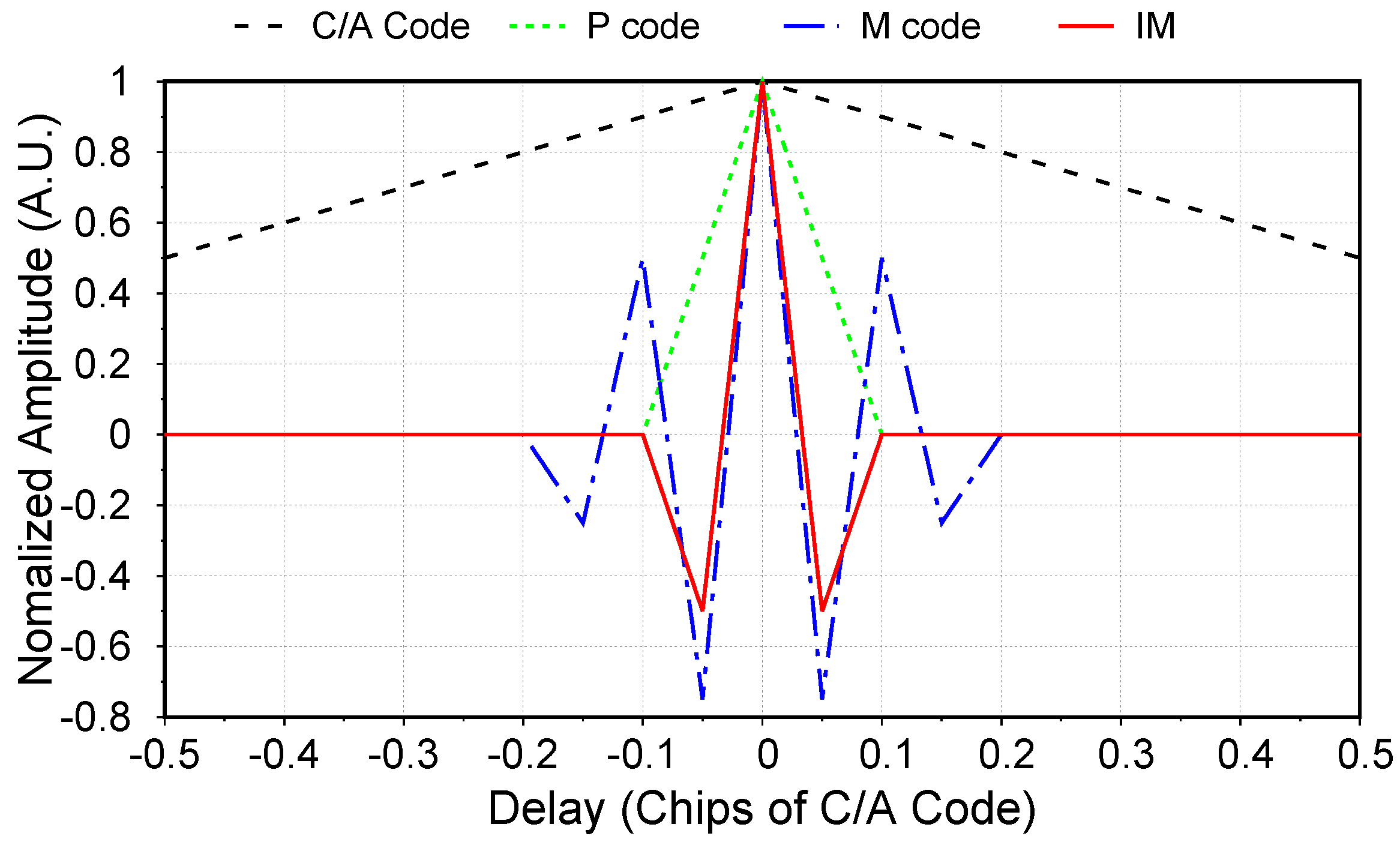
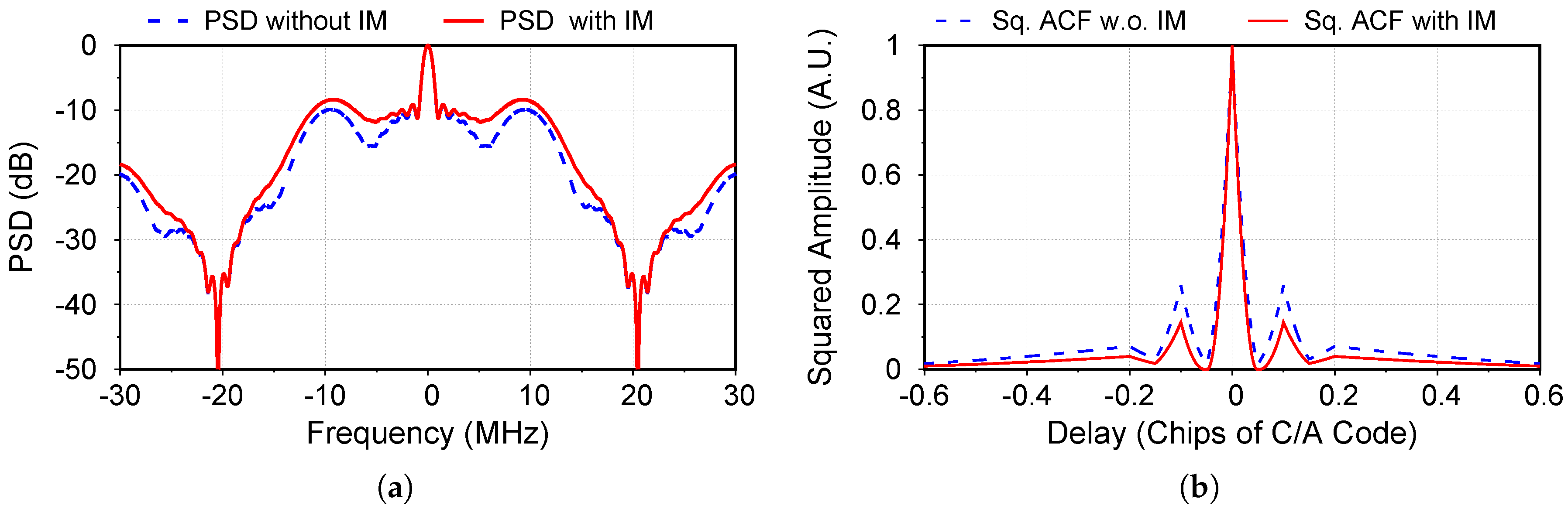
2. Characteristics of the Multiplexed Signals

Because of the limited availability of the spectrum allocated for navigation systems, the modernized GNSS signals are composed of several components multiplexed on the same carrier using the Coherent Adaptive Subcarrier Modulation (CASM), a multichannel modulation scheme also known as tricode hexaphase modulation or interplex modulation [20,21]. This technique was proposed to keep the power envelope of the transmitted signals constant, i.e., the total transmitted power does not vary over time. It is also important to allow the use of a high-power amplifier operating close to saturation with limited signal distortion. However, this technique yields a byproduct signal that is not useful in the navigation applications.

Taking the GPS L1 band as an example, the modernized GPS satellites (GPS IIR-M and II-R) transmit three different navigation signals: the C/A, P and M code components. The CASM modulation places the P and the M codes in the in-phase component (I) and the C/A code in the quadrature component (Q) with the IM component. The transmitted L1 signal at baseband could be expressed as [22]

$$\begin{array}{cc}\hfill s_{L1}\left(t\right)=& \sqrt{2}\left(\sqrt{P_P}{s}_P\left(t\right)-\sqrt{P_M}{s}_M\left(t\right)\right)+\hfill \\ & j\sqrt{2}\left(\sqrt{P_{CA}}{s}_{CA}\left(t\right)+\sqrt{P_{IM}}{s}_{IM}\left(t\right)\right)\hfill \end{array}$$

(1)

in which the subscripts denote the signal components of P, M, C/A and IM respectively, $s_{*}\left(t\right)$ are the spreading code modulated baseband navigation signals, $P_{*}$ are the powers of each signal component and the IM component is the product of the three useful components as $s_{IM}\left(t\right)=s_{CA}\left(t\right)s_P\left(t\right)s_M\left(t\right)$. Since the IM component is not correlated with the other signal components, i.e., $〈s_{IM}\left(t\right)s_X\left(t\right)〉=0$, it can be neglected in general GNSS signal processing for navigation, as well as in the cGNSS-R and rGNSS-R approaches.

In modernized GNSS systems, the Binary Phase-Shift Keying (BPSK) and Binary Offset Carrier (BOC) modulations are used in different navigation signals. The general expression for BPSK and BOC modulations could be written as $\mathrm{BPSK}\left(n\right)$ and $\mathrm{BOC}(n,m)$, in which n and m refer to the code chipping rate of $n\times 1.023\mathrm{MHz}$ and the subcarrier frequency of $m\times 1.023\mathrm{MHz}$. Thus, the C/A code, P code and M code could be expressed as BPSK(1), BPSK(10) and BOC(10, 5) respectively, and the IM component as BOC(10, 10) [23]. Figure 2 summarizes the ACFs of the different signal components in the GPS modernized L1 band.

In [22], the GPS L1 band signal from GPS Block IIR-M #6 (PRN 07) satellite was analysed using a high gain antenna and the relative power of each signal component was estimated. The main characteristics of these signal components are summarized in

Table 1. Main characteristics of the signal components transmitted by GPS Block IIR-M satellites at L1 band computed from [22].

Signal	Carrier Phase	Modulation	Percentage of Power
C/A code	Q	BPSK(1)	25%
P code	I	BPSK(10)	18.75%
M code	I	BOC(10, 5)	31.25%
IM	Q	BOC(10, 10)	25%

. In Figure 3, the ideal power spectral density (PSD) $S_{\mathrm{L}1}\left(f\right)$ and the Woodward Ambiguity Function (WAF), i.e., the squared ACF of the fully composite GPS L1 signal ${\mathsf{\Lambda }}^2\left(\tau \right)$, are compared against those of its ranging components, i.e., the composite of C/A, P and M codes as in previous studies. As expected, the wide band and the split-spectrum properties of the IM component increase the spectral energy further away from the carrier frequency, therefore sharpening the main lobe and reducing the side lobes of the ACF.

To further validate the existence of the IM component and its effect on the iGNSS-R waveform, the raw samples collected on 3 December 2015 during an airborne experiment over the Baltic Sea were processed. A new instrument, known as the Software PARIS Interferometric Receiver (SPIR) [24], was used in this campaign. Thanks to the flexibility of the SPIR instrument, the up-looking antenna array (with 8 elements) can be divided into two independent sub-arrays with four antenna elements each. Similar to the partial interferometric processing method in [25], the in-phase and quadrature components of the beamformed signals are separated through the carrier phase tracking loop. By cross-correlating the extracted signal components from both sub-arrays, the waveforms of the GPS L1 in-phase and quadrature components (WF-I and WF-Q) from PRN01 have been produced separately, as shown in Figure 4. The existence of a wideband component in the quadrature component waveform can be noticed by the sharp ACF, compared to a pure C/A code ACF (see Figure 4).

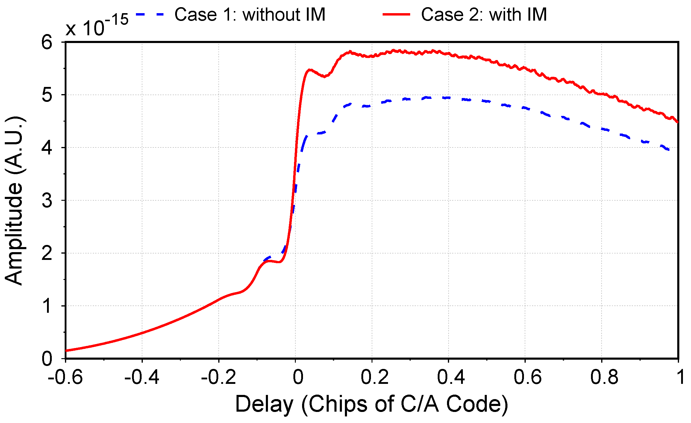
3. Impact on iGNSS-R Altimetric Performance

With the existence of the IM component in iGNSS-R waveform verified, we analyzed the impact of the IM component and revised the iGNSS-R altimetric performance of [13] by using the PSD and WAF models derived in the previous section. In this analysis, a spaceborne scenario with a height of 600 km (as is intended for the PARIS-IoD mission [13]) is considered.

Table 2. Parameters For Simulation.

Parameter			Value	Unit
Orbit Altitude			600	Km
Incidence Angle at the SP			15	deg
Wind Speed at 10 m (U10)			7	m/s
Antenna Directivity at Nadir			22.6	dB
Receiver Bandwidth			12	MHz
Coherent Integration Time			1	ms

shows the main parameters of our analysis, which focuses on the comparison of two cases:

-

Case 1: considering only the ranging components, i.e., the composite of the C/A, P and M codes as in previous studies,

-

Case 2: considering the fully composite signal including both the ranging, as well as the extra IM component.

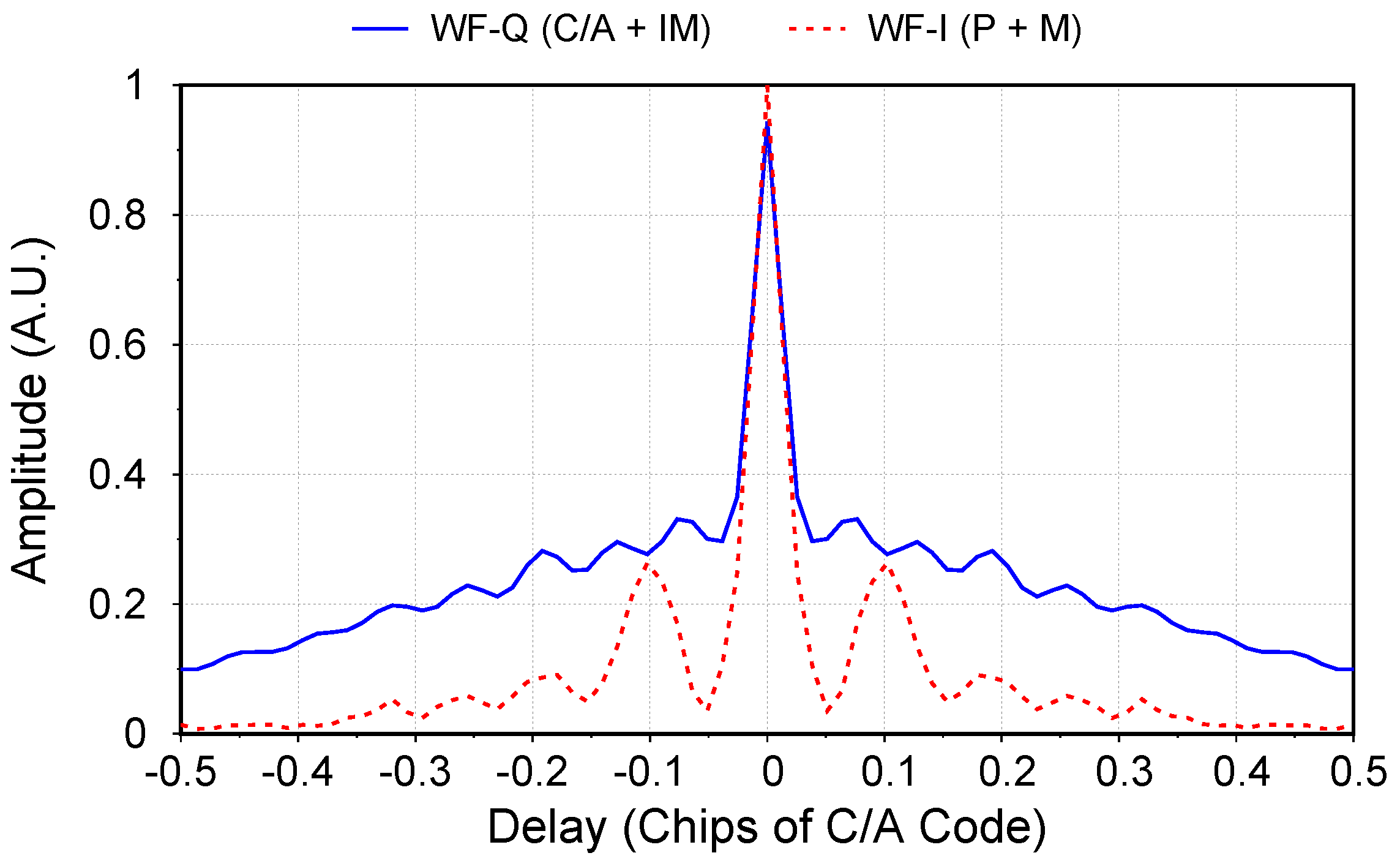
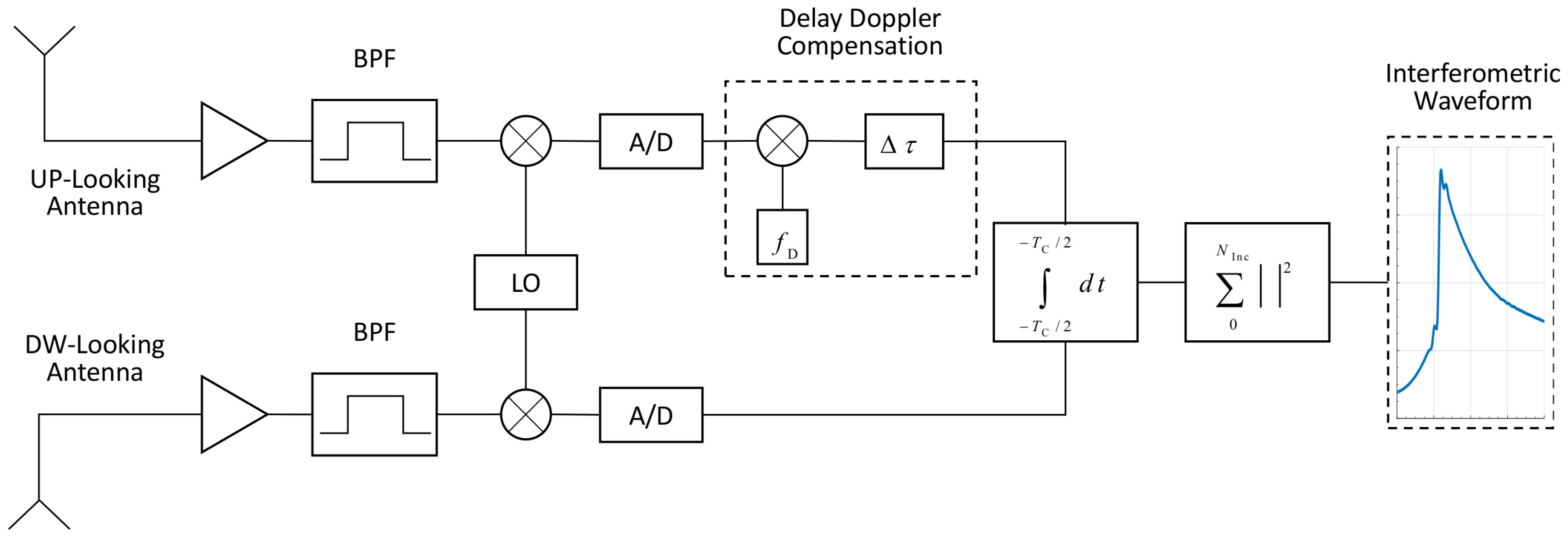
3.1. Waveform Model

The ocean reflected GNSS signal can be modelled as the sum of the returns from many scattering elements of the sea surface. Models of GNSS waveforms for reflections over the ocean are derived in [13,26,27]. After simplification, the useful signal component in the power waveform can be expressed as the convolution product

$$\begin{array}{c}\hfill \langle Z_S\left(\tau \right)\rangle =W\left(\tau \right)\otimes {\mathsf{\Lambda }}_B^2\left(\tau \right)\end{array}$$

(2)

where the weight function $W\left(\tau \right)$, known as the flat surface impulse response in conventional radar altimetry, represents the contribution to the waveform of the points with a delay τ and ${\mathsf{\Lambda }}_B\left(·\right)$ is the band-limited ACF of the GNSS signal.

In order to intuitively show the difference between the interferometric waveform with and without the IM component, the average waveforms are simulated using Equation (2) and the scenario described in Table 2. As shown in Figure 5, two main aspects should be noted through the comparison between the waveforms. First, including the extra IM signal component increases the total transmitted power and hence the amplitude of the reflected power waveform. Second, the IM component concentrates more power further away from the carrier, and the slope of the power waveform becomes steeper, leading to better altimetric performance.

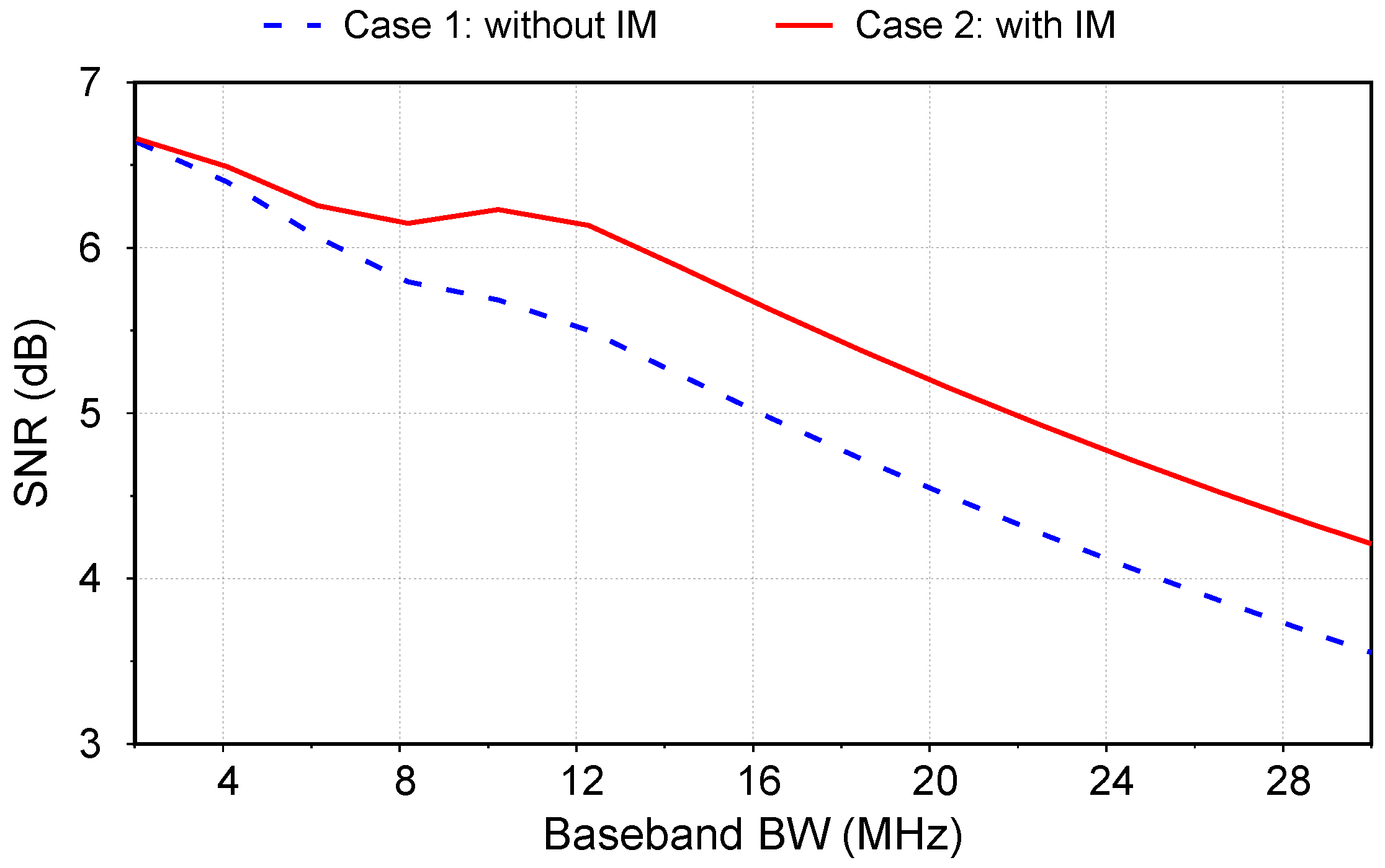
3.2. Signal to Thermal Noise Ratio

The SNR degradation is one of the major issues in iGNSS-R due to the cross correlation of the thermal noise. From [13,16], the final SNR of the power waveform at the output of the cross-correlator is expressed as

$$SNR\left(\tau \right)=\frac{\langle |z_S\left(\tau \right){|}^2\rangle }{\langle |z_{\widehat{S}N}{\left(\tau \right)|}^2\rangle +\langle |z_{S\widehat{N}}{\left(\tau \right)|}^2\rangle +\langle |z_N\left(\tau \right){|}^2\rangle }$$

(3)

where $\langle |z_{\widehat{S}N}\left(\tau \right){|}^2\rangle$ is the average power of cross-correlated up-looking signal and down-looking noise, $\langle |z_{S\widehat{N}}\left(\tau \right){|}^2\rangle$ is the average power of cross-correlated down-looking signal and up-looking noise, and $\langle |z_N\left(\tau \right){|}^2\rangle$ is the average power of cross-correlated up- and down-looking noises.

Using Equations (2) and (3), the SNR of the interferometric power waveform is simulated at the delay corresponding to the specular point (SP), i.e., $\tau =0$, as a function of the receiver baseband bandwidth. As shown in Figure 6, the extra transmitted power of the IM component increases the SNR by $\sim 0.7\mathrm{dB}$ with the bandwidth larger than 10 MHz, which should be taken into account during the design and optimization of iGNSS-R instruments, for example in the link budget calculation and the antenna design. It is worth mentioning that the SNR decreases with the receiver bandwidth, as the thermal noise power is proportional to the latter. The same effect of the receiver bandwidth on the SNR was also reported in [28].

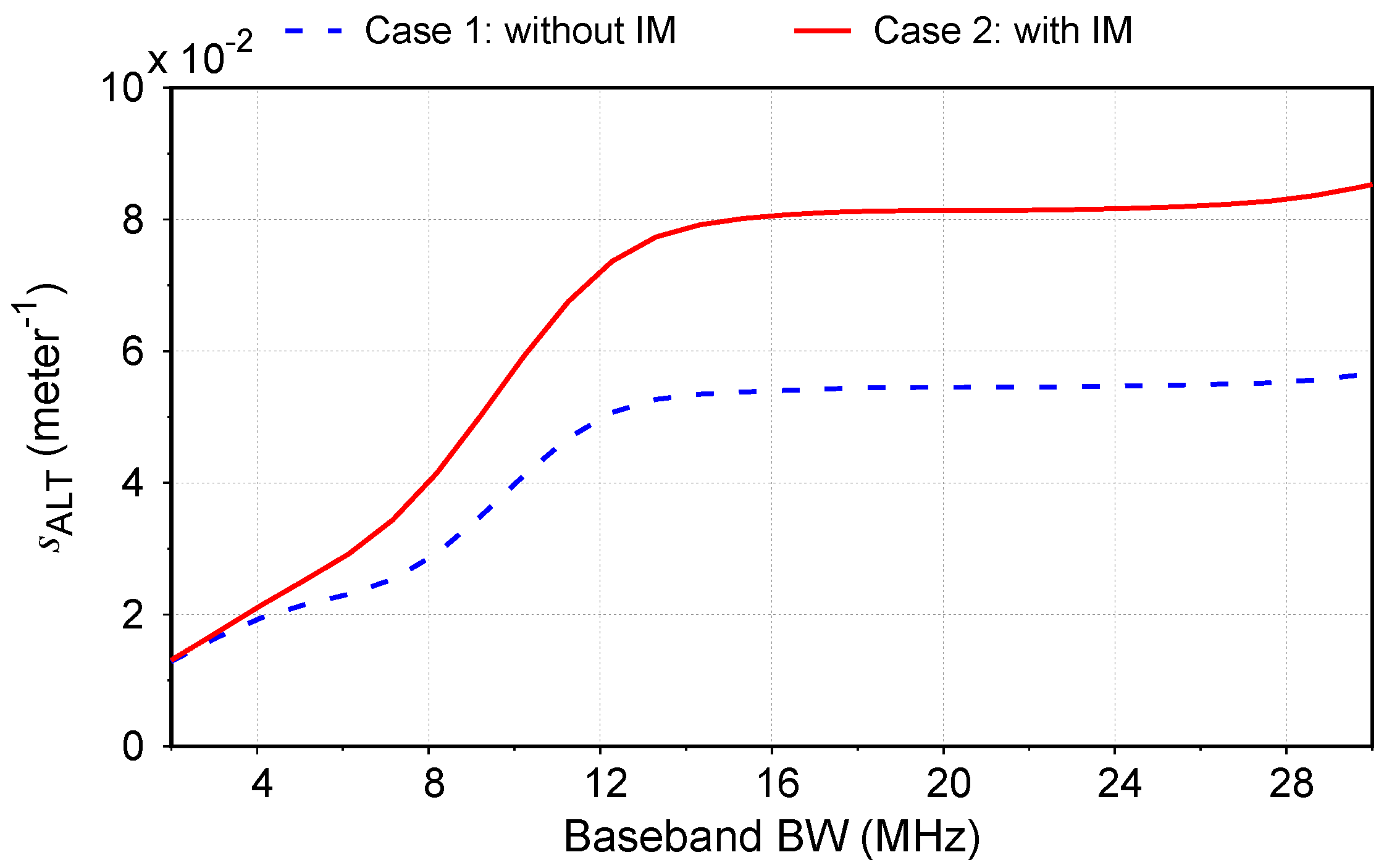
3.3. Altimetric Sensitivity

The leading edge slope of the GNSS-R waveform indicates the altimetric sensitivity of the GNSS signals, which translates the uncertainty of the power measurement to that of the height estimation. By considering the speckle noise, the altimetric sensitivity is defined here as the normalized waveform slope at the delay of the specular point, i.e., $s_{\mathrm{ALT}}={\langle Z_S\left(0\right)\rangle }^{\prime }/\langle c·Z_S\left(0\right)\rangle$, and it mainly depends on the auto-correlation properties of the transmitted signal. As the antenna footprint and the glistening zone are much larger than the pulse limited footprint in a spaceborne scenario, the weight function $W\left(\tau \right)$ in Equation (2) could be approximated as a step function. The slope of the waveform is expressed as

$$\begin{array}{cc}\hfill {\langle Z_S\left(\tau \right)\rangle }^{\prime }& =W^{\prime }\left(\tau \right)\otimes {\mathsf{\Lambda }}_B^2\left(\tau \right)={\mathsf{\Lambda }}_B^2\left(\tau \right)\hfill \\ & ={\left|{\displaystyle {\int }_{-\infty }^{\infty }{S}_C\left(f\right)e^{-j2\pi \tau f}\mathrm{d}f}\right|}^2\hfill \end{array}$$

(4)

in which $S_C\left(f\right)$ is the power spectral density (PSD) of the GNSS signal at the input of the correlator by considering the effects of the front-end and baseband filters. The amplitude of the waveform at the delay of the specular point is expressed as

$$\begin{array}{cc}\hfill \langle Z_S\left(0\right)\rangle & {\displaystyle ={\int }_0^{\infty }{\mathsf{\Lambda }}_B^2\left(\tau \right)d\tau =\frac{1}{2}{\int }_{-\infty }^{\infty }{\mathsf{\Lambda }}_B^2\left(\tau \right)d\tau }\hfill \\ & {\displaystyle =\frac{1}{2}{\int }_{-\infty }^{\infty }{\left|S_C\left(f\right)\right|}^2\mathrm{d}f}\hfill \end{array}$$

(5)

the altimetric sensitivity can be rewritten in the frequency domain

$$s_{\mathrm{ALT}}=\frac{2{\left|{\displaystyle {\int }_{-\infty }^{\infty }{S}_C\left(f\right)\mathrm{d}f}\right|}^2}{{\displaystyle c·{\int }_{-\infty }^{\infty }{\left|S_C\left(f\right)\right|}^2\mathrm{d}f}}$$

(6)

in which c is speed of light in vacuum.

By using the same ideal low-pass filters for both direct and reflected signals, the altimetric sensitivities of the composite signals can be calculated with Equation (6) for two cases with different receiver bandwidths. As shown in Figure 7, including the IM component increases the altimetric sensitivity by a factor of $\sim 1.5$ with the bandwidth larger than 10 MHz, as it concentrates more power further away from the carrier and increases the slope of the power waveform.

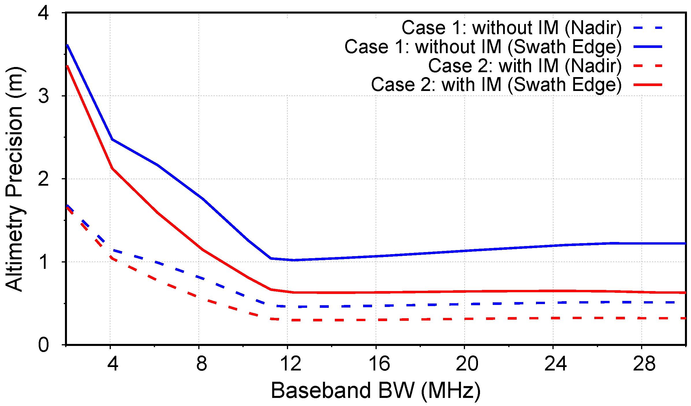
3.4. Precision Analysis

The prediction of the altimetric precision is of primary importance for proper design and optimization of a GNSS-R instrument. In [17,28], comprehensive models were proposed based on the Cramer-Rao Bound (CRB). In this work, a simpler and effective model proposed in [13] is adopted, in which the altimetric precision ${\sigma }_h$ is expressed as a function of the SNR, the altimetric sensitivity, the number of samples incoherently averaged $N_{\mathrm{inc}}$ and the elevation angle ${\theta }_{\mathrm{SP}}$ as

$${\sigma }_h=\frac{1}{2s_{\mathrm{ALT}}sin{\theta }_{\mathrm{SP}}\sqrt{N_{\mathrm{inc}}}}\sqrt{{\left(1+\frac{1}{SNR}\right)}^2+{\left(\frac{1}{SNR}\right)}^2}$$

(7)

Taking the scenario parameters in Table 2 and the instrument parameters from [29], the altimetric precision of the different cases are computed with Equation (7) for different receiver bandwidths as presented in Figure 8. By assuming an optimal receiver baseband bandwidth of 12 MHz, the altimetry precision are summarized in

Table 3. Summary of the altimetric precisions for different cases at nadir and the edge of swath. Case 1: Without IM, Case 2: With IM.

${\mathit{T}}_{\mathbf{inc}}$ (s)	1	5	10
${\sigma }_h$ (m) at Nadir (${\theta }_{\mathrm{SP}}=0^{\circ }$)
Case 1	0.46	0.21	0.15
Case 2	0.30	0.13	0.10
${\sigma }_h$ (m) at Edge of Swath (${\theta }_{\mathrm{SP}}={35}^{\circ }$)
Case 1	1.02	0.46	0.32
Case 2	0.63	0.28	0.19

for different geometries and incoherent average time. These analytical results predict that the altimetric precision is 1.5∼1.7 times better when including the IM component, which should be hence incorporated in the precision budget of iGNSS-R altimetry systems.

4. Conclusions

This research has verified the contribution of the IM component in iGNSS-R waveforms and analysed the impact of this component on GNSS-R interferometric performance for ocean altimetry measurements.

The IM component is a byproduct signal component of CASM in modernized GNSS signals to keep the power envelop of the composite signal constant, which is not officially documented and have been neglected in previous studies on iGNSS-R. This component in GPS L1 band is the product of the ranging components, i.e., the C/A, the P and the M codes, and is equivalent to a BOC(10, 10) signal. The existence of this IM signal increases the total transmitted power and hence the SNR of the iGNSS-R waveform. Moreover, the wide band and split-spectrum properties of this component concentrates more spectral energy farther away from the carrier, and thus improves the altimetric sensitivity. Considering the increase of both the SNR and the altimetric sensitivity, our analysis predicts that the final altimetric precision is 1.5∼1.7 times better when including the IM component. In other words, the altimetric performance of the iGNSS-R has been underestimated in previous studies. This result should be considered for proper design and sizing of the PARIS instrument in future spaceborne GNSS-R altimetry missions, such as the PARIS IoD and GEROS-ISS.

In this work, the GPS L1 band signal is considered as an example of application. It should be noted that the similar IM component also exists in other GNSS signals, which will be transmitting more than two services in each transmission band, such as GPS L2 (with L2C, P and M-code signal), Galileo E1 (with OS Data, OS Pilot and PRS signals), Galileo E6 (with CS Data, CS Pilot and PRS signals), BeiDou B1 (with B1C${}_{\mathrm{D}}$, B1C${}_{\mathrm{P}}$, B1A${}_{\mathrm{D}}$, B1A${}_{\mathrm{P}}$ and B1I signals) and BeiDou B3 (with B3C${}_{\mathrm{D}}$, B3C${}_{\mathrm{P}}$, B3A${}_{\mathrm{D}}$ and B3A${}_{\mathrm{P}}$ signals) [30,31]. The auto-correlation characteristics of these signals should be further studied for the design and optimization of the PARIS altimeter, as well as the altimetric estimator.

References

1. Martín-Neira, M. A passive reflectometry and interferometry system (PARIS): Application to ocean altimetry. ESA J. 1993, 17, 331–355. [Google Scholar]
2. Lowe, S.T.; Zuffada, C.; Chao, Y.; Kroger, P.; Young, L.E.; LaBrecque, J.L. 5-cm-Precision aircraft ocean altimetry using GPS reflections. Geophys. Res. Lett. 2002, 29. [Google Scholar] [CrossRef]
3. Ruffini, G.; Soulat, F.; Caparrini, M.; Germain, O.; Martín-Neira, M. The Eddy Experiment: Accurate GNSS-R ocean altimetry from low altitude aircraft. Geophys. Res. Lett. 2004, 31. [Google Scholar] [CrossRef]
4. Rius, A.; Cardellach, E.; Martin-Neira, M. Altimetric analysis of the sea-surface GPS-reflected signals. IEEE Trans. Geosci. Remote Sens. 2010, 48, 2119–2127. [Google Scholar] [CrossRef]
5. Ghavidel, A.; Camps, A. Time-domain statistics of the electromagnetic bias in GNSS-reflectometry. Remote Sens. 2015, 7, 11151–11162. [Google Scholar] [CrossRef] [Green Version]
6. Carreno-Luengo, H.; Camps, A. Empirical results of a surface-level GNSS-R experiment in a wave channel. Remote Sens. 2015, 7, 7471–7493. [Google Scholar] [CrossRef] [Green Version]
7. Mashburn, J.; Axelrad, P.; Lowe, S.T.; Larson, K.M. An assessment of the precision and accuracy of altimetry retrievals for a Monterey Bay GNSS-R experiment. IEEE J. Sel. Top. Appl. Earth Obs. Remote Sens 2016, 9, 4660–4668. [Google Scholar] [CrossRef]
8. Clarizia, M.P.; Ruf, C.; Cipollini, P.; Zuffada, C. First spaceborne observation of sea surface height using GPS-Reflectometry. Geophys. Res. Lett. 2016, 43, 767–774. [Google Scholar] [CrossRef]
9. Semmling, A.M.; Leister, V.; Saynisch, J.; Zus, F.; Heise, S.; Wickert, J. A phase-altimetric simulator: Studying the sensitivity of earth-reflected GNSS signals to ocean topography. IEEE Trans. Geosci. Remote Sens. 2016, 54, 6791–6802. [Google Scholar] [CrossRef]
10. Zavorotny, V.U.; Gleason, S.; Cardellach, E.; Camps, A. Tutorial on remote sensing using GNSS bistatic radar of opportunity. IEEE Geosci. Remote Sens. Mag. 2014, 2, 8–45. [Google Scholar] [CrossRef]
11. Lowe, S.T.; Meehan, T.; Young, L. Direct signal enhanced semicodeless processing of GNSS surface-reflected signals. IEEE J. Sel. Top. Appl. Earth Obs. Remote Sens. 2014, 7, 1469–1472. [Google Scholar] [CrossRef]
12. Carreno-Luengo, H.; Camps, A.; Ramos-Perez, I.; Rius, A. Experimental evaluation of GNSS-reflectometry altimetric precision using the P (Y) and C/A signals. IEEE J. Sel. Top. Appl. Earth Obs. Remote Sens. 2014, 7, 1493–1500. [Google Scholar] [CrossRef]
13. Martín-Neira, M.; D’Addio, S.; Buck, C.; Floury, N.; Prieto-Cerdeira, R. The PARIS ocean altimeter in-orbit demonstrator. IEEE Trans. Geosci. Remote Sens. 2011, 49, 2209–2237. [Google Scholar] [CrossRef]
14. Wickert, J.; Andersen, O.B.; Beyerle, G.; Cardellach, E.; Chapron, B.; Förste, C.; Gommenginger, C.; Gruber, T.; Hatton, J.; Helm, A.; et al. GEROS-ISS: GNSS reflectometry, radio occultation, and scatterometry onboard the international space station. IEEE J. Sel. Top. Appl. Earth Obs. Remote Sens. 2016, 9, 4552–4581. [Google Scholar] [CrossRef]
15. Cardellach, E.; Rius, A.; Martín-Neira, M.; Fabra, F.; Nogués-Correig, O.; Ribó, S.; Kainulainen, J.; Camps, A.; D’Addio, S. Consolidating the precision of interferometric GNSS-R ocean altimetry using airborne experimental data. IEEE Trans. Geosci. Remote Sens. 2014, 52, 4992–5004. [Google Scholar] [CrossRef]
16. D’Addio, S.; Martín-Neira, M. Comparison of processing techniques for remote sensing of earth-exploiting reflected radio-navigation signals. Electron. Lett. 2013, 49, 292–293. [Google Scholar] [CrossRef]
17. Martín, F.; D’Addio, S.; Camps, A.; Martin-Neira, M. Modeling and analysis of GNSS-R waveforms sample-to-sample correlation. IEEE J. Sel. Top. Appl. Earth Obs. Remote Sens. 2014, 7, 1545–1559. [Google Scholar] [CrossRef]
18. Pascual, D.; Park, H.; Camps, A.; Arroyo, A.A.; Onrubia, R. Simulation and analysis of GNSS-R composite waveforms using GPS and Galileo signals. IEEE J. Sel. Top. Appl. Earth Obs. Remote Sens. 2014, 7, 1461–1468. [Google Scholar] [CrossRef]
19. Martin, F. Interferometric GNSS-R Processing Modeling and Analysis of Advanced Processing Concepts for Altimetry. Ph.D. Thesis, Universitat Politècnica de Catalunya, Barcelona, Spain, 2015. [Google Scholar]
20. Dafesh, P.; Nguyen, T.; Lazar, S. Coherent adaptive subcarrier modulation (CASM) for GPS modernization. In Proceedings of the 1999 National Technical Meeting of The Institute of Navigation, San Diego, CA, USA, 25–27 January 1999; pp. 649–660.
21. Cangiani, G.L. Methods and Apparatus for Multi-Beam, Multi-Signal Transmission For Active Phased Array Antenna. US Patent 6,856,284, 15 February 2005. [Google Scholar]
22. Kukieattikool, P. GNSS Signal Analysis Using High Gain Antenna. Master’s Thesis, Technische Universität München, Munich, Germany, 2009. [Google Scholar]
23. Rebeyrol, E.; Macabiau, C.; Ries, L.; Issler, J.L.; Bousquet, M.; Boucheret, M.L. Interplex Modulation for Navigation Systems at the L1 band. In Proceedings of the 2006 National Technical Meeting of The Institute of Navigation, Monterey, CA, USA, 18–20 January 2006; pp. 100–111.
24. Ribó, S.; Arco-Fernández, J.C. A GNSS-Reflectometry High-Speed Recording Receiver. Remote Sens. 2016, in press. [Google Scholar]
25. Li, W.; Yang, D.; D’Addio, S.; Martin-Neira, M. Partial interferometric processing of reflected GNSS signals for ocean altimetry. IEEE Geosci. Remote Sens. Lett. 2014, 11, 1509–1513. [Google Scholar]
26. Zavorotny, V.U.; Voronovich, A.G. Scattering of GPS signals from the ocean with wind remote sensing application. IEEE Trans. Geosci. Remote Sens. 2000, 38, 951–964. [Google Scholar] [CrossRef]
27. Hajj, G.A.; Zuffada, C. Theoretical description of a bistatic system for ocean altimetry using the GPS signal. Radio Sci. 2003, 38. [Google Scholar] [CrossRef]
28. Pascual, D.; Camps, A.; Martin, F.; Park, H.; Arroyo, A.A.; Onrubia, R. Precision bounds in GNSS-R ocean altimetry. IEEE J. Sel. Top. Appl. Earth Obs. Remote Sens. 2014, 7, 1416–1423. [Google Scholar] [CrossRef]
29. Camps, A.; Park, H.; Domènech, E.V.I.; Pascual, D.; Martin, F.; Rius, A.; Ribo, S.; Benito, J.; Andres-Beivide, A.; Saameno, P.; et al. Optimization and performance analysis of interferometric GNSS-R altimeters: Application to the PARIS IoD mission. IEEE J. Sel. Top. Appl. Earth Obs. Remote Sens. 2014, 7, 1436–1451. [Google Scholar] [CrossRef]
30. Avila-Rodriguez, J.A. Signal Multiplex Techniques for GNSS. Available online: http://www.navipedia.net/index.php/Signal_Multiplex_Techniques_for_GNSS (accessed on 8 December 2016).
31. Xiao, W.; Liu, W.; Sun, G. Modernization milestone: BeiDou M2-S initial signal analysis. GPS Solut. 2016, 20, 125–133. [Google Scholar] [CrossRef]
Figure 1. A simplified block diagram of an interferometric Global Navigation Satellite System Reflectometry (iGNSS-R) receiver.
Remotesensing 08 01013 g001
Figure 2. Comparison between the auto-correlation functions (ACFs) for different signal components in GPS L1 band, i.e., the C/A code, P code, M code and Inter-Modulation (IM) component.
Remotesensing 08 01013 g002
Figure 3. Power spectral density (PSDs) and Woodward Ambiguity Functions (WAFs) of GPS L1 composite signal by considering the IM component. (a) PSDs of the composite signal with and without considering the IM component; (b) Squared ACF of composite GPS L1 signal with and without considering the IM component.
Remotesensing 08 01013 g003
Figure 4. Measured direct waveforms of the GPS L1 in-phase and quadrature components from PRN01. Coherent integration time of T c = 10 ms and incoherent integration time of T inc = 1 s have been used in this example.
Remotesensing 08 01013 g004
Figure 5. Modelled L1 reflected power waveform for the spaceborne scenario in Table 2 with and without considering the IM component. Case 1: GPS L1 without the IM component, Case 2: GPS L1 with the IM component.
Remotesensing 08 01013 g005
Figure 6. SNR as a function of baseband bandwidth considering or not the IM component. Case 1: without IM, Case 2: with IM.
Remotesensing 08 01013 g006
Figure 7. Altimetric sensitivities as a function of baseband bandwidth when considering the IM component. Case 1: without IM, Case 2: with IM.
Remotesensing 08 01013 g007
Figure 8. Altimetric precision at nadir and the edge of swath as a function of baseband bandwidth when considering the IM component. Case 1: without IM, Case 2: with IM. An incoherent average time of 1 s has been used in this example.
Remotesensing 08 01013 g008