Article

Detection of the Coupling between Vegetation Leaf Area and Climate in a Multifunctional Watershed, Northwestern China

1
Key laboratory of Meteorological Disaster, Ministry of Education (KLME)/Joint International Research Laboratory of Climate and Environment Change (ILCEC)/Collaborative Innovation Center on Forecast and Evaluation of Meteorological Disasters (CIC-FEMD)/Jiangsu Key Laboratory of Agricultural Meteorology, Nanjing University of Information Science & Technology, Nanjing 210044, China
2
CAS Key Laboratory of Climate-Environment for East Asia, Institute of Atmospheric Physics, Chinese Academy of Sciences, Beijing 100029, China
3
Center for Forest Disturbance Science, Southern Research Station, United States Department of Agriculture Forest Service, Athens, GA 30602, USA
4
Eastern Forest Environmental Threat Assessment Center, Southern Research Station, United States Department of Agriculture Forest Service, Raleigh, NC 27606, USA
*
Author to whom correspondence should be addressed.
These authors contributed equally to this work.
Remote Sens. 2016, 8(12), 1032; https://doi.org/10.3390/rs8121032
Submission received: 18 September 2016 / Revised: 1 December 2016 / Accepted: 14 December 2016 / Published: 18 December 2016
(This article belongs to the Special Issue Remote Sensing of Land Degradation and Drivers of Change)

Abstract

:
Accurate detection and quantification of vegetation dynamics and drivers of observed climatic and anthropogenic change in space and time is fundamental for our understanding of the atmosphere–biosphere interactions at local and global scales. This case study examined the coupled spatial patterns of vegetation dynamics and climatic variabilities during the past three decades in the Upper Heihe River Basin (UHRB), a complex multiple use watershed in arid northwestern China. We apply empirical orthogonal function (EOF) and singular value decomposition (SVD) analysis to isolate and identify the spatial patterns of satellite-derived leaf area index (LAI) and their close relationship with the variability of an aridity index (AI = Precipitation/Potential Evapotranspiration). Results show that UHRB has become increasingly warm and wet during the past three decades. In general, the rise of air temperature and precipitation had a positive impact on mean LAI at the annual scale. At the monthly scale, LAI variations had a lagged response to climate. Two major coupled spatial change patterns explained 29% and 41% of the LAI dynamics during 1983–2000 and 2001–2010, respectively. The strongest connections between climate and LAI were found in the southwest part of the basin prior to 2000, but they shifted towards the north central area afterwards, suggesting that the sensitivity of LAI to climate varied over time, and that human disturbances might play an important role in altering LAI patterns. At the basin level, the positive effects of regional climate warming and precipitation increase as well as local ecological restoration efforts overwhelmed the negative effects of overgrazing. The study results offer insights about the coupled effects of climatic variability and grazing on ecosystem structure and functions at a watershed scale. Findings from this study are useful for land managers and policy makers to make better decisions in response to climate change in the study region.

Graphical Abstract

1. Introduction

Rebuilding the vegetation covers on degraded lands is an important component of global efforts of restoring ecosystem functions and ecosystem services such as water supply, soil erosion control, carbon sequestration, and biodiversity conservation in many mountain watersheds around the world [1,2]. Accurate detection and quantification of vegetation dynamics and drivers of climatic and anthropogenic change is fundamental for our understanding of the global atmosphere–biosphere interactions [3,4,5,6], and is a prerequisite for the development of strategies for the sustainable management of ecosystems [7]. This is especially critical in dry areas where arid, semi-arid, and dry sub-humid dominate and where climate change and human interactions are believed to have the most impacts on watershed ecosystem functions [1,3].
There is a strong signal showing that northwestern China, a region dominated by an arid and semi-arid climate, has become warmer and wetter since the early 1980s, leading to great changes in vegetation cover in some natural areas [8,9]. This warming and wetting climate has been documented and has stimulated vegetation growth by extending the growing season that promotes plant photosynthesis activities [7,8,10]. The responses of vegetation differ greatly across regions and research scales depending on the kind of changes experienced and the specific response of regional vegetation to those changes [11,12]. However, most of the existing research is performed at a global or large regional level and is seldom done at a basin level [13]. The effective protection of head-water catchments is considered to be an important aspect of the sustainable development of water resources in western China [14,15]. In addition, headwater catchments, which are often forested/naturally vegetated and located in mountainous regions in northwestern China, are areas with high ecological importance such as biodiversity conservation. It is unclear how vegetation responds to climate change in the headwater catchments of arid inland basins where eco-hydrological processes are often complex that involve highly variable precipitation patterns, snow melting, variable evapotranspiration, and permafrost soil hydrology [16,17]. In addition, freshwater resources are experiencing growing resource conflicts between ecosystem demands and economic development due to human population growth and climate change [1,18,19].
The challenges discussed above have been well demonstrated by a large research project at the Heihe River Basin (HRB), China’s second largest inland river basin, which is facing serious ecohydrologial problems in northwestern China. The upper HRB generates nearly 70% of the total river runoff, which supplies irrigation water for agriculture and benefits socio-economic development in the middle and lower HRB [20,21,22]. The vegetation change in the upper reach is a key factor affecting the water balance and catchment water yield. Understanding the complex relationship between spatial vegetation change pattern and climate in this region is important for the integrated inland river basin management. Watershed management of large river systems such as the Heihe River requires close co-operation within the river basin—bringing together all interests upstream and downstream and considering the entire river as one ecosystem and periodically evaluating the ecosystem dynamics over space and time. Therefore, timely monitoring and detecting the response of ecosystems to climate change and other disturbances at a basin level is very important in integrated watershed management to ensure sustainable use of natural resources.
Continuous long-term satellite-based observations provide the only suitable means for consistently characterizing the temporal and spatial dynamics of vegetation across multiple scales. Many previous studies have examined the vegetation response to climate change using satellite-derived Normalized Difference Vegetation Index (NDVI) and ground-based climatic measurements [4,5,23,24,25]. However, vegetation index such as NDVI is easily saturated in the high vegetation coverage areas [26], such as broadleaf forests and needle leaf forests, during the plants’ blooming period. The NDVI did not increase with the growth of vegetation during this period. The NDVI was saturated for 2 months in northwestern China with high-cold meadows and partly cultivated vegetation [27]. Compared with the vegetation index, leaf area index (LAI) is an important vegetation index to represent vegetation conditions on land surfaces. LAI has been widely used to understand the global atmosphere–biosphere interactions and to simulate the land surface processes in Earth System models. In contrast to NDVI, several methods are available for LAI retrieval, being less affected by saturation [28]. However, most of the previous studies on LAI dynamics are limited to short time series vegetation data [23,29] because LAI time series products are less extensive than NDVI products, and long term analysis and the linking of LAI to environmental controls is still relatively rare [4,30].
Linking vegetation change to climate and other disturbances is often challenged by the availability of high resolution meteorological data, especially precipitation data [31]. In addition to the relatively coarse horizontal resolution of atmospheric reanalysis data, it is difficult to reproduce the complex terrain and surface features effectively. Long-term satellite vegetation data combined with downscaled regional climate model data could be applied to compensate for this deficiency.
Various types of mathematical simulation models have been developed to understand environmental controls on vegetation dynamics in recent decades. Dynamic global vegetation model (DGVM) such as CABLE [32], CLM4 [33], ORCHIDEE [34], LPJ [35], VEGAS [36] and MC2 [37] have been created to analyze the broad vegetation response to climate change. However, most DGVMs simulate vegetation changes at a regional or global level, and has been rarely tested at a basin level with such complex terrain and surface features. Simpler statistical methods such as empirical orthogonal function (EOF) and singular value decomposition (SVD) are effective for spatial and temporal analysis [38,39]. Both methods have been used extensively in meteorology and climatology but their applications in regional ecological studies are rare. In this study, we applied EOF and SVD analysis to characterize the spatial patterns of satellite-derived LAI and linked LAI variations to climate variability and human disturbances (i.e., grazing and ecological restoration). The UHRB is a well-studied watershed in ecohydrology in China with a grand goal to couple water resource management and socioeconomics [1]. We took advantage of the rich databases developed for this basin and this work represents a data synthesis effort.
We hypothesized that global warming and increase in precipitation in the UHRB have stimulated vegetation growth which is the dominant factor for the temporal-spatial pattern change of LAI at a basin level. Our overall goal was to synthesize long term remote sensing data and integrate these vegetation data with high resolution climatic modeling data to understand the processes of vegetation change under climatic variation and human pressures. The specific objectives of this case study were: (1) to detect how climate variations in the past three decades (1983–2010) have affected the observed changes in vegetation LAI in a typical inland river basin with very complex topography and landscape; (2) to test the hypothesis that warming and increase in wetness climate variations has stimulated vegetation growth and increased vegetation leaf area, and which is the dominant factor for the temporal-spatial pattern change of LAI; and (3) to explore the implications of multiple driving factors on vegetation change and associated ecosystem function change in a multifunctional land-use watershed in an arid environment. The results contribute to the understanding of regional biophysical and physiological processes under global climate change, and provide critical information to develop methods and strategies towards sustainable development in the study basin and beyond.

2. Materials and Methods
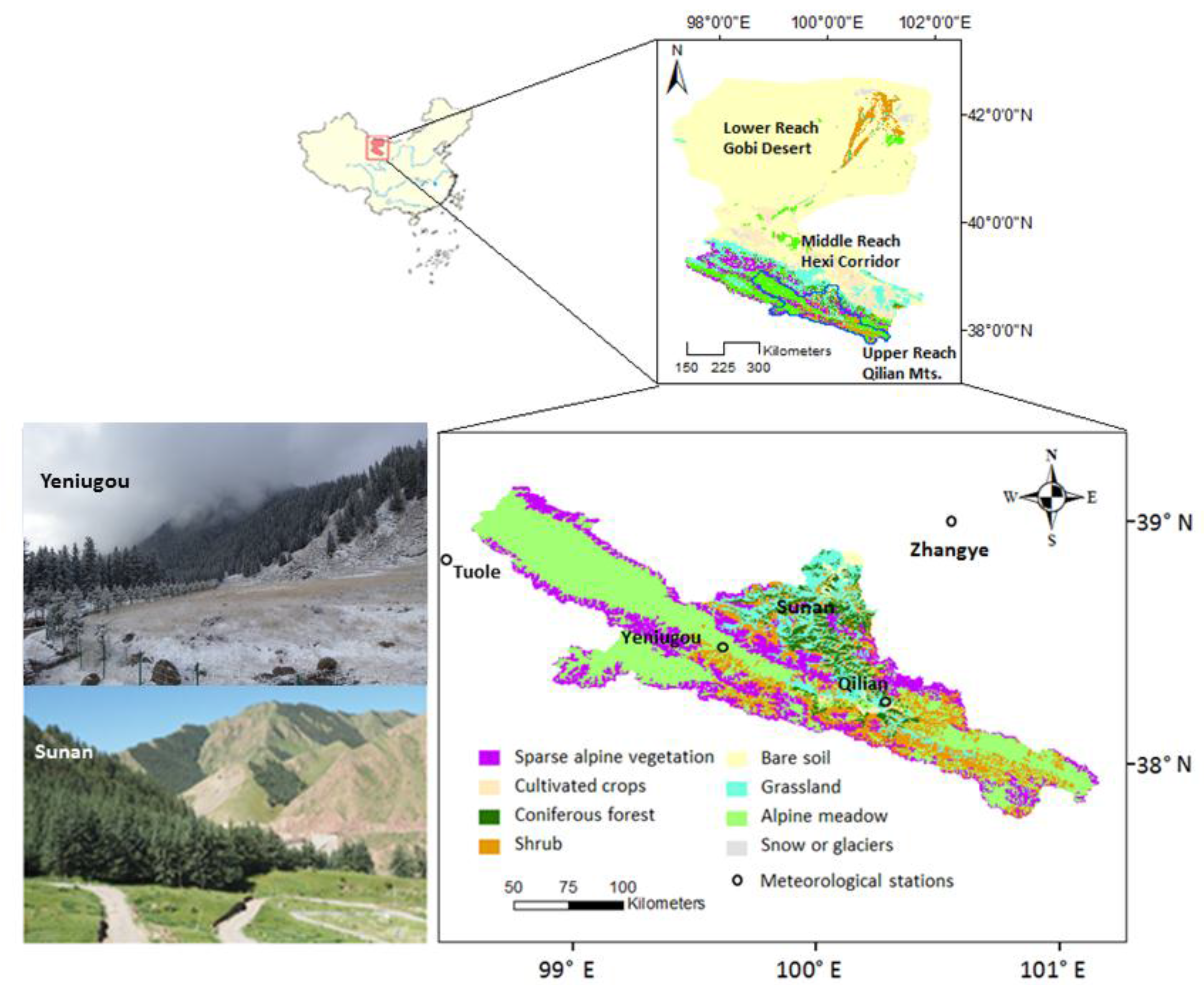
2.1. Study Area

The Heihe River is a typical inland river in arid northwestern China that has received much attention in recent years as a result of rapid ecological degradation, water shortages, and human disturbance. The HRB is divided into the upper, middle and lower reaches, which differ significantly in terms of the natural and socioeconomic characteristics of the three regions. This study focused the upper reach of HRB (UHRB) (Figure 1) (98°34′–101°11′E, 37°41′–39°05′N) that covers an area of approximately 10,005 km2, with an elevation ranging from 1700 m to about 5200 m. The large topographic variations result in relatively abundant vegetation types [22]. The UHRB is administered by Qilian County and Zhangye City extending over the provinces of Qinghai and Gansu, respectively. One of the tributaries, Yeniugou, is located on the southern slope of the Qilian Mountains (Figure 1) with vertical zonality and provides much of the water supply to the Heihe River. The major vegetation types in this basin include coniferous forest, shrub, grassland, alpine meadow and sparse alpine vegetation (Figure 1) [40]. The long-term mean annual precipitation is between 200 mm and 700 mm with a high seasonal variability, and nearly 60% of the total annual precipitation falls in the summer months from June to September. The mean air temperature decreases from about 6.2 °C at low elevations to −9.6 °C at high elevations. In addition to the obvious vertical zonality, horizontal zonality also exists due to precipitation and air temperature gradients from the south to the north and from the east to the west of the basin [41]. Generally, precipitation decreases from the east to the west and increases from the north to the south but the temperature gradient is reversed. In the past three decades, the observed temperature and precipitation show an increasing trend in most areas of the UHRB (Figure S1, Supplementary Material). There are only four meteorological observation stations unevenly distributed around the UHRB (Figure 1) with very complex topographies and landscapes.

2.2. LAI Dataset

In this study, satellite-derived Global Land Surface Satellite (GLASS) LAI datasets were used to assess vegetation growth during the last three decades. The GLASS LAI product (version 3.0) is available from Beijing Normal University (BNU) [42] using an Integerized Sinusoidal (ISIN) projection. The GLASS LAI product is generated from MODIS and AVHRR time-series reflectance data using general regression neural networks (GRNN) [43,44]. The temporal resolution of this dataset is 8 days. From 1982 to 2000, the LAI product is generated from LTDR AVHRR reflectance data with a geographic latitude/longitude projection at a spatial resolution of 0.05° (about 5 km at the Equator). From 2000 to 2012, the GLASS LAI product is derived from MODIS surface-reflectance data with a sinusoidal projection at a spatial resolution of 1 km. Extensive validation on LAI accuracy has been done to make sure the temporally and spatially continuous fields of LAI are reasonable, and the existing results show that the proposed algorithm can obtain a smooth and continuous time series on the LAI during 1982–2012 [44]. The GLASS LAI products derived from MODIS and AVHRR reflectance data represent a consistent data set at a spatial resolution of 0.05°. Comparisons of the GLASS LAI product with the MOD15 and GEOV1 LAI products indicate that these LAI products are generally consistent in their spatial patterns. The global consistency of these LAI products is considered sufficient for ecological studies in most situations, particularly for characterizing grasses/cereal crops and shrubs. Temporal consistency analysis shows that the temporal profiles of all these LAI products are consistent in terms of seasonal variations [45].
The vegetation dynamics were examined for two separate periods: 1983–2000 and 2001–2010, respectively, for the following reasons. First, the resolution of satellite-derived LAI data during the two periods is different (~5 km and 1 km, respectively). Second, the year of 2001 is considered a change point when a series of ecological restoration policies and an ecological protection project in the UHRB were launched and implemented which affect vegetation cover.

2.3. Climate and Aridity Index Data

The monthly or annual meteorological aridity index is defined as AI = P/PET, where P and PET are precipitation and potential evapotranspiration, respectively. This AI is a variant of the dryness index originally defined by Budyko [46]. Previous studies suggest that the radiation-based PET method is more appropriate to quantify PET and water balances as pointed out by Kingston et al. [47], and the PET choice is especially critical for humid, energy-limited regions. However, we do not have access to radiation and wind speed data in this study to apply the Penman-Monteith method for a long-period (1983–2010). We assume that actual water loss in the arid regions is dominated by precipitation and thus the absolute value of PET is not critical to characterizing aridity, so we chose a temperature-based, simpler method to calculate PET. Hamon PET method offers a comparable estimate of potential ET as other more data-demanding methods such as the Penman-Monteith model [48,49]. Therefore, PET was estimated using the Hamon method [50] as a function of saturation vapor pressure (a function of air temperature) weighted by daytime length and inversely proportional to air temperature. The climate was then classified into four types based on AI: arid (AI ≤ 0.2), semi-arid (0.2 < AI ≤ 0.5), sub-humid (0.5 < AI ≤ 1.3), and humid (AI > 1.3) [51] (Figure S2, Supplementary Material).
The climatic data used to calculate AI were created from a regional climate modeling project using the Regional Integrated Environmental Model System (RIEMS 2.0) [31]. The regional simulation was conducted over the period of 1980–2010 with a horizontal spatial resolution of 3 km. The climate model was parameterized with local information, including soil hydrological properties, and recalibrated based on observations and remote sensing data over the HRB. The model evaluation indicated that the model was able to reproduce the spatial pattern and seasonal cycle of precipitation and air temperature. The correlation coefficients between the simulated and observed pentad precipitation were 0.81 in the UHRB regions (p < 0.01) [31]. A high-resolution RCM based on the RIEMS 2.0 [52,53] was used for the HRB. It included the dynamical core of no-hydrostatic version of MM5, the Biosphere-Atmosphere Transfer Scheme (BATS) [54] for surface process representation, cumulus convective parameterization [55,56], and the radiative transfer scheme of the Community Climate Model version 3 (CCM3) [57]. The key parameters of land surface model were recalibrated using the station observational and remote-sensed datasets in the HRB. Various observation datasets were used for model validation. For this study, daily precipitation has been validated against 16 meteorological observation station datasets over the HRB. Global monthly gridded climate data (World-Clim; http://www.worldclim.org) for precipitation averaged over the period 1950–2000 were also evaluated against the RIEMS results [31].

2.4. EOF and SVD Analysis

The empirical orthogonal function (EOF) analysis is widely used to study possible spatial modes (i.e., patterns) of variability and how they change with time. A fundamental advantage of the EOF-based method is to reconstruct the original data by minimizing the noise and the gaps [58]. The singular value decomposition (SVD) analysis is another well-known statistical method [38,39]. SVD is similar to EOF analysis, but, it can be used to detect changes of two variables simultaneously and is capable of identifying spatial patterns of one variable and its relationship to the other one [59,60,61]. The SVD isolates coupled modes of spatial patterns and their associated time expansion coefficients that explain the maximal temporal covariance between two fields.
In this study, we used AI and satellite-derived LAI to conduct the correlation analysis of vegetation and climate. The EOF analysis was first applied to isolate the main patterns of spatial and temporal variability of AI and LAI and to identify significant coherent behaviors of AI and LAI over the watershed. We used monthly and annual SVD to identify the coupling between spatial patterns of LAI and the variability of aridity index (AI) during the two periods of 1983–2000 and 2001–2010, respectively.
In EOF and SVD analysis, the values at every other grid point within the basin were used. The original series of LAI or AI variables at grids were first converted to a monthly/yearly series, which consisted of 216/18 samples for 1983–2000, and 120/10 samples for 2001–2010. The new series was further normalized by subtracting mean from each value and divided by the standard deviation over the samples. The normalized LAI and AI were used for individual analysis by EOF and were paired as left and right fields for SVD analysis. We defined the areas with an absolute minimum value of correlation coefficient passing a 90% confidence level as highly sensitive regions in SVD analysis.

3. Results

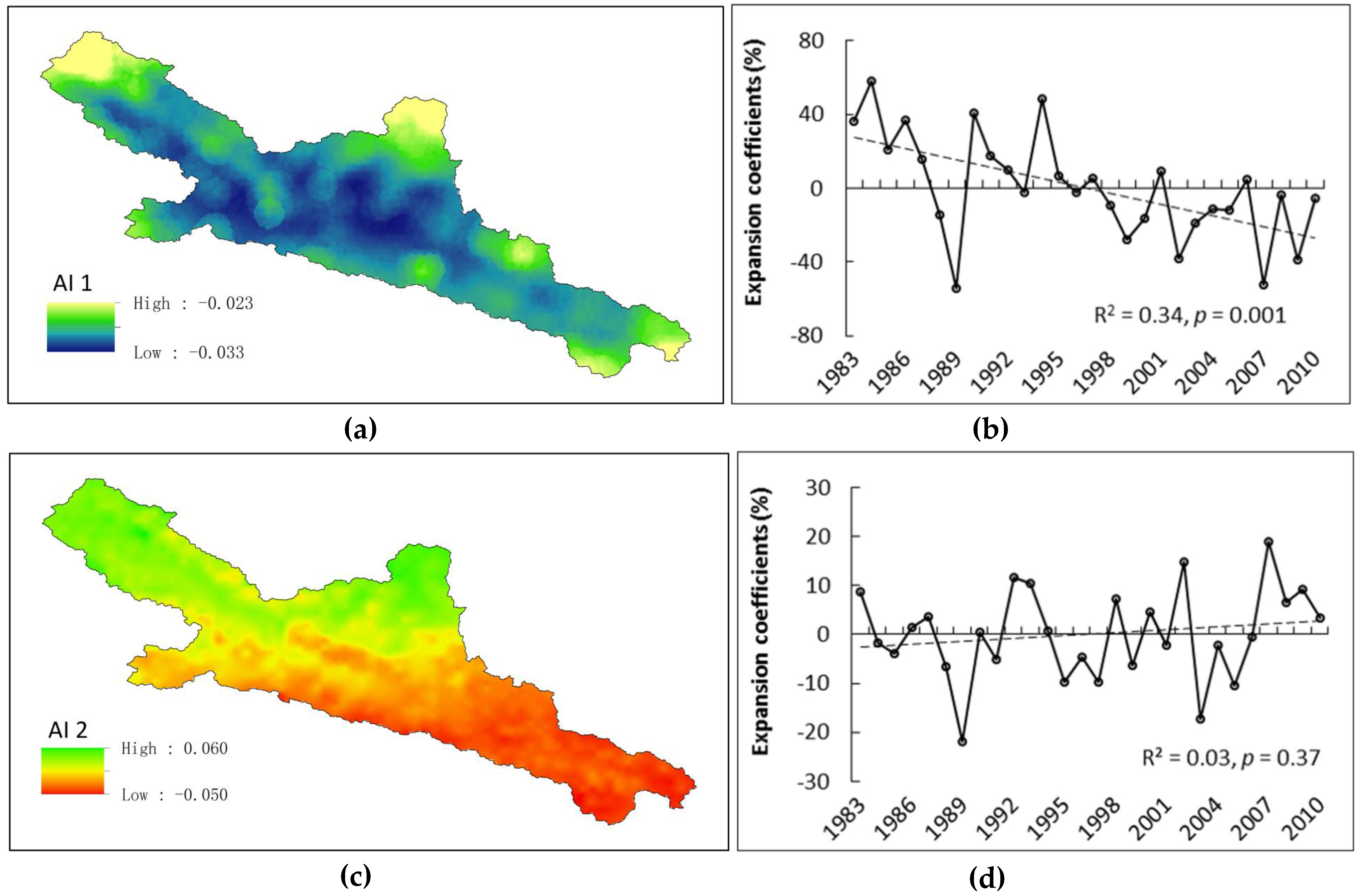
3.1. EOF Patterns of Annual AI

The first pattern of AI accounts for about 77% of the total variance, the second pattern explains only 8.3% (Table 1). Therefore, the first pattern reflects the general dry and humid spatial patterns of the basin. In addition, the first pattern is dominated by one negative anomaly over the entire basin during the period of 1983–2010, which indicates that the whole basin showed consistent dry or humid variation in general during the last 30 years. The maximum negative value region for the first pattern is located in the southwest of the basin (Figure 2a), implying that the AI dynamic in this region is most sensitive and the annual AI trend in the whole basin is dominated by that of the southwest.
The coefficient time series are frequently used to indicate the variance assigned to each EOF. The coefficient time series of the first two EOFs can be found in Figure 2b,d. The values of coefficient time series are proportional to the variance explained by each EOF. The positive values of the first EOF coefficient time series generally indicate drought events, which is also coincident with the drought events observed in this basin, such as in 1986 and 1994. On the contrary, the negative values of the first EOF coefficient time series indicate humid situations. Both the first and second temporal series show a large inter-annual variability, but only the first one shows a linear decreasing trend (Figure 2b), suggesting that the basin is getting wetter, especially in the southwest of the basin. A remarkable feature is the clear change taking place in 1997, showing positive values till 1997 followed by negative values, which indicate that the entire basin becomes wetter after 1997 (Figure 2b). Overall, the first pattern and its decreasing temporal series clearly reveals the drought situation has been eased during the past three decades and the entire basin becomes wetter after 1997.
The spatial distribution of the second pattern exhibits positive and negative anomalies occurring in northwest or southeast pairs (Figure 2c). However, the temporal series of the second mode shows no obvious trend (Figure 2d), indicating that, in addition to the general consistent spatial pattern 1, the UHRB shows regional opposite spatial characteristics. However, these patterns do not show obvious trends.

3.2. EOF Patterns of Annual LAI

The first four EOF and modes represent the major LAI patterns (Table 2). Total LAI change is composed of the first pattern that represents general mean change in LAI and other patterns which reflect regional differences in LAI dynamics.

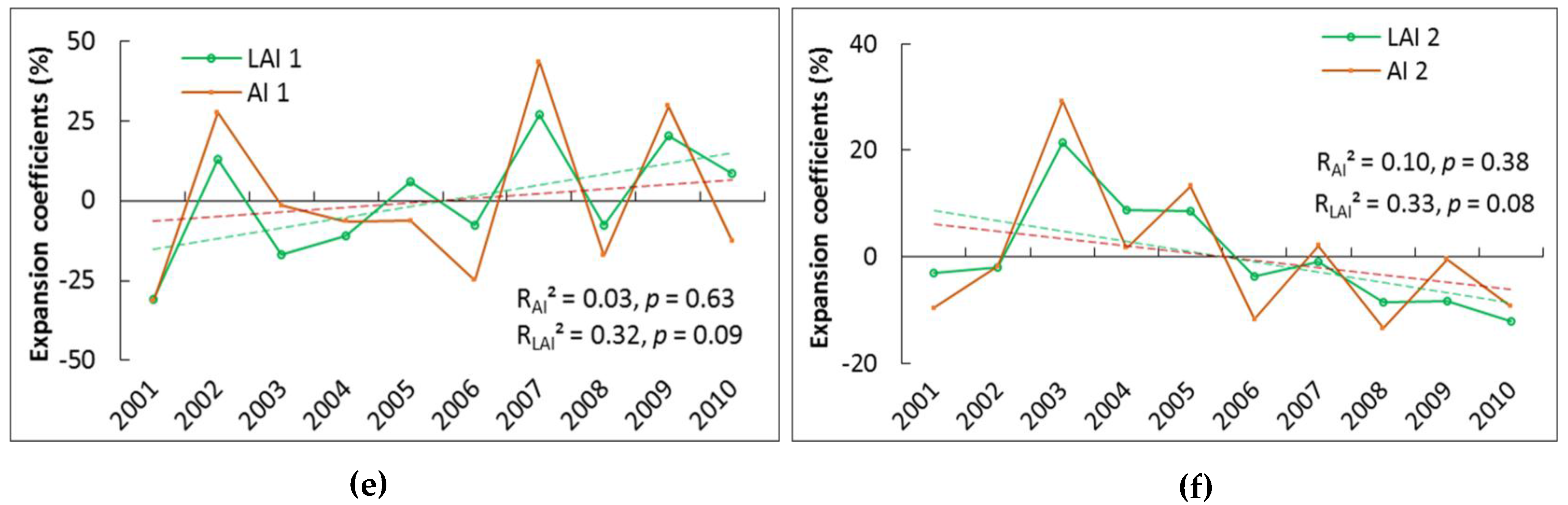
3.2.1. General Spatial Characteristics

During the first period of 1983–2000, the values of the first pattern that represents the general change of LAI over time throughout the basin are almost all negative and account for 26.0% of the total variance and higher than variance explained by any of the other individual patterns (Table 2, Figure 3a). All values in the first pattern (Figure 3a) are negative, which indicate that the vegetation LAI change in this basin has a spatial consistency, i.e., the LAI throughout the entire basin is either improved, or worsened. The maximum negative value region for the first pattern is located in the southwest of the basin (Figure 3a), implying that the LAI dynamics in this region are most sensitive and that the annual vegetation LAI trend in the whole basin is dominated by that pattern in the southwestern part of the basin.
The first pattern during the period of 2001–2010 shows almost all positive values and accounts for 36% of the total variance, which indicates that the vegetation LAI change has a spatial consistency too in the basin level during this period (Figure 4a, Table 2). However, the highly sensitive regions for the first eigenvector shift to the north central part of the basin (Figure 4a).
The negative values of the first LAI EOF coefficient time series generally indicate LAI improved and positive values worsened. Combining the spatial patterns with their temporal series during the period of 1983–2000, we can see that LAI has a similar trend to AI, i.e., both the first and second temporal series show a large inter-annual variability, but only the temporal series of the first pattern shows a linearly decreasing trend (Figure 3b,d), suggesting that the averaged LAI is increasing, especially in the southwest region of the basin. During the period of 1983–2000, however, the averaged LAI values also show an increasing trend, but the highly sensitive area shifts to the north central region of the basin (Figure 4b).

3.2.2. Regional Spatial Characteristics

The second pattern accounts for 15.2% of the total variance for the first period of 1983–2000 and 13.8% for the period of 2001–2010, which accounts for most of the regional difference observed in the LAI change (Table 2). The second pattern for the two periods both show opposite spatial distribution, which indicated that in addition to the general consistent spatial pattern, the UHRB also has regional opposite spatial characteristics (Figure 3c and Figure 4c). The spatial distribution of the third pattern shows a similar opposite pattern with the different increasing and decreasing regions (Figure S3, Supplementary Material). The temporal series of the second (Figure 3d and Figure 4d) and the third pattern (Figure S3, Supplementary Material), show no obvious trend, suggesting that the averaged LAI for these regional patterns has an inter-annual variability and shows no obvious trend.

3.3. SVD Coupling Patterns

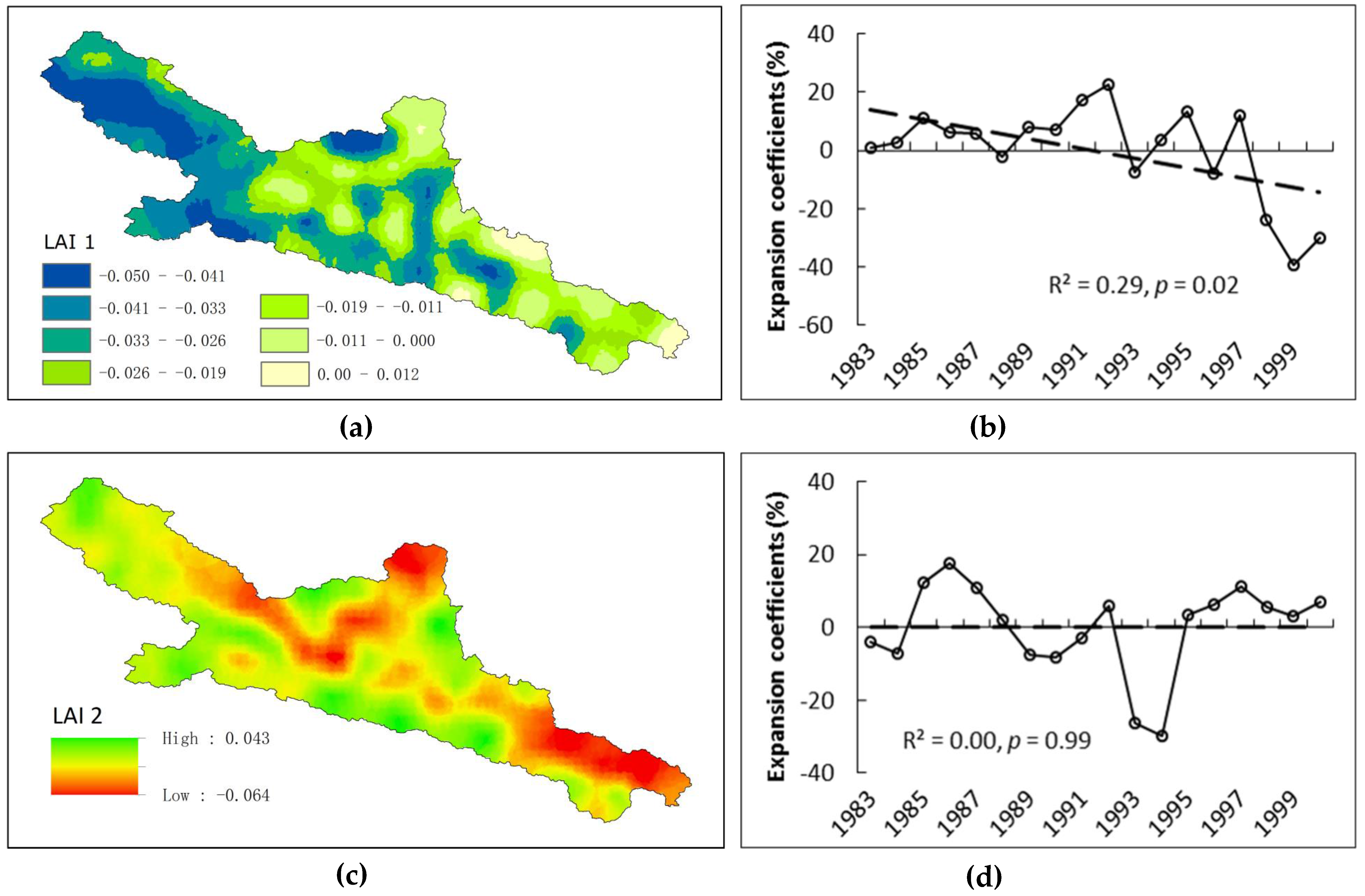
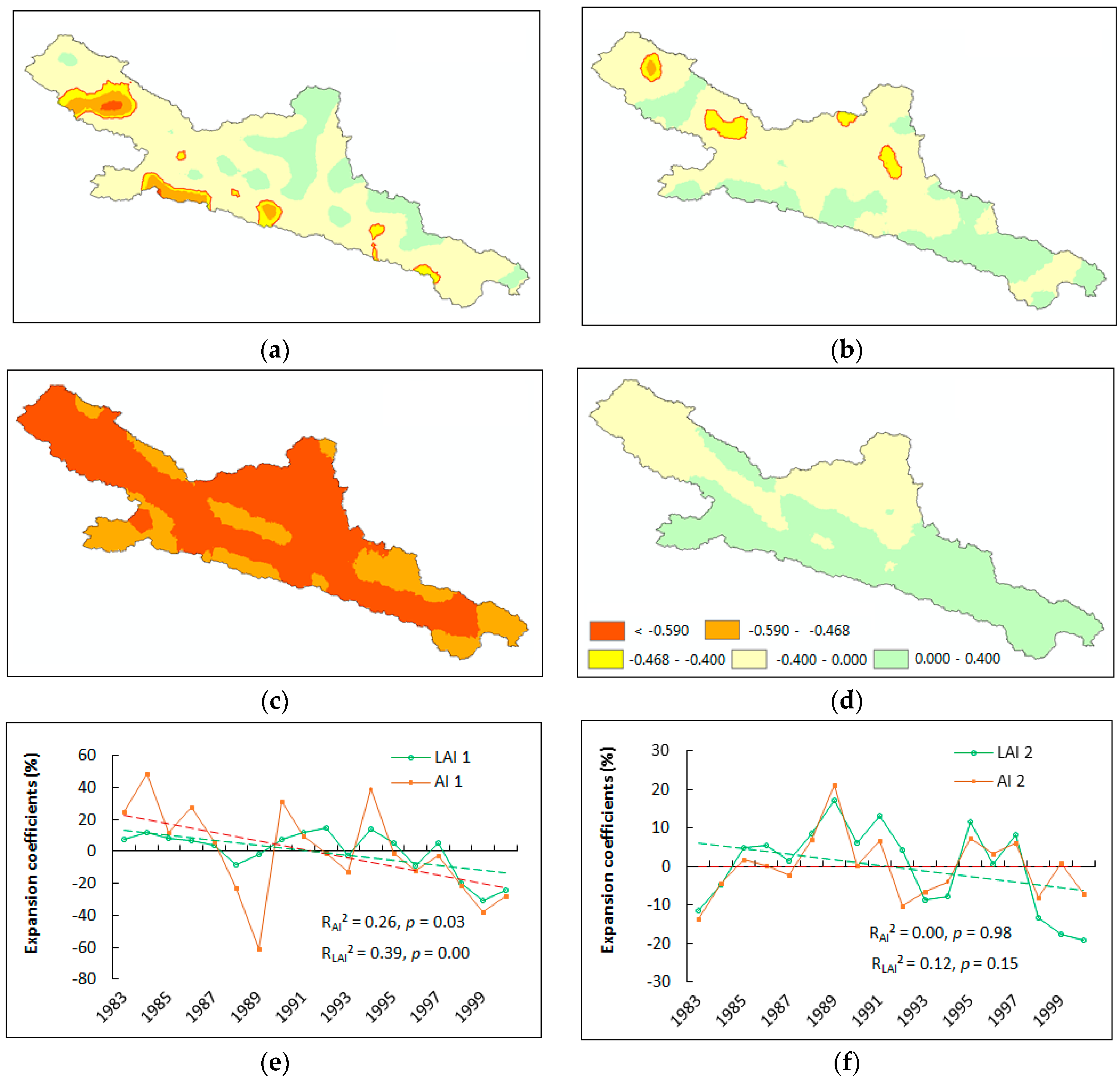
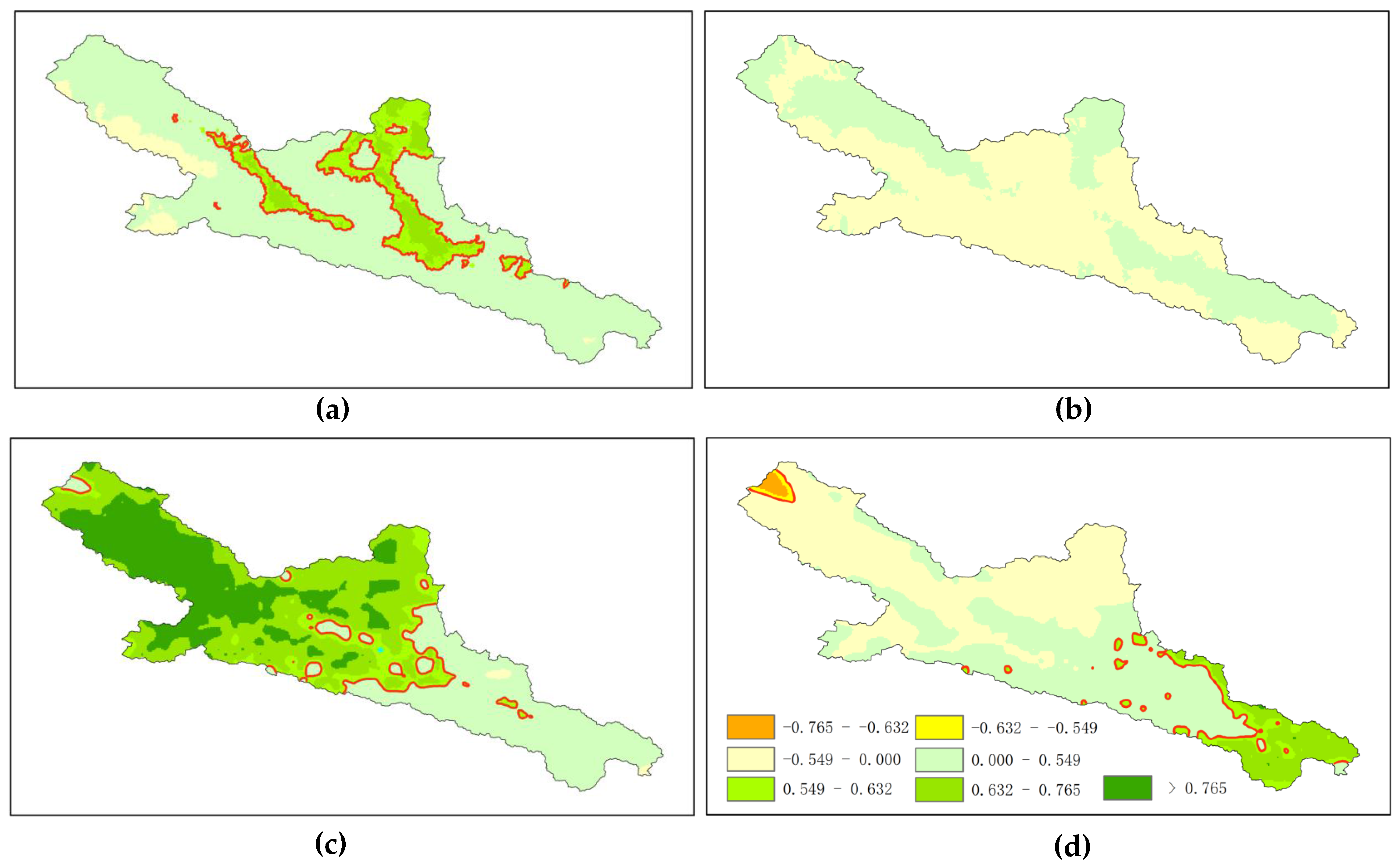
3.3.1. Annual Patterns of 1983–2000

The squared covariance function of the first SVD pattern (SCF1) is greater than 85% (Table 3). The accumulated SCFs (CSCF) are greater than 90% for the first two patterns (CSCF2). The time series ak for LAI and bk for AI are in good agreement with the correlation coefficients rk of 0.72 and 0.74 ( p < 0.001) for the first two patterns. The contributions of the left SVD patterns to the LAI variance, CLAI, are larger for the first mode (17.5%) than the second mode (11.3%). The contributions are about 30% from the first two patterns (Table 3), indicating that about 30% of LAI variance is explained by the first two coupled SVD patterns.
The left heterogeneous correlation coefficient between LAI and AI for the first pattern, denoted here as rleft,LAI,1, reflects the relationship of temporal AI variations with spatial anomalies of LAI, and rright,AI,1 reflects the relationship of temporal LAI variations with AI spatial anomalies for the period of 1983–2000. The rleft,LAI,1 is negative in the southwest basin, and positive in the north and east basin (Figure 5a). The highly sensitive regions of rleft,LAI,1, where the absolute value of the correlation is greater than 0.4 (p < 0.1), are found in the western and southern parts of the basin. The absolute correlation value over 0.47 (p < 0.05) occurs in Yeniugou. The rright,AI,1 is negative across the whole basin (Figure 5c), which means the whole basin is highly sensitive with the absolute maximum values of the correlation coefficient all greater than 0.47 (p < 0.05).
Combining with the temporal series of the expansion coefficients, the analysis suggests that the whole basin is getting wetter (AI is getting larger), LAI decreases in the north and east part of the basin (p > 0.1), increases in the southwestern basin (p > 0.1), and increases significantly in the southwestern part of Yeniugou (p < 0.1) (Figure 5a,c,e).
rleft,LAI,2, the left heterogeneous correlation coefficient between LAI and AI for the second SVD mode, is negative in the north and west and positive in east and south regions (Figure 5b), consistent with rright,AI,2 (Figure 5d).

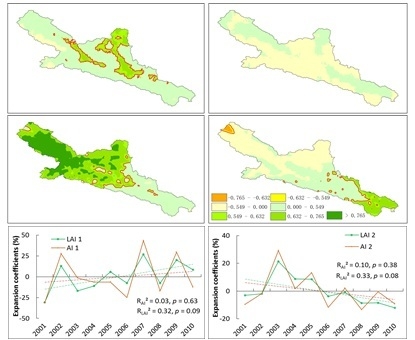
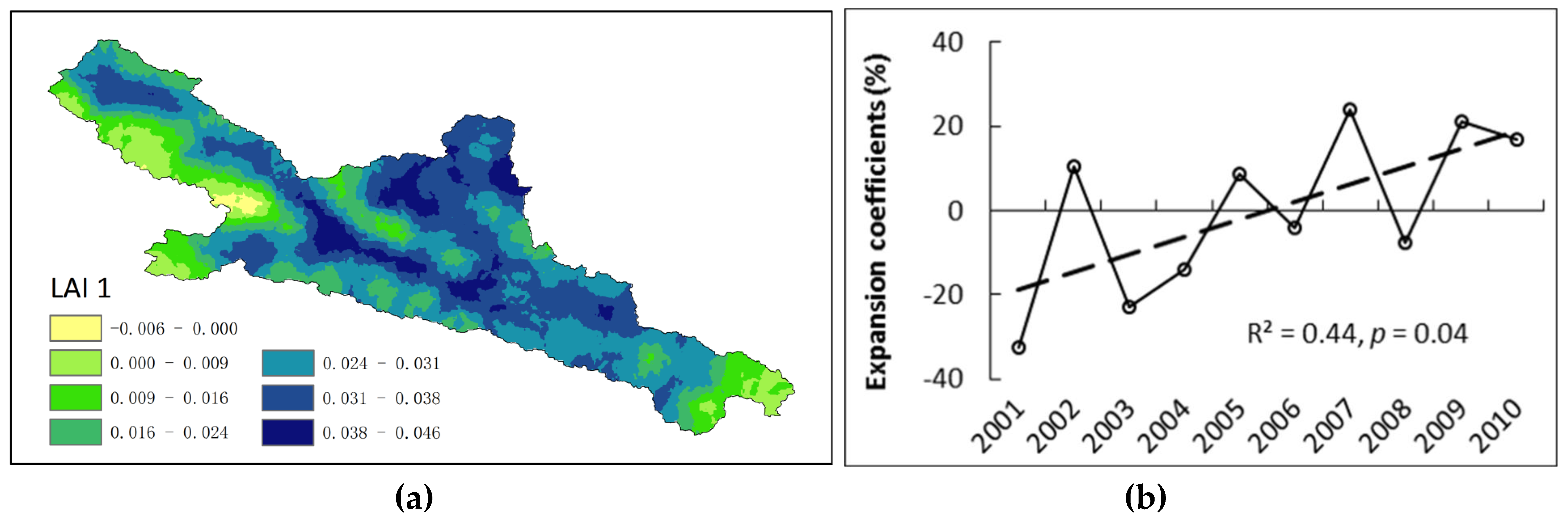
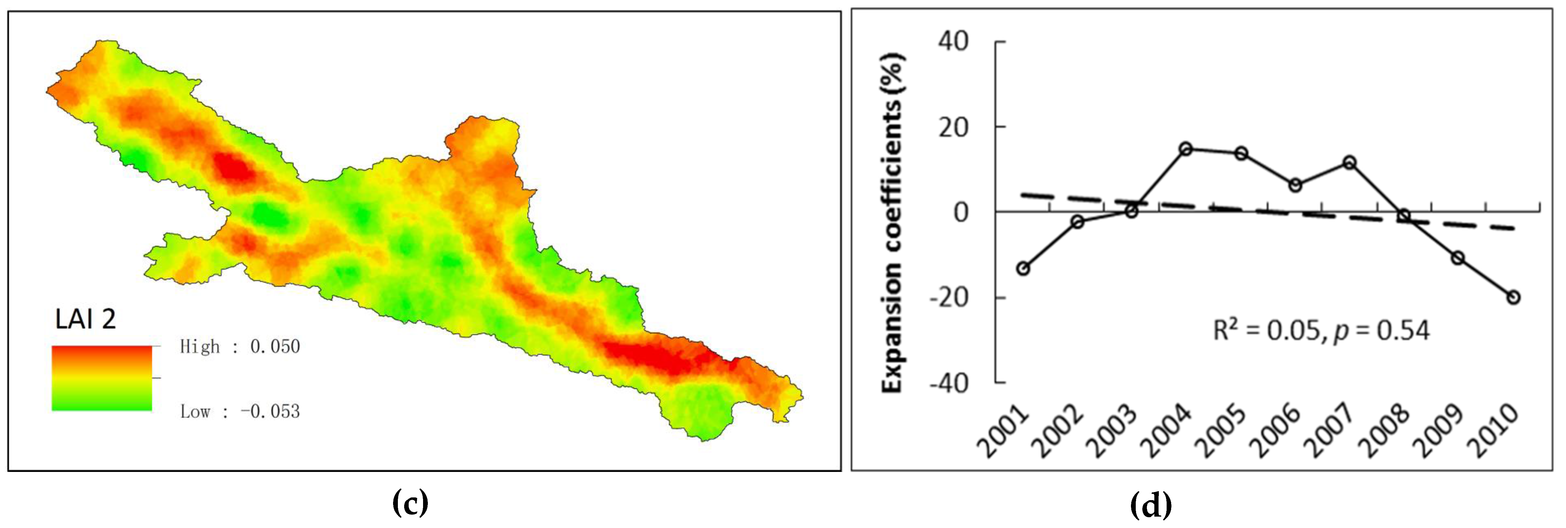
3.3.2. Annual Patterns for the 2001–2010

The squared covariance function of the first SVD mode (SCF1) is greater than 80% (Table 3). The accumulated SCFs (CSCF) is nearly 90% for the first two modes (CSCF2) and 93% for the first three modes (CSCF3). The time series ak for LAI and bk for AI are in good agreement, with the correlation coefficients rk of 0.83 (p < 0.01), 0.89, and 0.94 (p < 0.001) for the first three modes.
The contributions of the left SVD patterns to the LAI variance, CLAI, are much larger for the first mode (31%) than the second mode (10%) (Table 3). The contributions are about 40% from the first two patterns, and about 50% from the first three patterns. This means that about 40% of LAI variance can be explained by the first two coupled SVD patterns and another about 10% by the third patterns.
The left heterogeneous correlation coefficient between LAI and AI for the first pattern, denoted here as Rleft,LAI,1, reflects the relationship of temporal AI variations with LAI spatial anomalies, and Rright,AI,1 reflects the relationship of temporal LAI variations with AI spatial anomalies for the period of 2001–2010.
Different from the first stage, Rleft,LAI,1 and Rright,AI,1 are both positive across most part of the basin (Figure 6a,c). The high sensitive regions of Rleft,LAI,1, where the absolute value of the correlation is greater than 0.55 (p < 0.1), are found in the north central basin, including the northern and central parts of Sunan and the northeastern part of Yeniugou. The highly sensitive regions of Rright,AI,1 are found in the west and central basin, in which Yeniugou is the most sensitive region with a higher absolute correlation of 0.77 (p < 0.01).
Combining with the temporal series (expansion coefficients) (Figure 6e), we can see that as the central and west basin becomes humid (AI is getting larger) (p < 0.1), the vegetation LAI in the north central basin becomes more sensitive to the humid climate and increases significantly (p < 0.1), while most of other regions show an insignificant increase in LAI. As shown before, there is similarity between the SVD patterns of the two fields and their individual EOF patterns.
Rleft,LAI,2, the left heterogeneous correlation coefficient between LAI and AI for the second SVD mode, is negative in the south central basin and positive in the western, eastern and northern parts of the basin (Figure 6b). Combining with the temporal series (Figure 6f), we can see that the LAI decreases with drying in the eastern region, while it decreases in the northern and western regions as DI becomes humid (Figure 6b,d,f).

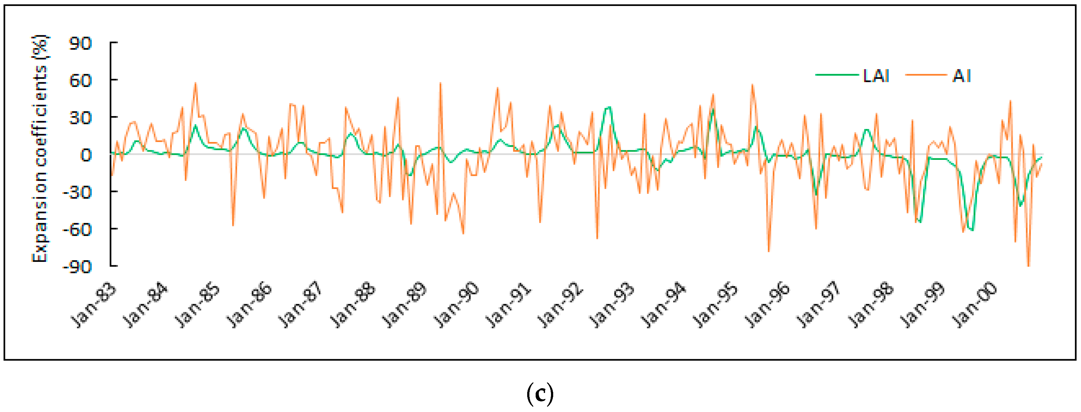
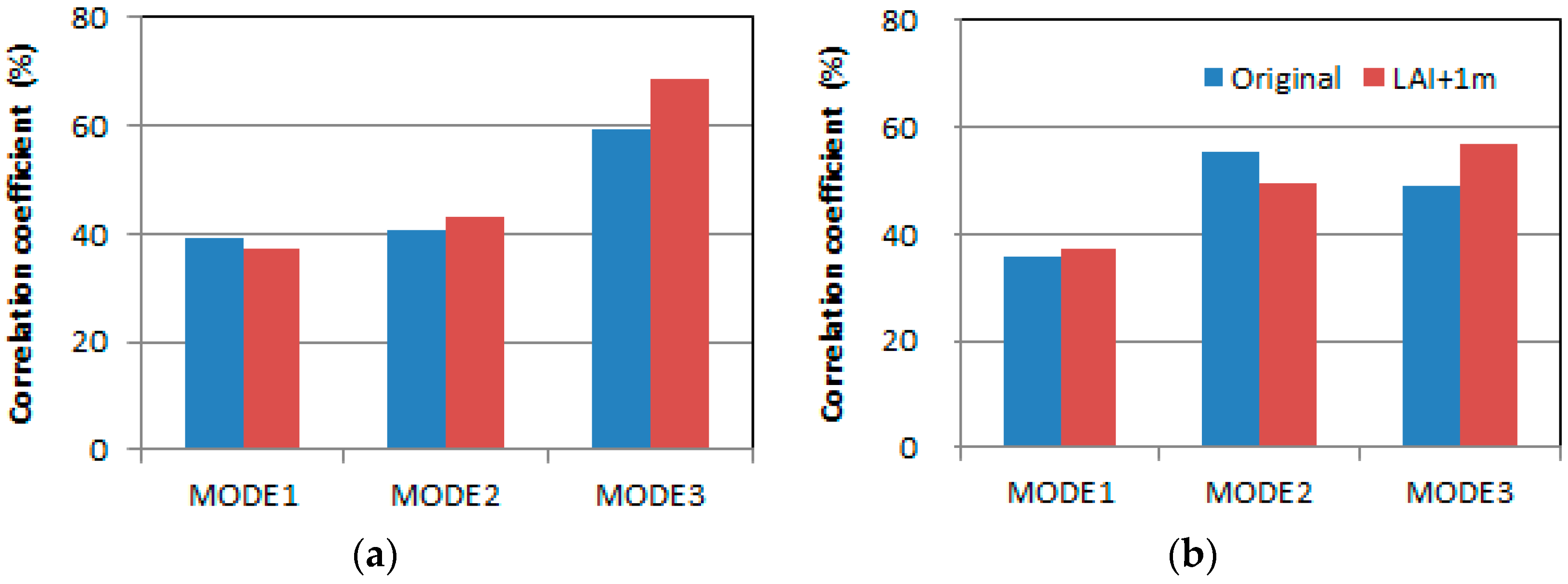
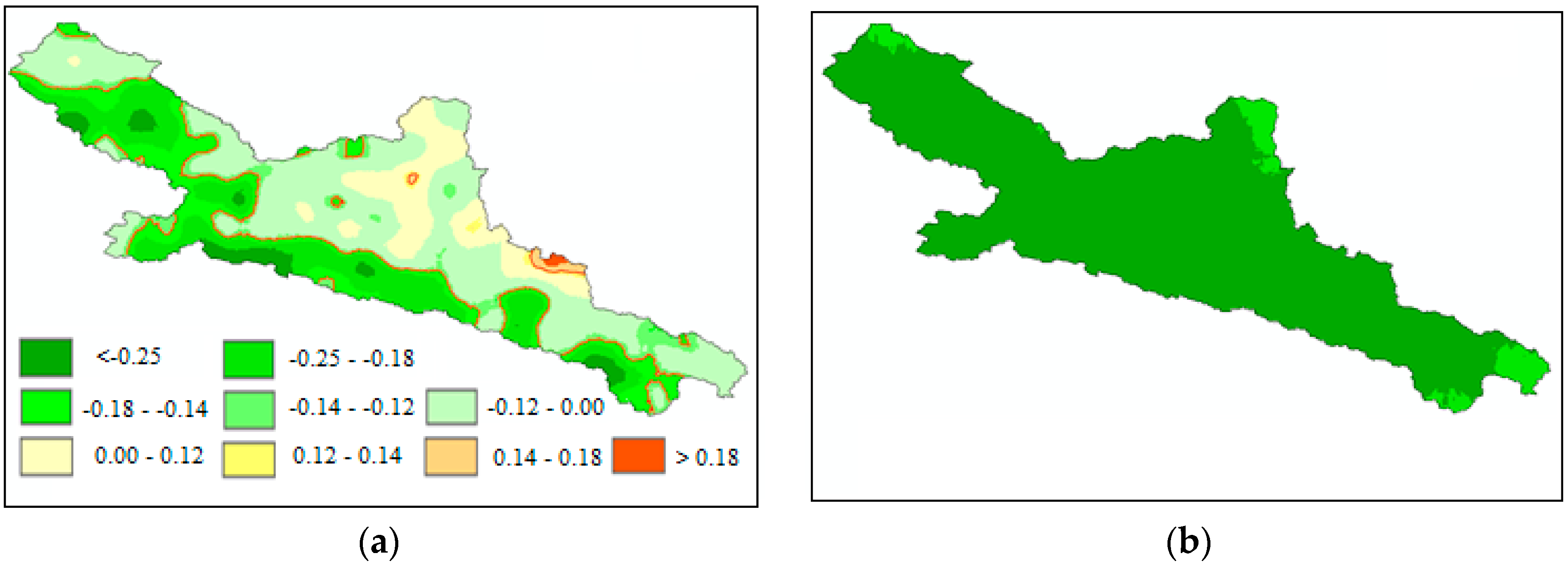
3.3.3. Monthly Patterns

The first monthly SVD mode has a similar pattern to the annual patterns (Figure 7 and Figure 8) but identifies larger sensitive regions in the southwest of the basin during the period of 1983–2000. The correlations for the expansion coefficient series with the first monthly SVD modes are smaller than those with the first annual SVD modes (Table 4), but all pass the 99.9% confidence level. In addition, different from the synchronized change of AI and LAI with the first annual SVD mode, the variations in both frequency and amplitude of AI are greater than that of LAI with the first monthly SVD modes (Figure 7c and Figure 8c).
Comparing both annual and monthly SVD patterns during the two periods of 1983–2000 and 2001–2010, the first two leading SVD patterns depend on AI values and have a cumulative squared covariance of about 90% (Table 3 and Table 4). Therefore, the first two patterns can represent the total variances of annual and monthly LAI anomalies well.
The northeastern and southwestern parts of the basin have opposite annual LAI anomalies in 1983–2000 as indicated by the first leading spatial pattern, but almost identical annual and monthly LAI anomalies across the basin in the late stage of 2001–2010. The most sensitive regions, where the correlations between AI time series and LAI field are statistically significant at the 90% confidence level or higher, are found mainly in the southwestern part of the basin for the first SVD pattern in the early stage, but in the central north of the basin in the late stage (Figure 5, Figure 6, Figure 7 and Figure 8).
The strongest connections occur in the southwestern region before 2000 but afterwards shift to the north central areas with extensive anomalies in the SVD pattern. This suggests that the southwestern region (Yeniugou) and the north central region (Sunan) are the two key regions with high sensitivity of LAI to AI. Before 2000, the highly sensitive region of LAI to the warm and humid climate is located in southwestern region with significant vegetation improvement (p < 0.1). After 2000, however, the vegetation LAI in the north central basin becomes more sensitive to the climate and increases significantly (p < 0.1), while that in the southwestern region shows no obvious increases or even decreases with a significantly warm and humid climate.
During 1983–2000, correlation coefficients with a one month time lag in LAI between monthly SVD expansion series with the second and third SVD mode are 0.43 (p < 0.001) and 0.70 (p < 0.001) respectively, higher than that ignoring the time-lag effects of 0.41 and 0.59 (Figure 9a, Table 4). During 2001–2010, correlation coefficients with the first and third SVD mode are 0.37 (p < 0.001) and 0.57 (p < 0.001) respectively (Figure 9b), also higher than that of the original coefficients of 0.36 and 0.49 (Table 4). However, there is no significant difference between the time-lag correlation coefficients and the original one. This suggests that the LAI is not only determined by climatic factor (AI) within the current month, but also the previous month, i.e., AI could affect the subsequent LAI at monthly scales.

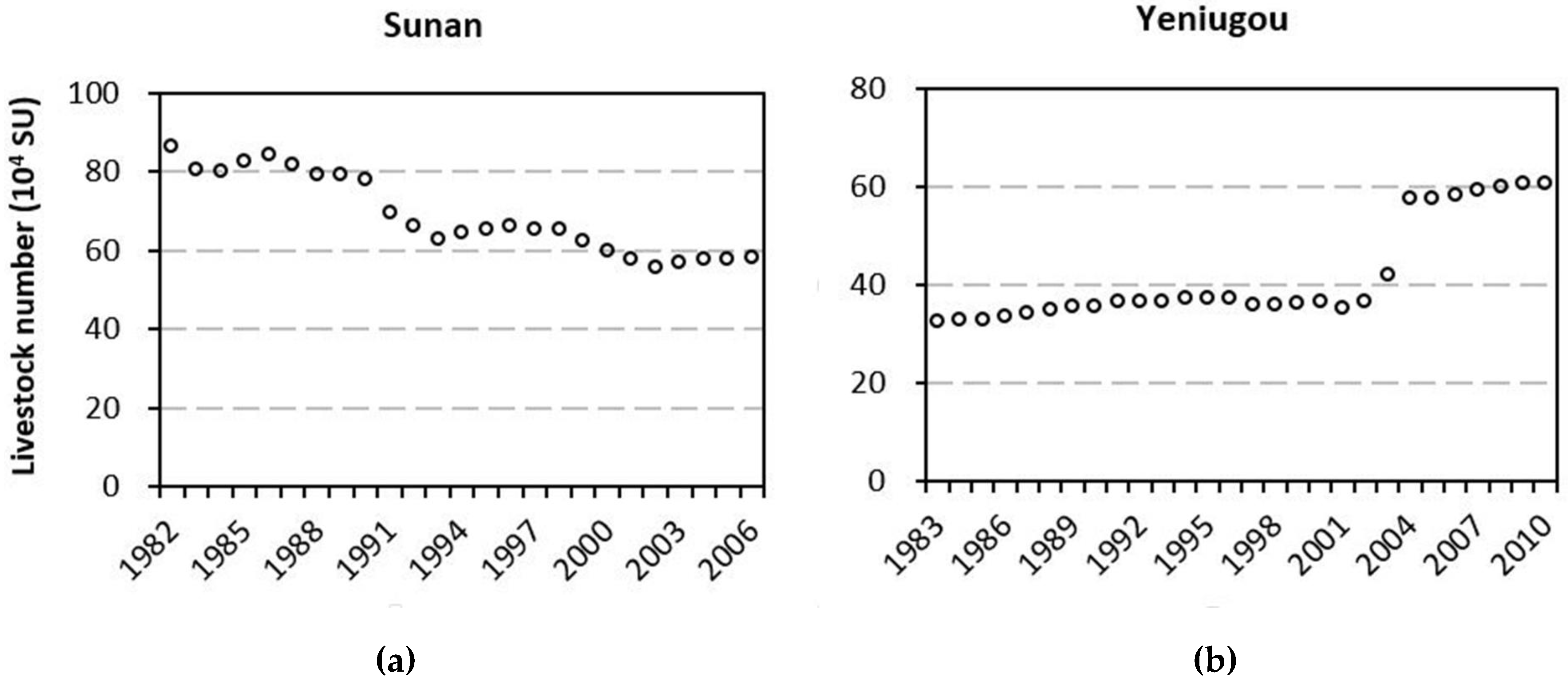
3.4. Grazing History

The livestock numbers in Sunan show a decreasing trend during the past three decades (Figure 10a), while that in Yeniugou shows an increasing trend with a sharp increase in 2004 due to local policy implementation focused on developing animal husbandry (Figure 10b).
The LAI in the growing season has significantly positive correlations with mean minimum temperature and precipitation (R = 0.55, p = 0.01, and R = 0.50, p = 0.025, respectively), but weak negative correlations with overgrazing rate (R = −0.32, p = 0.16) at the basin scale during 1983–2010 (Figure 11).

4. Discussion

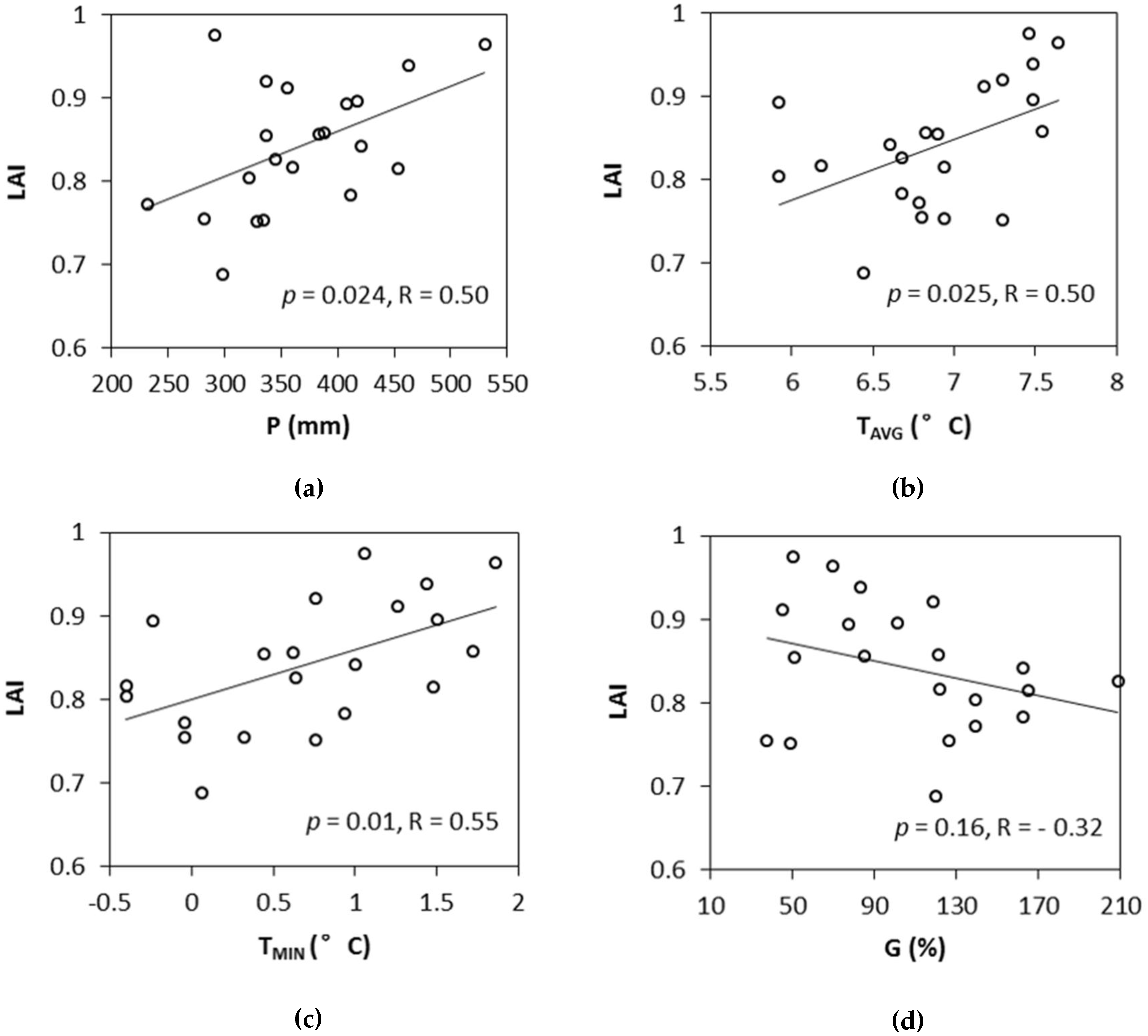
4.1. Effects of AI on the Increase in Vegetation LAI

At regional and continental scales, many studies based on satellite-derived data have established relationships between temporal and spatial changes in vegetation dynamics and climate change and variability [64,65,66,67,68]. For example, the mechanisms for the relationships of vegetation and climate warming in the Qinghai Tibet plateau have been extensively investigated. A warming climate is a major controlling factor for vegetation LAI improvement, especially during the growing season on Qinghai Tibet plateau [4]. Previous studies suggested that this warming has stimulated vegetation growth both through extending the growing season [69,70] and through promoting summer photosynthesis, particularly in energy-limited regions [4,71]. Moreover, the fertilization effects of rising atmospheric CO2 concentration and atmospheric nitrogen (N) deposition have also been considered as possible drivers for greening [4]. The strong connections between AI and LAI with extensive anomalies in the SVD pattern found in our study (Figure 5, Figure 6, Figure 7 and Figure 8, Table 3 and Table 4) supported our hypothesis that a warmer and wetter climate has promoted vegetation growth and increased vegetation leaf area at a basin level. Thus, our study explained the observed increase in LAI. The areas most sensitive to drought-to-humid shifts are mainly located in the sub-humid climate zone, (i.e., northern and western parts of the basin) (Figure S2a, Supplementary Material), especially during the recent decade with significant warming and wetting (Figure 4a,b and Figure 6a,c). This is largely due to the differences in major climate limiting factors (i.e., precipitation or temperature) and the threshold for vegetation growth in the humid and sub-humid climatic zones, respectively [69].
The time-lag effects found in this study are important for better predicting and evaluating the vegetation dynamics under global climate change [72]. Wu et al. [72] found that the time lag of NDVI to precipitation in arid and semi-arid areas is approximately 1 month, but does not exhibit time-lag effects to temperature. Research in Kansas, USA, also demonstrated that the time-lag of grassland ecosystems to precipitation was 1 month [73]. Our findings are partially consistent with previous studies. The results show that the vegetation LAI exhibits a 1 month time-lag effect to AI, but no time-lag effects to AI at annual scale, which indicates that the LAI in the UHRB is not only determined by climatic factor (AI) within the current month, but also the previous month. The climatic influence on the vegetation LAI has a scale-effect, and the response of LAI to AI is diverse at different time scales.

4.2. Potential Extreme Climate Effect on LAI

A key feature of current climate change is the increasing frequency of extreme climate events, particularly droughts [74]. Evidence exists that extreme climate events impact a broad range of ecosystems [75,76,77]. Moreover, according to IPCC climate models, it is likely that such extreme events will become more frequent and more intense in the future, although there is considerable uncertainty in climate model predictions [64]. The increase in temperatures on the Qinghai Tibet plateau has been much greater than other regions of the world in recent decades [78,79], and there may be a trend with more warming in the future, but uncertainty in precipitation [10,80]. Recent observational and experimental studies have highlighted the potential for warmer temperatures to compound the effects of severe drought events and exacerbate regional vegetation stress [81,82,83].
During the past three decades, although the warming and improved water conditions, as well as ecological restoration policies in the UHRB have caused a significant increase in vegetation LAI, regional grassland degradation due to intensive overgrazing is still very common. The potential increasing frequency of extreme climate events, particularly droughts, could aggravate the negative effect of overgrazing on the vegetation. Therefore, understanding the consequences of the increased incidence of extreme climatic events on ecosystems is emerging as one of the grand challenges for global change scientists [75,84].

4.3. Other Factors Affecting LAI

Our results show that the vegetation in the southwestern part (Yeniugou) of the basin was significantly improved with the increasing air temperature and precipitation prior to the year 2000, but there was no significant improvement afterwards under similar climate conditions. On the contrary, after 2000, there was a decline in LAI in the southern part of Yeniugou, the source of the Heihe River (Figure 5, Figure 6, Figure 7 and Figure 8). This complex spatial and temporal pattern indicates that the driving factors of LAI are spatially variable. The role of the increases in AI for stimulating LAI might have masked the potential decreases due to grazing in the overall spatially averaged LAI at the basin scale due to other factors. In recent decades, although a series of ecological restoration policies and ecological protection projects have been implemented in this region, intensive overgrazing (Figure 10 and Figure 11), as well as gold mining, herb-medicine harvesting, and damages caused by plateau pikas (Ochotona curzoniae) [85,86] have been intensified contributing to vegetation deterioration [62]. In addition, the significant increase in temperature also resulted in accelerated permafrost thawing and glacier retreat [87], which might have caused and exacerbated the degradation of alpine grassland [88] and wetlands [89].
On the other hand, the vegetation LAI values show decreases in the north central region (Sunan) as the whole basin is getting wetter in the early stage, but becoming more sensitive to the increasingly wetter climate in the late period (Figure 5, Figure 6, Figure 7 and Figure 8), suggesting a significant improvement in vegetation. Sunan is one of the important grazing counties in Zhangye City. Overgrazing leads to severe grassland deterioration in this region [90] (Figure 10a). Since 2000, the Chinese government is investing 2.35 billion RMB to implement ecological restoration policies in Heihe River basin. Previous studies have concluded that human activities such as afforestation and grazing exclusion management can potentially contribute to the satellite-observed greening of China’s vegetation over the last three decades [4,62,63,91,92]. Therefore, grazing exclusion and afforestation may contribute to the significant improvement in local vegetation cover in the late stage.

4.4. Regional Implications

Previous comprehensive regional studies [7,23,25,69] report a general greening trend in northwestern China and have attributed the trend to the positive effects of a warming climate. However, the vegetation responses to climate differ across regions depending on many kinds of changes experienced and the specific response of regional vegetation to those changes including both climate and human activities. For example, land management practices such as grazing may mask climate effects while periodic droughts may mask the positive effects of ecological restoration in some areas. The present watershed-level study advances our understanding of the processes of climatic and human disturbances to vegetation. The research method using long term satellite-derived leaf area index (LAI) datasets and downscaling regional climate gridded data series is well equipped to study long term patterns.
Study results have important environmental implications for mountainous basins in China and elsewhere with a similar environment such as the Eurasia highlands [3]. Our findings provide additional information on the effectiveness of the recent massive afforestation and ecological restoration campaigns in this region. The study results can also provide data to improve process-based dynamic vegetation models. Further analysis identifying and quantifying the contributions of each factor by applying optimized regional dynamic vegetation models, structural equation models or other methods may be valuable for improving our understanding of the roles of multi-impact factors in LAI.

4.5. Uncertainties

The GLASS LAI dataset is based on different sensors: AVHRR from 1982 to 1999 and MODIS from 2000 to 2013. So, the consistency of the two dataset and their validation are very important. Xiao et al. [45] recently examined the consistency between the GLASS LAI products derived from AVHRR and those from MODIS data for the period of 1982–2012. According to Xiao et al., to assess spatial and temporal consistencies between the LAI values, both datasets were re-projected and were aggregated to a resolution of 0.05° using a spatial-average method [45]. LAI profiles from 1982 to 2012 over several sites with different land-cover types were analyzed to check the temporal consistency of the GLASS LAI values derived from MODIS and AVHRR reflectance data. Direct validation with the mean values of high resolution LAI maps demonstrates that the GLASS LAI values were closer to the mean values of the high-resolution LAI maps (the root mean square error RMSE = 0.79, the coefficient of determination R2 = 0.81) than the GEOV1 LAI values (RMSE = 0.91, R2 = 0.79) and the MOD15 LAI values (RMSE = 1.12, R2 = 0.67) [45]. The validation of LAI products with ground measurements, however, was limited. Most ground-based validation has been conducted since 2000 [93]. Liang et al. [94] also indicated that the GLASS product is of higher quality and accuracy than the existing products, and in particular, it has much longer time series, and is therefore highly suitable for various environmental studies.
On the other hand, the SVD analysis method can effectively reduce the error of the LAI data in this study. The SVD method has the ability to identify the most relevant parts of the two from the changes in LAI and AI. Although GLASS LAI data contains errors, these errors are not necessarily linked to the inter-annual variation in climate. It can be proved that if random errors were added artificially to the LAI data, the final analysis results will not be significantly different [95]. Therefore, it is concluded that the influence of LAI error on the analysis results of this paper should be very small, which does not affect the conclusion of this study.
Generally, for most temporal and spatial analysis methods such as EOF, the accuracies often depend on the amount of spatial samples. Studies using data sets with different sample sizes often have different conclusions. In this study, we used both EOF and SVD for temporal and spatial analysis. As shown before, there is a similarity between the SVD patterns of the two fields and their individual EOF patterns. In addition, comparing SVD patterns at both annual and monthly scales, the leading SVD modes have similar patterns (Figure 5, Figure 6, Figure 7 and Figure 8) and a cumulative squared covariance of about 90% (Table 3 and Table 4). This indicates that the results obtained by SVD are stable. The strong correlation between LAI and AI does not change with variations in spatial sample size.
A reliable simulation of the land-atmospheric processes is essential to understanding the importance of spatial patterns of vegetation connected to the climate. As in other climate models, precipitation data from the regional climate model adopted have great uncertainties, which certainly would affect our assessment results. In this study, the simulated precipitation in the UHRB was closer to the observational data because key parameters within the land surface process that affect the energy and water balance were recalibrated [31]. At the same time, it should be pointed out that bias of precipitation in the UHRB is larger than that in other regions of the HRB. Continuous efforts in developing parameterizations of precipitation are critical to enhancing our understanding of atmospheric and vegetation processes.

5. Conclusions

This work offers an effective integrated approach to detect the coupled spatial patterns of vegetation dynamics and climate variations during the past three decades in a multifunctional land-use watershed. Long-term remote sensing derived LAI data, downscaled climatic data created from a regional climate modeling, and advanced statistical methods (EOF, SVD analysis) were adapted in this study. The continuous long-term Earth Observation (EO) satellite data provide temporally and spatially consistent data analysis across multiple scales [6], as well as an effective way to combine it with SVD analysis and regional climate models for the assessment and monitoring of environmental changes in multifunctional land-use watersheds with very complex topography and landscapes.
The spatial and temporal variations of LAI patterns of the study basin are explained by the coupling patterns of LAI and the variability of the aridity index (AI). During the past three decades, the study area has become wetter resulting in an increase in LAI as a whole. Climate (AI) could affect LAI at a monthly scale with a time lag, suggesting that climatic influence on vegetation LAI has a scale-effect.
We also found that the spatial change patterns of LAI in a watershed shifted over time. These complex spatial and temporal patterns indicate that the driving factors of LAI are very complex in this basin. Climate change and variability (i.e., increase in AI) appear to be primarily responsible for the LAI improvement throughout the basin, and the effect of drought-to-humid shifts on LAI mainly depends on climate zones. Human disturbances such as ecological restoration policies and intensive overgrazing may differ among the various sub-regions and also contribute to local LAI variations. Overall, at the basin level, the general positive effects of climate warming and precipitation as well as local ecological restoration efforts overwhelmed the negative effects of overgrazing. In a particular climate zone, human activities can magnify or reduce the risk of present and future drought on vegetation in the context of global warming.
Minimizing and mitigating the negative impacts from climate change and human disturbances and maintaining ecosystem sustainability requires an integrated watershed management approach that involves careful basin planning [1,3], landscape design [96], and grazing management [83,97]. Future studies should focus on understanding the biophysical processes that affect LAI of ecosystems in a complex terrain. Methods (EOF and SVD) developed from this case study should be tested in a similar region to further improve their applicability.

Supplementary Materials

The following are available online at www.mdpi.com/2072-4292/8/12/1032/s1, Figure S1: Air temperature anomaly (°C, red lines) and precipitation anomaly percentage (%, grey bars) in four meteorological stations (a) Tuole; (b) Yeniugou; (c) Zhangye; and (d) Qilian (Figure 1 showed the locations of the four stations); Figure S2: Mean annual AI during (a) 1983–2000; and (b) 2001–2010; and Figure S3: EOF of annual LAI (a) Mode 3; (b) Temporal series of Mode 3 during 1983–2000; (c) Mode 3; and (d) Temporal series of Mode 3 during 2001–2010.

Acknowledgments

This research was funded by the Natural Science Foundation of China (Grant No. 91425301, 41571026 and 71373130). We thank the three anonymous reviewers and associate editor for their constructive comments and suggestions. We thank the China Meteorological Administration, Beijing Normal University, and Cold and Arid Regions Science Data Center for sharing the climate and vegetation data. Partial support was also received from the Southern Research Station, United States Department of Agriculture Forest Service.

Author Contributions

Lu Hao conceived and designed the research; Lu Hao, Cen Pan and Peilong Liu performed the research; Cen Pan, Peilong Liu and Liangxia Zhang analyzed the data; Zhe Xiong created the climate dataset; Cen Pan and Lu Hao wrote the paper; Ge Sun, Yongqiang Liu and Decheng Zhou supervised the research, and reviewed the paper.

Conflicts of Interest

The authors declare no conflict of interest.

References

  1. Li, X.; Cheng, G.; Liu, S.; Xiao, Q.; Ma, M.; Jin, R.; Che, T.; Liu, Q.; Wang, W.; Qi, Y. Heihe watershed allied telemetry experimental research (HiWATER): Scientific objectives and experimental design. Bull. Am. Meteorol. Soc. 2013, 94, 1145–1160. [Google Scholar] [CrossRef]
  2. Sun, G.; Feng, X.; Xiao, J.; Shiklomanov, A.; Wang, S.; Zhang, Z.; Lu, N.; Wang, S.; Chen, L.; Fu, B.; et al. Impacts of global change on water resources in dryland East Asia. In Dryland East Asia: Land Dynamics Amid Social and Climate Change; Chen, J., Wan, S., Henebry, G., Qi, J., Gutman, G., Sun, G., Kappas, M., Eds.; HEP & De Gruyter: Berlin, Germany, 2013; pp. 153–182. [Google Scholar]
  3. Sun, G.; Liu, Y. Forest influences on climate and water resources at the landscape to regional scale. In Landscape Ecology for Sustainable Environment and Culture; Fu, B., Jones, K.B., Eds.; Springer: Berlin, Germany, 2013; pp. 309–334. [Google Scholar]
  4. Krishnaswamy, J.; John, R.; Joseph, S. Consistent response of vegetation dynamics to recent climate change in tropical mountain regions. Glob. Chang. Biol. 2014, 20, 203–215. [Google Scholar] [CrossRef] [PubMed]
  5. Roerink, G.J.; Menenti, M.; Soepboer, W.; Su, Z. Assessment of climate impact on vegetation dynamics by using remote sensing. Phys. Chem. Earth 2003, 28, 103–109. [Google Scholar] [CrossRef]
  6. Xiao, J.; Zhou, Y.; Zhang, L. Contributions of natural and human factors to increases in vegetation productivity in China. Ecosphere 2015, 6, 1–20. [Google Scholar] [CrossRef]
  7. Piao, S.; Yin, G.; Tan, J.; Cheng, L.; Huang, M.; Li, Y.; Liu, R.; Mao, J.; Myneni, R.B.; Peng, S.; et al. Detection and attribution of vegetation greening trend in China over the last 30 years. Glob. Chang. Biol. 2015, 21, 1601–1609. [Google Scholar] [CrossRef] [PubMed]
  8. Shi, Y.; Shen, Y.; Hu, R. Preliminary study on signal, impact and foreground of climatic shift from warm–dry to warm-humid in northwest China. J. Glaciol. Geocryol. 2002, 24, 219–226. [Google Scholar]
  9. Shi, Y.; Shen, Y.; Li, D.; Zhang, G.; Ding, Y.; Hu, J.; Kang, E. Discussion on the present climate change from warm–dry to warm–wet in northwest China. Quat. Sci. 2003, 23, 152–164. [Google Scholar]
  10. Kang, S.; Xu, Y.; You, Q.; Flugel, W.A.; Pepin, N.; Yao, T. Review of climate and cryospheric change in the Tibetan Plateau. Environ. Res. Lett. 2010, 5, 8. [Google Scholar] [CrossRef]
  11. Donohue, R.J.; Mcvicar, T.R.; Roderick, M.L. Climate-related trends in australian vegetation cover as inferred from satellite observations, 1981–2006. Glob. Chang. Biol. 2009, 15, 1025–1039. [Google Scholar] [CrossRef]
  12. Zhang, L.X.; Zhou, D.C.; Fan, J.W.; Hu, Z.M. Comparison of four light use efficiency models for estimating terrestrial gross primary production. Ecol. Model. 2015, 300, 30–39. [Google Scholar] [CrossRef]
  13. Chen, L.; Tian, H.; Fu, B.; Zhao, X. Development of a new index for integrating landscape patterns with ecological processes at watershed scale. Chin. Geogr. Sci. 2009, 19, 37–45. [Google Scholar] [CrossRef]
  14. Benčoková, A.; Krám, P.; Hruška, J. The impact of climate change on hydrological patterns in Czech headwater catchments. Hydrol. Earth Syst. Sci. Discuss. 2010, 7, 1245–1278. [Google Scholar] [CrossRef]
  15. Cutter, S.L.; Renwick, W.H. Exploitation, Conservation, Preservation: A Geographic Perspective on Natural Resource Use, 4nd ed.; John Wiley & Son: New York, NY, USA, 2003; p. 376. [Google Scholar]
  16. Qi, S.; Luo, F. Water environmental degradation of the Heihe River Basin in arid northwestern China. Environ. Monit. Assess. 2005, 108, 205–215. [Google Scholar] [CrossRef] [PubMed]
  17. Qi, S.; Luo, F. Environmental degradation problems in the Heihe River Basin, northwest China. Water Environ. J. 2007, 21, 142–148. [Google Scholar] [CrossRef]
  18. Wang, G.; Cheng, G. Water resource development and its influence on the environment in arid areas of China—The case of the Hei River Basin. J. Arid Environ. 1999, 43, 121–131. [Google Scholar]
  19. Li, X.; Lu, L.; Cheng, G.; Xiao, H. Quantifying landscape structure of the Heihe River Basin, northwest China using FRAGSTATS. J. Arid Environ. 2001, 48, 521–535. [Google Scholar] [CrossRef]
  20. Yang, D.; Bing, G.; Yang, J.; Lei, H.; Zhang, Y.; Yang, H.; Cong, Z. A distributed scheme developed for eco-hydrological modeling in the upper Heihe River. Sci. China Earth Sci. 2015, 58, 36–45. [Google Scholar] [CrossRef]
  21. Chen, Y.; Zhang, D.; Sun, Y.; Liu, X.; Wang, N.; Savenije, H.H.G. Water demand management: A case study of the Heihe River Basin in China. Phys. Chem. Earth 2005, 30, 408–419. [Google Scholar] [CrossRef]
  22. Gao, B.; Qin, Y.; Wang, Y.; Yang, D.; Zheng, Y. Modeling ecohydrological processes and spatial patterns in the upper Heihe Basin in China. Forests 2016, 7. [Google Scholar] [CrossRef]
  23. Zhou, J.; Cai, W.; Qin, Y.; Lai, L.; Guan, T.; Zhang, X.; Jiang, L.; Du, H.; Yang, D.; Cong, Z. Alpine vegetation phenology dynamic over 16 years and its covariation with climate in a semi-arid region of China. Sci. Total Environ. 2016, 572, 119–128. [Google Scholar] [CrossRef] [PubMed]
  24. Kang, E.; Lu, L.; Xu, Z. Vegetation and carbon sequestration and their relation to water resources in an inland river basin of Northwest China. J. Environ. Manag. 2007, 85, 702–710. [Google Scholar] [CrossRef] [PubMed]
  25. Deng, X.; Shi, Q.; Zhang, Q.; Shi, C.; Yin, F. Impacts of land use and land cover changes on surface energy and water balance in the Heihe River Basin of China, 2000–2010. Phys. Chem. Earth 2015, 79–82, 2–10. [Google Scholar] [CrossRef]
  26. Wang, Z.X.; Liu, C.; Alfredo, H. From AVHRR–NDVI to MODIS–EVI: Advances in vegetation index research. Acta Ecol. Sin. 2003, 23, 979–987. [Google Scholar]
  27. Yang, J.; Guo, N.; Huang, L.N.; Jia, J.H. Ananlyses on MODIS NDVI index saturation in northwest China. Plateau Meteorol. 2008, 27, 896–903. [Google Scholar]
  28. Zhou, Y.; Tang, S.; Zhu, Q.; Li, J.; Sun, R.; Liu, S. Measurement of LAI in Changbai mountains nature reserve and its result. Resour. Sci. 2003, 25, 38–42. [Google Scholar]
  29. Tong, X.; Wang, K.; Brandt, M.; Yue, Y.; Liao, C.; Fensholt, R. Assessing future vegetation trends and restoration prospects in the karst regions of southwest China. Remote Sens. 2016, 8, 357. [Google Scholar] [CrossRef]
  30. Fensholt, R.; Rasmussen, K.; Nielsen, T.T.; Mbow, C. Evaluation of earth observation based long term vegetation trends–Intercomparing NDVI time series trend analysis consistency of Sahel from AVHRR GIMMS, Terra MODIS and SPOT VGT data. Remote Sens. Environ. 2009, 113, 1886–1898. [Google Scholar] [CrossRef]
  31. Xiong, Z.; Yan, X. Building a high–resolution regional climate model for the Heihe River Basin and simulating precipitation over this region. Chin. Sci. Bull. 2013, 58, 4670–4678. [Google Scholar] [CrossRef]
  32. Wang, Y.; Law, R.M.; Park, B. A global model of carbon, nitrogen and phosphorus cycles for the terrestrial biosphere. Biogeosciences 2010, 7, 2261–2282. [Google Scholar] [CrossRef] [Green Version]
  33. Lawrence, D.M.; Oleson, K.W.; Flanner, M.G.; Thornton, P.E.; Swenson, S.C.; Lawrence, P.J.; Zeng, X.; Yang, Z.L.; Levis, S.; Sakaguchi, K. Parameterization improvements and functional and structural advances in version 4 of the community land model. J. Adv. Model. Earth Syst. 2011, 3, 365–375. [Google Scholar]
  34. Krinner, G.; Viovy, N.; Noblet-Ducoudré, N.D.; Ogée, J.; Polcher, J.; Friedlingstein, P.; Ciais, P.; Sitch, S.; Prentice, I.C. A dynamic global vegetation model for studies of the coupled atmosphere-biosphere system. Glob. Biogeochem. Cycles 2005, 19, 56. [Google Scholar] [CrossRef]
  35. Sitch, S.; Smith, B.; Prentice, I.C.; Arneth, A.; Bondeau, A.; Cramer, W.; Kaplan, J.O.; Levis, S.; Lucht, W.; Sykes, M.T. Evaluation of ecosystem dynamics, plant geography and terrestrial carbon cycling in the LPJ dynamic global vegetation model. Glob. Chang. Biol. 2003, 9, 161–185. [Google Scholar] [CrossRef]
  36. Zeng, N.; Qian, H.; Roedenbeck, C.; Heimann, M. Impact of 1998–2002 midlatitude drought and warming on terrestrial ecosystem and the global carbon cycle. Geophys. Res. Lett. 2005, 32, 45–81. [Google Scholar] [CrossRef]
  37. Kim, J.B.; Monier, E.; Sohngen, B.; Pitts, G.S.; Drapek, R.; Ohrel, S.; Cole, J. Simulating Climate Change Impacts on Major Global Forestry Regions under Multiple Socioeconomic and Emissions Scenarios; Working Paper; US Forest Service, Pacific Northwest Laboratories: Portland, OR, USA, 2015. [Google Scholar]
  38. Bretherton, C.S.; Smith, C.; Wallace, J.M. An intercomparison of methods for finding coupled patterns in climate data. J. Clim. 1992, 5, 541–560. [Google Scholar] [CrossRef]
  39. Wallace, J.M.; Smith, C.; Bretherton, C.S. Singular value decomposition of wintertime sea surface temperature and 500–mb height anomalies. J. Clim. 1992, 5, 561–576. [Google Scholar] [CrossRef]
  40. Zhang, X.; Zhou, J.; Zheng, Y. 1:100000 Vegetation Map of Heihe River Basin (Version 2.0); Cold and Arid Regions Science Data Center: Lanzhou, China, 2016. [Google Scholar]
  41. Zhao, C.; Nan, Z.; Cheng, G. Methods for modelling of temporal and spatial distribution of air temperature at landscape scale in the southern Qilian mountains, China. Ecol. Model. 2005, 189, 209–220. [Google Scholar]
  42. BNU Center for Global Change Data Processing and Analysis. Available online: http://www.bnu-datacenter.com/ (accessed on 16 January 2016).
  43. Xiao, Z.; Liang, S.; Wang, J.; Chen, P.; Yin, X. Leaf Area Index retrieval from multi-sensor remote sensing data using general regression neural networks. IEEE Trans. Geosci. Remote 2013, 43, 1855–1865. [Google Scholar]
  44. Xiao, Z.; Liang, S.; Wang, J.; Chen, P.; Yin, X.; Zhang, L.; Song, J. Use of general regression neural networks for generating the GLASS leaf area index product from time-series MODIS surface reflectance. IEEE Trans. Geosci. Remote 2014, 52, 209–223. [Google Scholar] [CrossRef]
  45. Xiao, Z.; Liang, S.; Wang, J.; Xiang, Y.; Zhao, X.; Song, J. Long-time-series global land surface satellite leaf area index product derived from MODIS and AVHRR surface reflectance. IEEE Trans. Geosci. Remote 2016, 54, 1–18. [Google Scholar] [CrossRef]
  46. Budyko, M. Climate and Life; Academic Press: New York, NY, USA, 1974; p. 508. [Google Scholar]
  47. Kingston, D.G.; Todd, M.C.; Taylor, R.G.; Thompson, J.R.; Arnell, N.W. Uncertainty in the estimation of potential evapotranspiration under climate change. Geophys. Res. Lett. 2009, 36, 1437–1454. [Google Scholar] [CrossRef]
  48. Vörösmarty, C.J.; Federer, C.A.; Schloss, A.L. Potential evaporation functions compared on US watersheds: Possible implications for global-scale water balance and terrestrial ecosystem modeling. J. Hydrol. 1998, 207, 147–169. [Google Scholar]
  49. Lu, J.; Sun, G.; Mcnulty, S.G.; Amatya, D.M. A comparison of six potential evapotranspiration methods for regional use in the southeastern United States. J. Am. Water Resour. Assoc. 2005, 41, 621–633. [Google Scholar] [CrossRef]
  50. Hamon, W.R. Computation of Direct Runoff Amounts from Storm Rainfall; International Association of Scientific Hydrology Publication: Wallingford, DC, USA, 1963; pp. 52–62. [Google Scholar]
  51. Ponce, V.M.; Pandey, R.P.; Ercan, S. Characterization of drought across climatic spectrum. J. Hydrol. Eng. 2000, 5, 222–224. [Google Scholar] [CrossRef]
  52. Xiong, Z.; Fu, C.B.; Yan, X.D. Regional integrated environmental model system and its simulation of East Asia summer monsoon. Sci. Bull. 2009, 54, 4253–4261. [Google Scholar] [CrossRef]
  53. Zhao, D.M.; Fu, C.B.; Yan, X.D. Testing the ability of RIEMS2.0 to simulate multi-year precipitation and air temperature in China. Sci. Bull. 2009, 54, 3101–3111. [Google Scholar] [CrossRef]
  54. Dickinson, R.E.; Henderson-Sellers, A.; Kennedy, P.J. Biosphere-Atmosphere Transfer Scheme (BATS) Version as Coupled to the NCAR Community Climate Model; NCAR Technical Report, NCAR/TN-387+STR; National Center for Atmospheric Research: Boulder, CO, USA, 1993. [Google Scholar]
  55. Grell, G.A. Prognostic evaluation of assumptions used by cumulus parameterizations. Mon. Weather Rev. 1993, 121, 764–787. [Google Scholar] [CrossRef]
  56. Fritsch, J.M.; Chappell, C.F. Numerical prediction of convectively driven mesoscale pressure systems. Part I: Convective parameterization. J. Atmos. Sci. 1964, 37, 198–202. [Google Scholar] [CrossRef]
  57. Kiehl, J.T.; Hack, J.J.; Bonan, G.B.; Boville, B.A.; Briegleb, B.P.; Williamson, D.L.; Rasch, P.J. Description of the NCAR Community Climate Model (CCM3); Technical Report, NCAR/TN-420+STR; National Center for Atmospheric Research: Boulder, CO, USA, 1996. [Google Scholar]
  58. Hannachi, A.; Jolliffe, I.; Stephenson, D. Empirical orthogonal functions and related techniques in atmospheric science: A review. Int. J. Climatol. 2007, 27, 1119–1152. [Google Scholar] [CrossRef]
  59. Liu, Y. Prediction of monthly-seasonal precipitation using coupled SVD patterns between soil moisture and subsequent precipitation. Geophys. Res. Lett. 2003, 30, 91–117. [Google Scholar] [CrossRef]
  60. Liu, Y. Spatial patterns of soil moisture connected to monthly-seasonal precipitation variability in a monsoon region. J. Geophys. Res. 2003, 108, 1981–1990. [Google Scholar] [CrossRef]
  61. Wu, H.; Wu, L. Methods for Diagnosing and Forecasting Climate Variability; Meteorological Press: Beijing, China, 2005. (In Chinese) [Google Scholar]
  62. Zhang, Z.T.; Liu, Q. Rangeland Resources of the Major Livestock Regions in China and Their Development and Utilization; Science and Technology Press: Beijing, China, 1992; pp. 15–116. (In Chinese) [Google Scholar]
  63. Sa, W. Study on Dynamic of Grassland Productivities and Carring Capacity on the Alpine Grassland of Qinhai-Tibetan Plateau. Ph.D. Thesis, Lanzhou University, Lanzhou, China, 2012. [Google Scholar]
  64. Liu, Y.; Xiao, J.; Ju, W.; Xu, K.; Zhou, Y.; Zhao, Y. Recent trends in vegetation greenness in China significantly altered annual evapotranspiration and water yield. Environ. Res. Lett. 2016. [Google Scholar] [CrossRef]
  65. Angert, A.; Biraud, S.; Bonfils, C.; Henning, C.; Buermann, W.; Pinzon, J.; Tucker, C.; Fung, I. Drier summers cancel out the CO2 uptake enhancement induced by warmer springs. Proc. Natl. Acad. Sci. USA 2005, 102, 10823–10827. [Google Scholar] [CrossRef] [PubMed]
  66. Goetz, S.J.; Bunn, A.G.; Fiske, G.J.; Houghton, R. Satellite-observed photosynthetic trends across boreal north America associated with climate and fire disturbance. Proc. Natl. Acad. Sci. USA 2005, 102, 13521–13525. [Google Scholar] [CrossRef] [PubMed]
  67. Piao, S.; Wang, X.; Ciais, P.; Zhu, B.; Wang, T.; Liu, J. Changes in satellite-derived vegetation growth trend in temperate and boreal Eurasia from 1982 to 2006. Glob. Chang. Biol. 2011, 17, 3228–3239. [Google Scholar] [CrossRef]
  68. Wang, X.; Piao, S.; Ciais, P.; Li, J.; Friedlingstein, P.; Koven, C.; Chen, A. Spring temperature change and its implication in the change of vegetation growth in north America from 1982 to 2006. Proc. Natl. Acad. Sci. USA 2011, 108, 1240–1245. [Google Scholar] [CrossRef] [PubMed]
  69. Xu, X.; Chen, H.; Levy, J.K. Spatiotemporal vegetation cover variations in the Qinghai-Tibet Plateau under global climate change. Chin. Sci. Bull. 2008, 53, 915–922. [Google Scholar] [CrossRef]
  70. Li, H.; Liu, G.; Fu, B. Response of vegetation to climate change and human activity based on NDVI in the Three-River Headwaters region. Acta Ecol. Sin. 2011, 31, 5495–5504. [Google Scholar]
  71. Niemand, C.; Köstner, B.; Prasse, H.; Grünwald, T.; Bernhofer, C. Relating tree phenology with annual carbon fluxes at tharandt forest. Meteorol. Z. 2005, 14, 197–202. [Google Scholar] [CrossRef]
  72. Wu, D.; Xiang, Z.; Liang, S.; Zhou, T.; Huang, K.; Tang, B.; Zhao, W. Time-lag effects of global vegetation responses to climate change. Glob. Chang. Biol. 2015, 21, 3520–3531. [Google Scholar] [CrossRef] [PubMed]
  73. Rundquist, B.C.; Harrington, J.A., Jr. The effects of climatic factors on vegetation dynamics of tallgrass and shortgrass cover. Geocarto Int. 2000, 15, 33–38. [Google Scholar] [CrossRef]
  74. Edenhofer, O.; Pichsmadruga, R.; Sokona, Y.; Farahani, E.; Kadner, S.; Seyboth, K.; Adler, A.; Baum, I.; Brunner, S.; Eickemeier, P.; et al. IPCC, 2014: Climate Change 2014: Mitigation of Climate Change. Contribution of Working Group III to the Fifth Assessment Report of the Intergovernmental Panel on Climate Change; Cambridge University Press: Cambridge, UK; New York, NY, USA, 2015. [Google Scholar]
  75. Knapp, A.K.; Beier, C.; Briske, D.D.; Classen, A.T.; Luo, Y.; Reichstein, M.; Smith, M.D.; Smith, S.D.; Bell, J.E.; Fay, P.A. Consequences of more extreme precipitation regimes for terrestrial ecosystems. Bioscience 2008, 58, 811–821. [Google Scholar] [CrossRef]
  76. Liu, Y.; Xiao, J.; Ju, W.; Zhou, Y.; Wang, S.; Wu, X. Water use efficiency of china's terrestrial ecosystems and responses to drought. Sci. REP-UK 2015, 5. [Google Scholar] [CrossRef] [PubMed]
  77. Gao, J.M. Analysis and assessment of the risk of snow and freezing disaster in China. Int. J. Disaster Risk Reduct. 2016. [Google Scholar] [CrossRef]
  78. Duan, A.; Wu, G.; Zhang, Q.; Liu, Y. New proofs of the recent climate warming over the Tibetan Plateau as a result of the increasing greenhouse gases emissions. Chin. Sci. Bull. 2006, 51, 1396–1400. [Google Scholar] [CrossRef]
  79. Li, C.; Kang, S. Review of studies in climate change over the Tibetan Plateau. Acta Geogr. Sin. 2006, 61, 327–335. (In Chinese) [Google Scholar]
  80. Liu, X.; Cheng, Z.; Yan, L.; Yin, Z. Elevation dependency of recent and future minimum surface air temperature trends in the Tibetan Plateau and its surroundings. Glob. Planet. Chang. 2009, 68, 164–174. [Google Scholar] [CrossRef]
  81. Adams, H.D.; Guardiolaclaramonte, M.; Barrongafford, G.A.; Villegas, J.C.; Breshears, D.D.; Zou, C.B.; Troch, P.A.; Huxman, T.E. Temperature sensitivity of drought-induced tree mortality portends increased regional die-off under global-change-type drought. Proc. Natl. Acad. Sci. USA 2009, 106, 7063–7066. [Google Scholar] [CrossRef] [PubMed]
  82. Griffin, D.; Anchukaitis, K.J. How unusual is the 2012–2014 California drought? Geophys. Res. Lett. 2014, 41, 9017–9023. [Google Scholar] [CrossRef]
  83. Williams, A.P.; Allen, C.D.; Macalady, A.K.; Griffin, D.; Woodhouse, C.A.; Meko, D.M.; Swetnam, T.W.; Rauscher, S.A.; Seager, R.; Grissino-Mayer, H.D. Temperature as a potent driver of regional forest drought stress and tree mortality. Nat. Clim. Chang. 2013, 3, 292–297. [Google Scholar] [CrossRef]
  84. Allen, C.D.; Macalady, A.K.; Chenchouni, H.; Bachelet, D.; Mcdowell, N.; Vennetier, M.; Kitzberger, T.; Rigling, A.; Breshears, D.D.; Hogg, E.H. A global overview of drought and heat–induced tree mortality reveals emerging climate change risks for forests. For. Ecol. Manag. 2010, 259, 660–684. [Google Scholar] [CrossRef]
  85. Anthony, D.A.; Roger, P.P.; Chris, D.; Jiebu; Zhang, Y.; Lin, H. Livestock grazing, plateau pikas and the conservation of avian biodiversity on the Tibetan plateau. Biol. Conserv. 2008, 141, 1972–1981. [Google Scholar]
  86. Qin, Y.; Chen, J.; Yi, S. Plateau pikas burrowing activity accelerates ecosystem carbon emission from alpine grassland on the Qinghai-Tibetan plateau. Ecol. Eng. 2015, 84, 287–291. [Google Scholar] [CrossRef]
  87. Yang, Y.; Chen, R.; Ji, X. Variations of glaciers in the Yeniugou watershed of Heihe River Basin from 1956 to 2003. J. Glaciol. Geocryol. 2007, 29, 100–106. [Google Scholar]
  88. Lin, L.; Jin, H.; Luo, D.; Lu, L.; He, R.X. Preliminary study on major features of alpine vegetation in the Source Area of the Yellow River (SAYR). J. Glaciol. Geocryol. 2014, 36, 230–236. [Google Scholar]
  89. Hu, B.; Cao, G.; Ma, Y.; Li, J.; Wei, J. The dynamic monitoring and analysis on driving force of wetland based on GIS and RS-Taking the Yeniugou river (upstream) as a case. Remote Sens. Inf. 2011, 6, 98–102. (In Chinese) [Google Scholar]
  90. Wu, J. The effect of ecological management in the upper reaches of Heihe River. Acta Ecol. Sin. 2011, 31, 1–7. [Google Scholar] [CrossRef]
  91. Pan, Y.; Birdsey, R.A.; Fang, J.; Houghton, R.; Kauppi, P.E.; Kurz, W.A.; Phillips, O.L.; Shvidenko, A.; Lewis, S.L.; Canadell, J.G. A large and persistent carbon sink in the world’s forests. Science 2011, 333, 988–993. [Google Scholar] [CrossRef] [PubMed]
  92. Hao, L.; Sun, G.; Liu, Y.; Gao, Z.; He, J.; Shi, T.; Wu, B. Effects of precipitation on grassland ecosystem restoration under grazing exclusion in inner Mongolia, China. Landsc. Ecol. 2014, 29, 1657–1673. [Google Scholar] [CrossRef]
  93. Xiang, Y.; Xiao, Z.; Liang, S.; Wang, J.; Song, J. Validation of Global Land Surface Satellite (GLASS) leaf area index product. J. Remote Sens. 2014, 18, 573–596. [Google Scholar]
  94. Liang, S.; Zhao, X.; Liu, S.; Yuan, W.; Cheng, X.; Xiao, Z.; Zhang, X.; Liu, Q.; Cheng, J.; Tang, H.; et al. A long-term Global Land Surface Satellite (GLASS) data-set for environmental studies. Int. J. Digit. Earth 2013, 6, 5–33. [Google Scholar] [CrossRef]
  95. Gong, D.; Shi, P.; He, X. Spatial features of the coupling between spring NDVI and temperature over northern hemisphere. Acta Ecol. Sin. 2002, 57, 505–514. [Google Scholar]
  96. Dietz, M.E.; Clausen, J.C. Stormwater runoff and export changes with development in a traditional and low impact subdivision. J. Environ. Manag. 2008, 87, 560–566. [Google Scholar] [CrossRef] [PubMed]
  97. Han, J.; Chen, J.; Xia, J.; Li, L. Grazing and watering alter plant phenological processes in a desert steppe community. Plant Ecol. 2015, 216, 599–613. [Google Scholar] [CrossRef]
Figure 1. Location and vegetation in the upper reach of Heihe River Basin (The left picture of Yeniugou was taken by Shangguan DH and used with his permission).
Remotesensing 08 01032 g001
Figure 2. Empirical orthogonal function (EOF) of annual aridity index (AI) during 1983–2010 (a) Mode 1; (b) Temporal series of Mode 1; (c) Mode 2; and (d) Temporal series of Mode 2.
Remotesensing 08 01032 g002
Figure 3. EOF of annual LAI during 1983–2000 (a) Mode 1; (b) Temporal series of Mode 1; (c) Mode 2; and (d) Temporal series of Mode 2.
Remotesensing 08 01032 g003
Figure 4. EOF of annual LAI during 2001–2010 (a) Mode 1; (b) Temporal series of Mode 1; (c) Mode 2; and (d) Temporal series of Mode 2.
Remotesensing 08 01032 g004aRemotesensing 08 01032 g004b
Figure 5. Left and right heterogeneous correlation coefficients between LAI and AI for the first (a) rleft,LAI,1; (b) rleft,LAI,2; (c) rright,AI,1; (d) rright,AI,2 SVD modes; (e) Temporal series of Mode 1; and (f) Temporal series of Mode 2 during 1983–2000. The absolute minimum value of correlation coefficient passing 90%, 95%, and 99% confidence levels are 0.40, 0.47, and 0.59, respectively. The red circles areas are highly sensitive regions passing the 90% confidence level.
Remotesensing 08 01032 g005
Figure 6. Left and right heterogeneous correlation coefficients between LAI and AI for the first (a) Rleft,LAI,1; (b) Rleft,LAI,2; (c) Rright,AI,1; (d) Rright,AI,2 SVD modes; (e) Temporal series of Mode 1; and (f) Temporal series of Mode 2 during 2001–2010. The absolute minimum value of correlation coefficient passing 90%, 95%, and 99% confidence levels are 0.55, 0.63, and 0.77, respectively. Areas with red outlines represent sensitive regions passing the 90% confidence level.
Remotesensing 08 01032 g006aRemotesensing 08 01032 g006b
Figure 7. Left (a); Right (b) heterogeneous correlation coefficients; and (c) Expansion coefficients between LAI and AI for the first SVD mode during 1983–2000. The absolute minimum value of correlation coefficient passing 90%, 95%, and 99% confidence levels are 0.12, 0.14, and 0.18, respectively. The red circle areas are highly sensitive regions passing the 95% confidence level.
Remotesensing 08 01032 g007aRemotesensing 08 01032 g007b
Figure 8. Left (a); Right (b) heterogeneous correlation coefficients; and (c) Expansion coefficients between LAI and AI for the first SVD mode during 2001–2010. The absolute minimum values of correlation coefficients passing the 90%, 95%, and 99% confidence levels are 0.15, 0.18, and 0.23 respectively. The red circle areas are highly sensitive regions passing the 95% confidence level.
Remotesensing 08 01032 g008
Figure 9. Time-lag correlation coefficients between SVD expansion series of the three SVD leading modes for original data and LAI data with a time lag of one month, respectively, during the two periods of (a) 1983–2000; and (b) 2001–2010.
Remotesensing 08 01032 g009
Figure 10. The total livestock numbers in Sunan (1982–2006) and Yeniugou (1983–2010). The total numbers are equivalent to sheep units (SU) where one horse is 6 SU, one cattle is 5 SU, and one goat is 0.8 SU, according to Zhang and Liu [62]. The data is calculated based on Census of Haibei and Zhangye Prefecture.
Remotesensing 08 01032 g010
Figure 11. Correlations between basin-level LAI and (a) Precipitation (P); (b) Mean temperature (TAVG); (c) Mean minimum temperature (TMIN); and (d) Over grazing rate (G) in the growing season (May–September) over 1983–2010. The meteorological data was obtained from observed meteorological stations, and the over grazing rate data was obtained from publication [63].
Remotesensing 08 01032 g011
Table 1. Percentage of variance explained by the eigenvectors using empirical orthogonal function (EOF) expansion of aridity index (AI).
PeriodsParametersMode 1Mode 2
1983–2010V 177.0%8.3%
CV 277.0%85.3%
1 Variance and 2 Cumulative variance.
Table 2. Percentage of variance explained by the eigenvectors using EOF expansion of leaf area index (LAI).
PeriodsParametersMode 1Mode 2Mode 3Mode 4
1983–2000V 126.0%15.2%8.0%6.4%
CV 226.0%41.2%49.2%55.6%
2001–2010V 135.9%13.8%11.2%8.8%
CV 235.9%49.7%60.9%69.7%
1 Variance and 2 Cumulative variance.
Table 3. Annual SVD statistics for the two leading modes of LAI and AI.
PeriodsModes σ 1SCF 2CSCF 3CLAI 4R 5
1983–20001257.885.885.817.50.72
261.44.990.711.30.74
2001–20101337.580.980.931.10.83
2106.18.088.910.00.89
1 Singular value; 2 Squared covariance function; 3 Cumulative squared covariance; 4 Contribution of left SVD pattern to the variance of left field; and 5 Correlation between the left and right SVD time series , respectively.
Table 4. Monthly SVD statistics for the two leading modes of LAI and AI.
PeriodsModes σ 1SCF 2CSCF 3CLAI 4R 5
1983–20001135.591.091.016.20.39
224.93.194.06.10.41
318.11.695.64.60.59
2001–20101117.780.780.717.10.36
241.510.090.74.80.55
322.12.993.65.30.49
1 Singular value; 2 Squared covariance function; 3 Cumulative squared covariance; 4 Contribution of left SVD pattern to the variance of left field; and 5 Correlation between the left and right SVD time series, respectively.

