Quantitative Retrieval of Organic Soil Properties from Visible Near-Infrared Shortwave Infrared (Vis-NIR-SWIR) Spectroscopy Using Fractal-Based Feature Extraction

Abstract

Visible and near-infrared diffuse reflectance spectroscopy has been demonstrated to be a fast and cheap tool for estimating a large number of chemical and physical soil properties, and effective features extracted from spectra are crucial to correlating with these properties. We adopt a novel methodology for feature extraction of soil spectroscopy based on fractal geometry. The spectrum can be divided into multiple segments with different step–window pairs. For each segmented spectral curve, the fractal dimension value was calculated using variation estimators with power indices 0.5, 1.0 and 2.0. Thus, the fractal feature can be generated by multiplying the fractal dimension value with spectral energy. To assess and compare the performance of new generated features, we took advantage of organic soil samples from the large-scale European Land Use/Land Cover Area Frame Survey (LUCAS). Gradient-boosting regression models built using XGBoost library with soil spectral library were developed to estimate N, pH and soil organic carbon (SOC) contents. Features generated by a variogram estimator performed better than two other estimators and the principal component analysis (PCA). The estimation results for SOC were coefficient of determination (R²) = 0.85, root mean square error (RMSE) = 56.7 g/kg, the ratio of percent deviation (RPD) = 2.59; for pH: R² = 0.82, RMSE = 0.49 g/kg, RPD = 2.31; and for N: R² = 0.77, RMSE = 3.01 g/kg, RPD = 2.09. Even better results could be achieved when fractal features were combined with PCA components. Fractal features generated by the proposed method can improve estimation accuracies of soil properties and simultaneously maintain the original spectral curve shape.

1. Introduction

Quantitative assessment of soil properties using visible near-infrared shortwave infrared (Vis-NIR-SWIR) spectroscopy has been demonstrated as a fast and non-destructive method [1,2,3,4,5,6]. Over the past 30 years, numerous soil physical and chemical properties, such as soil texture, soil organic carbon (SOC), cationic exchange capacity (CEC), total nitrogen (N) and exchangeable potassium (K), have been investigated using the spectroscopic approach based on various multivariate statistics and machine learning approaches [7,8,9,10,11], and outcomes were applied in soil contamination, soil degradation, environmental monitoring and precision agriculture [6,12,13,14]. As one of the attractive advantages, soil spectra can be recorded at points or by imaging from different platforms [1,15]. The technique is mainly used in the laboratory, where soil samples are prepared and measured under controlled conditions, and it can be considered as an alternative to traditional analytical techniques. Portable Vis-NIR-SWIR spectrometers allow measurements operated directly in situ. Although the estimation accuracy is lower when compared to results achieved in the laboratory due to uncontrollable environmental factors in the field, in situ proximal sensing improves the efficiency of soil data collection by avoiding tedious sampling and preparation procedures [16]. Sensors can also operate from high above, termed as air- or spaceborne imaging spectroscopy [17,18,19]. However, there are still some limitations with respect to the application of imaging spectroscopy to the field of soil analysis, especially when vegetation is present. They have already shown the potential to map and quantify soil properties [20,21]. With upcoming spaceborne sensors, like the Environmental Mapping and Analysis Program (EnMAP) from Germany and the Hyperspectral Infrared Imager (HyspIRI) from the USA, imaging spectroscopy provides the opportunity to map soil properties at regional and global scales at comparatively low costs.

Reflectance spectra of soil can be viewed as cumulative properties that reflect inherent spectral behaviour of soil components, and can be used to quantify these components simultaneously [5]. However, due to the complexity of scattering effects caused by soil structure and/or specific constituents, the absorption wavelengths are largely overlapping and result in complex absorption patterns [4]. Besides, soil spectra often tend to have a very high dimensionality. For example, each spectrum in the Land Use/Land Cover Area Frame Survey (LUCAS) [22] soil spectral library has 4200 Vis-NIR-SWIR absorbance measurements, while the Africa Soil Information Service (AfSIS) [23] soil spectra has more than 3000 mid-infrared absorbance measurements. The LUCAS Project aims to sample and analyse the main properties of topsoils across Europe, and the AfSIS Project aims to narrow the sub-Saharan soil information gap and to provide a consistent baseline for monitoring soil ecosystem services. Laboratory spectroscopy was used in both projects. High-dimensional data often contain redundant information and increase computation complexity. In high-dimensional space, spectral similarities are diminished. It has been proven that most of the data are concentrated in the corners of a high dimensional space and the model’s accuracy tends to firstly improve and then decline with an increase of features, which is also known as the curse of dimensionality or Hughes phenomenon [24,25,26]. Therefore, simply relying on different multivariate statistics in raw feature space is not enough, and methods to reduce the dimensionality and extract information from the spectra that can be better correlated with soil properties of interest should be investigated.

Feature extraction has been proved to be successful in imaging-spectroscopy classification [24,27,28,29,30]. The high-dimensional spectral data can be projected to a lower dimensional space with feature extraction methods, without actually losing significant information. Reduced features may increase the separation between spectrally similar classes and the classification model can perform well with a reduced number of features. In soil spectroscopy, a common approach is principal component analysis (PCA). In [31], PCA was used to reduce the Vis-NIR-SWIR data with more than 2000 wavelengths to a few components, the first component of which accounting for the largest variance. Also, soil information contents of the spectra consisted of PCA components, and a predictive spatial model was developed across Australia. Effective information can also be extracted with wavelet analysis [32]. It can substantially reduce the factors outside the parameters to the spectrum directly or indirectly. PCA and local linear embedding (LLE) have, in a comparative way, been exploited for soil spectral distance and similarity in projected space [33]. LLE is a nonlinear dimensionality reduction method [34,35]. It can identify the underlying structure of a manifold, while PCA maps faraway data points to nearby points in the plane. The results indicate that the distances computed in the raw space have comparatively lower performance than the ones computed in low reduced spaces. Methods using PCA and LLE with Mahalanobis distance outperformed other approaches. It can be seen that an effective feature extraction method has the potential to explore the intrinsic structure of spectra, and does not only reduce the data redundancy but also improves estimation accuracy [36].

Knowing how to effectively extract features from the spectra is crucial for a successful soil-spectral quantitative model. Studies focused on feature extraction from soil Vis-NIR-SWIR spectra are still limited. In this paper, we adopt a novel approach of fractal features based on fractal geometry using variation estimators with the different power indices 0.5, 1.0 and 2.0, which can be termed as rodogram, madogram and variogram, respectively. The concept of fractal dimension was introduced by [37,38] to reduce the dimensionality of imaging spectroscopy data. Kriti Mukherjee [24,39] proposed a method to generate multiple fractal-based features from imaging spectroscopy data and then further compared the performance of fractal-based dimensionality reduction using Sevcik’s, power spectrum and variogram methods with conventional methods like PCA, minimum noise fraction (MNF), independent component analysis (ICA) and decision boundary feature extraction (DBFE) methods. They concluded that the classification accuracy is similar but the computational complexity is reduced. The aims of the present study are to explore fractal-based feature extraction from soil spectra and to examine its performance on the estimation of SOC, N and pH contents with soil Vis-NIR-SWIR diffuse reflectance spectra. Features generated by the fractal method were compared to PCA-transformed components, and then these two kinds of features were combined to quantify soil properties using a gradient-boosting regression method. The proposed method is further compared with partial least squares (PLS) regression, which is a frequently adopted method for the quantification of soil properties.

2. Materials and Methods

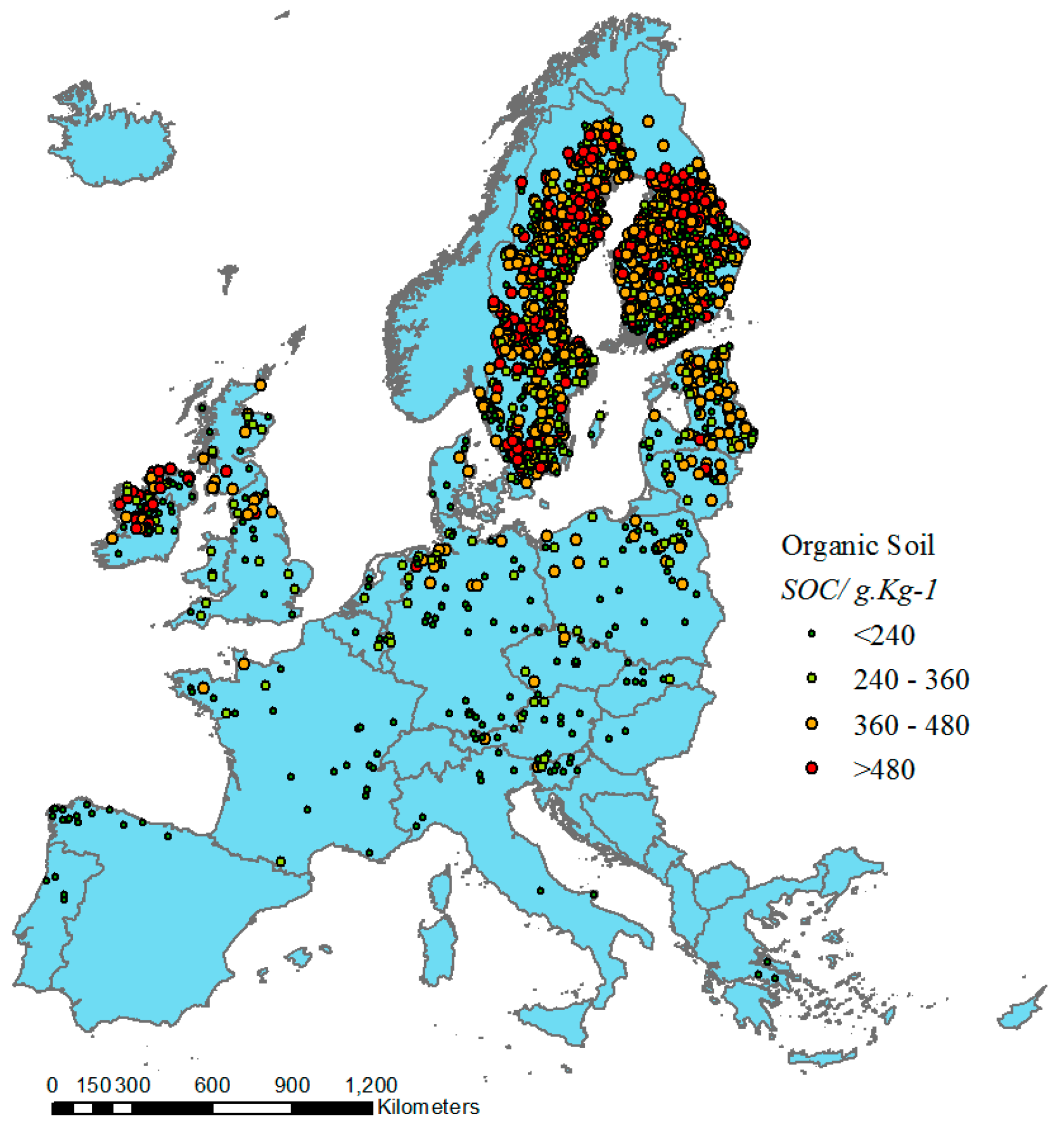
2.1. The LUCAS Topsoil Database

As part of Land Use/Land Cover Area Frame Survey, approximately 20,000 geo-referenced topsoil samples were collected and analysed for the 25 European Union member states [22,40]. Stratified random sampling was applied to collect around 0.5 kg of topsoil (0–20 cm) [41]. The collected samples can be classified as mineral and organic soils based on the extremely diverse spectral response. The LUCAS topsoil dataset is obtained from the Joint Research Centre (JRC) and can be used for non-commercial purposes [22]. In this paper, the proposed feature extraction method was tested using the LUCAS organic soil samples, the distribution of which was explored in ArcGIS 10.4 and can be seen in Figure 1.

The Vis-NIR-SWIR soil spectra were measured using a FOSS XDS Rapid Content Analyser (FOSS NIRSystems Inc., Denmark) [22], operating in the 400–2500 nm wavelength range, with 0.5 nm spectral resolution. Organic soil spectra were pre-processed by removing the data at wavelengths of 400–500 nm that showed instrumental artefacts, transformation of absorbance (A) spectra into reflectance (1/10^A) spectra, continuum removal, Savitzky-Golay filter with a window size of 50, second order polynomial and first derivative. Thirteen soil properties have been analysed in a central laboratory [22], including the percentage of coarse fragments, particle size distribution (% clay, silt and sand content), pH (in CaCl₂ and H₂O), soil organic carbon (g/kg), carbonate content (g/kg), phosphorous content (mg/kg), total nitrogen content (g/kg), extractable potassium content (mg/kg), and cation exchange capacity (cmol(+)/kg). Three key soil fertility properties, soil organic carbon (SOC), total nitrogen content (N) and pH in CaCl₂ (pH), were selected as our studied properties.

2.2. Fractal Feature Extraction Method

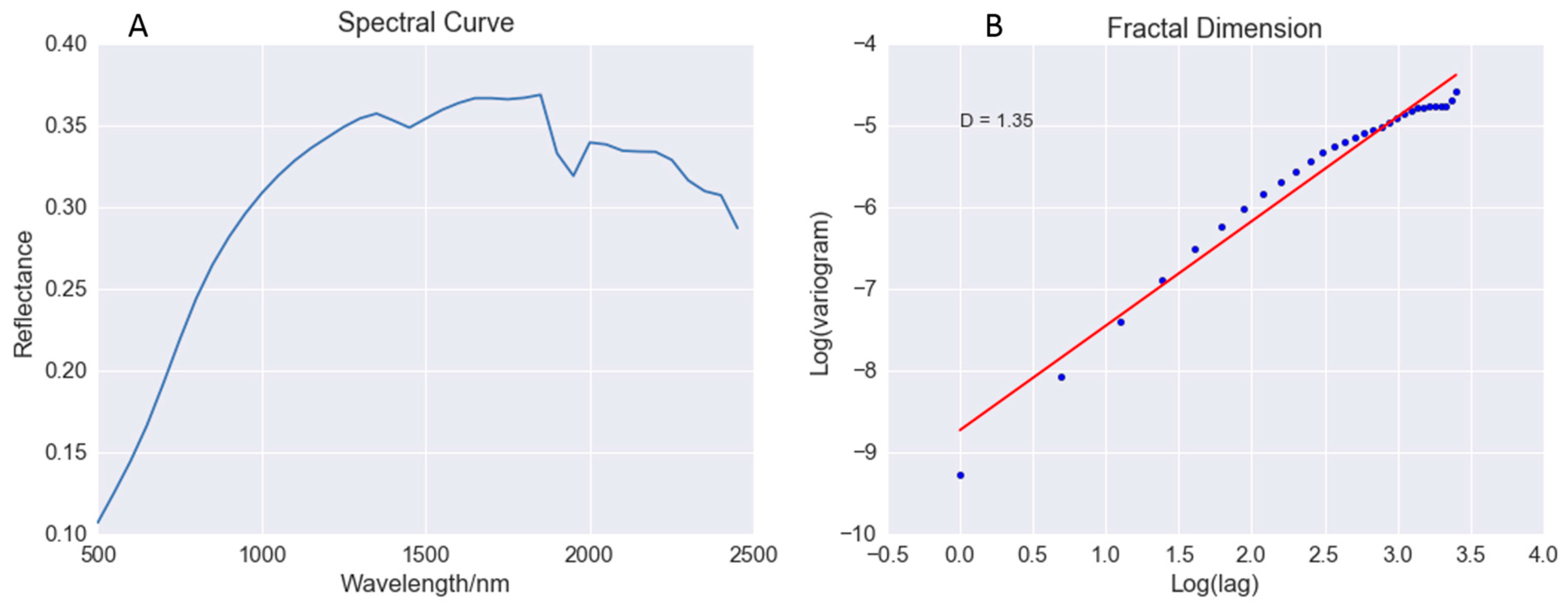
2.2.1. Concept of Fractal Dimension

Fractal dimension is a robust method for describing natural or man-made fractals having the fundamental feature known and referred to as self-similarity [42]. Within the fractal lies another copy of the same fractal, smaller but complete. If we have a strictly self-similar fractal which can be decomposed into N pieces, each of which is a copy of the original fractal scaled by a factor of $S$, then,

$$S^D=\mathrm{N}$$

(1)

where $D$ is the Hausdorff Dimension. $D$ is a non-integer number, describing how the irregular structure of objects and/or phenomena is replicated in an iterative way from small to large scales. Anything that appears random and irregular can be a fractal, strictly or statistically, including the soil Vis-NIR-SWIR spectrum, which cannot be defined by any mathematical equation and is therefore considered as an irregular curve. There are numerous methods which have been developed for fractal dimension estimation, including box-count [43], variogram [44], power spectrum [24] and spectral [45] methods.

2.2.2. Variation Method for Fractal Dimension

The variogram estimator is widely used in the determination of the fractal dimension and it is known for its ease of use [46]. By sampling a large number of pairs of points along the spectral curve and computing the differences in their reflectance values, the fractal dimension is easily derived from the log–log plot of variogram and lags. X_u and X_t+u are two reflectance values located at points u and t+u, and these two points are separated by the lag of t. The variogram can be calculated as the mean sum of squares of all differences between pairs of values with a given distance divided by two.

$$\mathsf{\gamma }\left(t\right)=\frac{1}{2}E{(X_u-X_{t+u})}^2$$

(2)

The variogram estimator is a stochastic process with stationary increments as half times the expectation of the square of an increment at lag t, and a generalisation of the variation estimator can be obtained with different order p of a stochastic process [47]:

$${\mathsf{\gamma }}_p\left(t\right)=\frac{1}{2}E|X_u-X_{t+u}{|}^p$$

(3)

where p = 1.0, it represents the madogram, which instead of calculating squares of the differences takes the absolute values. Where p = 1/2, the rodogram is derived by calculating the square root of absolute differences. Fractal dimension is estimated using the slope ($\theta$) of the corresponding log–log regression plot of ${\mathsf{\gamma }}_p\left(t\right)$ and t, as shown in Figure 2.

$$D=2-\frac{\theta }{2}$$

(4)

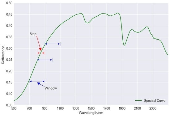
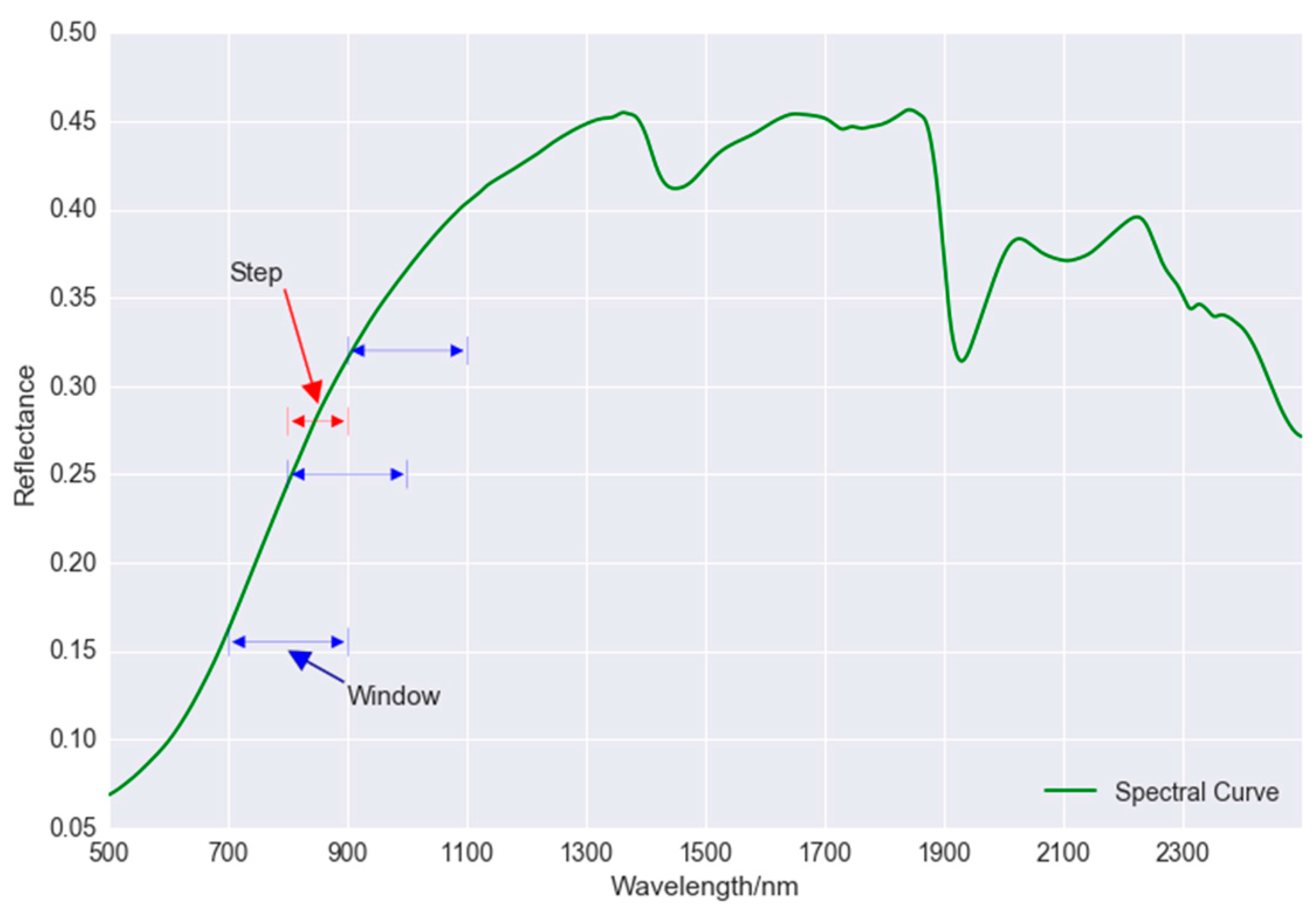
2.2.3. Fractal Feature Generation

Fractal features are generated by multiplying spectral energy with the corresponding fractal dimension. As the fractal dimension can be calculated using the whole curve or only part of the curve, the spectrum can be segmented into several parts and each part corresponds to a new fractal feature. For a soil spectral curve, a common approach is to evenly divide the whole curve into a desired number of segments [48], which means the step and window size are the same. In this study, we explored the effect of different combinations of step and window sizes on generated fractal features. The final feature number N_f can be calculated as:

$$N_f=\frac{N_r-W}{P}+1$$

(5)

$N_r$ is the number of raw spectral measurements, $P$ is the value of step size and W is the value of moving window size. W is obtained by multiplying scale and step value. It should be pointed out that the scale here is not the scaling factor for fractal dimension. When the window size is equal to the scale size, the fractal dimension of the spectral segment is calculated using reflectance values within the same wavelength window. The window size is often defined as larger than the step size, which means segments of the same spectral curve are overlapping. Step size is defined as 100.0 nm and moving window size as 200.0 nm, as shown in Figure 3, which means $P$ = 200 and w = 400 (the spectral resolution is 0.5 nm in our case). New fractal features can be generated when the wavelength window moves along the spectral curve at step 100.0 nm. With the increase of the step size, the final fractal feature number (N_f) correspondingly decreases, which can be used as a means of dimension reduction.

For a certain scale value, s, N_f numbers of fractal dimension values can be obtained by moving along the spectral curve at step size p. For each segment, the number of points are marked as n and can be calculated by Equation (5). The reflectance value as Z_j (j = 1, 2,…, n) and the corresponding fractal dimension value can be calculated according to Equation (4) as D_m (m = 1, 2,…, N_f), and fractal features at scale s by:

$$F_m={\mathrm{D}}_m\times {\mathrm{E}}_m$$

(6)

where ${\mathrm{E}}_m$ is the spectral energy and can be derived from the following equation:

$${\mathrm{E}}_m={\displaystyle \sum }_{j=1}^n{Z}_{m,j}^2$$

(7)

2.3. Gradient-Boosting Regression Model

Soil spectroscopy quantitatively correlates with soil properties, which supposes that fitting a regression model with features extracted from spectra will have good predictive accuracies with respect to soil continuous properties. Gradient-boosting is a highly effective and widely used machine-learning approach [49]. Gradient-boosting develops an ensemble of tree-based models by training each of the trees in the ensemble on different labels and then combining the trees. It can produce robust and interpretable procedures for both regression and classification. For a regression problem where the objective is to maximize the coefficient of determination (R²) or to minimize the root mean square error (RMSE), each successive tree is trained on the errors left over by the collection of earlier trees. XGBoost is a scalable and flexible gradient-boosting library [50,51,52], which is adopted to build the soil spectral quantitative model in our study. XGBoost uses more regularised model formalisation to control over-fitting, which gives it better performance. Mathematically, the model can be viewed as:

$${\widehat{y}}_i={\displaystyle \sum }_{k=1}^K{f}_k\left(x_i\right), f_k\in F$$

(8)

where $K$ is the number of trees, f is a function in the functional space $F$, and $F$ is the set of all possible regression trees. Therefore, the objective of optimization can be written as:

$$obj\left(\theta \right)={\displaystyle \sum }_i^{n}l(y_i,\widehat{y_i})+{\displaystyle \sum }_{k=1}^K\Omega \left(f_k\right)$$

(9)

where $l\left(y_i,\widehat{y_i}\right)$ is the training loss function, and $\Omega \left(f_k\right)$ is the regularization term. The goal of XGBoost model is to minimize $obj\left(\theta \right)$.

2.4. Evaluation

For each soil property, the soil spectral quantitative model was developed on a random sample of two-thirds of the selected soil samples using the gradient-boosting regression method. The calibrations were tested by predicting the soil properties on validation data sets composed of the remaining one-third of the organic soil samples. No samples were omitted from the analysis, nor the calibration or validation data sets. The model accuracies were evaluated on estimated and measured soil SOC, N and pH values using RMSE, R² and the ratio of percent deviation (RPD).

$$R^2=\frac{{{\displaystyle \sum }}_{i=1}^n{\left({\widehat{y}}_i-\overline{y}\right)}^2}{{{\displaystyle \sum }}_{i=1}^n{\left(Y_i-\overline{Y}\right)}^2}$$

(10)

$$\mathrm{RMSE}=\sqrt{\frac{1}{n}{{\displaystyle \sum }}_{i=1}^n{\left({\widehat{y}}_i-y_i\right)}^2}$$

(11)

$$\mathrm{RPD}=\frac{SD}{RMSE}$$

(12)

where n is the number of validation samples, y is the measured values, $\overline{y}$ is the mean of the measured values, and $\widehat{y}$ is the estimated values. RPD is the ratio of the standard deviation (SD) of the calibration data to the RMSE of the validation data [53]. An RPD <1.0 indicates a very poor model and its use is not recommended; an RPD between 1.0 and 1.4 indicates a poor model where only high and low values are distinguishable; an RPD between 1.4 and 1.8 indicates a fair model which may be used for assessment and correlation; RPD values between 1.8 and 2.0 indicate a good model where quantitative predictions are possible; an RPD between 2.0 and 2.5 indicates a very good, quantitative model, and an RPD >2.5 indicates an excellent model.

3. Results

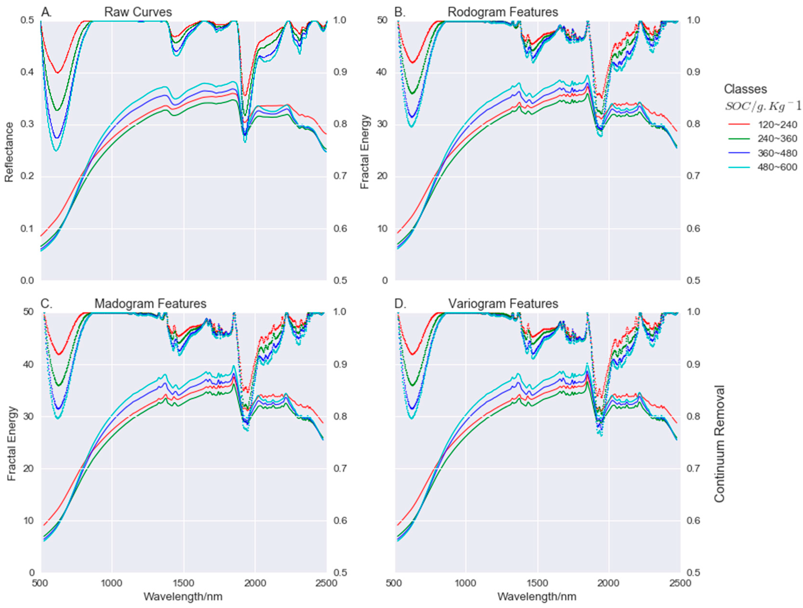
3.1. Fractal Features for Soil Spectroscopy

For a single soil Vis-NIR-SWIR spectrum, the fractal dimension can be calculated by Equation (4). Before extracting fractal features from soil spectra, we first examined the relationship between soil properties and the corresponding fractal dimension. Spectral values of soil are relatively low and the curve appears smoother compared with other objects like vegetation. Thus, the resulting fractal dimension values are comparatively low. Since the fractal dimension is derived from the slope of the regression line obtained from the log–log plot of γ_p(t) and lag t, one problem is how many lag increments are necessary to produce reliable results. Theoretically only a minimum of two points is necessary to make such a plot [46]. However, the results of such an analysis tend to not be reliable or representative. In this study, the value of lag increments was set as 5, and the Pearson correlations of soil properties and fractal dimensions are shown in

Table 1. Pearson correlation coefficients between soil properties and fractal dimensions calculated by rodogram, madogram and variogram estimators.

	Rodogram	Madogram	Variogram
SOC	−0.40	−0.47	−0.54
N	−0.38	−0.43	−0.50
pH	−0.12	−0.13	−0.12

. The Pearson is a standardized covariance and ranges from −1 to +1, which indicates a perfect negative (−1) or positive (+1) linear relationship respectively. A value of zero is not related to the independency between the two variables, it only suggests no linear association. It can be seen that SOC, N and pH have negative relationships with fractal dimension. SOC and N have similar correlations with fractal dimension. Among these three estimators, the variogram-based fractal dimension calculation method achieved the best correlation between fractal dimension values and soil properties SOC (correlation coefficient (r) = −0.54), N (r = −0.50) and pH (r = −0.12).

An intact spectrum can be divided into multiple segments, overlapping or non-overlapping. Each segment is corresponding to a fractal feature. When step size and window size are respectively set to 2.5 nm and 50.0 nm, a total number of 791 fractal features can be derived by rodogram, madogram or variogram methods, resulting the original spectral dimension reduced from 4000 to 791. In order to make a proper comparison between the generated fractal feature-based curve and the raw spectral curve, the centre wavelength value of the spectral segment is assigned to the fractal feature as the corresponding “wavelength number”.

A great advantage of fractal-based feature extraction is that the curve shape of fractal features is similar to the shape of raw spectrum, which makes it possible to apply methods like continuum removal (CR) not only to the raw spectrum but also to the fractal-based “spectrum”. The organic soil samples can be divided into four groups according to the content of SOC. Average spectral reflectance and continuum removal reflectance of LUCAS organic soil samples were computed by SOC classes (Figure 4A). For fractal features, average fractal energy and continuum removal responses of organic soil samples were also computed and shown in Figure 4B–D. The highest SOC class that was above 480 g/kg showed the highest mean reflectance in wavelength range from 1000.0 nm to 2000.0 nm, which is consistent with observations in the literature [4]. The continuum removal reflectance showed a strong correlation with SOC content at a wavelength of near 600.0 nm. The difference between raw spectral curve and fractal feature curve was not obvious from the view of shape. Fractal features showed shallow absorption peak in proportion for SOC classes at a wavelength of 600.0 nm. The fractal energy values were larger than reflectance values, as the former were multiplied by spectral energy and fractal dimension, which was supposed to be larger than 1.0.

To demonstrate the effects of step and window size on extracted fractal features, the combinations of the two parameters were tested. When the step size was fixed at 2.5 nm, a series of fractal feature curves were derived by defining window sizes as 15.0 nm, 35.0 nm, 55.0 nm, 75.0 nm and 95.0 nm. With the increase of window size, fractal energies correspondingly increased and the shapes of fractal features were also gradually exaggerated, as shown in Figure 5A. The number for fractal features derived at different window sizes were equal but less than raw spectral features. When the window size was fixed at 50.0 nm and step size increased from 10.0 to 50.0 nm at an interval of 7.5 nm, the number of fractal features was non-linearly decreased from 196 to 40 as shown in Figure 5B.

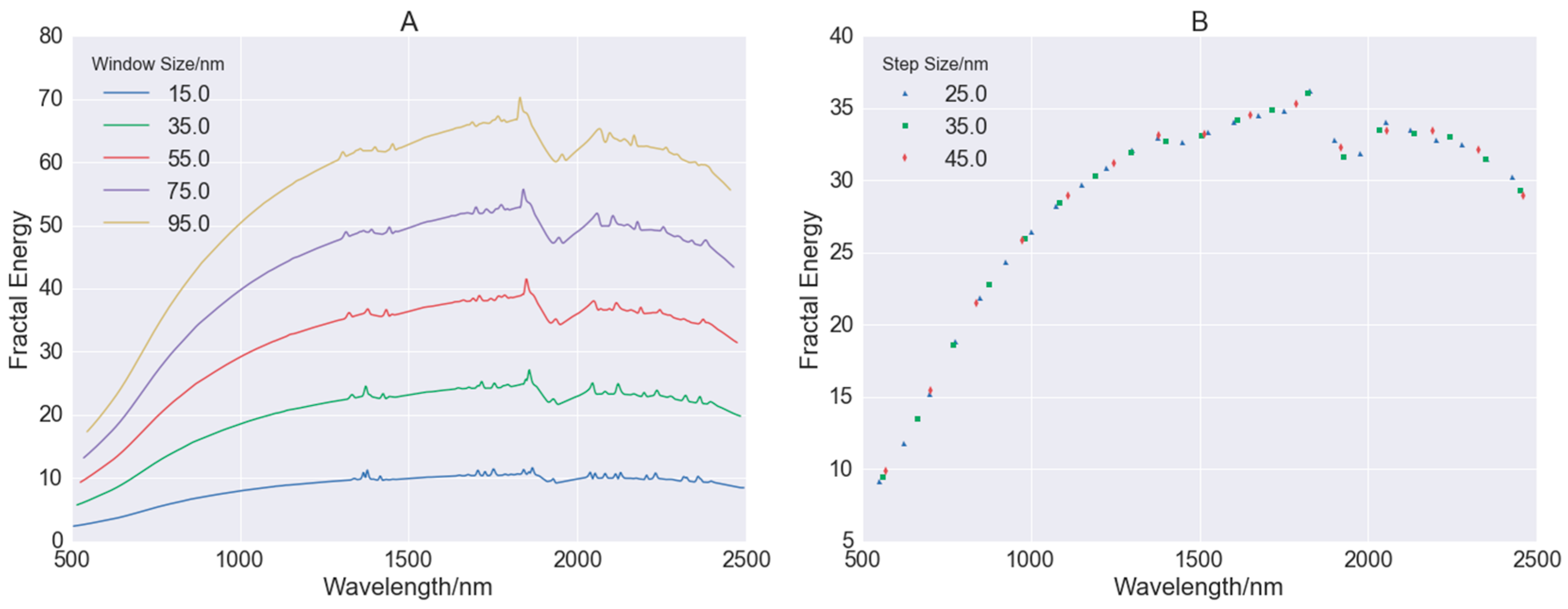
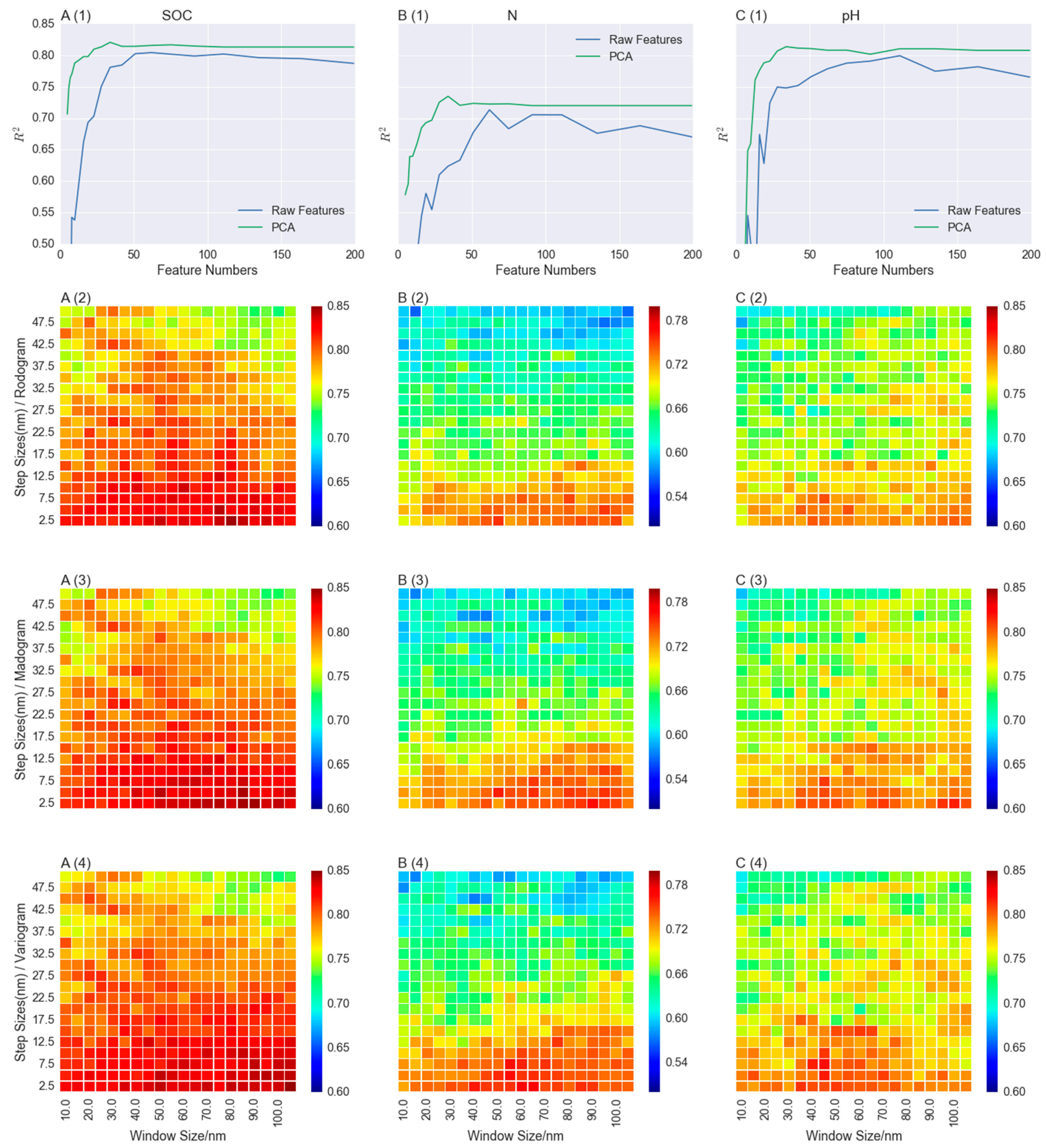
3.2. Effects of Different Step and Window Size on Extracted Fractal Features

For further analysis about effects of step and window size on the relationship between fractal features and soil properties, a matrix of step–window pairs was generated by defining step size ranging from 2.5 nm to 50.0 nm at an interval of 2.5 nm and window size ranging from 10.0 nm to 100.0 nm at an interval of 5.0 nm. For each pair of these two parameters, fractal features were derived according to Equation (6). A gradient-boosting regression model using the XGBoost tool was built on a random sample of two-thirds of organic soil samples, and then applied to the estimation of each sample from the validation dataset. Pre-processing methods for soil spectra could also be applied to new fractal features because of the shape similarity between fractal features and the raw spectral curve. For example, fractal features were smoothed by use of Savitzky-Golay filter. R² derived by step–window pairs for SOC using rodogram, madogram and variogram methods are shown in Figure 6(A2–A4) respectively, as is the case for N and pH in Figure 6B,C. For a comparable study, the regression model was also applied to raw spectral values and PCA-transformed data.

Taking advantage of fractal features, models developed for SOC estimation achieved comparably good results, R² varies from 0.64 to 0.83 (rodogram), 0.70 to 0.84 (madogram) and 0.72 to 0.84 (variogram). For pH, R² varies from 0.61 to 0.80 (rodogram), 0.63 to 0.80 (madogram) and 0.63 to 0.82 (variogram. However, for N there is comparatively less accuracy. R² varies from 0.52 to 0.74 (rodogram), 0.53 to 0.75 (madogram) and 0.55 to 0.76 (variogram). Models with raw spectra were developed by evenly selecting desired number of spectral measurements. The Hughes phenomenon can be seen well in models built with raw spectra. R² increased first and then declined with the increase of feature numbers. It can be seen that models with raw spectra had the poorest performance. For SOC and N, fractal features outperformed PCA-transformed features and raw spectra. Fractal features for pH achieved similar accuracies compared to PCA-transformed features.

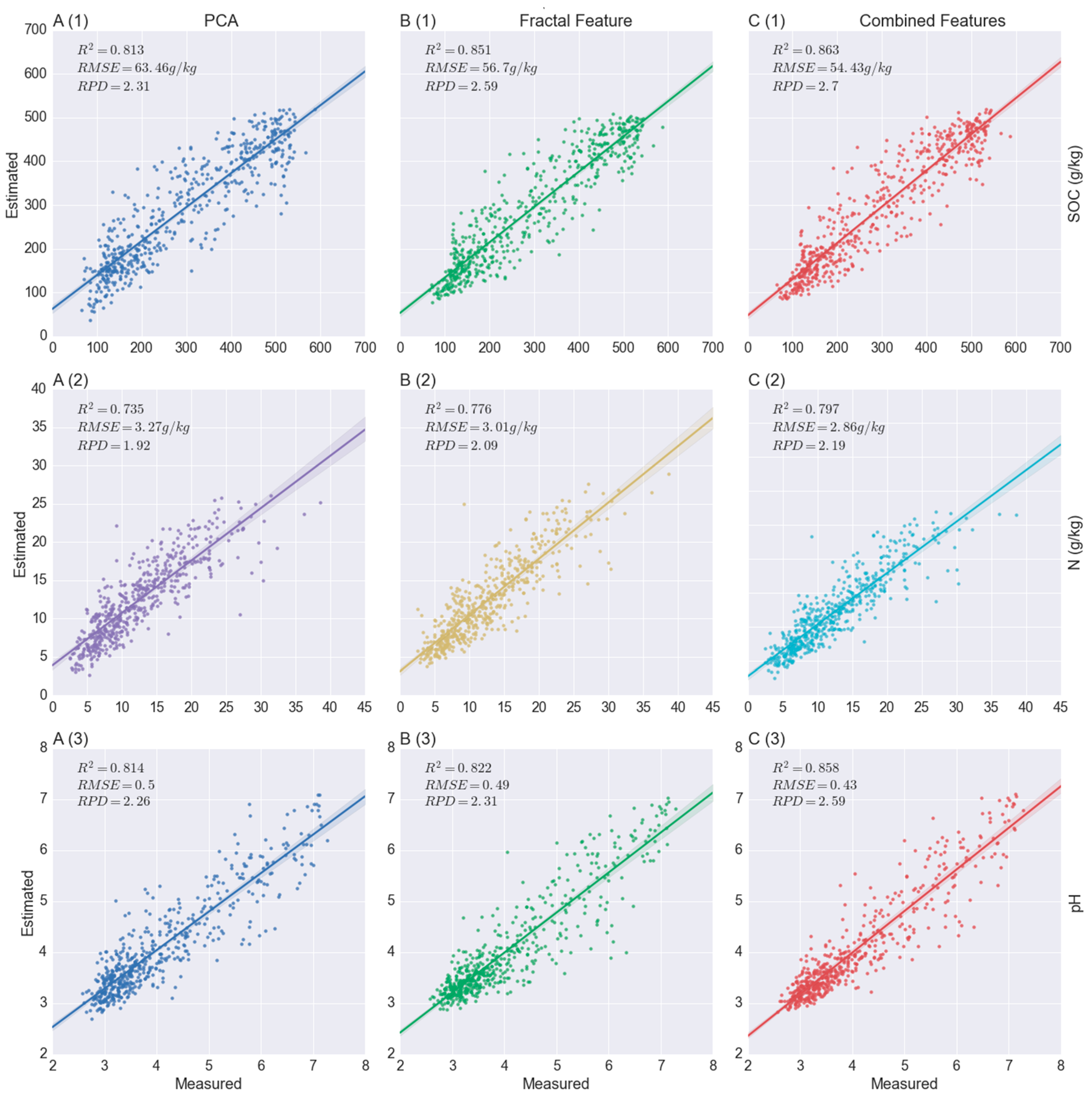
3.3. Modelling Soil Properties with Fractal Features

Window sizes and step sizes adopted to optimize the gradient-boosting regression model can be seen in Section 3.2. Fractal feature numbers approximately ranged from 40 to 800. The optimal pairs of step–window sizes for SOC, N and pH can be seen in

Table 2. Best Performance step–window pairs for soil properties estimation using fractal-based feature extraction and comparison with PCA. R²: coefficient of determination.

	Method	Step Size/nm	Window Size/nm	Dimension	R2
SOC	PCA	-	-	28	0.813
	Rodogram	2.5	80	769	0.847
	Madogram	2.5	90	765	0.847
	Variogram	2.5	105	759	0.851
N	PCA	-	-	34	0.735
	Rodogram	2.5	50	781	0.756
	Madogram	2.5	90	765	0.767
	Variogram	2.5	65	775	0.776
pH	PCA	-	-	34	0.814
	Rodogram	5	55	390	0.806
	Madogram	2.5	100	761	0.818
	Variogram	7.5	45	261	0.821

. For each gradient-boosting regression model built with XGBoost library, the maximum tree depth was 4 and maximum number of trees was 100. R² was used as the evaluation metric for validation data.

The best trade-off between step and window size for SOC (R² = 0.851, RMSE = 56.7 g/kg, RPD = 2.59) was 2.5 nm for the former and 105.0 nm for the latter with variogram estimator. The best performance step–window sizes for N (R² = 0.776, RMSE = 3.01 g/kg, RPD = 2.09) were step size at 2.5 nm and window size at 65.0 nm with the variogram estimator. The best performance step–window size for N (R² = 0.822, RMSE = 0.49, RPD = 2.31) were step size at 7.5 nm and window size at 45.0 nm with the variogram estimator. From Table 2, it can be seen that fractal-based feature extraction methods tend to keep a much larger number of features compared to PCA. To achieve similar performance of PCA, fractal-based approaches need to retain ~200 features, such as 190 for SOC (R² = 0.819, RMSE = 62.49 g/kg, RPD = 2.34) where step size and window size were respectively 10.0 nm and 105.0 nm, 128 features for N (R² = 0.736, RMSE = 3.26 g/kg, RPD = 1.92) where step size and window size were respectively 15.0 nm and 135.0 nm, and 131 features for pH (R² = 0.807, RMSE = 0.50, RPD = 2.22) where step size and window size were respectively 15.0 nm and 50.0 nm.

In real-world examples, there are many ways to extract features from a dataset. Often it is beneficial to combine several methods to obtain good performance. To assess whether predictive accuracy could be enhanced by integrating multiple features, the first 30 PCA components were combined with fractal features and then ingested into the gradient-boosting regression model. Combined features showed better performance when applied for the estimation of all three soil properties, SOC (R² = 0.86, RMSE = 55.16 g/kg, RPD = 2.7), N (R² = 0.78, RMSE = 2.96 g/kg, RPD = 2.19) and pH (R² = 0.85, RMSE = 0.44, RPD = 2.59), as shown in Figure 7.

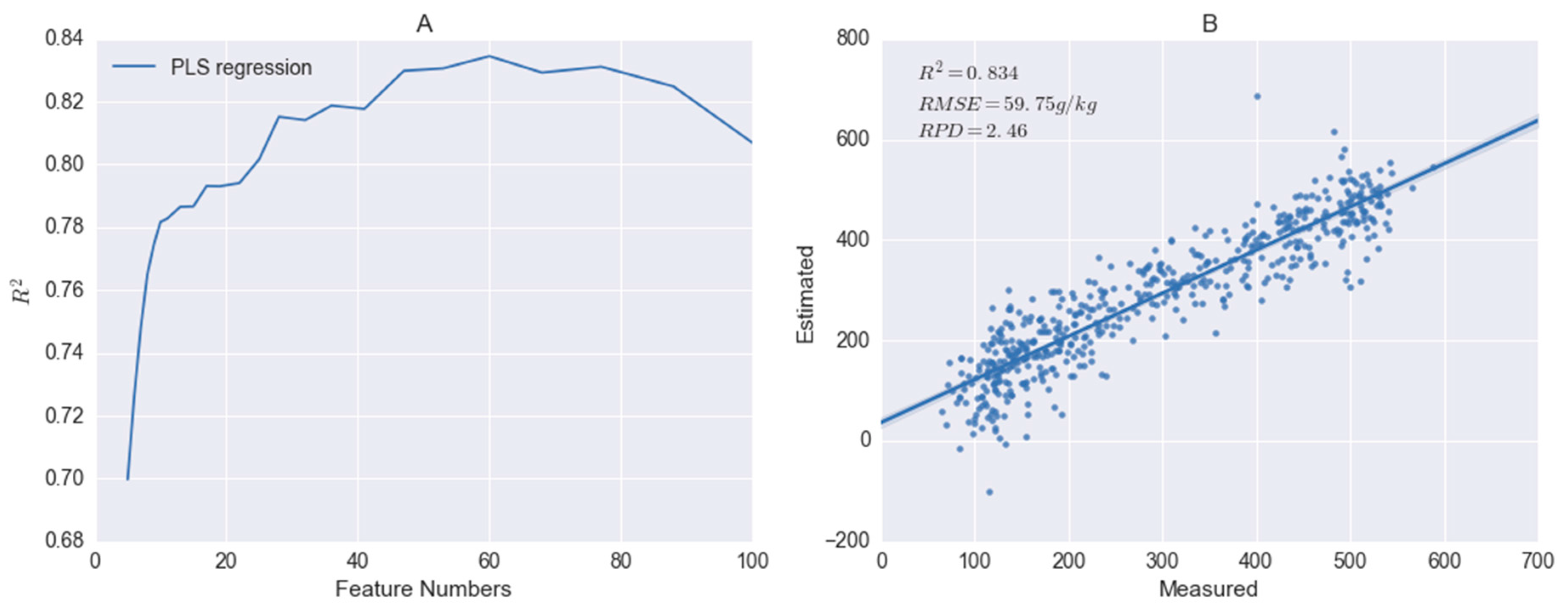
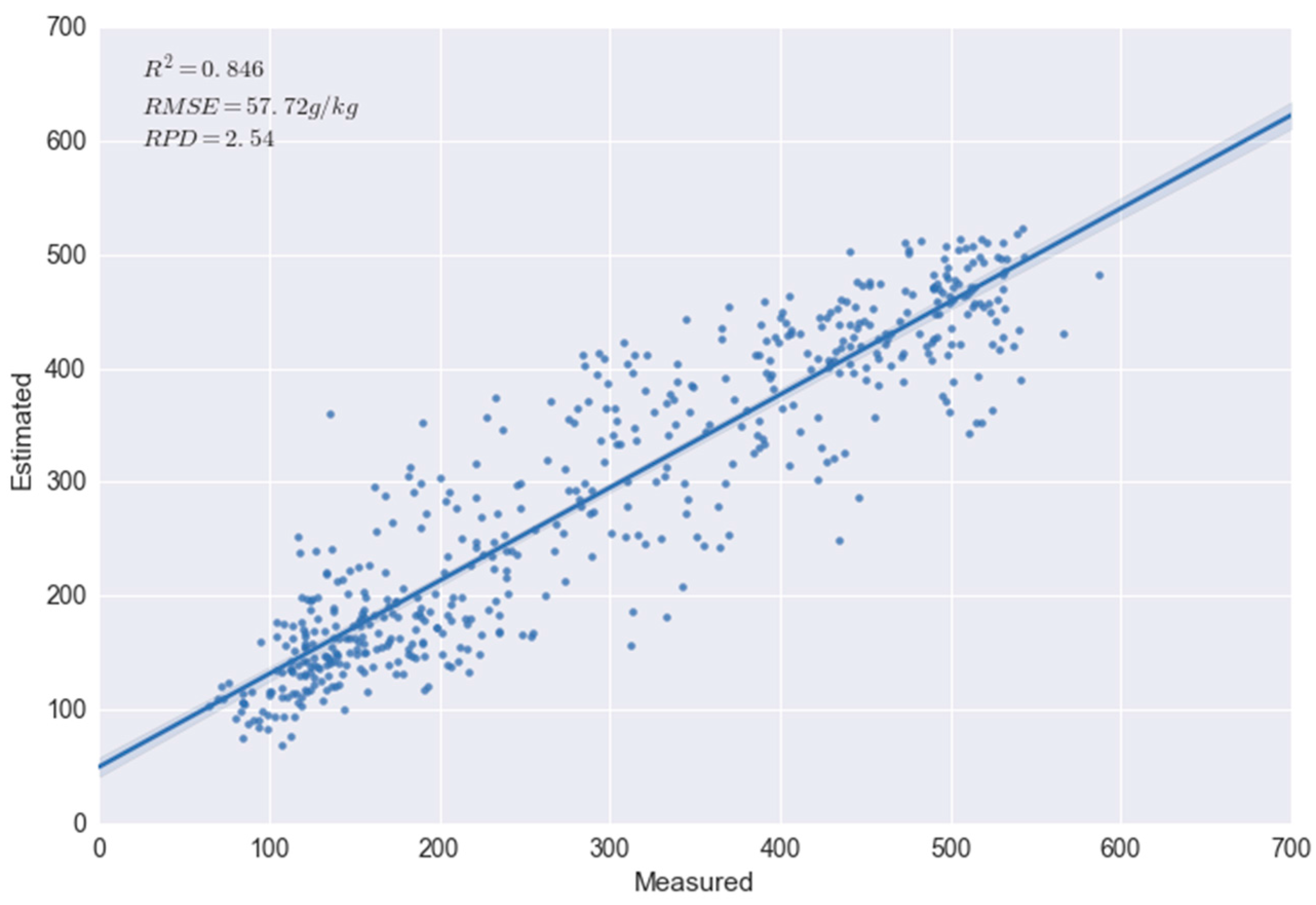
3.4. Comparison with PLS Regression

PLS regression is frequently used to calibrate soil properties with soil spectra, and it can maximize the covariance between the spectra and a measured soil property [7]. To make a comparison, PLS regression, named as method A for the sake of convenience, was applied to the raw spectra of the LUCAS organic soil to estimate organic carbon (OC) contents, and the best performance (R² = 0.834) was achieved when the number of components was 60 (Figure 8).

PLS regression integrates the compression and regression steps, and it can be viewed as a combination of PLS components and linear regression [54]. Therefore, it is also possible to transform the raw spectra into PLS components and then ingest them into the gradient-boosting regression model (method B). The same gradient-boosting model parameters were adopted. When the number of retained PLS components was 60, the achieved R² for the estimation of OC contents was 0.846 (Figure 9).

The quantitative method proposed in the paper can be viewed as a combination of fractal features and gradient-boosting regression (method C), and it achieved the best performance (R² = 0.851) for the estimation of SOC contents of these three methods. We also applied methods A and B to the estimation of N and pH contents. For N, the same case applied; method C showed the highest R². Although method A (PLS regression) achieved the best performance for the estimation of pH contents, when focusing on extracted features, fractal features had similar performance compared with PLS components, the R² for method C being 0.821 and for method B, 0.823. The only difference between these two methods was the ingested features. The results are summarised in

Table 3. Comparison of three methods for the quantitative retrieval of soil properties.

	Features	Modelling	OC (R2)	N (R2)	pH (R2)
Method A	PLS components	Linear regression	0.834	0.743	0.87
Method B	PLS components	Gradient-boosting regression	0.846	0.759	0.823
Method C	Fractal features	Gradient-boosting regression	0.851	0.776	0.821

, and it can be seen that fractal features can achieve similar or even better results compared with PLS components.

4. Discussion

4.1. The Importance of Fractal Dimension for Soil Spectra

The correlations between fractal dimension and soil properties were assessed by means of Pearson correlation analysis when the fractal dimension calculation was applied to the whole spectrum. Significant negative correlations for SOC (r = −0.54) and N (r = −0.50) with the fractal dimension were found, which means that values of SOC and N could have effects on the shape of soil spectra and therefore diagnostic wavelengths exist for SOC and N. In [55] an absorption peak centred at 600 nm was observed, which seems to be related to SOC content. At 2100 nm, there was an absorption determined by N content. In [4] the authors also highlighted that wavelengths of around 1100, 1600, 1700–1800, 2000, and 2200–2400 nm have been identified as being particularly important for SOC and N estimation.

The pH showed a very weak correlation with the fractal dimension (r = −0.12), which could be caused by a lower direct spectral response to soil pH [4]. It has to be pointed out that the weak correlation between pH and fractal dimension does not mean that soil spectra cannot be used to quantify soil pH values, but means that the variation of soil pH values does not significantly contribute to the smoothness or roughness of the spectral curve. Soil pH value can still be well estimated in the laboratory or in the field [55,56] using raw spectral data, which might be due to the mutual effect of spectrally active soil constituents such as organic matter and clay [57]. It also can be seen that the Pearson correlation between fractal dimension and soil properties has a positive relationship with the performance of fractal features.

4.2. Modelling Soil Properties with Fractal Features

Three methods for the fractal dimension calculation and further feature extraction were studied in this paper. The results demonstrate that the variogram estimator had slightly better performance than the madogram estimator when applied to fractal feature generation for soil property estimation, and methods using these two estimators achieved better R² than the method using the rodogram estimator. In [58] the classification achieved better results with texture layers derived from the madogram. Since the madogram estimator calculates the sum of the absolute value of the semivariance for all observed lags, it yields a softer effect on the presence of outliers compared to the variogram estimator. However, in our study, soil spectra were well pre-processed by the Savitzky–Golay filter and generated fractal features. Fractal features generated by these three estimators have a similar curve shape and achieved very close estimation accuracies for tested soil properties.

Step–window pairs have significant impact on estimation accuracies of soil properties. When the window size is fixed, accuracies are decreased with the increase of step size. However, when the step size is fixed, accuracies are prone to ascend slightly and then clearly descend. A higher R² was found to be located at the bottom of the step–window matrix. However, there is no guarantee as to which step–window pair is the best parameter for soil property estimation. Therefore, a hyper-parameter optimisation method should be adopted for each of the soil properties.

In general, fractal features achieved better results compared to PCA-transformed features and raw spectra. This demonstrates that by taking advantage of fractal information encoded in the soil spectral shape, soil properties can be estimated in a better way. Besides, when raw data are transformed or projected via PCA, measurement units and shape are lost. However, fractal-based feature extraction is prone to retaining much larger number of features compared to PCA. To achieve similar performance, the fractal-based approach needs ~200 feature numbers while PCA only needs ~30. When compared with PLS components, fractal features also had better performance for the estimation of OC and N contents. However, there is no conflict between common feature extraction practices with the proposed fractal method. When integrating different kinds of features, like PCA-transformed features and fractal features, the performance is expected to be improved for the retrieval of soil properties.

5. Conclusions

Data acquisition with Vis-NIR-SWIR spectroscopy is relatively easy, and a wide range of soil properties can be analysed within a comparatively short time with relatively little effort for sample preparation. Soil spectroscopy has recently been identified as a method that has the potential to rapidly estimate soil properties. Many soil-spectral libraries are already built at regional, continental or even global scales. Various multivariate statistics methods have been successfully adopted to explore the relationship between soil spectra and soil physical/chemical properties. However, few studies are focused on feature extraction from measured soil spectra, which is also crucial to correlating spectra with soil properties.

The present study presents a novel methodology for feature extraction based on fractal geometry. Each Vis-NIR-SWIR spectrum can be divided into multiple segments by defining the moving window size and the step size. For each segmented spectral curve, the fractal dimension value was calculated using variation estimators. Fractal features, generated by multiplying the fractal dimension value with spectral energy, were further combined with PCA-transformed features, and the gradient-boosting regression model achieved good performance with respect to the retrieval of SOC (R² = 0.86, RMSE = 55.16 g/kg, RPD = 2.7), N (R² = 0.78, RMSE = 2.96 g/kg, RPD = 2.19) and pH (R² = 0.85, RMSE = 0.44, RPD = 2.59). Fractal analysis can be functionalised as an approach to examine the relationship between soil spectra and soil properties, which can characterise statistical self-similarity and further quantify the irregularity of soil spectra [47]. Fractal features, by taking advantage of fractal information encoded in the shape of soil spectral curve, can reflect the impact of various properties on soil spectra except when the properties have less direct spectral response. In this case, fractal features can still be functioned to quantify the corresponding soil property, however, they not perform as well. Fractal features performed well when ingested into quantitative soil spectroscopic models, and the proposed fractal method can not only reduce the dimensionality in the original space, but also simultaneously maintain the spectral shape, which means that methods for raw spectra can also be applied to extracted fractal features, for example, calibrating soil properties using PLS regression with fractal features.

References

1. Viscarra Rossel, R.A.; Behrens, T.; Ben-Dor, E.; Brown, D.J.; Demattê, J.A.M.; Shepherd, K.D.; Shi, Z.; Stenberg, B.; Stevens, A.; Adamchuk, V.; et al. A global spectral library to characterize the world’s soil. Earth Sci. Rev. 2016, 155, 198–230. [Google Scholar] [CrossRef]
2. Stevens, A.; Nocita, M.; Tóth, G.; Montanarella, L.; van Wesemael, B. Prediction of soil organic carbon at the European scale by visible and near infraRed reflectance spectroscopy. PLoS ONE 2013, 8. [Google Scholar] [CrossRef] [PubMed]
3. Chabrillat, S.; Ben-Dor, E.; Viscarra Rossel, R.A.; Demattê, J.A.M. Quantitative soil spectroscopy. Appl. Environ. Soil Sci. 2013, 2013, 616578. [Google Scholar] [CrossRef]
4. Stenberg, B.; Viscarra Rossel, R.A.; Mouazen, A.M.; Wetterlind, J. Visible and near infrared spectroscopy in soil science. Adv. Agron. 2010, 107, 163–215. [Google Scholar]
5. Nocita, M.; Stevens, A.; van Wesemael, B.; Aitkenhead, M.; Bachmann, M.; Barthès, B.; Ben-Dor, E.; Brown, D.J.; Clairotte, M.; Csorba, A.; et al. Soil spectroscopy: An alternative to wet chemistry for soil monitoring. Adv. Agron. 2015, 132, 139–159. [Google Scholar]
6. Ben-Dor, E.; Taylor, R.G.; Hill, J.; Demattê, J.A.M.; Whiting, M.L.; Chabrillat, S.; Sommer, S. Imaging spectrometry for soil applications. Adv. Agron. 2008, 97, 321–392. [Google Scholar]
7. Rossel, R.A.V.; Behrens, T. Using data mining to model and interpret soil diffuse reflectance spectra. Geoderma 2010, 158, 46–54. [Google Scholar] [CrossRef]
8. Ramirez-Lopez, L.; Behrens, T.; Schmidt, K.; Stevens, A.; Demattê, J.A.M.; Scholten, T. The spectrum-based learner: A new local approach for modeling soil Vis-NIR spectra of complex datasets. Geoderma 2013, 195, 268–279. [Google Scholar] [CrossRef]
9. Soriano-Disla, J.M.; Janik, L.J.; Viscarra Rossel, R.A.; MacDonald, L.M.; McLaughlin, M.J. The performance of visible, near-, and mid-infrared reflectance spectroscopy for prediction of soil physical, chemical, and biological properties. Appl. Spectrosc. Rev. 2014, 49, 139–186. [Google Scholar] [CrossRef]
10. Epema, G.F.; Kooistra, L.; Wanders, J. Spectroscopy for the assessment of soil properties in reconstructed river floodplains. In Proceedings of the 3rd EARSeL Workshop on Imaging Spectroscopy, Herrsching, Germany, 13–16 May 2003; pp. 13–16.
11. Udelhoven, T.; Emmerling, C.; Jarmer, T. Quantitative analysis of soil chemical properties with diffuse refectance spectrometry and partial least-square regression: A feasibility study. Plant Soil 2003, 251, 319–329. [Google Scholar] [CrossRef]
12. McBratney, A.B.; Minasny, B.; Viscarra Rossel, R.A. Spectral soil analysis and inference systems: A powerful combination for solving the soil data crisis. Geoderma 2006, 136, 272–278. [Google Scholar] [CrossRef]
13. Shepherd, K.D.; Walsh, M.G. Infrared spectroscopy—Enabling an evidence-based diagnostic surveillance approach to agricultural and environmental management in developing countries. J. Near Infrared Spectrosc. 2007, 15, 1–19. [Google Scholar] [CrossRef]
14. Tóth, G.; Hermann, T.; Da Silva, M.R.; Montanarella, L. Heavy metals in agricultural soils of the European Union with implications for food safety. Environ. Int. 2016, 88, 299–309. [Google Scholar] [CrossRef] [PubMed]
15. Viscarra Rossel, R.A.; Walvoort, D.J.J.; McBratney, A.B.; Janik, L.J.; Skjemstad, J.O. Visible, near infrared, mid infrared or combined diffuse reflectance spectroscopy for simultaneous assessment of various soil properties. Geoderma 2006, 131, 59–75. [Google Scholar] [CrossRef]
16. Ji, W.; Li, S.; Chen, S.; Shi, Z.; Viscarra Rossel, R.A.; Mouazen, A.M. Prediction of soil attributes using the Chinese soil spectral library and standardized spectra recorded at field conditions. Soil Tillage Res. 2016, 155, 492–500. [Google Scholar] [CrossRef]
17. Guanter, L.; Kaufmann, H.; Segl, K.; Foerster, S.; Rogass, C.; Chabrillat, S.; Kuester, T.; Hollstein, A.; Rossner, G.; Chlebek, C.; et al. The EnMAP spaceborne imaging spectroscopy mission for earth observation. Remote Sens. 2015, 7, 8830–8857. [Google Scholar] [CrossRef]
18. Goetz, A.F.; Vane, G.; Solomon, J.E.; Rock, B.N. Imaging spectrometry for earth remote sensing. Science 1985, 228, 1147–1153. [Google Scholar] [CrossRef] [PubMed]
19. Green, R.O.; Eastwood, M.L.; Sarture, C.M.; Chrien, T.G.; Aronsson, M.; Chippendale, B.J.; Faust, J.A.; Pavri, B.E.; Chovit, C.J.; Solis, M.; et al. Imaging spectroscopy and the Airborne Visible/Infrared Imaging Spectrometer (AVIRIS). Remote Sens. Environ. 1998, 65, 227–248. [Google Scholar] [CrossRef]
20. Franceschini, M.H.D.; Demattê, J.A.M.; da Silva Terra, F.; Vicente, L.E.; Bartholomeus, H.; de Souza Filho, C.R. Prediction of soil properties using imaging spectroscopy: Considering fractional vegetation cover to improve accuracy. Int. J. Appl. Earth Obs. Geoinf. 2015, 38, 358–370. [Google Scholar] [CrossRef]
21. Steinberg, A.; Chabrillat, S.; Stevens, A.; Segl, K.; Foerster, S. Prediction of common surface soil properties based on Vis-NIR airborne and simulated EnMAP imaging spectroscopy data: Prediction accuracy and influence of spatial resolution. Remote Sens. 2016, 8. [Google Scholar] [CrossRef]
22. Tóth, G.; Jones, A.; Montanarella, L. LUCAS Topsoil Survey: Methodology, Data, and Results; Joint Research Centre, European Commission: Ispra, Italy, 2013. [Google Scholar]
23. Vågen, T.G.; Shepherd, K.D.; Walsh, M.G.; Winowiecki, L.; Desta, L.T.; Tondoh, J.E. AfSIS Technical Specifications: Soil Health Surveillance; World Agroforestry Centre: Nairobi, Kenya, 2010. [Google Scholar]
24. Mukherjee, K.; Ghosh, J.K.; Mittal, R.C. Dimensionality reduction of hyperspectral data using spectral fractal feature. Geocarto Int. 2012, 27, 515–531. [Google Scholar] [CrossRef]
25. Huang, H.; Luo, F.; Liu, J.; Yang, Y. Dimensionality reduction of hyperspectral images based on sparse discriminant manifold embedding. ISPRS J. Photogramm. Remote Sens. 2015, 106, 42–54. [Google Scholar] [CrossRef]
26. Qiao, T.; Ren, J.; Craigie, C.; Zabalza, J.; Maltin, C.; Marshall, S. Quantitative prediction of beef quality using visible and NIR spectroscopy with large data samples under industry conditions. J. Appl. Spectrosc. 2015, 82, 137–144. [Google Scholar] [CrossRef]
27. Xing, C.; Ma, L.; Yang, X. Stacked denoise autoencoder based feature extraction and classification for hyperspectral images. J. Sensors 2015, 2016, 3632943. [Google Scholar] [CrossRef]
28. Li, F.; Xu, L.; Wong, A.; Clausi, D.A. Feature extraction for hyperspectral imagery via ensemble localized manifold learning. IEEE Geosci. Remote Sens. Lett. 2015, 12, 2486–2490. [Google Scholar]
29. Bakir, C. Nonlinear feature extraction for hyperspectral images. Int. J. Appl. Math. Electron. Comput. 2015, 3, 244–248. [Google Scholar] [CrossRef]
30. Lunga, D.; Prasad, S.; Crawford, M.M.; Ersoy, O. Manifold-learning-based feature extraction for classification of hyperspectral data: A review of advances in manifold learning. IEEE Signal Process. Mag. 2014, 31, 55–66. [Google Scholar] [CrossRef]
31. Rossel, R.A.V.; Chen, C. Digitally mapping the information content of visible-near infrared spectra of surficial Australian soils. Remote Sens. Environ. 2011, 115, 1443–1455. [Google Scholar] [CrossRef]
32. Zheng, L.; Li, M.; An, X.; Pan, L.; Sun, H. Spectral feature extraction and modeling of soil total nitrogen content based on NIR technology and wavelet packet analysis. SPIE Asia-Pac. Remote Sens. 2010, 7857. [Google Scholar] [CrossRef]
33. Ramirez-lopez, L.; Behrens, T.; Schmidt, K.; Viscarra Rossel, R.A.; Demattê, J.A.M.; Scholten, T. Distance and similarity-search metrics for use with soil vis-NIR spectra. Geoderma 2013, 199, 43–53. [Google Scholar] [CrossRef]
34. Bengio, Y.; Courville, A.; Vincent, P. Representation learning: A review and new perspectives. IEEE Trans. Pattern Anal. Mach. Intell. 2013, 35, 1798–1828. [Google Scholar] [CrossRef] [PubMed]
35. Roweis, S. Nonlinear dimensionality reduction by locally linear embedding. Science 2000, 290, 2323–2326. [Google Scholar] [CrossRef] [PubMed]
36. Kalousis, A.; Prados, J.; Rexhepaj, E.; Hilario, M. Feature extraction from mass spectra for classification of pathological states. In Proceedings of the 9th European Conference on Principles and Practice of Knowledge Discovery in Databases, Porto, Portugal, 3–7 October 2005.
37. Ghosh, J.K.; Somvanshi, A. Fractal-based dimensionality reduction of hyperspectral images. J. Indian Soc. Remote Sens. 2008, 36, 235–241. [Google Scholar] [CrossRef]
38. Junying, S.; Ning, S. A dimensionality reduction algorithm of hyper spectral image based on fract analysis. Int. Arch. Photogramm. Remote Sens. Spat. Inf. Sci. 2008, XXXVII, 297–302. [Google Scholar]
39. Mukherjee, K.; Bhattacharya, A.; Ghosh, J.K.; Arora, M.K. Comparative performance of fractal based and conventional methods for dimensionality reduction of hyperspectral data. Opt. Lasers Eng. 2014, 55, 267–274. [Google Scholar] [CrossRef]
40. Tóth, G.; Jones, A.; Montanarella, L. The LUCAS topsoil database and derived information on the regional variability of cropland topsoil properties in the European Union. Environ. Monit. Assess. 2013, 185, 7409–7425. [Google Scholar] [CrossRef] [PubMed]
41. Ballabio, C.; Panagos, P.; Monatanarella, L. Mapping topsoil physical properties at European scale using the LUCAS database. Geoderma 2016, 261, 110–123. [Google Scholar] [CrossRef]
42. Reljin, I.S.; Reljin, B.D.; Avramov-Ivić, M.L.; Jovanović, D.V.; Plavec, G.I.; Petrović, S.D.; Bogdanović, G.M. Multifractal analysis of the UV/VIS spectra of malignant ascites: Confirmation of the diagnostic validity of a clinically evaluated spectral analysis. Phys. A Stat. Mech. Its Appl. 2008, 387, 3563–3573. [Google Scholar] [CrossRef]
43. Hall, P.; Wood, A. On the performance of box-counting estimators of fractal dimension. Biometrika 1993, 80, 246–251. [Google Scholar] [CrossRef]
44. Constantine, A.G.; Hall, P. Characterizing surface smoothness via estimation of effective fractal dimension. J. R. Stat. Soc. Ser. B 1994, 56, 97–113. [Google Scholar]
45. Chan, G.; Hall, P.; Poskitt, D. Periodogram-based estimators of fractal properties. Ann. Stat. 1995, 1684–1711. [Google Scholar] [CrossRef]
46. Klinkenberg, B. A review of methods used to determine the fractal dimension of linear features. Math. Geol. 1994, 26, 23–46. [Google Scholar] [CrossRef]
47. Gneiting, T.; Sevcikova, H.; Percival, D.B. Estimators of fractal dimension: Assessing the roughness of time series and spatial data. Stat. Sci. 2011, 27, 247–277. [Google Scholar] [CrossRef]
48. Mukherjee, K.; Ghosh, J.K.; Mittal, R.C. Variogram fractal dimension based features for hyperspectral data dimensionality reduction. J. Indian Soc. Remote Sens. 2013, 41, 249–258. [Google Scholar] [CrossRef]
49. Friedman, J.H.J. Greedy function approximation: A gradient boosting machine. Ann. Stat. 2001, 29, 1189–1232. [Google Scholar] [CrossRef]
50. Song, R.; Chen, S.; Deng, B.; Li, L. eXtreme gradient boosting for dentifying individual users across different digital devices. In Proceedings of the 17th International Conference on Web-Age Information Management, Nanchang, China, 3–5 June 2016; pp. 43–54.
51. Chen, T.; Guestrin, C. XGBoost: Reliable large-scale tree boosting system. In Proceedings of the 22nd SIGKDD Conference on Knowledge Discovery and Data Mining, San Francisco, CA, USA, 13–17 August 2016; pp. 785–794.
52. Mustapha, I.B.; Saeed, F. Bioactive molecule prediction using extreme gradient boosting. Molecules 2016, 21. [Google Scholar] [CrossRef]
53. Viscarra Rossel, R.A.; McGlynn, R.N.; McBratney, A.B. Determining the composition of mineral-organic mixes using UV-Vis-NIR diffuse reflectance spectroscopy. Geoderma 2006, 137, 70–82. [Google Scholar] [CrossRef]
54. Höskuldsson, A. PLS regression methods. J. Chemom. 1988, 2, 211–228. [Google Scholar] [CrossRef]
55. Nocita, M.; Stevens, A.; Toth, G.; Panagos, P.; van Wesemael, B.; Montanarella, L. Prediction of soil organic carbon content by diffuse reflectance spectroscopy using a local partial least square regression approach. Soil Biol. Biochem. 2014, 68, 337–347. [Google Scholar] [CrossRef]
56. Kopačková, V. Using multiple spectral feature analysis for quantitative pH mapping in a mining environment. Int. J. Appl. Earth Obs. Geoinf. 2014, 28, 28–42. [Google Scholar] [CrossRef]
57. Wang, Y.; Huang, T.; Liu, J.; Lin, Z.; Li, S.; Wang, R.; Ge, Y. Soil pH value, organic matter and macronutrients contents prediction using optical diffuse reflectance spectroscopy. Comput. Electron. Agric. 2015, 111, 69–77. [Google Scholar] [CrossRef]
58. Wijaya, A.; Marpu, P.R.; Gloaguen, R. Geostatistical texture classification of tropical rainforest in Indonesia. In Proceedings of the 5th International Symposium for Spatial Data Quality (ISSDQ), Enschede, The Netherlands, 13–15 June 2007.
Figure 1. Distribution of organic soil samples in the Land Use/Land Cover Area Frame Survey (LUCAS) topsoil database. Colours indicate amounts of soil organic carbon (SOC) content.
Remotesensing 08 01035 g001
Figure 2. Illustration of fractal dimension calculation. (A) is the spectral curve and (B) is the corresponding log–log plot of variogram and lags and the fitted regression line.
Remotesensing 08 01035 g002
Figure 3. Illustration of the meaning of step and window size for multiple fractal feature generation. (step size = 100.0 nm, window size = 200.0 nm).
Remotesensing 08 01035 g003
Figure 4. (A) Average spectral reflectance and continuum removal reflectance of LUCAS organic soil samples computed by SOC classes. (BD) Average fractal energy and continuum removal responses of organic soil samples computed by SOC classes using rodogram, madogram and variogram estimators respectively. The central wavelength number of the corresponding spectral segment is assigned to the fractal feature.
Remotesensing 08 01035 g004
Figure 5. The effect of step and window size on generated fractal features. (A)are fractal feature curves when window sizes were at 15.0–95.0 nm (step size fixed at 2.5 nm); (B) is the number of fractal features when step sizes were increased from 10.0 to 50.0 nm (window size fixed at 50.0 nm).
Remotesensing 08 01035 g005
Figure 6. Gradient-boosting regression modelling accuracies for SOC, N and pH. (A1), (B1) and (C1) were with principal component analysis (PCA)-transformed features and raw spectra; (A2), (B2) and (C2) were with fractal features derived by the rodogram method with various step-scale pairs. (A3), (B3) and (C3) were with fractal features derived by the madogram method with various step-window pairs. (A4), (B4) and (C4) were with fractal features derived by the variogram method with various step-scale pairs.
Remotesensing 08 01035 g006
Figure 7. Best performance of gradient-boosting regression modelling accuracies for SOC, N and pH. (A1), (A2) and (A3) were with PCA-transformed features. (B1), (B2) and (B3) were with fractal features. (C1), (C2) and (C3) were with features combined by PCA-transformed features and fractal features. R2: coefficient of determination; RMSE: root mean square error; RPD: the ratio of percent deviation.
Remotesensing 08 01035 g007
Figure 8. The change of R2 with the increase of the partial least squares (PLS) component number (A) and the PLS regression model when the component number was 60 (B).
Remotesensing 08 01035 g008
Figure 9. The gradient-boosting regression model with PLS components for the estimation of OC contents.
Remotesensing 08 01035 g009