Evaluating the Potential of PROBA-V Satellite Image Time Series for Improving LC Classification in Semi-Arid African Landscapes

Abstract

Satellite based land cover classification for Africa’s semi-arid ecosystems is hampered commonly by heterogeneous landscapes with mixed vegetation and small scale land use. Higher spatial resolution remote sensing time series data can improve classification results under these difficult conditions. While most large scale land cover mapping attempts rely on moderate resolution data, PROBA-V provides five-daily time series at 100 m spatial resolution. This improves spatial detail and resilience against high cloud cover, but increases the data load. Cloud-based processing platforms can leverage large scale land cover monitoring based on such finer time series. We demonstrate this with PROBA-V 100 m time series data from 2014–2015, using temporal metrics and cloud filtering in combination with in-situ training data and machine learning, implemented on the ESA (European Space Agency) Cloud Toolbox infrastructure. We apply our approach to two use cases for a large study area over West Africa: land- and forest cover classification. Our land cover classification reaches a 7% to 21% higher overall accuracy when compared to four global land cover maps (i.e., Globcover-2009, Cover-CCI-2010, MODIS-2010, and Globeland30). Our forest cover classification shows 89% correspondence with the Tropical Ecosystem Environment Observation System (TREES)-3 forest cover data which is based on spatially finer Landsat data. This paper illustrates a proof of concept for cloud-based “big-data” driven land cover monitoring. Furthermore, we show that a wide range of temporal metrics can be extracted from detailed PROBA-V 100 m time series data to continuously optimize land cover monitoring.

1. Introduction

Semi-arid ecosystems with typically heterogeneous landscapes consisting of mixed vegetation (mosaics of trees, shrubs, and grassland) and small scale land use patterns pose challenges (e.g., mixed pixels) for remote sensing (RS) based medium resolution land cover (LC) mapping [1,2]. This is reflected by relatively low map accuracies in medium resolution (250–500 m) global LC datasets for those areas [3,4]. In a comparison of four recent global LC datasets over Africa, Tsendbazar et al. [5] found that for all reviewed maps, the areas of lowest correspondence with the reference data were the Sahel and dry savannah regions (see Figure 1), with high confusion between grass-, shrub-, and cropland classes.

Huttich et al. [1] show that the mapping accuracy for these classes can be improved by using dense multi-annual imagery time series: longer observation periods take inter-seasonal variability into account, while finer temporal resolution can help to better identify seasonal vegetation patterns. They find the highest mapping accuracies for sub-monthly observation frequencies over multi-annual periods. Additionally, dense time series can improve cloud masking by enabling the use of temporal filtering algorithms, while enough valid observations remain to derive temporal metrics even for the cloudy season [6,7]. Data records with lower temporal density such as Landsat can often not provide enough observations to allow the application of such techniques, especially in tropical areas with pronounced cloud cover [8].

Time series based LC classification requires new datasets and approaches: until 2014 only moderate or coarser spatial resolution sensors (e.g., Moderate Resolution Imaging Spectroradiometer (MODIS)) delivered regular observations at sub-monthly frequencies. Current large scale LC datasets mostly rely on those 250–500 m resolution datasets or are based on a few observations of Landsat-like data [5]. Only for forest cover (FC) is a global dataset based on long time series available [9], realized through processing on a large cloud-based computing platform.

The PROBA-V mission provides daily and five-daily-composite observations at 100 m spatial resolution [10]; the five-daily data provides almost complete coverage, while the daily data has large gaps. This finer resolution can be seen as an intermediate step towards the Sentinel 2 time series and provides higher spatial resolution data compared with other sensors such as MODIS, yet it keeps the temporal detail. By now almost three years of PROBA-V observations at 100 m spatial resolution are available, and the record is growing steadily. PROBA-V time series have been used successfully for cropland mapping in the Sahel region [11], and the 100 m resolution has been shown to improve crop type classification compared to the 300 m data [12].

The larger datasets at finer resolution call for scalable processing platforms and modular approaches that allow us to plug-in different training datasets and algorithms.

Here we present a proof of concept for a LC monitoring approach suitable for large-areas, based on temporal metrics from PROBA-V 100 m time series, in combination with temporal cloud filtering, in-situ training data, and machine learning. In two use cases, we apply this concept on LC and FC classification for a large study site in West Africa. Temporal metrics from the PROBA-V time series of 2014–2015 were classified using Random Forest (RF) and training data presented in [5] and from the Tropical Ecosystem Environment Observation System (TREES)-3 project [12,13]. The results were cross-validated and were also compared to existing datasets. The processing of the large datasets is realized through a cloud computing platform provided by European Space Agence (ESA) Research and Service Support [14].

2. Materials and Methods

2.1. Satellite Data

We use PROBA-V data with 100 m ground resolution provided as top-of-canopy reflection in a five-daily product acquired between March 2014 and October 2015. The study area covers four PROBA-V tiles (X16Y06–X19Y06, 20°W–20°E, 5°–15°N, see Figure 1). The PROBA-V data is provided with a pixel-state mask (SM) including cells identified as covered by cloud and cloud-shadow based on radiometric thresholds and sun-sensor geometry [10]. Noting that re-processing of the PROBA-V data with improved cloud detection is planned for 2016 [15], we used the data (Version 0) as provided in December 2015. The data compromises blue, red, near infrared (NIR), and shortwave infrared (SWIR) as top-of-canopy reflectance and normalized difference vegetation index (NDVI). The products are available through [16].

2.2. Training and Reference Data

For training and reference we used two datasets, based on which we prepared two classification use cases for the study area:

• An integrated LC reference dataset derived from existing datasets available through the Global Observation for forest cover and Land Dynamics (GOFC-GOLD) reference data portal and Geo-Wiki platform [17,18], as described in [5].
• The TREES-3 dataset, prepared by the Joint Research Center (JRC) of the European Commission as continuation of a record carried out in coordination with the United Nations Food and Agricultural Organization for their Global Forest Resource Assessment 2010 [13].

The integrated LC datasets consist of 708 samples for our study area. The dataset has nine LC classes: forest, shrubland, grassland, cropland including mixtures, wetland vegetation, bare/sparse-vegetation, urban/built-up, water, and snow/ice. The description of the legend and the corresponding LC classes of the reference datasets can be found in [19]. The latter three classes were underrepresented in the study area and were excluded from the classification. These datasets were mostly collected between 2000 and 2010 [5]. Although there is a temporal mismatch compared to the RS-data, the LC changes are relatively small compared to the inaccuracies in existing LC maps. Because of the relative small size of the dataset, we used all points for training and reported the out-of-bag (OOB) accuracies. OOB uses n-bootstrap datasets, leaving out one observation at a time for prediction. This approach has been shown to be comparable to error estimation from independent test data [20,21]. We compared the outcome of this use case with four recent global LC maps: (a) Land Cover-CCI; (b) Globeland30; (c) MODIS 2010; and (d) Globcover-2009, along with (e) a regression kriging based integrated LC map of (a)–(d) presented in [5].

The TREES-3 dataset is based on a classification for Landsat data 10 × 10 km tiles at every confluence of degrees. It has 6 thematic FC classes: tree cover >70%, mosaic (tree cover 30%—70%), other wooded land, other vegetation, bare and water. We used ten percent of the data for training and validated against the remaining 90%, based on a random sample stratified by class.

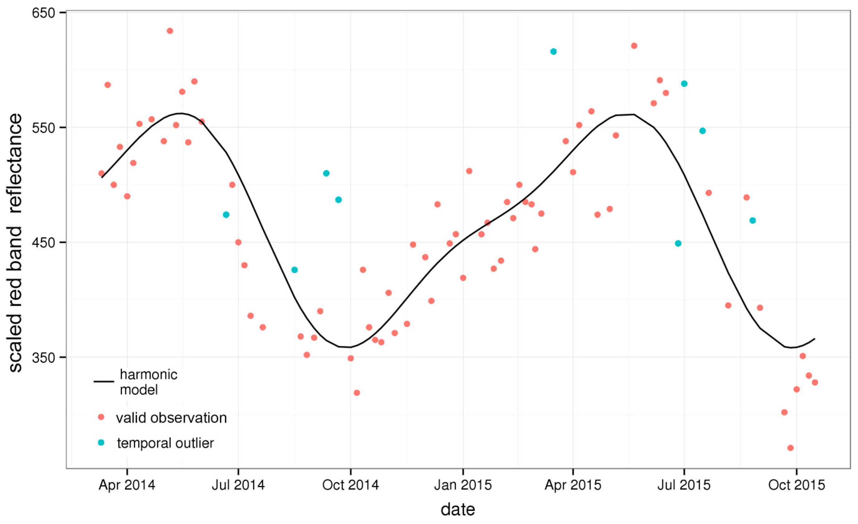
2.3. Temporal Cloud Filter

Remaining clouds in the RS time series can impair the extraction of seasonal information. In addition to cloud masking based on radiometry, sun-sensor geometry, and spatial-context, outliers in RS time series can be reduced by considering the temporal context with filters [22] or iterative outlier detection techniques [6,7,22]. We applied a smoothing based approach, by fitting a LOcally wEighted regreSsion Smoother (LOESS, [23,24]) to the time series per band and pixel. The Loess smoother, is a flexible approach that uses spline functions which enable the modelling and fitting of a wide variety of time series [25]. Observations were masked as clouds or cloud shadow where the difference between the observed data and the LOESS model exceeded a threshold. These thresholds and the parameters of the LOESS model were chosen based on expert knowledge and visual comparison of the results (details are provided in Appendix A,

Table A1. Parameters of the LOESS cloud detection. Thresholds are scaled top-of-atmosphere reflectance.

Band	Lower Threshold	Upper Threshold	LOESS Span
Blue	−80	-	0.3
SWIR	−120	120	0.3

). For the use cases, we chose the NIR and blue band to apply the cloud filter, since here clouds and cloud-shadows show up most clearly. The quality of the cloud detection was assessed using 100 randomly selected points marked as clear in the product cloud mask. 30% of the sample points were selected from the new cloud detected areas, while 70% were selected from clear areas. The points were visually interpreted as cloud or clear.

2.4. Time Series Metrics

Several methods have been applied to derive phenological information from RS time series. In the most simple approaches, time is just treated as an identifier and multiple observations are directly used as input features of the classification, or statistical metrics are derived for the different intervals of the time series [1,26,27]. An additional step is the fitting of models to the time series and using either the model parameters for classification directly [28], or deriving statistical metrics and phenological parameters such as start- and end of season from the models [11,22,29]. Other methods compare and cluster time series patterns using similarity measures, e.g., Euclidian distances, Fourier based similarities [20,30], or dynamic time warping [30,31]. Similar to [28], we used seasonal model parameters as metrics and descriptive statistics. Per band and pixel i, we derived median and percentiles and fitted a linear harmonic model to the time series as described in Equation (1), where x is the Julian day and T is the number of days per year (365/366):

$$\widehat{\rho }\left(i, x\right)= a_{1,i}+ b_{1,i}\cos \left(\frac{2\pi }{T}x\right)+ c_{1,i}\sin \left(\frac{2\pi }{T}x\right)+ b_{2,i}\cos \left(\frac{4\pi }{T}x\right)+ c_{2,i}\sin \left(\frac{4\pi }{T}x\right).$$

(1)

The coefficients of this model were then used as metrics for overall level (a_1,i) and seasonality (b_1,i, c_1,i, c_2,i, and b_2,i). Figure 2 shows an example time series of red reflectance with the fitted harmonic model. Additionally, for each spectral band the 10, 50, and 90 percent quantiles over the complete time series were derived as descriptive metrics. The coefficients of the model together with the quantiles derived per pixel time series were used as predictor variables in the RF classifier (see Section 2.5).

2.5. Classifier

A wide range of algorithms are used as classifiers in LC mapping [32]. For the use cases, we applied the RF algorithm since it has relatively simple parameterization, computation efficiency, and high accuracy [21,33], and has been used successfully to derive LC from seasonal models of RS time series [28]. The random forest classifier is based on a machine learning algorithm which constructs many decision tree classifiers based on bootstrapped samples [33]. Several advantages of the random forest method over other classifiers have been reported in the literature, including the ability to accommodate many predictor variables, as well as the fact that it is a non-parametric classifier which does not assume any underlying distribution in the training samples [33]. Random forest classifications generally assign class labels based on the majority vote among all bootstrapped classification trees. We used the ranger [34] package, an implementation in R and C++ of the original algorithm described in [33] which allows efficient parallel execution. The time series metrics (Section 2.4) are used as predictor variables within the RF model to predict and derive the LC.

2.6. Implementation

With the aim of making the analysis scalable and reproducible, we implemented our method with open source software (notably R [35], Linux, GDAL, Python) on the ESA Cloud Toolbox infrastructure [36], made available and operated by ESA Research and Service Support [14]. This scalable storage and computing environment (RAM and CPU can be tuned according to the user needs) allowed high performance computing. The Cloud Toolbox made it possible to cover the relatively large study area in only a few days of processing.

3. Results

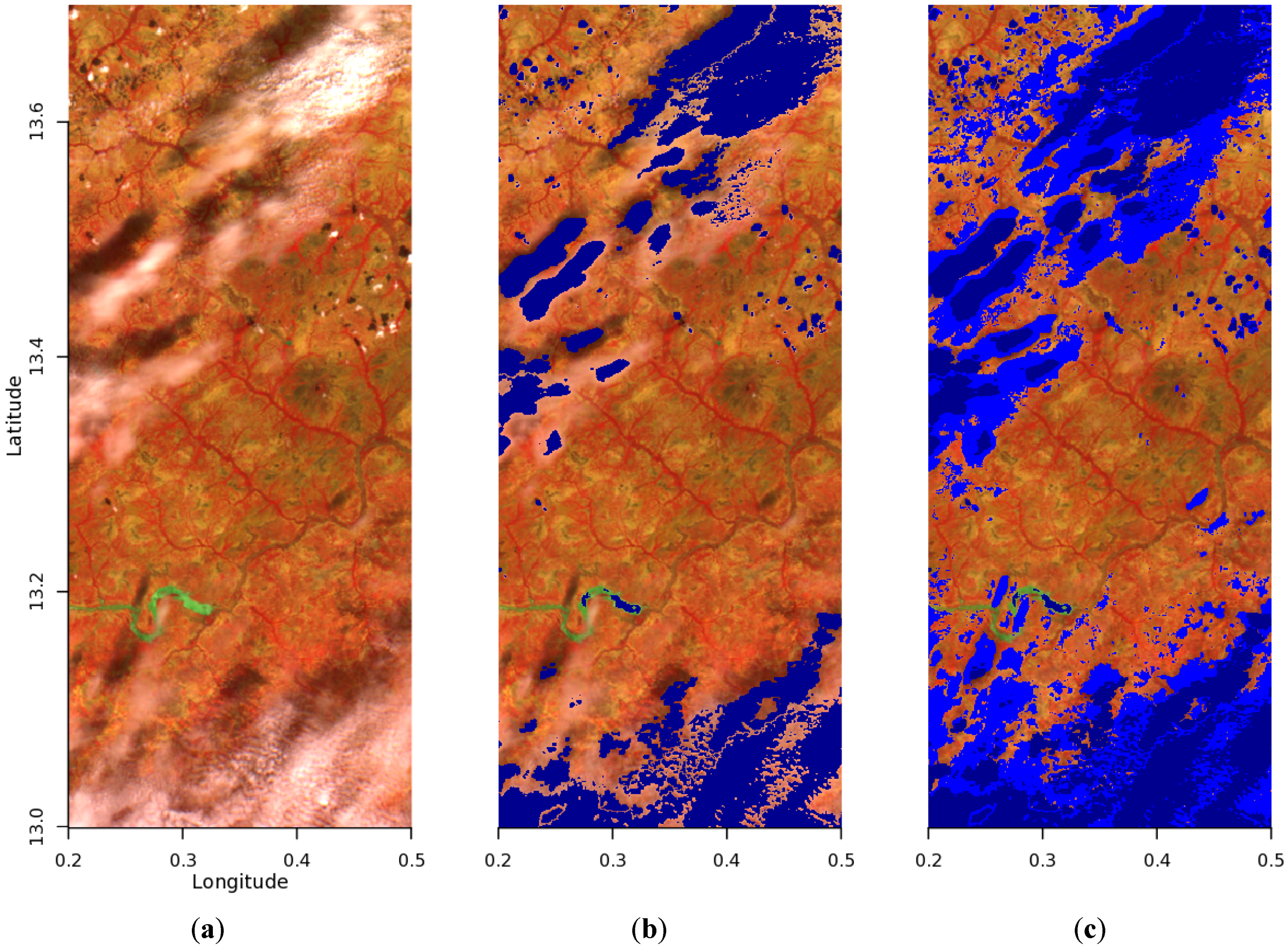
3.1. Temporal Cloud Filter and Metrics

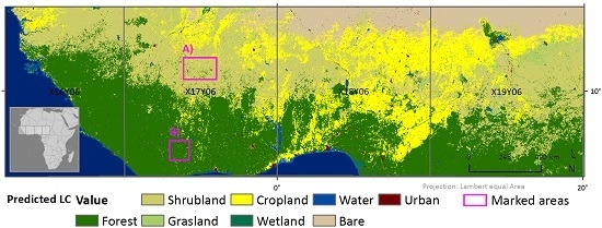
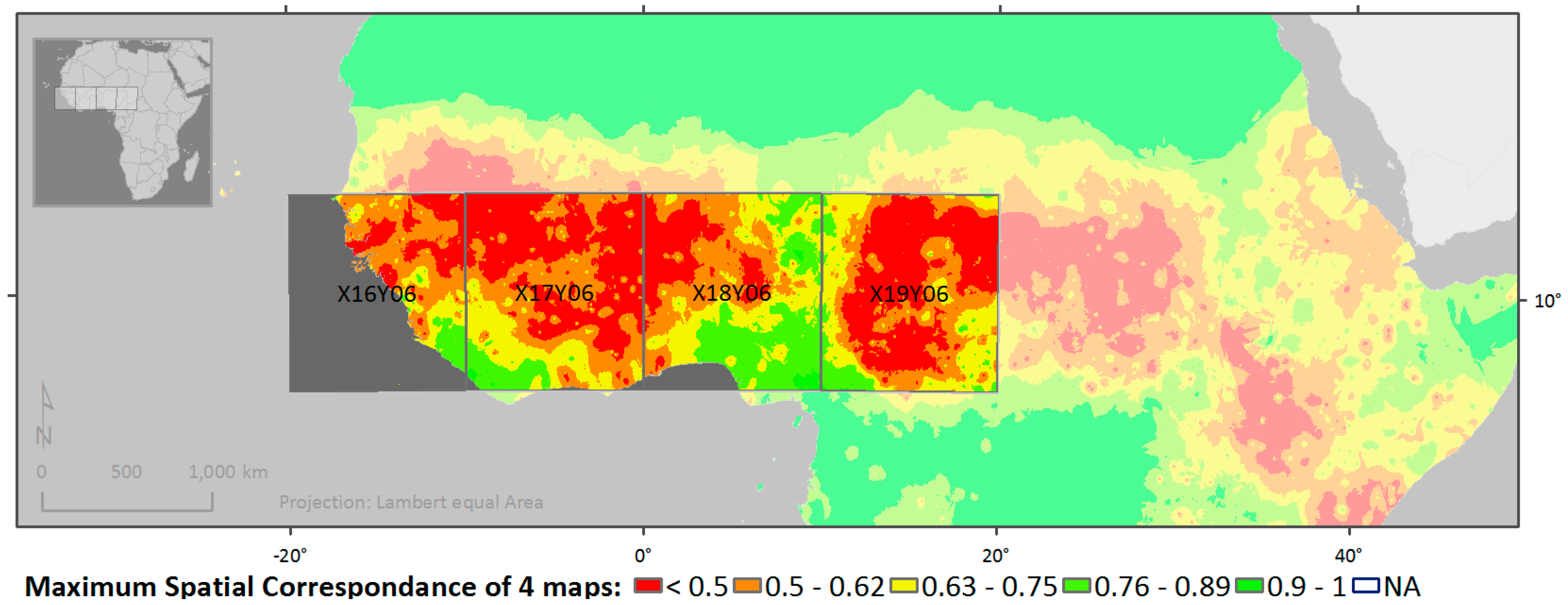
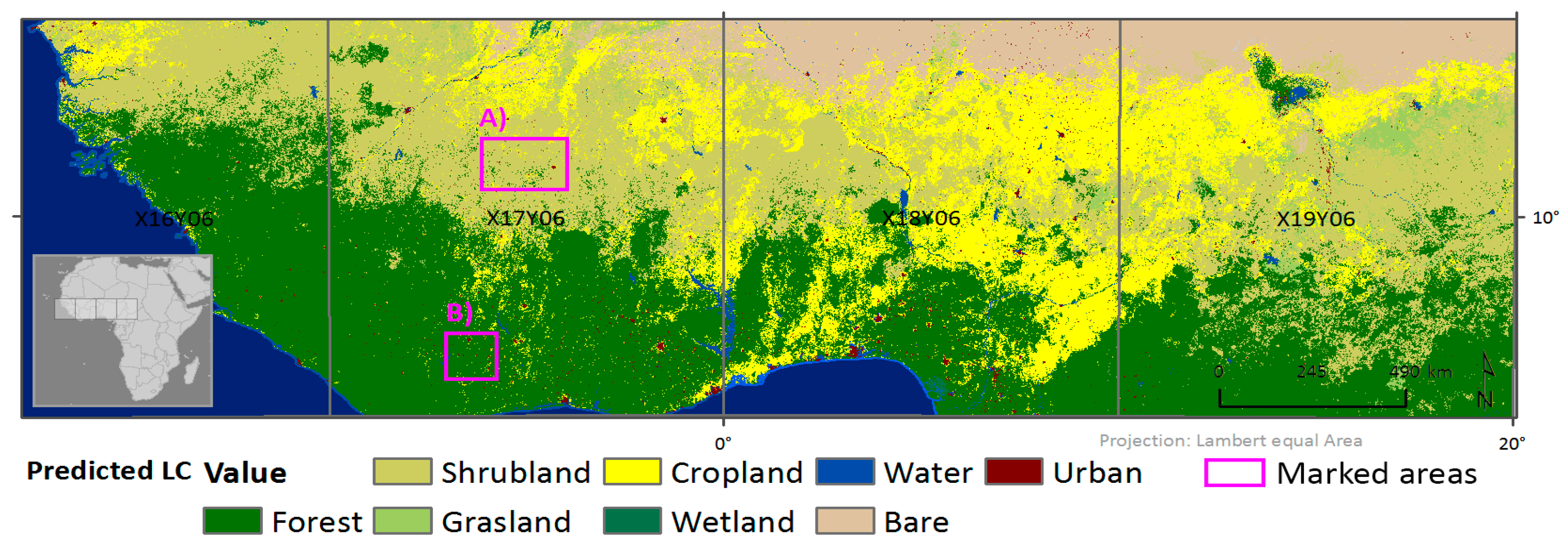
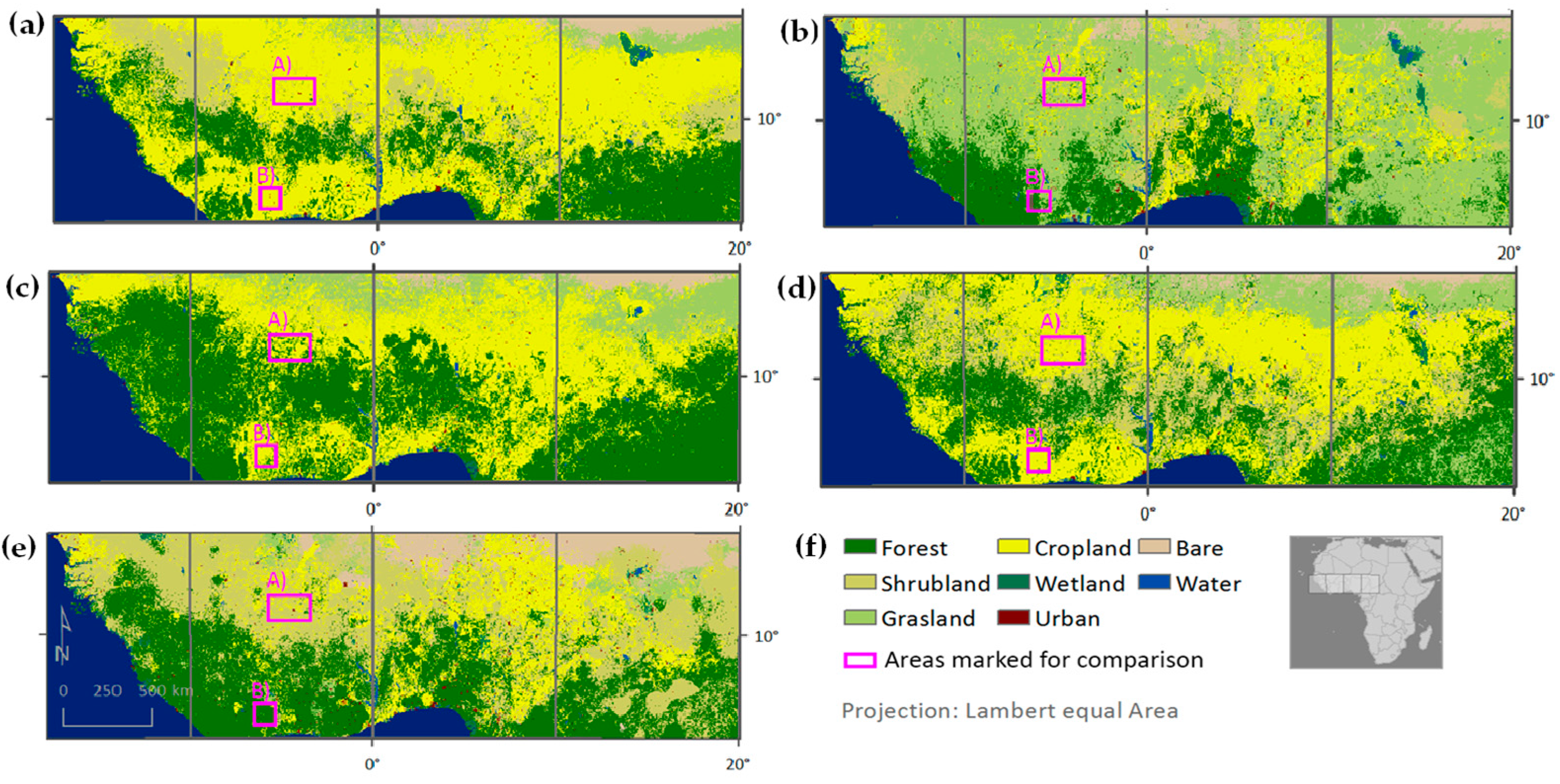
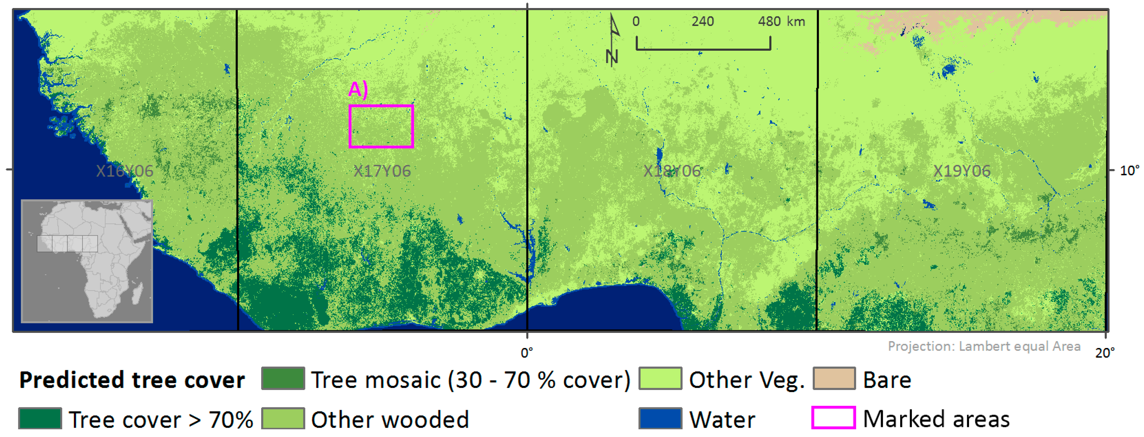
The temporal cloud filter detected semi-transparent and small clouds successfully. Figure 3 shows a comparison of the unfiltered data, the product cloud filter from the product SM mask, and the temporal cloud filter for a single observation and subset of the data.

A comparison of 100 reference points and the time series based cloud detection (see Section 2.3) showed 89 percent correspondence. It should be noted that the commission of cloud free observations was not always clearly distinguishable visually.

3.2. Use Cases

For the LC use case, the overall accuracy was 0.68. Commission and omission error per class are listed in

Table 1. Omission and commission error per class for the LC use case (out of bag (OOB) cross validation).

Error	Forest	Shrubland	Grassland	Cropland	Bare
Omission	0.290	0.401	0.175	0.302	0.487
Commission	0.223	0.404	0.252	0.366	0.412

. Note that these are based on OOB cross validation and are not a representative sample of the mapping area. While forest, grassland, and cropland were classified reasonably well, the shrubland and bare classes show higher errors.

A comparison of the existing LC global datasets for the study area with our map shows great difference in the classification of grassland, shrubland, and cropland, visible when comparing Figure 4 to Figure 5. Our classification is most similar to the integrated map from [5]. For example, the box marked with A) in the figures indicates an area classified predominantly as shrubland in our classification and the integrated map from [5], while it is mostly cropland in the LC-CCI and Globcover-2009 maps, grassland in the Globeland30 map, and cropland and forest in the MODIS map.

Of the global datasets, the MODIS 2010 shows the highest correspondence to our classification and the integrated map (

Table 2. Comparison of the overall accuracies of (1) our LC use case; (2) global LC maps; and (3) the regression kriging integrated map [5] compared to the integrated reference dataset.

Overall Accuracy	(1) LC Use Case	(2) Land Cover-CCI	Globeland30	MODIS 2010	Gobcover-2009	(3) Integrated Map
For study area 1	0.68	0.51	0.55	0.61	0.47	-
For Africa 2	-	0.55	0.57	0.63	0.51	0.76

¹ Water, urban, and snow/ice classes omitted. ² As derived in [5].

). Interestingly, similar to our map, the MODIS product relies heavily on dense satellite time series [27]. However, the MODIS map shows more cropland in the lower latitudes; an example is the area marked with box B). These areas are also classified as cropland in the LC-CCI and Globland-2009 maps, but as forest in our classification and the integrated map, while Globeland30 shows grassland for this area, which is generally more dominant in this map.

Figure 6 depicts the results of the FC use case. Visual comparison between the results of the use cases show that most of the shrubland and large parts of the forest class of the LC map is mapped as other wooded land in the FC use case; for example, the area marked with box A). The bare area in the FC case was much smaller, and most cropland and bare area of the LC case was other vegetation in the FC map.

Validation against the TREES-3 reference sample resulted in a good overall accuracy (0.899) and low omission and commission errors for almost all classes, the highest value being the commission error of the tree mosaic class (0.344), see

Table 3. Omission and commission error per class for the FC use case (validation sample).

	Tree Cover (70%)	Tree Mosaic	Other Wooded Land	Other Vegetation	Water
Omission error	0.164	0.245	0.164	0.098	0.130
Commission error	0.181	0.344	0.117	0.114	0.218

.

The variable importance measures of the RF models indicate that for both use cases, the intercept, 90% quantiles, and first seasonal coefficient of the NDVI time series model contributed most to the classification, followed by SWIR 90% quantiles (results not shown).

4. Discussion and Conclusions

PROBA-V data proofs are suited for large scale LC analysis, with its dense image time series at a finer spatial resolution (100 m) than common medium-resolution products (e.g., MODIS, SPOT-VEGETATION), and lighter data handling and processing compared to Landsat-like products. The high importance of variables, namely the seasonal metrics, supports our assumption that with the temporal density of the PROBA-V product, reconstruction of seasonal patterns in the tropics is possible despite high cloud contamination.

Even though the parameters of the temporal cloud filter were calibrated manually, it performs well in comparison with the existing product cloud detection. For larger scale application, a training dataset could be used to optimize the parameters of the cloud filter.

The presented filtering approach could potentially improve the commission of bright desert areas as cloud compared to the current PROBA-V preprocessing (November 2015), since we applied thresholds in a spatial-temporal context rather than absolute values. This is similar to the announced upcoming update of the PROBA-V product cloud detection based on global albedo data [15], but does not require auxiliary datasets. Our approach is less suited to distinguish ice clouds from snow/ice, which is not relevant over our study area but problematic in the current PROBA-V preprocessing chain [15].

The mediocre validation results of the LC use case should be seen in the context of the accuracies of common global LC maps for the study area. As visible in Figure 1, the maximum spatial correspondence of the global maps for the study area was below 0.5 for large areas. Our approach and the integration approach in [5] seem to deal better with difficult LC mapping conditions (e.g., heterogeneous landscapes) of the semi-arid ecosystems. However, it must be noted that for the global LC maps the reference data is truly independent, while for our map and the integrated map the reference data was also used for training. More reference data would be needed to compare the approaches under the same conditions.

The results from the FC use case demonstrate that our approach with PROBA-V time series is well suited to reproduce a product based on Landsat at a coarser spatial resolution. This is remarkable; we expected a higher mismatch due to the missing spatial detail and spectral bands. The differences between the use cases can largely be attributed to the different class definitions; for example, the forest class of the LC use case includes areas with tree cover above 15 percent.

Both classification use cases are limited in their thematic detail with rather few classes since they are intended mostly for demonstrative purpose based on existing datasets. Therefore, specific landscapes present in the Sahel such as banded vegetation patterning [37], different tree species, or crop types were not considered in this study, although accurate classification of these specific LC types could be possible with the methods described in this study if sufficient reference data is available. Alternatively, a classification of the proportions of main LC types (e.g., percent tree cover or percent shrub cover) [38] instead of categorical classes could be used to better characterize the heterogeneous landscapes in the Sahel.

Intra-annual variation in the spectral reflectance can help to further improve the classification results [1] when a longer record of PROBA-V data is available. This can be integrated in our approach by adding metrics that capture inter-annual trends. PROBA-V data could also be integrated with other long term time series data such as MODIS and SPOT-VGT to better capture intra-annual variability. Atzberger et al. [39] have evaluated the potential unmixing approaches to facilitate long spectral time series of SPOT-VGT and PROBA-V data. Further research is needed to fully exploit the potential of long consistent time series data to improve land cover classification in highly dynamic semi-arid ecosystems. The PROBA-V record then becomes very interesting for large-scale time series based change detection, as presented in [28,40]. Since the integration of existing LC maps also improves the accuracy, a hybrid approach using both existing datasets and PROBA-V time series data should be followed up.

Our modular implementation is geared towards a flexible classification platform. As demonstrated in the use cases, it can be adapted to different thematic applications. The users can select which metrics to compute and plug-in their sets of training data and different classifiers or machine learning algorithms. This can be developed into a cloud-based service, lifting the burden of big-data processing from the users. This would allow them to develop and test new time series based methods and applications quickly, and deploy them on large areas.

This paper illustrates a proof of concept for cloud-based “big-data” driven LC monitoring by implementing machine learning techniques in combination with in-situ training data sets to optimize LC monitoring in semi-arid ecosystems. The advent of cloud-based platforms (e.g., PROBA-V mission exploitation platform, Google Earth Engine), will not only revolutionize the way we deal with satellite data, but also enable the capacity to create multiple LC maps for different end-users using various training sets as input. We have shown that detailed temporal metrics can be extracted from PROBA-V 100 m image time series to continuously optimize global LC monitoring. Time series based LC monitoring approaches at 100 m resolution offer clear advantages in challenging semi-arid areas.

References

1. Hüttich, C.; Herold, M.; Wegmann, M.; Cord, A.; Strohbach, B.; Schmullius, C.; Dech, S. Assessing effects of temporal compositing and varying observation periods for large-area land-cover mapping in semi-arid ecosystems: Implications for global monitoring. Remote Sens. Environ. 2011, 115, 2445–2459. [Google Scholar] [CrossRef]
2. Sankaran, M.; Hanan, N.P.; Scholes, R.J.; Ratnam, J.; Augustine, D.J.; Cade, B.S.; Gignoux, J.; Higgins, S.I.; Le Roux, X.; Ludwig, F. Determinants of woody cover in African savannas. Nature 2005, 438, 846–849. [Google Scholar] [CrossRef] [PubMed]
3. Herold, M.; Mayaux, P.; Woodcock, C.; Baccini, A.; Schmullius, C. Some challenges in global land cover mapping: An assessment of agreement and accuracy in existing 1 km datasets. Remote Sens. Environ. 2008, 112, 2538–2556. [Google Scholar] [CrossRef]
4. Jung, M.; Henkel, K.; Herold, M.; Churkina, G. Exploiting synergies of global land cover products for carbon cycle modeling. Remote Sens. Environ. 2006, 101, 534–553. [Google Scholar] [CrossRef]
5. Tsendbazar, N.-E.; de Bruin, S.; Fritz, S.; Herold, M. Spatial accuracy assessment and integration of global land cover datasets. Remote Sens. 2015, 7, 15804–15821. [Google Scholar] [CrossRef]
6. Zhu, Z.; Woodcock, C.E. Automated cloud, cloud shadow, and snow detection in multitemporal Landsat data: An algorithm designed specifically for monitoring land cover change. Remote Sens. Environ. 2014, 152, 217–234. [Google Scholar] [CrossRef]
7. Goodwin, N.R.; Collett, L.J.; Denham, R.J.; Flood, N.; Tindall, D. Cloud and cloud shadow screening across Queensland, Australia: An automated method for Landsat TM/ETM+ time series. Remote Sens. Environ. 2013, 134, 50–65. [Google Scholar] [CrossRef]
8. Herold, M. An Assessment of National Forest Monitoring Capabilities in Tropical Non-Annex I Countries: Recommendations for Capacity Building; GOFC-GOLD Land Cover Project Office: Wageningen, The Netherlands; Friedrich Schiller University Jena: Jena, Germany, 2009. [Google Scholar]
9. Hansen, M.C.; Potapov, P.V.; Moore, R.; Hancher, M.; Turubanova, S.; Tyukavina, A.; Thau, D.; Stehman, S.; Goetz, S.; Loveland, T. High-resolution global maps of 21st-century forest cover change. Science 2013, 342, 850–853. [Google Scholar] [CrossRef] [PubMed]
10. Dierckx, W.; Sterckx, S.; Benhadj, I.; Livens, S.; Duhoux, G.; Van Achteren, T.; Francois, M.; Mellab, K.; Saint, G. PROBA-V mission for global vegetation monitoring: Standard products and image quality. Int. J. Remote Sens. 2014, 35, 2589–2614. [Google Scholar] [CrossRef]
11. Lambert, M.-J.; Waldner, F.; Defourny, P. Cropland mapping over sahelian and sudanian agrosystems: A knowledge-based approach using PROBA-V time series at 100-m. Remote Sens. 2016, 8, 232. [Google Scholar] [CrossRef]
12. Roumenina, E.; Atzberger, C.; Vassilev, V.; Dimitrov, P.; Kamenova, I.; Banov, M.; Filchev, L.; Jelev, G. Single-and multi-date crop identification using PROBA-V 100 and 300 m S1 products on Zlatia test site, Bulgaria. Remote Sens. 2015, 7, 13843–13862. [Google Scholar] [CrossRef]
13. Bodart, C.; Brink, A.B.; Donnay, F.; Lupi, A.; Mayaux, P.; Achard, F. Continental estimates of forest cover and forest cover changes in the dry ecosystems of Africa between 1990 and 2000. J. Biogeogr. 2013, 40, 1036–1047. [Google Scholar] [CrossRef] [PubMed]
14. Marchetti, P.; Rivolta, G.; D’Elia, S.; Farres, J.; Gobron, N.; Mason, G. A model for the scientific exploitation of Earth Observation missions: The ESA research and service support. In IEEE Geoscience and Remote Sensing Society Newsletter; No. 162; IEEE: New York, NY, USA, 2012; pp. 10–18. [Google Scholar]
15. Wolters, E.; Swinnen, E.; Dierckx, W. Improved PROBA-V cloud detection using globalbedo surface albedo data 2016. In Proceedings of the PROBA-V Symposium, Gent, Belgium, 26–28 January 2016.
16. VITO. Product Distribution Portal. Available online: http://www.vito-eodata.be (accessed on 5 March 2015).
17. GOFC-GOLD. GOFC-Gold Reference Data Portal. Available online: https://bm-wageningen.cartodb.com/viz/efcf03a8-15de-11e5-86c4-0e4fddd5de28/embed_map (accessed on 1 October 2015).
18. Fritz, S.; McCallum, I.; Schill, C.; Perger, C.; See, L.; Schepaschenko, D.; Van der Velde, M.; Kraxner, F.; Obersteiner, M. Geo-Wiki: An online platform for improving global land cover. Environ. Model. Softw. 2012, 31, 110–123. [Google Scholar] [CrossRef]
19. Tsendbazar, N.-E.; de Bruin, S.; Herold, M. Integrating global land cover datasets for deriving user-specific maps. Int. J. Digit. Earth 2016, in press. [Google Scholar] [CrossRef]
20. Abade, N.A.; Júnior, O.A.d.C.; Guimarães, R.F.; de Oliveira, S.N. Comparative analysis of MODIS time-series classification using support vector machines and methods based upon distance and similarity measures in the Brazilian Cerrado-Caatinga boundary. Remote Sens. 2015, 7, 12160–12191. [Google Scholar] [CrossRef]
21. Rodriguez-Galiano, V.F.; Ghimire, B.; Rogan, J.; Chica-Olmo, M.; Rigol-Sanchez, J.P. An assessment of the effectiveness of a random forest classifier for land-cover classification. ISPRS J. Photogramm. Remote Sens. 2012, 67, 93–104. [Google Scholar] [CrossRef]
22. Hamunyela, E.; Verbesselt, J.; Roerink, G.; Herold, M. Trends in spring phenology of western European deciduous forests. Remote Sens. 2013, 5, 6159–6179. [Google Scholar] [CrossRef]
23. Cleveland, W.S.; Grosse, E.; Shyu, W.M. Local regression models. In Statistical Models in S; Chapter 2; Taylor & Francis: Abingdon, UK, 1992; pp. 309–376. [Google Scholar]
24. Cleveland, R.B.; Cleveland, W.S.; McRae, J.E.; Terpenning, I. STl: A seasonal-trend decomposition procedure based on loess. J. Off. Stat. 1990, 6, 3–73. [Google Scholar]
25. Verbesselt, J.; Hyndman, R.; Newnham, G.; Culvenor, D. Detecting trend and seasonal changes in satellite image time series. Remote Sens. Environ. 2010, 114, 106–115. [Google Scholar] [CrossRef]
26. Friedl, M.A.; McIver, D.K.; Hodges, J.C.; Zhang, X.; Muchoney, D.; Strahler, A.H.; Woodcock, C.E.; Gopal, S.; Schneider, A.; Cooper, A. Global land cover mapping from MODIS: Algorithms and early results. Remote Sens. Environ. 2002, 83, 287–302. [Google Scholar] [CrossRef]
27. Friedl, M.A.; Sulla-Menashe, D.; Tan, B.; Schneider, A.; Ramankutty, N.; Sibley, A.; Huang, X. MODIS collection 5 global land cover: Algorithm refinements and characterization of new datasets. Remote Sens. Environ. 2010, 114, 168–182. [Google Scholar] [CrossRef]
28. Zhu, Z.; Woodcock, C.E. Continuous change detection and classification of land cover using all available landsat data. Remote Sens. Environ. 2014, 144, 152–171. [Google Scholar] [CrossRef]
29. Melaas, E.K.; Friedl, M.A.; Zhu, Z. Detecting interannual variation in deciduous broadleaf forest phenology using Landsat TM/ETM+ data. Remote Sens. Environ. 2013, 132, 176–185. [Google Scholar] [CrossRef]
30. Lhermitte, S.; Verbesselt, J.; Verstraeten, W.W.; Coppin, P. A comparison of time series similarity measures for classification and change detection of ecosystem dynamics. Remote Sens. Environ. 2011, 115, 3129–3152. [Google Scholar] [CrossRef]
31. Petitjean, F.; Inglada, J.; Gançarski, P. Satellite image time series analysis under time warping. IEEE Trans. Geosci. Remote Sens. 2012, 50, 3081–3095. [Google Scholar] [CrossRef]
32. Lu, D.; Weng, Q. A survey of image classification methods and techniques for improving classification performance. Int. J. Remote Sens. 2007, 28, 823–870. [Google Scholar] [CrossRef]
33. Breiman, L. Random forests. Mach. Learn. 2001, 45, 5–32. [Google Scholar] [CrossRef]
34. Wright, M.N.; Ziegler, A. Ranger: A fast implementation of Random Forests for high dimensional data in C++ and R. arXiv Preprint 2015. [Google Scholar]
35. R Development Core Team. R: A Language and Environment for Statistical Computing; R Foundatation for Statistical Computing: Vienna, Austria, 2013. [Google Scholar]
36. European Sociological Association (ESA). RSS Cloud Service. Available online: http://wiki.services.eoportal.org/tiki-index.php?page=RSS+CloudToolbox+Service (accessed on 23 September 2015).
37. Deblauwe, V.; Barbier, N.; Couteron, P.; Lejeune, O.; Bogaert, J. The global biogeography of semi-arid periodic vegetation patterns. Glob. Ecol. Biogeogr. 2008, 17, 715–723. [Google Scholar] [CrossRef]
38. Walton, J.T. Subpixel urban land cover estimation. Photogramm. Eng. Remote Sens. 2008, 74, 1213–1222. [Google Scholar] [CrossRef]
39. Atzberger, C.; Formaggio, A.R.; Shimabukuro, Y.E.; Udelhoven, T.; Mattiuzzi, M.; Sanchez, G.A.; Arai, E. Obtaining crop-specific time profiles of NDVI: The use of unmixing approaches for serving the continuity between SPOT-VGT and PROBA-V time series. Int. J. Remote Sens. 2014, 35, 2615–2638. [Google Scholar] [CrossRef]
40. Verbesselt, J.; Zeileis, A.; Herold, M. Near real-time disturbance detection using satellite image time series. Remote Sens. Environ. 2012, 123, 98–108. [Google Scholar] [CrossRef]
Figure 1. Maximum spatial correspondence of four global land cover (LC) maps (Globcover-2009, Land Cover-CCI-2010, MODIS-2010, and Globeland30-2010) with independent reference data as derived in [5] and the extent of our study area over West Africa. Note that the maximum correspondence for large parts of the study area is below 50%.
Remotesensing 08 00987 g001
Figure 2. Example PROBA-V time series (red band scaled reflectance) with a fitted harmonic model (black line) as described in Equation (1), used to derive time series metrics.
Remotesensing 08 00987 g002
Figure 3. Comparison of false color composites of a subset of a PROBA-V image acquired on 11 October 2015. (a) unfiltered data; (b) the cloud mask of the product SM layer and (c) the product cloud mask (dark blue) extended by our cloud mask (lighter blue) based on temporal outliers.
Remotesensing 08 00987 g003
Figure 4. Result of the LC classification use case based on PROBA-V 100 m data. The urban and water areas are adapted from the LC-CCI 2010 map. Boxes A) and B) mark example areas with pronounced differences to the global LC maps depicted in Figure 5.
Remotesensing 08 00987 g004
Figure 5. Thematically harmonized LC maps for the study area: (a) Land Cover-CCI; (b) Globeland30, (c) MODIS 2010; (d) Gobcover-2009 and (e) regression kriging based integration of (ad) as presented in [5]; (f) Legend. Large differences between the classifications are visible, see, e.g., marked areas A) and B). For details of the thematic harmonization, see [5].
Remotesensing 08 00987 g005
Figure 6. Result of the forest cover (FC) classification use case.
Remotesensing 08 00987 g006