1. Introduction
Savannahs cover approximately 20% of the Earth’s land surface and are characterised as a grassland ecosystem, with trees being sufficiently widely spaced so that the canopy does not close [
1]. The understorey herbaceous layer consists primarily of grasses [
1] which are a major contributor to the carbon balance. To a large extent these areas are extensively grazed by native, domestic, and feral herbivores—supporting conservation, tourism, and pastoral activities [
2]. Pastures play an important role in rangeland ecology, ecosystem services, and livestock-related industries [
2]. Physical sampling of pasture biomass over large areas is not generally considered feasible in rangeland and savannah systems; it is not possible to collect and collate sufficient field data to adequately inform land managers and provide sufficient input for pasture biomass modelling [
3]. A major issue is the estimation of pasture biomass for livestock forage budgeting and conservation purposes [
4]. Spatially explicit seasonal pasture biomass estimates could assist land managers and a host of other stakeholders to make assessments relating to livestock production and land resource management.
Pasture biomass estimates from space have been actively pursued over time with varying approaches, initially relating vegetation cover to biomass [
5]. Vegetation indices of optical satellite imagery such as NDVI (Normalised Differenced Vegetation Index) or EVI (Enhanced Vegetation Index) focus on the green vegetation component. A general relationship between vegetative ground cover and pasture biomass exists for low ground cover areas, but when the ground cover is close to 100% the cover-to-mass relationship saturates and reliable estimates are not possible even at low biomass levels [
6,
7,
8]. Investigating this relationship, Hobbs [
5] related four vegetation indices to field data and found a breakdown of biomass levels >1000 kg/ha. The authors of [
9] had success in relating bulk-green pasture biomass to NDVI for their study site in New Zealand, but also found that pasture biomass estimates based on NDVI were saturating. This has been confirmed in other studies, for example, Kawamura et al. [
10], who compared NDVI and EVI from MODIS (Moderate Resolution Imaging Spectroradiometer) and AVHRR (Advanced Very High Resolution Radiometer) and found a saturation in the relationship when NDVI and EVI values were approximately 0.9 and 0.8, respectively. In most savannah systems this approach has significant limitations for pasture biomass estimation due to the presence of senescent dry grass and tree cover. To overcome this direct limitation e.g., Edirisinhe et al. [
7] and Holm [
11] used time series of optical MODIS and AVHRR imagery for a quantitative pasture biomass assessment using cumulative NDVI data. The author of [
12] has related MODIS BRDF parameters to pasture biomass, with some success. Other approaches rely on physically based models incorporating remotely sensed raster images and meteorological data to model and forecast pasture biomass [
4]. It is likely that cover-to-mass relationships are variable with pasture composition and the degree of grazing necessitating location specific calibration of satellite indices.
Synthetic Aperture Radar (SAR) imagery from active sensors can add to the cover signal as the backscatter data provide structural information of the surface [
13,
14]. In a review on biomass mapping with optical and SAR imagery, Kumar et al. [
15] include a section on grasslands and reported that very few studies so far are using SAR for pasture biomass estimation. SAR imagery is a two-dimensional representation of the surface backscatter from an active sensor [
16]. A range of SAR imaging systems exists in different wavelength, most notably: P-band (30–100 cm), L-band (15–30 cm), S-band (15–30 cm), C-band (3.75–7.5 cm), or X-band (2.4–3.75 cm). The sideways-looking radar pulses or chirps are emitted and recorded in either horizontal or vertical polarisation. The phase and backscatter information, converted to complex data, are stored in image bands with four potential polarisation combinations (quad-pol): HH, VV, VH, and HV (the first letter indicated the emitted and the second the received polarisation). The received backscatter from the surface is dependent on (a) sensor parameters, such as wavelength, polarisation, look angle, and resolution; and (b) scene parameters, such as surface roughness, local terrain, dielectric properties, target density, and distribution [
16]. The features of interest should be on the order of magnitude of the wavelength, e.g., for pasture monitoring P-Band imagery with a 60-cm wavelength may not interact with the grass plants directly, while with lower wavelength, such as X-band, interactions with the grass stems are more likely [
14]. Different scattering mechanisms occur when the emitted photons interact with the surface (direct single scattering, direct ground reflection, double bounce, etc.). In complex structures, such as tree crowns, multiple scattering (in the lower wavelength) and a change in polarisation are common [
16].
The authors of [
17] applied C-band RADARSAT-2 HH imagery in an explorative study to assess grassland spatial heterogeneity and concluded that it is possible to map pasture biomass with SAR imagery. The authors of [
18] mapped pasture types in Western Australia and found that C-band SAR data alone were not effective for pasture discrimination, but the combination with optical imagery showed more discriminative power than either dataset alone. The authors of [
19] used a time series of optical and RADARSAT-2 quad-pol imagery for grassland/crop differentiation with support vector machines and found that SAR imagery (via parameters from poliametric decomposition) resulted in better classification accuracies than optical imagery (0.98 compared to 0.81) for their study site in Brittany. The authors of [
20] have analysed a time series of X-band TerrarSAR-X (TSX) and COSMO-SkyMed imagery in combination with Landsat and Spot-4 optical data to monitor irrigated grasslands. They compared the in situ data of vegetation properties with satellite imagery and concluded that X-band data are sensitive to variations in moisture irrespective of the grass cover, though the potential for X-band data for monitoring grassland growth is very limited. Their study achieved better results when monitoring soil moisture variations with X-band imagery. The authors of [
21] explored dual-polarisation ALOS PALSAR and TSX imagery (HH, VV) in combination with Landsat imagery and extensive field data for pasture biomass estimation. Their results showed some promise relating TSX-derived alpha entropy [
21] to pasture biomass, but the statistical relationship with field data was inconclusive. The authors of [
14] have used multi-temporal HH-polarised imagery from C-band ENVISAT ASAR, L-band ALOS PALSAR, and X-band COSMO-SkyMed for pasture monitoring in southern Australia. SAR backscatter data were correlated with vegetation indices derived from optical MODIS, Landsat, and SPOT 5 imagery and report on the feasibility of pasture biomass estimation with SAR imagery, particularly with X and C- band data in the early growing season. The authors of [
22] performed a robust regression estimation of pasture biomass with TSX (HH, HV) in New Zealand, with a time series of imagery between February 2008 and April 2009 and associated field observations. Their model revealed a regression-based biomass model with a mean residual error of 317 kg/ha.
So far, to the knowledge of the authors, no reliable pasture biomass monitoring system in savannah ecosystems based on satellite imagery has been published.
In our approach we have focused on the question of whether satellite imagery can be used to establish a pasture biomass model; and if TSX X-band data with 3.1 cm wavelength have sufficient interaction with grass species to add to pasture biomass estimation in comparison with biophysical image products from optical imagery alone.
2. Materials and Methods
2.1. Field Data
On-ground estimates of pasture biomass can be acquired by destructive and non-destructive (e.g., visual) means. Destructive methods involve laborious cutting and drying of a large number of samples of a known metric such as a quadrat (e.g., 0.25 m
2), where the dried biomass values are scaled up to estimate a larger area [
23]. Purely visual estimates of pasture biomass and larger areas often have large errors and are generally variable between different operators. The BOTANAL methodology [
24] employed in this study enables multiple users to traverse large transect lines, where quadrats are visually estimated at given distances and calibration curves are applied to scale up to larger (e.g., field-scale areas). This results in more accurate and less subjective estimates. The estimates are calibrated to destructive measurements of dried grass to represent TSDM (Total Standing Dry Matter).
Appendix lists Australian pastoralism terminology used in the text.
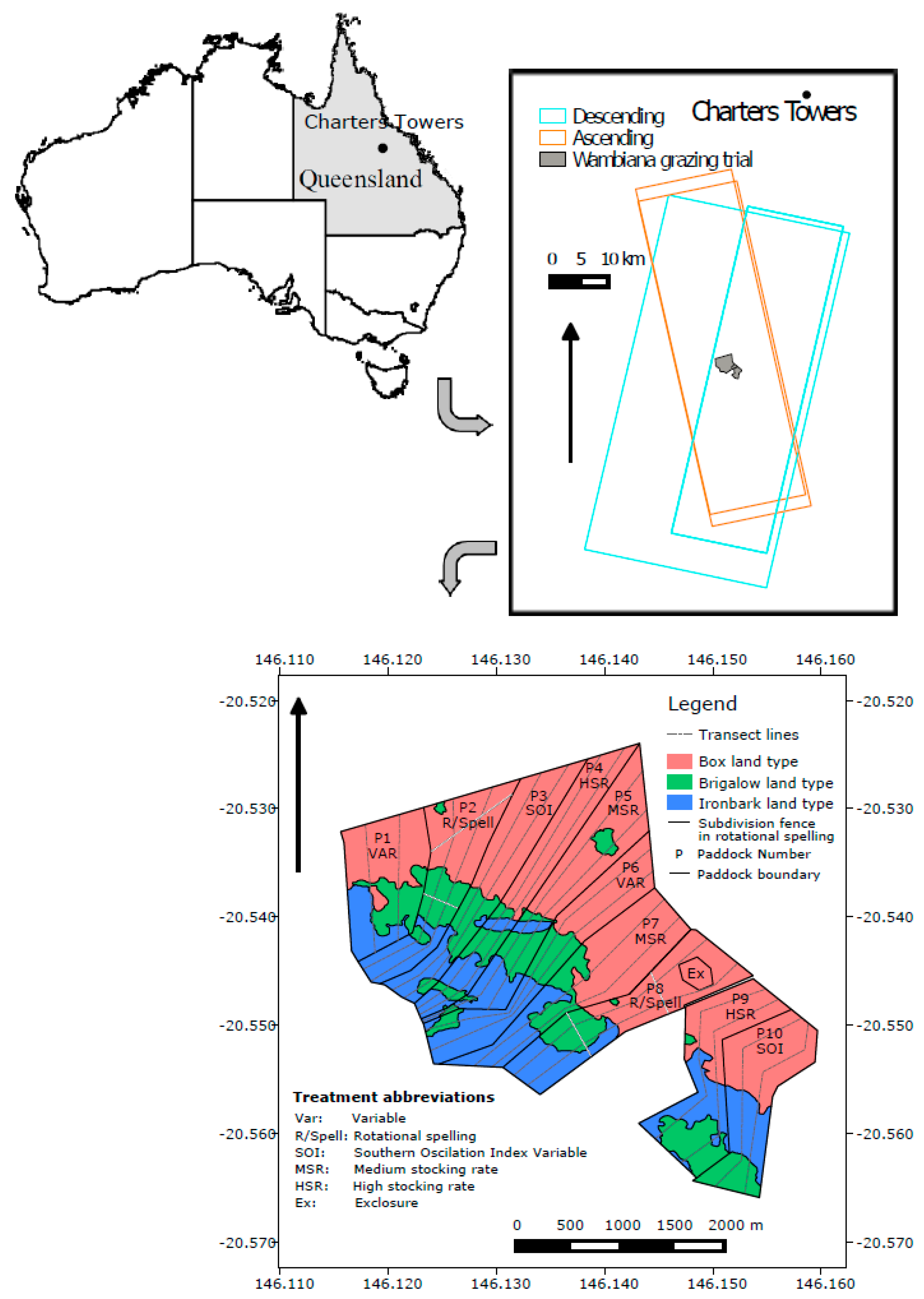
The Wambiana grazing trial site is located southwest of the township of Charters Towers in anopen woodland. The landscape of the trial is characterised by three main tree species of Reid River box (
Eucalyptus brownii), brigalow (
Acacia harpophylla), and silver leaf ironbark (
Eucalyptus melanophloia) (
Figure 1). Mature tree heights are typically 12–15 m, with a foliage projective cover [
25] ranging from 5%–20% across the paddock by land type combinations. The tree species are evergreen, but can suffer partial defoliation in drought, with the possibility of some variation in the canopy between the wet and dry seasons. Measure leaf size ranges for dominant tree species [
26,
27] are:
E. brownii (8–15 cm × 2–4 cm);
E. melanophloia (5–9 cm × 2–3 cm); and
A. harpophylla (10–20 cm × 0.7–1.6 cm), which are likely to interact with the 3.1 cm X-band wave lengths. An understorey of non-edible native shrubs (currant bush;
Carissa ovata) and false sandalwood (
Eremophila mitchellii) are present, with Carissa covering 25%–30% of the box land type [
28].
The dominant understorey native grasses include desert bluegrass (Bothriochloa ewartiana) and black speargrass (Heteropogon contortus), which are preferred for grazing; along with less desired grasses such as wiregrass (Aristida spp.) and wandarrie grass (Eriachne mucronata). These grasses are largely erect tussock grasses, generally less than 50 cm high with leaves less than 1 cm wide, although in recent years Indian couch (Bothriochloa pertusa), a more prostrate, thin-stemmed, introduced grass, has become increasingly present, particularly in heavily grazed treatments. The grasses generally change from green to dry as the season progresses and leaf disappears faster than stem material (with grazing and detachment). At higher stocking rates, grass tussocks at the end of the dry season are dominated by stem material (5–30 cm tall and 1–2 mm in diameter), generally from the least productive species. In prolonged drier periods (i.e., drought), there may be little standing material of any grass species present, with only grass crowns visible. The length-to-width ratio of the elements of the grass sward suggests that X-band radar should interact. Tussock density of the productive grasses can vary from about 5 tussocks/m2 to 1.5 tussocks/m2 in heavily grazed areas.
The soil types at the site are described as texture contrast (sodosols) associated with the Box trees, heavy clays (vertosols) aligned to the brigalow trees, and yellow-brown earths (kandosols) for the ironbark trees. The site is generally flat, with the heavy clay soils being “micro-gilgaied” (i.e., depressions) with vertical scales of a few centimetres.
The trial offers a time series of TSDM observations systematically and consistently acquired since 1997 to estimate land type and paddock scale TSDM. Five different grazing strategies with two replicates each have been tested on 10 paddocks, each 100 ha in size [
29], for assessing sustainable and profitable land management. The trial has clearly demonstrated the productive benefits of improved grazing management, in a manner and scale of direct relevance to the grazing industry of northern Australia. A key outcome of the trial is that a loss of land condition under heavy stocking compromised productivity, profitability, and the local environment [
28]. TSDM field data are acquired for the grazing trial at paddock scale in May and October each year. Two parallel transects per paddock were established, with vegetation and soil parameters recorded by experienced field operators approximately every 50 m along these transects (
Figure 1). TSDM estimates were made using calibrated visual observations (BOTANAL method) [
24], in association with 0.5 m × 0.5 m quadrats used to harvest pasture TSDM.
The Wambiana paddock grazing treatments and approximate stocking rates with 1 AE = 1 animal equivalent or 450 kg steer (only steers are used in the trial) are:
Medium stocking rate—relatively constant stocking at 8–10 ha/AE.
Heavy stocking rate—relatively constant stocking at 4–5 ha/AE to May 2005; thereafter stocked at 6 ha/AE until May 2009, when stocking rates were returned to 4 ha/AE.
Variable stocking—stocking rates adjusted upwards or downwards in May based on end of wet season feed availability (3–12 ha/AE).
SOI (Southern Oscillation Index) variable stocking—stocking rates adjusted upwards or downwards in October based on feed availability and SOI forecasts for the next wet season (3–12 ha/AE).
Rotational wet season spelling—spell a third of the paddock each wet season; relatively constant stocking at 7–8 ha/AE until November 2003 and at 8–10 ha/AE thereafter.
Pasture growth is strongly influenced by rainfall. The average long-term annual rainfall for the nearest climate station (17 km northwest of the site) is 643 mm, but annual rainfall is highly variable ranging from 207 to 1409 mm. The seasons related to this study were below average and are discussed in further detail below.
2.2. Optical Satellite Imagery and Products
Landsat data originating from the United States Geological Survey were utilised in this study. All available imagery for October/November 2014 and May/June 2015 were included (
Table 1). The Landsat imagery were atmospherically corrected, and cloud-masked following the standardised pre-processing steps, as described in [
30].
Biophysically meaningful standardized data products were used here:
(a) Foliage Projective Cover (FPC)
Foliage projective cover is a metric describing the vertical projection of the foliated tree canopy in units of percent [
25]. FPC is an important variable as the study site is located in anopen woodland, and thus are reflectance or backscatter signals influenced by the tree canopy. The authors of [
31] have developed a state-wide FPC data product based on dry-season Landsat imagery at 30 m pixel size. This product is based on a multiple regression of Landsat imagery with field observation of stand basal area (RMSE < 10%), validated with independent FPC estimates from LiDAR aerial survey (RMSE 5.3%) across the major vegetation communities in Queensland.
FPC predictions from all available Landsat 7 ETM+ and Landsat 8 OLI imagery within the period of October to November 2014 and May to June 2015 were accessed (
Table 2).
(b) Fractional Vegetation Cover (FVG)
Vegetative ground cover is a key piece of information in natural resource management and important for pasture biomass estimation [
32]. A 30-m Landsat Fractional Vegetation Cover dataset (FVC) was developed by [
33]. The data product contains fractional cover estimates of green vegetation, non-green vegetation, and bare ground summing to 100 percent plus model error. The authors incorporated 968 fractional vegetation cover field data points, collected at one hectare field sites [
23] across the states of Queensland and New South Wales (Australia) with the closest Landsat image observation (no more than 60 days apart). These data were used to derive image-based endmember spectra of green vegetation, non-green vegetation, and bare soil, which were applied in a spectral unmixing to generate Landsat-based predictions for these fractions with an RMSE of 11.8%.
All available single-date Landsat 8 images within the time interval of October to November 2014 and April to May 2015 were processed to FVC cover (
Table 1). The non-green vegetation component in the FVC product is a combined estimate of the senescent (non-green) vegetation and litter component, which will now be herein referred to as “dry vegetation”.
2.3. X-Band SAR Imagery: TerrarSar-X (TSX)
Imagery from the TSX instrument in StripMap mode were acquired for the end of the dry season (October/November) 2014 and the end of the wet season (May) 2015 (
Figure 1) with a 3.1 cm wavelength. Three overpasses in the dry season of 2014 (two with dual polarisation: HH/HV) and two dual-polarisation images (HH/HV) in the wet season of 2015 were obtained.
Table 2 lists the most relevant metadata of the images used.
The level 1b enhanced ellipsoid corrected imagery were calibrated and processed to terrain corrected γ
0 in decibels with the science toolbox exploitation platform (SNAP) provided by the European Space Agency [
34], following:
where
DN is the digital number,
k is the calibration coefficient, and
θloc is the local incidence angle.
2.4. Ancillary Data
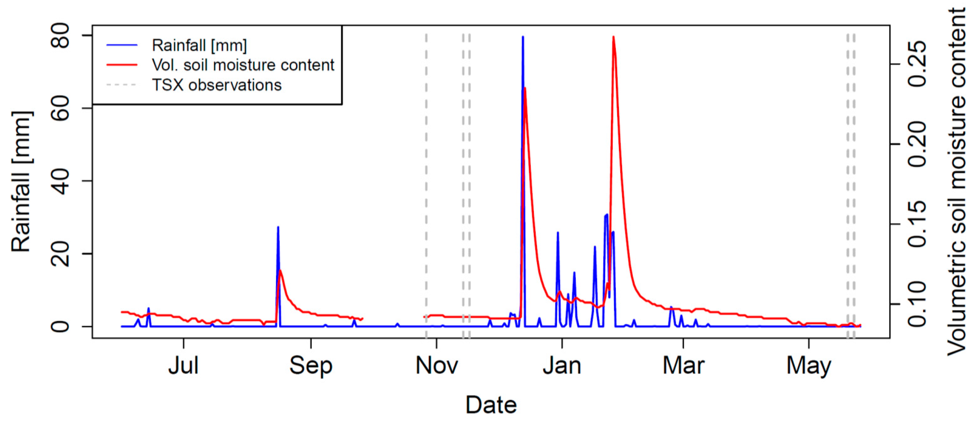
Daily rainfall data were extracted from the “Data Drill” option of the SILO climate database (Scientific Information for Land Owners; [
35]), which contains daily interpolated surfaces from available climate station data. The rainfall total of the displayed time interval (
Figure 2) of the dry season 2014 and the wet season 2015 was 369.6 mm, which was well below the long-term average (643 mm). Soil volumetric water data were recorded with a data logger located in Paddock 8 with a time domain reflectometry probe (TDR).
The wet season rainfall for the site was uncharacteristically low, coinciding with a strong El Niño event, which has a strong link with rainfall and vegetation growth in northeast Queensland [
36]. The soil surface was quite dry for all image acquisitions and slightly drier in the May 2015 data acquisitions. The average maximum day and minimum night air temperatures were 41.1 °C and 14.1 °C during the TSX observation period October 2014; and 32.4 °C and 11.0 °C in May 2015.
The vapour pressure deficit (VPD) was calculated from the SILO vapour pressure data following [
37]. VPD is the difference (deficit) between the amount of moisture in the air and how much moisture the air can hold when it is saturated. VPD was calculated as the evaporative power of the atmosphere in the boundary layer above the canopy and has been shown to be correlated with overstorey FPC [
25,
31].
2.5. Spatial Data Analysis
The TSDM transect data were spatially averaged by paddock-and-land type parcels, resulting in 37 observations for October 2014 and 37 observations for May 2015. The parcel averages may not have represented the barest areas, which had consistently low TSDM; therefore, four additional polygons were digitised from high-resolution imagery for areas with low TSDM and included as additional data. These low-TSDM areas had FPC values ranging from 0% to 18%.
To ensure a sample from a high-TSDM region was represented, a visual field estimate of TSDM was made from an area exclosed from grazing, located in Paddock 8. The parcels formed the basis for all further analysis. All available raster data were spatially averaged to match these units (
Figure 1).
The available single-date TSX data were used as well as temporal aggregations for a noise reduction: rasters of temporal minimum, maximum, and mean were calculated for the TSX HH and HV time series in 2014 and 2015, respectively. Mean rasters were calculated for the FPC and FVC data for the observation time intervals.
The Eureqa package [
38] was used to conduct an extensive search for linear and nonlinear functions using a large set of predictor variables. A robust multiple regression analysis was performed in the R package [
39] with the most prominent candidate variables: the single date and temporally aggregated datasets with the aim to generate TSDM maps for the two seasons in 2014 and 2015. The adjusted r
2 was used in reporting instead of the multiple r
2, as it adjusts for the number of terms in a model (i.e., it decreases when a predictor improves the model by less than expected by chance). The two season-specific models were compared with a combined model using all observations.
Correlations were done for several versions of model runs, starting with a one-variable model to models with an increased complexity of up to four variables (without interaction terms). All model combinations were reported, incorporating optical and SAR variables (FPC, FVC, and TSX variables).
An analysis of variance (ANOVA) was performed on the nested three variable models in comparison to a four-variable model, to test if there was a significant model improvement if a fourth variable was added; the Wald test uses a chi-square distribution to test for a model improvement.
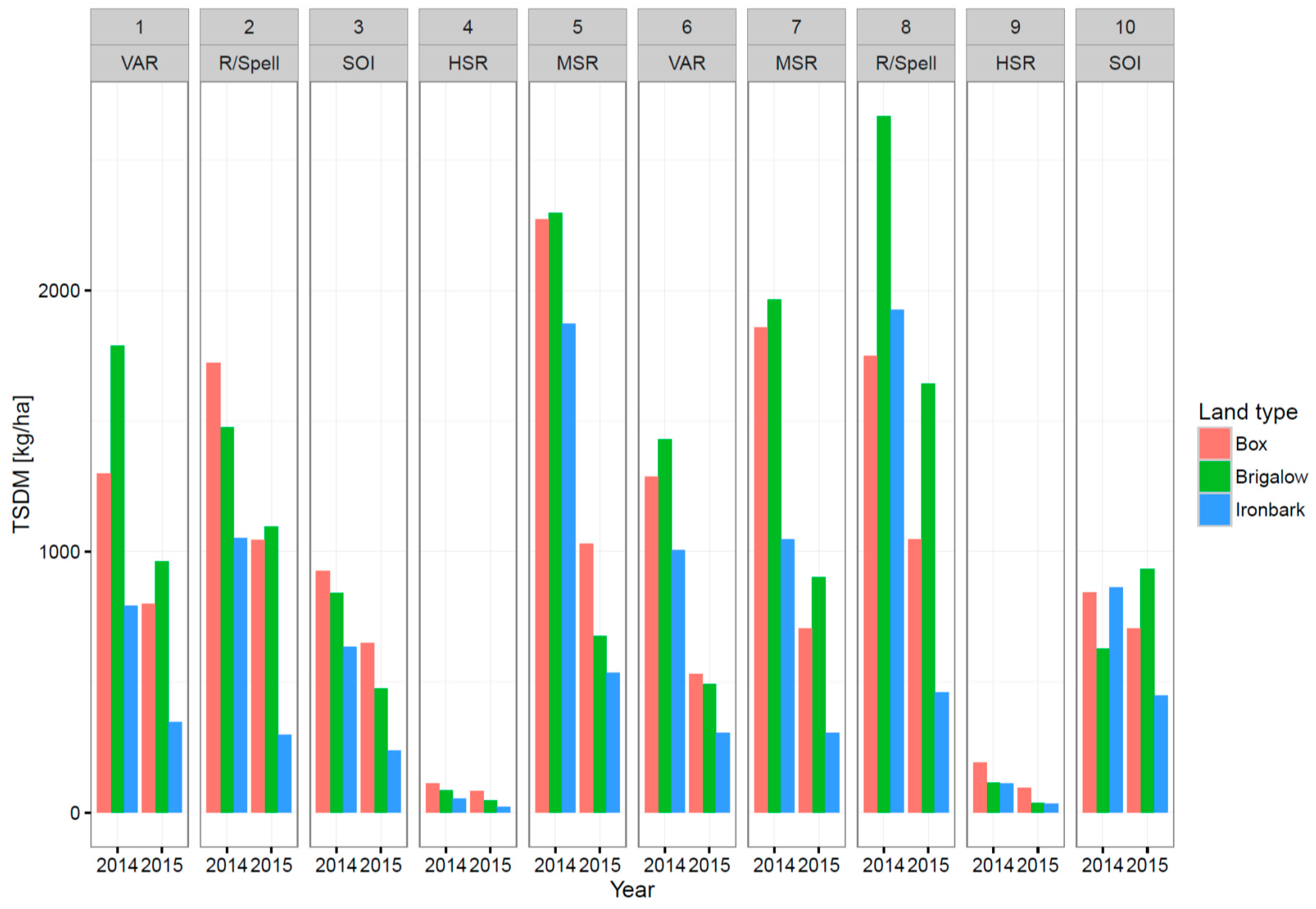
3. Results
The TDSM paddock averages for 2014 and 2015 are displayed in
Figure 3, categorised by paddock (grazing strategy) and land type in the Wambiana grazing trial. TSDM was generally higher at the end of the dry season on October 2014 than at the end of the wet season in May 2015 due to the impact of grazing and a failed wet season. The mean TSDM across all paddocks was 1190 kg/ha for the end of the ‘dry’ season and 612 kg/ha for the end of the ‘wet’ season.
The HSR strategy (highest pasture utilisation) had the lowest TSDM, while the MSR strategy generally displayed the highest TSDM values. An exception to this was the Brigalow land type in Paddock 8 (R/Spell strategy), where high TSDM values were reported in 2014 as well as in 2015. In this paddock and land type there is an artificial topographic feature in the form of a levee bank, which may retain some excess moisture and could explain the higher TSDM values.
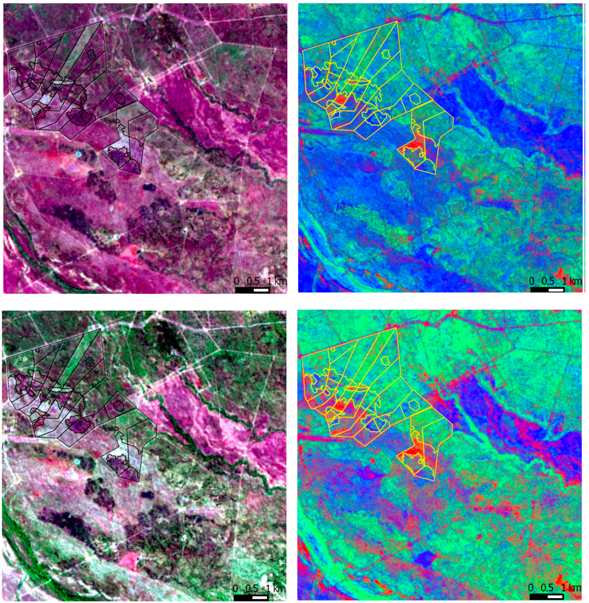
The increase in green cover from October 2014 to May 2015 (
Figure 4) is likely due to an increase in overstorey greenness and not the pastures’ greenness.
The paddocks with different grazing treatments are visible in the R/G/B and the FVC imagery as well as the difference in greenness and vegetative cover between the two seasons.
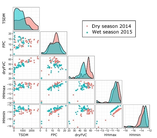
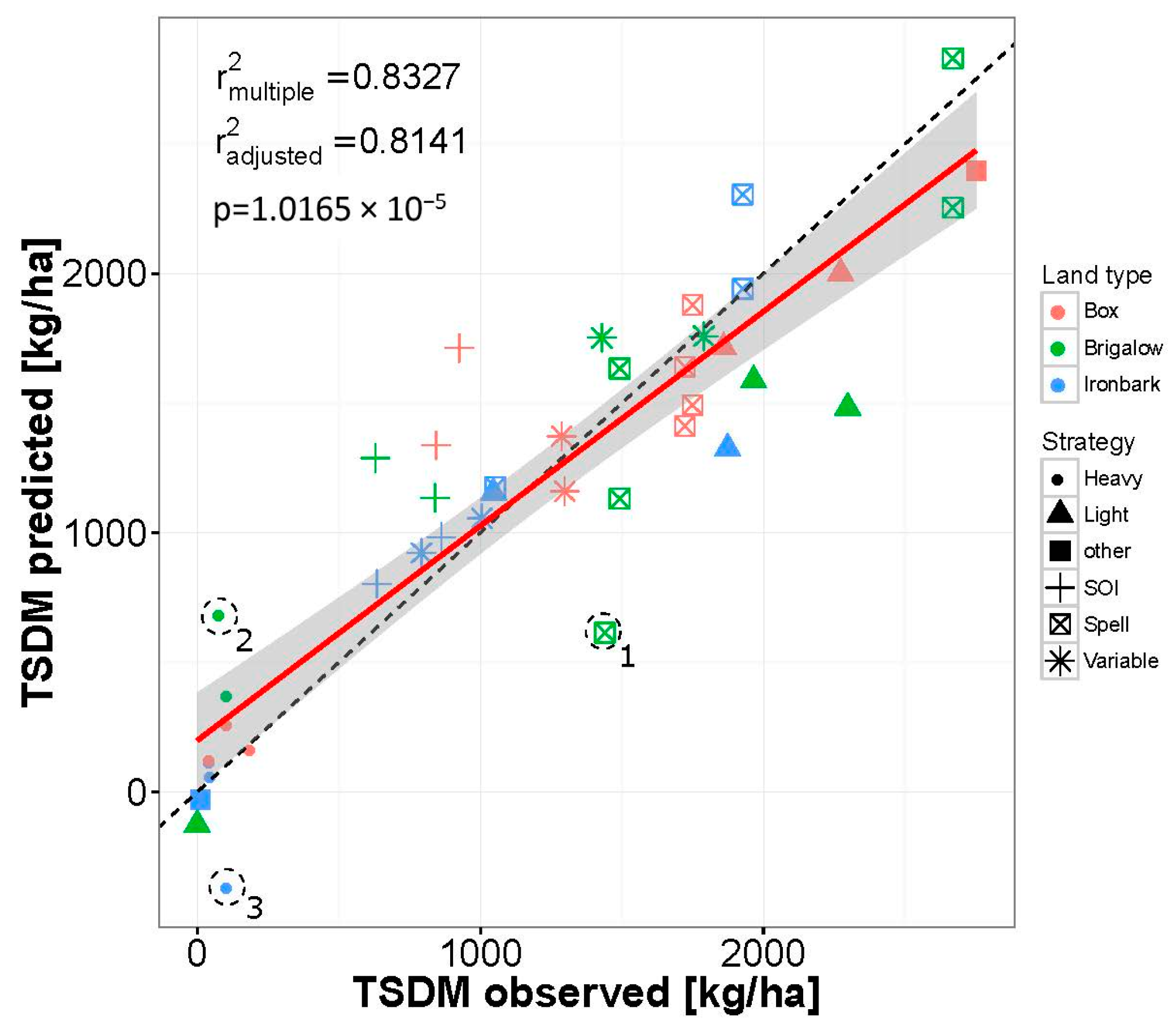
In order to establish a TSDM model from the variables available, several regressions with differing variables were tested. The best-performing and simplest model revealed a robust multiple regression with four variables:
- (1)
FPC;
- (2)
dry fraction of the FVC (dryFVC);
- (3)
the maximum HH (HHmax); and
- (4)
the minimum HH (HHmin).
Without interaction terms: TSDM (dryFVC, FPC, HHmax, HHmin) as shown in
Figure 5. All four variables were highly significant (
p < 0.001).
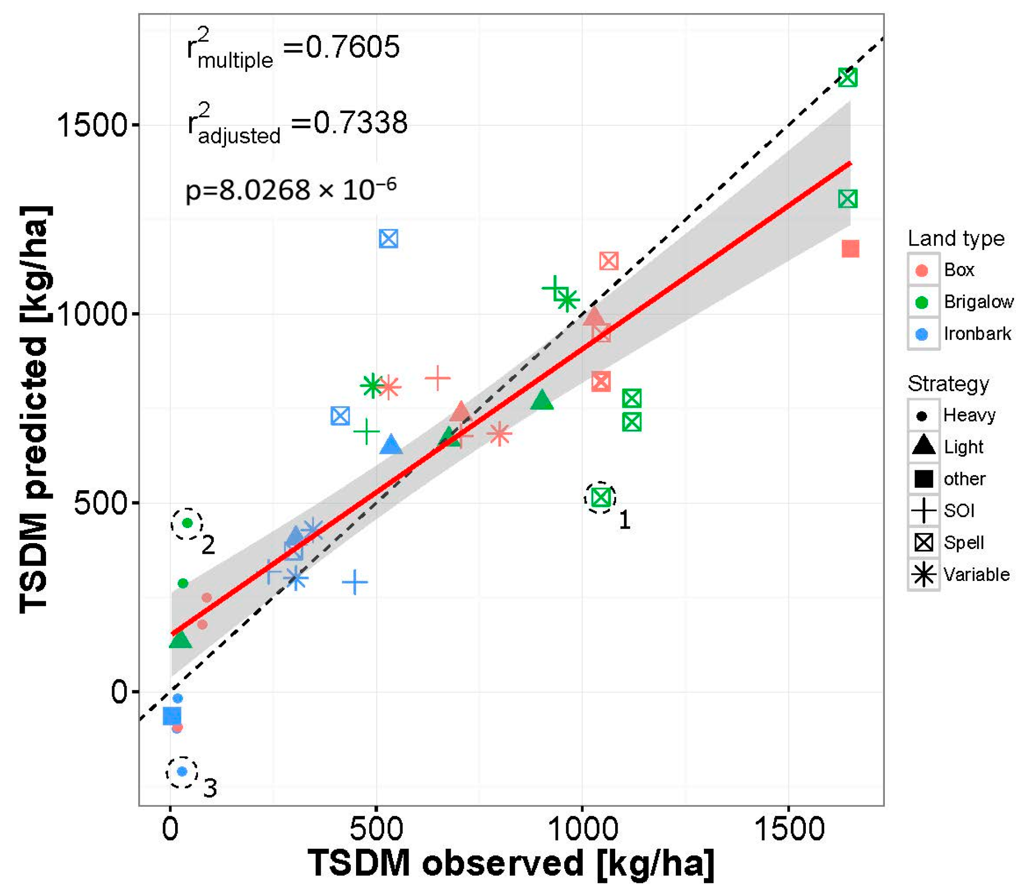
The same variables were used in 2015 for a robust multiple regression for the wet season (
Figure 6). All variables were highly significant (
p < 0.001) with the exception of HHmin (
p < 0.1).
Three data points that appear as outliers in both models are indicated with a dotted circle (
Figure 5 and
Figure 6). Point 1 refers to a small scalded area, approximately 90 m in diameter on Brigalow land type in Paddock 2. Given the nature of the TSDM field data transects, it is conceivable that the observations are too high in both seasons—the transects may not have intersected in this small area and the surrounding high yield box land type area estimates were attributed instead. Point 2 has high predictions in both models, which may be attributable to a levee bank to retain water and the associated disturbed soil when it was established. This would most certainly alter the TSX backscatter signal. Point 3 in both seasons predicted negative TSDM values. It happens that this is the paddock with lowest cover at low FPC and therefore the data point is at the extreme end. The red square represents the grazing exclosure (shown as Ex in
Figure 1) and the blue square is a bare area taken just outside the grazing trial area.
The four input variables were tested for their relevance in predicting TSDM for 2014 and 2015. All variable combinations were tested in multiple regression models.
Table 3 summarises the variable importance and the respective predictive qualities for TSDM via the adjusted r
2 values and the mean residual standard error (MRSE). This was also performed for a model combining all data from both seasons.
As a single variable, dryFVC exhibits the highest correlation with pasture TSDM. The optical data alone (FPC and dryFVC) have r2 values of 0.61 and 0.69 in 2014 and 2015. The r2 increases when adding the HHmax by 6% and 4%, respectively. The addition of HHmin resulted in an increase in r2 of 20% in 2014 and 5% in 2015.
Despite the suspicion of collinearity for HHmin and HHmax reduced the inclusion the model variance for high and low TSDM. An ANOVA for the 2014 data indicated a highly significant model improvement by including either HHmin or HHmax compared to a three-variable model. In 2015 the inclusion of HHmin was significant at the 1% level with a lower p value:
p < 0.05. The inclusion of all other variables was highly significant (
Table 4).
The two models established are different for the dry and the wet season as the environmental conditions differ accordingly.
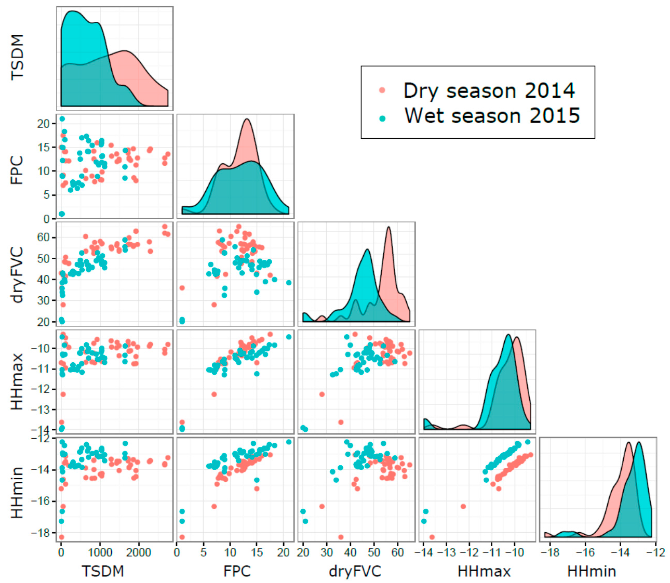
Figure 7 shows the input data separated by season as scatterplots and histograms as a probability density function.
The histogram of TSDM in
Figure 7 reveals a clear difference in the data distribution, with lower TSDM in the 2015 wet season, as indicated in
Figure 3. FPC appears with a different distribution at the high and low end of the distribution. More foliage may have been produced in the over- and midstorey during the wet season. The dryFVC (dry grass and tree litter) is clearly lower in 2015—also visible in
Figure 4. HHmin and HHmax display distinct differences for the wet and dry season. As expected, the two backscatter variables with the same polarisation are correlated. However, the different overpasses and view angles generate sufficient additional information to improve the model performance (
Table 4). The TSX data visually show a relation to FPC, which can be attributed to the interaction of X-band with the leaf canopy.
There appears to be an offset between the 2014 dry season and 2015 wet season data, most evident in the data pairs of FPC and TSX HHmin and also HHmax. The tree species in the study area are likely to exhibit an increase in litter fall and hence reduced FPC during a dry season. In another tropical savanna system, the woody species within crown overstorey FPC changed up to 20% between the wet and dry seasons for some evergreen species and up to 40% when averaged over 49 species including evergreen, partly, and fully deciduous [
40].
This effect would also influence the total leaf water content held in a crown. The overall greenness (FVC green vegetation component) at paddock scale increased by 12.9% from the 2014 dry season to the 2015 wet season, while the FPC only changed 2.9% and the dryFVC declined by 17%.
Table 5 summarises the single-date HH TSX observations and the relation to the respective seasonal FPC dataset. There appear to be a different slope and intercept in a simple regression with wet and dry seasons.
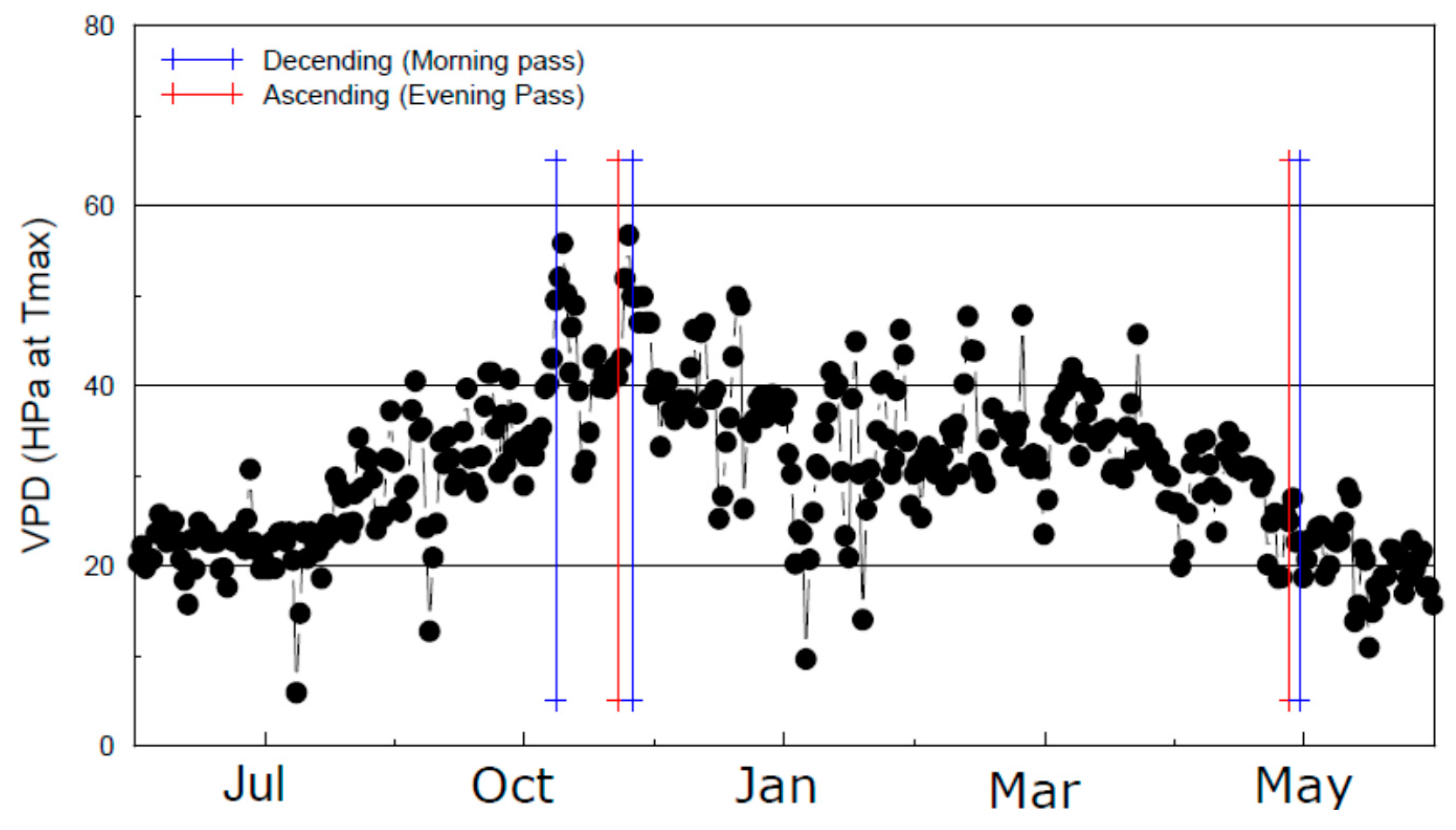
One possible explanation for this disparity is the different levels of moisture in the system. Although the rainfall was very low for both the wet and the dry season, the water vapour deficit was substantially higher in the dry season (
Figure 8). The higher overall greenness, as observed in
Figure 2, also indicates a higher canopy greenness and FPC. It can be assumed that the vegetative water content in the overstorey is also higher, which may influence the HH backscatter signal.
Figure 8 shows the vapour pressure deficit (VPD) in relation to the TSX observations. There is a large difference in the 2014 dry season observation between the descending and ascending overpasses (day, night). In addition to seasonal changes in tree canopy, it is possible that hydroscopic moisture from the atmosphere is influencing backscatter from the soil surface and dead grass.
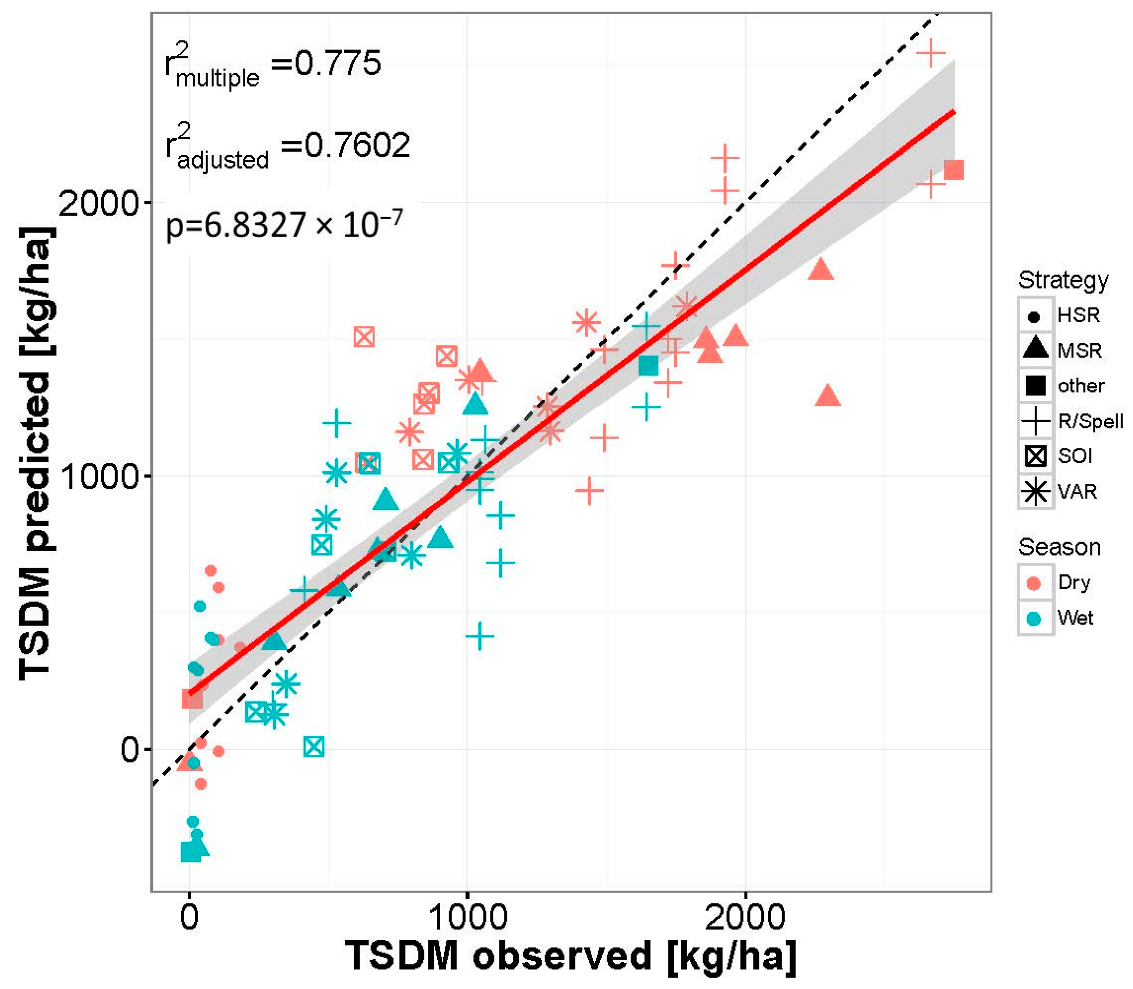
To accommodate the different conditions in the wet and dry season in a more robust manner, a combined model (wet and dry season) was established, where ‘season’ is a factor in the prediction (
Figure 9).
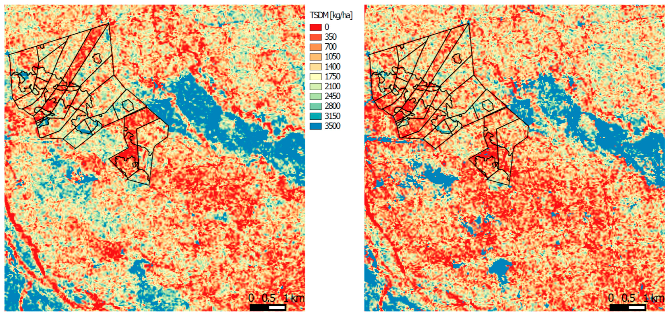
The spatial distribution of the TSDM model output for the grazing trial area is displayed in
Figure 10. The model was restrained to the available data range such that negative predictions were set to zero and the upper values were capped at 3500 kg/ha TSDM.
The TSDM maps for the grazing trial and the surrounding areas (
Figure 10) show a general decrease in TSDM from 2014 to 2015, with some localised deviations. The high stocking rate Paddocks 4 and 9 stand out clearly and are low in comparison to the other grazing strategies, such as the MSR in Paddock 5 and 7, which had the highest TSDM. The Box land type in the HSR paddocks (4 and 9) show a relative increase in TSDM in 2015 compared to 2014, which is in contrast to the field observations (
Figure 3)—though the decrease in field measured TSDM is only 30 kg/ha (Paddock 4) and 98 kg/ha (Paddock 9). The lower TSDM in the other paddocks and land types for 2015, as indicated by the field data in
Figure 3, is also reflected in the TSDM maps (
Figure 10). The only area with higher field observations in TSDM in 2015 compared to 2014 (
Figure 3) is in Paddock 10 on the Brigalow land type, which is also mapped in
Figure 10 with increased TSDM.
4. Discussion
Pasture biomass measurements, in the form of TSDM, at the Wambiana grazing trial were spatially averaged to paddock scale (100 ha) and parcels of land type subdivisions. The spatial averaging of the satellite imagery (TSX, FPC, and FVC) to the paddock and parcel scale makes the satellite observations less spatially explicit, but more precise. This form of noise reduction may have contributed to establishing good relationships in this complex natural environment for a tree-grass ecosystem. A second form of noise reduction in the optical domain was the temporal averaging for the FPC and FVC product across several individual satellite images. In the case of FVC, only Landsat 8 OLI imagery were used, as there appeared to be a calibration difference in the FVC products between Landsat 7 and 8. This effect was not observed in the FPC product, therefore all available Landsat imagery was used in the FPC temporal averaging.
The dry component of FVC is the most important variable in the pasture TSDM estimation, with an r
2 of 0.57 alone, for both the dry season and wet season with TSDM (
Table 3). The generally low vegetative ground cover in 2015 makes dryFVC a relatively good predictor in combination with FPC in low cover areas. However, the dryFVC component incorporates tree leaf litter components and it is unclear how robust the parameters will be in systems with different tree cover, as the cover-to-biomass relationship tends to saturate [
5].
There was a noticeable difference in the overstorey FPC between 2014 and 2015 (
Figure 4) within the study site. The parcel average FPC values did not change much (2.9% difference), but as the greenness in the system is almost exclusively attributable to the overstorey, it appears that with the surplus in greenness (12.9%) there might also be a surplus of vegetative moisture in the overstorey. This additional moisture may have altered the X-band backscatter, resulting in a changed relationship between FPC and HHmin or HHmax (
Table 3,
Figure 7). The variable HHmin appears to have an important influence in this context, so a series of images with differing viewing geometry seems to add to the information content. Only two HH overpasses in 2015 were available for the study region and therefore the difference between HHmax and HHmin was not as pronounced as with three observations in 2014, which may have contributed to a poorer model fit.
The robust multiple regression approach (without interaction terms) has represented the data well for the wet and dry season models as well as the combined model (
Figure 5,
Figure 6 and
Figure 9). The largest scatter in the point clouds appear between 1000 and 2000 TSDM, while the predictions at the low (e.g., <500 TSDM) and high TSDM fit the data better. However, at very low TSDM values (<50 TSDM) some scatter and also negative predicted values appear. This could potentially be avoided by the application of an appropriate data transformation. These points were digitised and may be more error-prone than the TSDM observations.
Pasture utilisation rates resulting from the different stocking regimes in the grazing trial are clearly visible in the modelled TSDM maps for the dry season 2014 and the wet season 2015 (
Figure 10). The relative increase of TSDM in the HSR Paddock 4 and 9 on box land type is in contrast to the field observations, which may be influenced by the relative significance of the FPC in the very low TSDM areas and the influence of the invasive shrub Carissa, which is highest in the box land type of the HSR treatment.
The MRSE was lower for 2015, perhaps because the total TSDM values were lower. A combined model for both seasons was established—with this approach there was some nominal model accuracy (r
2 and MRSE) sacrificed, with the benefit of a more robust model with more data points. The MRSE values for the calibrated dataset are encouraging; however, the MRSE as a percentage of the mean TSDM for dry, wet, and combined seasons is 28%, 41%, and 40% respectively, which is still high relative to the planned pasture usage by cattle (about 20% of annual growth). A 40% error in TSDM estimation is, however, still an improvement over the current state as landholders often have only a vague idea about TSDM on their property as destructive measurements are expensive and impractical. Other forms of TSDM estimates vary greatly between methods, observers, and grass species [
3].
The Wambiana grazing trial is a small study area with relatively good observed field data, with the whole trial site of 10 paddocks (about 1000 ha) being typically about the size of a single paddock in the grazing systems for the region. Upscaling of the findings for wider applications would be desirable, e.g., using TSX ScanSar mode (up to 18.5 m resolution) or Wide ScanSar (up to 40 m resolution) with swath width of approximately 100 km and 270 km, respectively. The HV polarisation did not add significantly to a TSDM model and was thus not included in further analysis. The investigation of quad polarisation may give more insight, or dual polarisation with VV as an additional variable. A time series of X-band imagery over the full duration of a wet and dry season would be ideal to evaluate the ‘within-season’ temporal behaviour. The characterisation of a more general TSDM model would also entice monitoring over longer time spans to cover a range of different seasons temporally, a range of different soil types spatially, and a range of different vegetation types structurally.
In order to apply a TSDM model across a wider area, more field data across space and time would be required. The dataset provided did not include a high proportion of green pasture biomass due to drought conditions and dry soils. The establishment of a pasture biomass data library would be desirable for larger scale studies. The c-band radar from Sentinel-1 may in future provide a useful time series in conjunction with X-band data and optical imagery of high temporal frequency for phenological analysis [
41].


