Improving the Imaging Quality of Ghost Imaging Lidar via Sparsity Constraint by Time-Resolved Technique

Abstract

Ghost imaging via sparsity constraint (GISC)—which is developing into a new staring imaging lidar—can obtain both the range information and spatial distribution of a remote target with the use of the measurements below the Nyquist limit. In this work, schematics of both two-dimensional (2D) and three-dimensional (3D) GISC lidar are introduced. Compared with the 2D GISC lidar, we demonstrate by both simulation and experimentally that the signal-to-noise ratio of the 3D GISC lidar can be dramatically enhanced when a time-resolved technique is used to record the target’s reflection signals and the orthogonal characteristic of the target’s 3D surface structure is taken as a priori in the image reconstruction process. Some characteristics of the 2D and 3D GISC lidar systems are also discussed.

1. Introduction

As an important detection tool, lidar has been widely used in remote sensing in recent decades. Although great progress in remote imaging has been made with methods such as scanning imaging lidar and pulsed floodlight-illumination imaging lidar, the present methods have limitations to either the detection range or the application mode [1,2,3]. Ghost imaging (GI), as a staring method, can nonlocally image an unknown object by using a single-pixel detector at the object path [4,5,6,7,8,9]. Because all the photons reflected (or transmitted) from the object illuminate the same single-pixel detector, this technique has the capability of being highly sensitive in detection, and in recent years, it has aroused increasing interest in remote sensing for the development of a new imaging lidar [10,11,12,13,14,15,16,17,18]. In 2009, when the range from the source plane to the object plane was larger than the distance between the source plane and the camera plane at the reference path, GI could also be obtained, which provided a feasible approach to remote sensing applications [9]. Based on the idea of Reference [9], a two-dimensional ghost imaging lidar via sparsity constraint (2D GISC lidar) was invented, and high-resolution 2D imaging was experimentally demonstrated in 2012 [11,12]. Later, when the time-resolved technique was used to measure the target’s reflection signals, we proposed a three-dimensional ghost imaging lidar via sparsity constraint (3D GISC lidar) system and obtained 3D imagery of a scene at a range of approximately 1.0 km [18]. For both the 2D GISC lidar and 3D GISC lidar, we had used a quite general prior knowledge that all natural objects could be sparsely expressed in a proper representation basis, and several experiments demonstrated that the target’s image could be stably reconstructed by using random measurements far below the Nyquist limit [11,13,18,19,20,21]. In contrast with the 2D GISC lidar, the 3D GISC lidar used the time-resolved technique to detect the target’s reflection signals, which makes the tomographic images at each time delay (namely each depth) become much sparser. Moreover, the target’s spatial structure information was also considered in the process of image reconstruction for the 3D GISC lidar [19]. Therefore, for the same target, the reconstruction quality of the 3D GISC lidar may be significantly enhanced compared with that of the 2D GISC lidar for an equal number of measurements. In this work, we present simulated and experimental demonstrations of image enhancement for the 3D GISC lidar when the time-resolved technique is used, and discuss the characteristics of 2D and 3D GISC lidar systems.

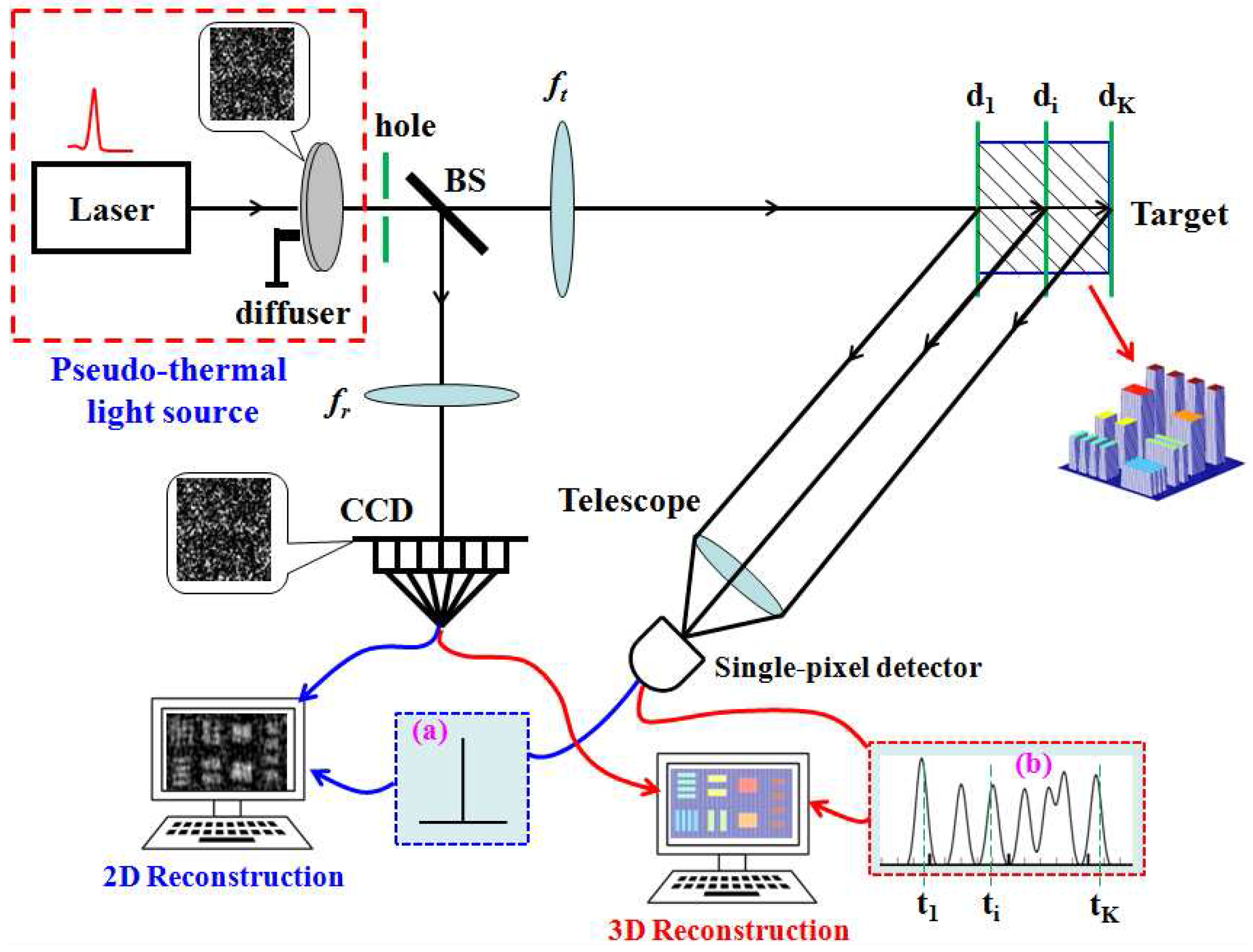
2. Experimental Setup and Image Reconstruction

Figure 1 presents the principle setup of the 2D and 3D GISC lidar systems with a pseudo-thermal light source. The pseudo-thermal light source, which is obtained by passing a pulsed laser beam through a slowly rotating diffuser, goes through a hole and is then divided by a beam splitter (BS) into object and reference paths. In the reference path, a charge-coupled device (CCD) camera is placed on the image plane of the hole. In the object path, the speckle pattern located at the plane of the hole is imaged onto the target by an objective lens $f_t$. The photons reflected from the target are collected by a telescope and then illuminate a single-pixel detector. For the 2D GISC lidar system, the single-pixel detector is a bucket detector without spatial or temporal resolution, while it is a time-resolved bucket detector for the 3D GISC lidar system. In addition, the numerical apertures of the lenses $f_r$ and $f_t$ are the same, which ensures the light fields at the CCD camera plane and the target plane are spatially correlated. According to the intensity distribution recorded by the CCD camera and the signals recorded by the single pixel detector shown in Figure 1a,b, the target’s 2D and 3D images can be reconstructed by the 2D GISC and 3D GISC reconstruction methods [11,19,22,23], respectively.

For 2D GISC reconstruction, we have used the target’s sparsity constraint in a proper representation basis and the target’s gray distribution is always real and nonnegative [11,22,23]. The target’s projection image ${\mathrm{X}}_{2\mathrm{D}}$ can be reconstructed by solving the following convex optimization program [11,22,23]:

$$\begin{array}{c}\hfill {\mathrm{X}}_{2\mathrm{D}}=\mathrm{\Psi }\alpha ;\mathrm{which}\mathrm{minimizes}:\frac{1}{2}{∥{\mathrm{Y}}_{2\mathrm{D}}-{\mathrm{AX}}_{2\mathrm{D}}∥}_2^2+\tau {∥\alpha ∥}_1\end{array}$$

(1)

where A is an $M\times N$ matrix, ${\mathrm{Y}}_{2\mathrm{D}}$ is an $M\times$ 1 column vector, and ${\mathrm{X}}_{2\mathrm{D}}$ is an $N\times$ 1 column vector. Ψ is an $N\times N$ transform operator, and α is an $N\times$ 1 column vector. In addition, τ is a nonnegative parameter, ${∥V∥}_2$ denotes the Euclidean norm of V, and ${∥V∥}_1={\sum }_i\left|{\upsilon }_i\right|$ is the ${\ell }_1$-norm of V.

For 3D GISC reconstruction, apart from the property and constraint used in 2D GISC reconstruction, we have also exploited the orthogonal characteristic of the target’s 3D surface structure [18,19]. That is, as shown in Figure 1, the light reflected by the target in the slice at a certain distance cannot reach the target in the slices behind, such as the green double-slit and the yellow double-slit in Figure 1; namely, the target’s images at different depths have no spatial overlap. The target’s 3D image ${\mathrm{X}}_{3\mathrm{D}}$ can be restored by solving the following convex optimization program [19]:

$$\begin{array}{c}\hfill {\mathrm{X}}_{3\mathrm{D}}=\mathrm{\Psi }\mathrm{O};\mathrm{which}\mathrm{minimizes}:\frac{1}{2}{∥{\mathrm{Y}}_{3\mathrm{D}}-{\mathrm{AX}}_{3\mathrm{D}}∥}_2^2+\tau {∥\mathrm{O}∥}_1+{\tau }_c\mu \left({\mathrm{X}}_{3\mathrm{D}}\right)\end{array}$$

(2)

where A is an $M\times N$ matrix, ${\mathrm{Y}}_{2\mathrm{D}}$ is an $M\times Q$ matrix, and ${\mathrm{X}}_{3\mathrm{D}}$ is an $N\times Q$ matrix. Ψ is an $N\times N$ transform operator and $\mathrm{O}$ is an $N\times Q$ matrix. In addition, $\mu \left({\mathrm{X}}_{3\mathrm{D}}\right)$ denotes the mutual coherence function described by Equation (7) of Reference [19] and ${\tau }_c$ is a parameter determined by the coherence between the tomographic images of neighboring depths.

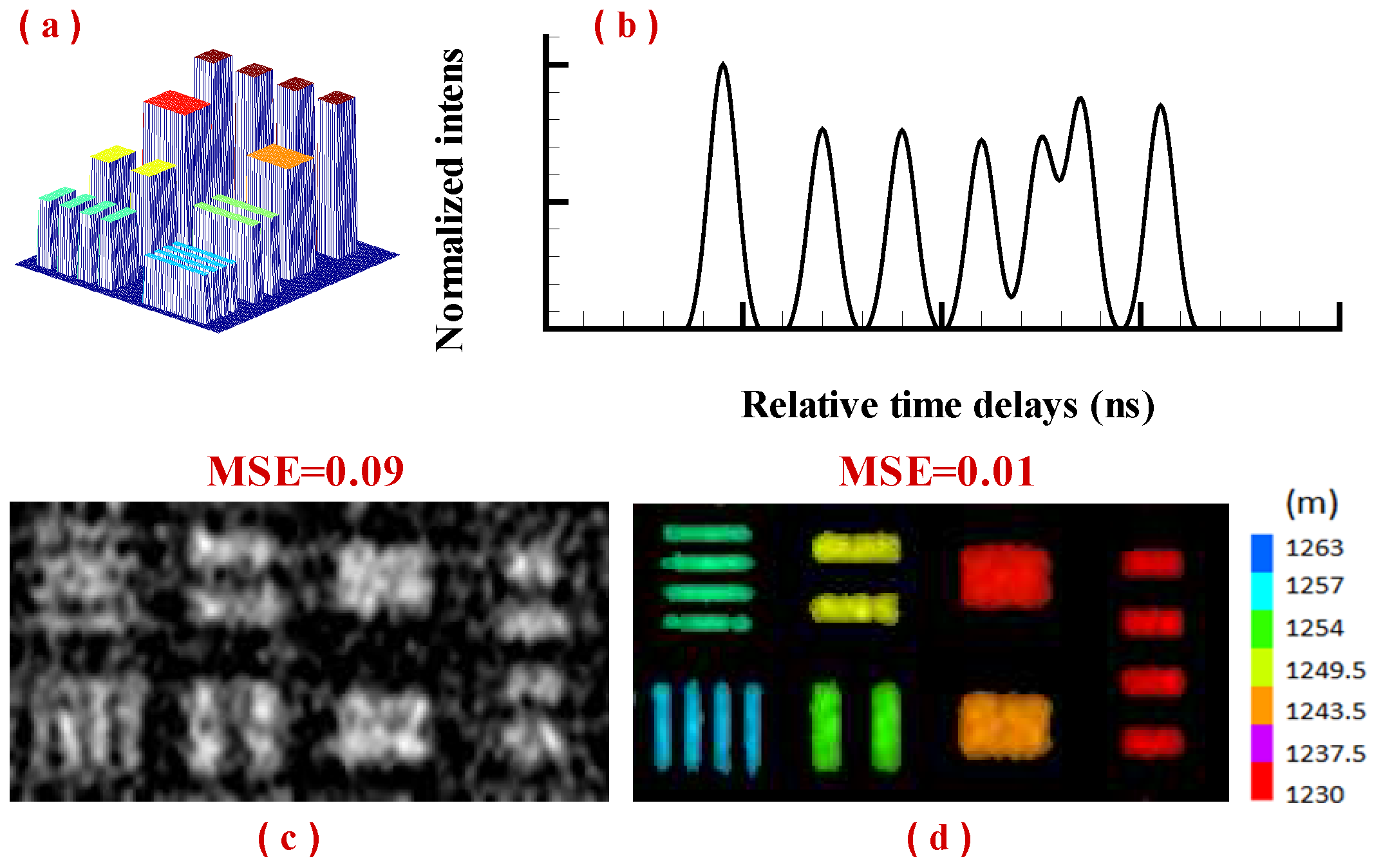
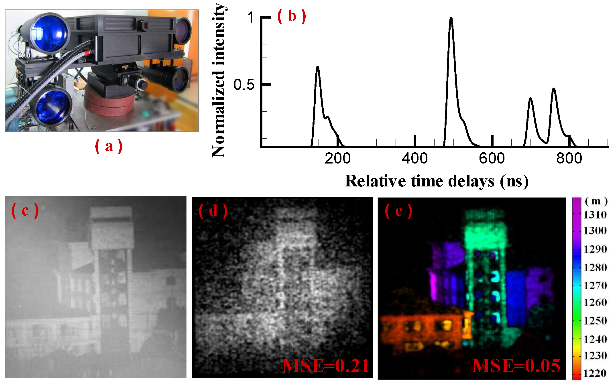
3. Simulation and Experimental Results

To verify the concept, Figure 2 presents simulation results of imaging a series of resolution plates. In the simulation, we used the same parameters provided by the lidar system [18]. The distance between the lidar system and the resolution plate’s front surface ($d_1$ in Figure 1) is 1230 m. The 3D distribution of the resolution plate and the averaged time-resolved signals reflected from the plate are displayed in Figure 2a,b, respectively. In order to keep a good spatial resolution, the pixel size of the CCD camera shown in Figure 1 is set to be nearly half of the speckle’s full width at half-maximum on the CCD plane. For example, the size of the CCD camera used for imaging the resolution plate illustrated in Figure 2a is 200 × 100 pixels, and the number of measurements used for reconstruction is 2000, which yields N $=5000$ resolution cells covering the target (corresponding to 40% of the Nyquist limit) [18,23]. Based on the definition described in Reference [23], the sparse ratio β of the target is 0.22 for the 2D GISC method, whereas in the case of the 3D GISC method, the sparse ratios for the seven time delays are 0.03, 0.03, 0.03, 0.03, 0.03, 0.03 and 0.04. In the process of image reconstruction, the target is represented in a 2D discrete cosine transform basis. For the 2D GISC method, we have utilized gradient projection for a sparse reconstruction algorithm [11,23,24], and the resolution plate’s reconstruction result is illustrated in Figure 2c. For the 3D GISC method, we have employed the fast iterative shrinkage-threshold algorithm [19,25], and the resolution plate’s projection image is shown in Figure 2d. From Figure 2c,d, it is qualitatively seen that 3D GISC reconstruction is much better than 2D GISC reconstruction. To quantitatively evaluate the recovered image’s quality, the mean squared error (MSE) can be calculated with $\mathrm{MSE}=\frac{1}{N_{pix}}{\sum }_{i,j}{\left[I_{2\mathrm{DGISC}/3\mathrm{DGISC}}(x_i,y_j)-I_{\mathrm{o}}(x_i,y_j)\right]}^2$, where $I_{2\mathrm{DGISC}/3\mathrm{DGISC}}$ is the pixel value of recovered 2D GISC or 3D GISC projection images, $I_{\mathrm{o}}$ is the pixel value of the original projection image, and $N_{pix}$ is the total pixel number of the projection image. The calculated MSE values of the images shown in Figure 2c,d are 0.09 and 0.01, respectively. Therefore, when the measurement number is the same and the time-resolved technique is used, the 3D GISC lidar can improve the image’s signal-to-noise ratio (SNR) compared with the 2D GISC lidar, because the tomographic images at each time delay become much sparser.

Here, we present an experimental demonstration of imaging a building located approximately 1200 m away using the lidar system described in Reference [18], as shown in Figure 3a. Figure 3c illustrates the original target captured in one evening by a telescope with receiving aperture 140 mm and focal length 477 mm. Based on the 2D GISC method, the reconstruction result is displayed in Figure 3d. With the use of a time-resolved bucket detector, Figure 3b presents the averaged time-resolved signals reflected from the building, and its projection image reconstructed by the 3D GISC method is shown in Figure 3e. The calculated values of the MSE for the 2D GISC and 3D GISC reconstructions are 0.21 and 0.05, respectively. In addition, according to the definition described in Reference [23], the sparse ratio of the scene is 0.49 for the 2D GISC method. Based on the 3D GISC reconstruction results, we find that the tomographic image located at 1255 m is relatively complex, and the value of the sparse ratio is the largest ($\beta =0.09$), which corresponds to the peak value shown in Figure 3b. Therefore, similar to the simulated results illustrated in Figure 2, the imaging quality of GI lidar can be dramatically enhanced when both the time-resolved technique and the orthogonal characteristics of the target’s 3D surface structure are used.

4. Discussion

For the 2D GISC lidar, because the bucket detector used to record the scene’s reflection signal has no temporal resolution capability, we can only capture the scene’s 2D projection image, losing the depth information of scene [11,12]. Compared with the 2D GISC lidar, the 3D GISC lidar can not only obtain an image with a better SNR in the same random measurement number, but also achieve the scene’s surface 3D image, which is much more advantageous in capturing the characteristics of the targets and has recently attracted increasing attention in remote sensing [18,19,26,27]. As an application in remote sensing, the 3D GISC lidar requires high time resolution and a spatial light diffuser with a high damage threshold. For the former, we usually use a short narrow pulsed laser to illuminate the scene and measure the scene’s signals with a wide-bandwidth single-pixel detector [18,19,26]. A recent report on pulse-compression GI lidar via coherent detection demonstrates that high depth resolution can also be obtained by using a long pulsed laser and low-bandwidth single-pixel detectors [27]. For the latter requirement, some spatial light diffusers, such as rotating ground glass disks, digital micro-mirror devices, and spatial light modulators, are used to modulate the spatial information of the light field in a GISC system [11,12,18,22,23,26,28]. However, both the damage threshold and energy utilization of a rotating ground glass disk are the highest [18,28]. Therefore, the 3D GISC approach mentioned here and in Reference [18] is much more helpful for remote sensing, in contrast with the system demonstrated in [26]. In addition, although the imaging quality can be enhanced by the method of the 3D GISC lidar, the detection range will be less than that of the 2D GISC lidar. This is because the 2D GISC lidar assembles all the signals reflected from the target for each measurement, while for 3D GISC lidar, the signals are divided into a series of slices by the time-resolved bucket detector. Therefore, the 2D GISC lidar has an advantage in the area of remote early warning compared with the 3D GISC lidar. In this paper, we only give the experimental demonstration of a static target, but the principle of GI for a moving target has been verified, and we have just completed the vehicle-mounted 3D GISC lidar experiment [15,16], and the experiment of airborne 3D GISC lidar is preparing. Unfortunately, because the image reconstruction of 3D GISC lidar is a convex optimization process of sparse solution which needs many iterations and is time-consuming, the run times needed for sparse reconstruction is longer than traditional intensity correlation reconstruction algorithm of GI, and much longer than traditional scanning imaging lidar and pulsed floodlight-illumination imaging lidar [1,2,3,18,19,22,23]. However, the measurements needed for 3D GISC reconstruction can be obviously decreased, which is helpful for fast imaging and the image acquisition of a high-speed moving target. In addition, we have simply illustrated the 3D image of a target, and the image representation of 3D GISC will be one of our research focuses in the next work.

5. Conclusions

In conclusion, we experimentally show that both the 2D GISC lidar and 3D GISC lidar can obtain a target’s image with the use of random measurements below the Nyquist limit (usually less than 70% of the Nyquist limit). When the time-resolved technique is introduced to record the target’s reflection signals and the orthogonal property of the target’s 3D surface structure is used in the process of image reconstruction, we also demonstrate that the reconstruction SNR of 3D GISC lidar is four times higher than that of the 2D GISC lidar (evaluated by MSE) for the same number of measurements.

References

1. Richmond, R.D.; Cain, S.C. Direct-Detection Ladar System; TT85; SPIE Publications: Bellingham, WA, USA, 2009; pp. 117–132. [Google Scholar]
2. Yun, J. High-peak-power, single-mode, nanosecond pulsed, all-fiber laser for high resolution 3D imaging lidar system. Chin. Opt. Lett. 2012, 10, 121402. [Google Scholar]
3. Anthes, J.P.; Garcia, P.; Piercs, J.T.; Dressendorfer, P.V. Nonscanned ladar imaging and applications. Proc. SPIE 1993, 1936, 11–22. [Google Scholar]
4. Bennink, R.S.; Bentley, S.J.; Boyd, R.W.; Howell, J.C. Quantum and classical coincidence imaging. Phys. Rev. Lett. 2004, 92, 033601. [Google Scholar] [CrossRef] [PubMed]
5. Cao, D.Z.; Xiong, J.; Wang, K. Geometrical optics in correlated imaging systems. Phys. Rev. A 2005, 71, 013801. [Google Scholar] [CrossRef]
6. Zhang, D.; Zhai, Y.-H.; Wu, L.-A.; Chen, X.-H. Correlated two-photon imaging with true thermal light. Opt. Lett. 2005, 30, 2354–2356. [Google Scholar] [CrossRef] [PubMed]
7. Ferri, F.; Magatti, D.; Gatti, A.; Bache, M.; Brambilla, E.; Lugiato, L.A. High-resolution ghost image and ghost diffraction experiments with thermal light. Phys. Rev. Lett. 2005, 94, 183602. [Google Scholar] [CrossRef] [PubMed]
8. Angelo, M.D.; Shih, Y.H. Quantum imaging. Laser Phys. Lett. 2005, 2, 567–596. [Google Scholar] [CrossRef]
9. Gong, W.; Zhang, P.; Shen, X.; Han, S. Ghost “pinhole” imaging in Fraunhofer region. Appl. Phys. Lett. 2009, 95, 071110. [Google Scholar] [CrossRef]
10. Erkmen, B.I. Computational ghost imaging for remote sensing. J. Opt. Soc. Am. A 2012, 29, 782–789. [Google Scholar] [CrossRef] [PubMed]
11. Zhao, C.; Gong, W.; Chen, M.; Li, E.; Wang, H.; Xu, W.; Han, S. Ghost imaging lidar via sparsity constraints. Appl. Phys. Lett. 2012, 101, 141123. [Google Scholar] [CrossRef]
12. Chen, M.; Li, E.; Gong, W.; Bo, Z.; Xu, X.; Zhao, C.; Shen, X.; Xu, W.; Han, S. Ghost imaging lidar via sparsity constraints in real atmosphere. Opt. Photonics J. 2013, 3, 83–85. [Google Scholar] [CrossRef]
13. Gong, W.; Bo, Z.; Li, E.; Han, S. Experimental investigation of the quality of ghost imaging via sparsity constraints. Appl. Opt. 2013, 52, 3510–3515. [Google Scholar] [CrossRef] [PubMed]
14. Hardy, N.D.; Shapiro, J.H. Computational ghost imaging versus imaging laser radar for three dimensional imaging. Phys. Rev. A 2013, 87, 023820. [Google Scholar] [CrossRef]
15. Li, E.; Bo, Z.; Chen, M.; Gong, W.; Han, S. Ghost imaging of a moving target with an unknown constant speed. Appl. Phys. Lett. 2014, 104, 251120. [Google Scholar] [CrossRef]
16. Li, X.; Deng, C.; Chen, M.; Gong, W.; Han, S. Ghost imaging for an axially moving target with an unknown constant speed. Photonics Res. 2015, 3, 153–157. [Google Scholar] [CrossRef]
17. Xu, X.; Li, E.; Shen, X.; Han, S. Optimization of speckle patterns in ghost imaging via sparse constraints by mutual coherence minimization. Chin. Opt. Lett. 2015, 13, 071101. [Google Scholar]
18. Gong, W.; Zhao, C.; Yu, H.; Chen, M.; Xu, W.; Han, S. Three-dimensional ghost imaging lidar via sparsity constraint. Sci. Rep. 2016, 6, 26133. [Google Scholar] [CrossRef] [PubMed]
19. Yu, H.; Li, E.; Gong, W.; Han, S. Structured image reconstruction for three-dimensional ghost imaging lidar. Opt. Express 2015, 23, 14541–14551. [Google Scholar] [CrossRef] [PubMed]
20. Donoho, D.L. Compressed sensing. IEEE Trans. Inf. Theory 2006, 52, 1289–1306. [Google Scholar] [CrossRef]
21. Candès, E.J.; Wakin, M.B. An introduction to compressive sampling. IEEE Signal Process. Mag. 2008, 25, 21–30. [Google Scholar] [CrossRef]
22. Katz, O.; Bromberg, Y.; Silberberg, Y. Compressive ghost imaging. Appl. Phys. Lett. 2009, 95, 131110. [Google Scholar] [CrossRef]
23. Du, J.; Gong, W.; Han, S. The influence of sparsity property of images on ghost imaging with thermal light. Opt. Lett. 2012, 37, 1067–1069. [Google Scholar] [CrossRef] [PubMed]
24. Figueiredo, M.A.; Nowak, T.R.D.; Wright, S.J. Gradient projection for sparse reconstruction: Application to compressed sensing and other inverse problems. IEEE J. Sel. Top. Signal Proc. 2007, 1, 586–597. [Google Scholar] [CrossRef]
25. Beck, A.; Teboulle, M. A fast iterative shrinkage-thresholding algorithm for linear inverse problems. SIAM J. Imaging Sci. 2009, 2, 183–202. [Google Scholar] [CrossRef]
26. Sun, M.; Edgar, M.P.; Gibson, G.M.; Sun, B.; Radwell, N.; Lamb, R.; Padgett, M.J. Single-pixel three-dimensional imaging with time-based depth resolution. Nat. Commun. 2016, 7, 12010. [Google Scholar] [CrossRef] [PubMed]
27. Deng, C.; Gong, W.; Han, S. Pulse-compression ghost imaging lidar via coherent detection. Opt. Express 2016, 24, 25983–25994. [Google Scholar] [CrossRef] [PubMed]
28. Mei, X.; Gong, W.; Yan, Y.; Han, S.; Cao, Q. Experimental research on prebuilt three-dimensional imaging lidar. Chin. J. Lasers 2016, 43, 0710003. [Google Scholar]
Figure 1. Schematic of 2D and 3D GISC lidar (ghost imaging lidar via sparsity constraint) with a pseudo-thermal light source. (a) The signal recorded by the bucket detector for a 2D GISC lidar system; (b) The signal recorded by the time-resolved bucket detector for a 3D GISC lidar system. BS: beam splitter; CCD: charge-coupled device camera.
Remotesensing 08 00991 g001
Figure 2. Simulation results of imaging a series of resolution plates located about 1230 m away, using 2000 measurements. (a) The original distribution of the resolution plate; (b) The averaged time-resolved signals reflected from the resolution plate; (c) The 2D GISC reconstruction result and (d) the plate’s projection image restored by 3D GISC method. The different colors of the image shown in (d) express different detection distances between the objective lens and the target. MSE: mean squared error.
Remotesensing 08 00991 g002
Figure 3. Experimental demonstration results of imaging a building (256 × 256 pixels) at about 1200 m range, using 10,000 measurements (61% of the Nyquist limit). (a) Picture of the invented GISC lidar system; (b) Averaged time-resolved signals reflected from the building; (c) The original target imaged by a telescope with the receiving aperture 140 mm and the focal length 477 mm; (d) 2D GISC reconstruction; (e) The building’s projection image restored by 3D GISC method. The different colors of the image shown in (e) express different detection distances between the objective lens and the target. MSE: mean squared error.
Remotesensing 08 00991 g003