1. Introduction
Hyperspectral images can provide rich information both from the spectral and spatial domain simultaneously. For this reason, hyperspectral images are widely used in agriculture, environmental management and urban planning. Classification of each pixel in hyperspectral imagery is a common method used in these applications. However, hyperspectral sensors generally have more than 100 spectral bands for each pixel (e.g., AVIRIS, Reflective Optics System Imaging Spectrometer (ROSIS)), and the interpretation of such high dimensionality imagery with good accuracy is rather difficult.
Recently, sparse representation [
1] has been demonstrated as a useful tool for high dimensional data processing. It is also widely applied in hyperspectral imagery classification [
2,
3,
4]. Sparse models intend to represent most observations with linear combinations of a small set of elementary samples, often referred to as atoms, chosen from an over-complete training dictionary. In this way, hyperspectral pixels, which lie in a high dimension space, can be approximately represented by a low dimension subspace structured by dictionary atoms from the same class. Therefore, given the entire training dictionary, an unlabeled pixel can be sparsely represented by a specific linear combination of atoms. Finally, according to the positions and values of the sparse coefficients of the unlabeled pixel, the class label can be determined.
Spatial information is an important aspect in sparse representations of hyperspectral images. It is widely accepted that a combination of spatial and spectral information provides significant advantages in terms of improving the performance of hyperspectral image representation and classification (e.g., [
5,
6]). To explore effective spatial features, several methods have been developed in this direction. In [
3], two kinds of spatial-based sparse representation are proposed for hyperspectral image processing. Among them, one is a local contextual-based method. In this method, it adds a spatial smoothing term in the optimization formulation during the sparse reconstruction process of the original data. The second one jointly utilizes the sparse constraints of neighboring pixels, around the pixel of interest. The experimental results show that these two strategies perform better, in terms of classification results. However, both spatial smoothing and the joint sparsity model lay emphasis only on local consistency in the spectral domain, whereas spatial features (e.g., shapes and textures) also need to be explored for better representation of hyperspectral imagery. Recently, mathematical morphology (MM) methods [
7] have been commonly used for modeling the spatial characteristics of the objects in hyperspectral images. For panchromatic images, derivative morphological profiles (DMPs) [
8] have been successfully used for image classification. In the field of hyperspectral image interpretation, spatial features are commonly extracted by building extended morphological profiles (EMPs) [
9] on the first few principal components. Moreover, extended morphological attribute profiles (EMAPs) [
10], similar to EMPs, have been introduced as an advanced algorithm to obtain detailed multilevel spatial features of high resolution images generated by the sequential application of various spatial attribute filters that can be used to model different kinds of structural information. Such morphological spatial features, which are generated from the pixel level (low level), suffer heavily from redundancy and great variations in feature representation. To reduce the redundancy in morphological feature space, several studies have been set to find more representative spatial features by using a sparse coding technique, such as [
11,
12]. However, due to the variability of low-level morphological features, which limited the power of sparse representation, it is necessary to find higher level and more robust spatial features.
To explore higher level and more effective spatial features, [
13] defines sparse contextual properties based on over-segmentation results, which greatly reduce computational cost. However, objects seldom belong to only one superpixel because of the spectral variations, and this is particularly so in high resolution images. Moreover, the spatial features, defined at the superpixel level, are commonly merged and linearly transformed from low level (pixel-level) ones; therefore, they probably would not significantly increase the representation power of spatial features in remote sensing images. After all, both MM and object-level spatial features require prior knowledge of setting proper parameters for feature extraction. The process of parameter setting always produces inefficient and redundant spatial features [
14,
15]. Therefore, in this paper, instead of setting spatial features, we explore high level spatial features by using a deep learning strategy [
16,
17]. Deep learning, as one of the state-of-the-art algorithms in the computer vision field, shifts the human-engineered feature extraction process to automatic feature learning and highly application-dependent feature exploration [
18,
19,
20]. Furthermore, due to the deep structure in such learning strategies (e.g., stacked autoencoder (SAE) [
21], convolutional neural network (CNN) [
22]), one can extract higher level spatial features by using non-linear activation functions, layer by layer, which are much more robust and effective than low level ones. Recently, some efforts have been made in deep learning for hyperspectral image classification. Chen [
23] probably is the first one to explore the SAE framework for hyperspectral classification. In his work, SAE was used for spectral and spatial feature extraction in the hierarchical structure. However, SAE can only extract higher level features from one-dimensional data, while it overlooked the two-dimensional spatial characteristics (although an adjacent effect has been considered). Unlike SAE, CNN takes a fixed size image patch, called the “receptive field”, for deep spatial feature extraction; thus, it can keep spatial information intact. In the work of Chen [
24], wherein the vehicles on the roads are detected by deep CNN (DCNN), the results show that CNN is effective for object detection in high resolution images. Instead of object detection, Yue [
14,
25] explored both spatial and spectral features in higher levels by using a deep CNN framework for the possible classification of hyperspectral images. However, the extracted deep features still remain in a high dimensional space, which involves a rather high computational cost and may lead to lower classification accuracies.
In this paper, we follow a different strategy, exploit the low dimensional structure of high level spatial features and perform sparse representation using both spectral and spatial information for hyperspectral image classification. Specifically, we focus on CNN, which offers the potential to describe the structural characteristics in high levels according to the hierarchical feature extraction procedure. At the same time, we also exploit the fact that the deep spatial features of the same class lie in a low-dimensional subspace or manifold and can be expressed by linear sparse regression. Thus, it would be worthwhile to combine sparse representation with high dimensional deep features, which may provide better representation in terms of the characterization of spatial and spectral features and for better discrimination between different classes. Therefore, the method proposed in this paper for hyperspectral image classification combines the merits of deep learning and sparse representations. In this work, we tested our method on two well-known hyperspectral datasets: an Airborne Visible Infra-Red Imaging Spectrometer (AVIRIS) scene over Indian Pines, IN, USA, and a Reflective Optics System Imaging Spectrometer (ROSIS) scene over Pavia University. The experimental results show that the proposed method can effectively exploit the sparsity that lies at a higher level spatial feature subspace and also provides better classification performance. The merits of the proposed method are as follows: (1) instead of manually setting spatial features, we use CNN to learn such features automatically, which is more effective for hyperspectral image representation; (2) the hierarchical network strategy is applied to explore higher level spatial features, which are more robust and effective for classification compared to the low level spatial features; (3) the sparse representation method is introduced to exploit a suitable subspace for high dimension spatial features, which reduces the computational cost and increases feature discrimination between classes.
The remainder of the paper is structured as follows.
Section 2 presents the proposed methodology in two parts: CNN deep feature extraction and sparse classification and describes the datasets used for experiments and compares the performance of the proposed method with that of other well-known approaches. Finally,
Section 3 concludes with some suggestions for future works.
2. Proposed Methodology
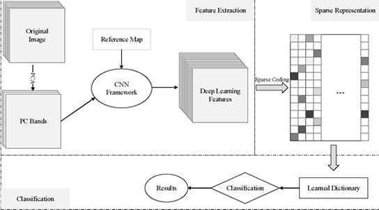
The proposed method can be divided mainly into three parts, as shown in
Figure 1. First, the high level spatial features are extracted by the CNN framework. Then, the sparse representation technique was applied to reduce the dimensionality of the high level spatial features generated by the previous step. Finally, with the learned sparse dictionary, classification results can be obtained.
Figure 1.
Graphical illustration of the convolutional neural networks (CNN)-based spatial feature extraction, sparse representation and classification of hyperspectral images.
Figure 1.
Graphical illustration of the convolutional neural networks (CNN)-based spatial feature extraction, sparse representation and classification of hyperspectral images.
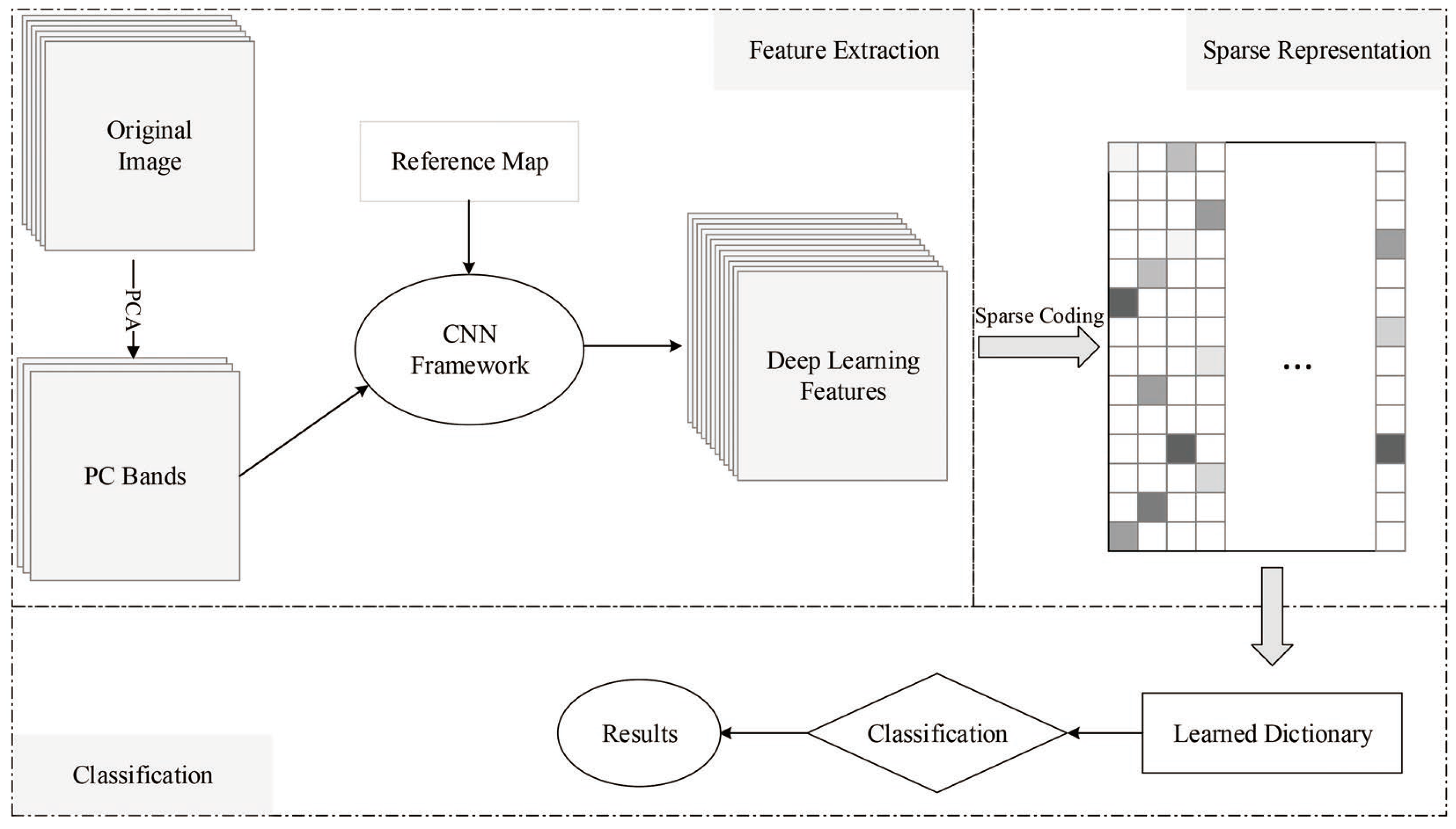
2.1. CNN-Based Deep Feature Extraction
Recently, deep learning, one of the state-of-the-art techniques in the field of computer vision, has demonstrated impressive performances in recognition and classification of several famous image datasets [
26,
27]. Instead of setting image features, CNN can automatically learn higher level features from a hierarchical neural network in a way similar to the process of human cognition. To explore such spatial information, a fixed size of the neighborhood area (receptive field) should be first given. For a PC band of hyperspectral images, given a training sample
and its pixel neighbors in
, a local neighborhood area forms with the size of
; the patch-based training sample can be denoted as
. Additionally, the label of patch sample
can be denoted as
. CNN works like a black box; given the input patches and its labels, the hierarchical spatial features can be generated by a layer-wise activation structure, shown in
Figure 2. Conventionally, two kinds of layers are stacked together in the CNN framework
; the convolution layer and the sub-sampling layer [
28]. Here,
is the non-linear activation function. The convolution layer generates spatial features by activating the output value of previous layers with spatial filters. Then, the sub-sampling layer generates more general and abstract features, which greatly reduces the computational cost and increases the generalization power for image classification. Learning a CNN network with
L layers involves learning the trainable parameters in each layer of the framework. The feature maps of the previous layer are convolved by the convolution layer with learnable kernel
k and bias term
b through the activation function to form feature maps of the current layer. For
l-th convolution layer
, we have that:
where
represents the feature maps of the current layer and
means the feature map lies in the previous layer.
k and
b are trainable parameters in the convolution layer. Commonly, sub-sampling layers are interspersed with convolution layers for computational cost reduction and feature generalization. Specifically, a subsampling layer produces downsampled versions of the input feature maps for feature abstraction. For example, for the
q-th sub-sampling layer
, we have:
where
represents the sub-sampling function that shrinks a feature map by using a mean value pooling operation and
b is the bias term of the sub-sampling layer. The final output layer can be defined as:
where
is the predicted value of the entire CNN and
means the output feature map of the
-th hidden layer in the CNN, which could be either a convolution layer or a sub-sampling layer. During the training process, the squared loss function is applied to measure the deviation from target labels and predicted labels. If there are
N training samples, the optimization problem is to minimize the loss function
as follows:
where
denotes a single activation unit. To minimize the loss function, a backward propagation algorithm is a common choice. Specifically, the stochastic gradient descent algorithm (SGD) is applied to optimize the parameters
k and
b.
The parameter of the entire network could be updated according to the derivatives. Once the back propagation process is finished, k and b are determined. Then, a feed-forward step is applied to generate new error derivatives, which can be used for another round for parameter updating. These feed-forward and back-propagation processes are repeated until convergence is achieved, and thus, optimal k and b are obtained. High level spatial features can thus be extracted by using such learned parameters and a hierarchical framework.
Once the output feature map of the last layer is obtained, it is important to flatten the feature map into a one-dimension vector for pixel-based classification. Therefore, the flattened deep feature can be represented as , where O is the final output feature map.
Figure 2.
The process of CNN-based spatial feature extraction. The training samples are squared patches. The convolution layer and sub-sampling layer are interspersed in the framework of CNN.
Figure 2.
The process of CNN-based spatial feature extraction. The training samples are squared patches. The convolution layer and sub-sampling layer are interspersed in the framework of CNN.
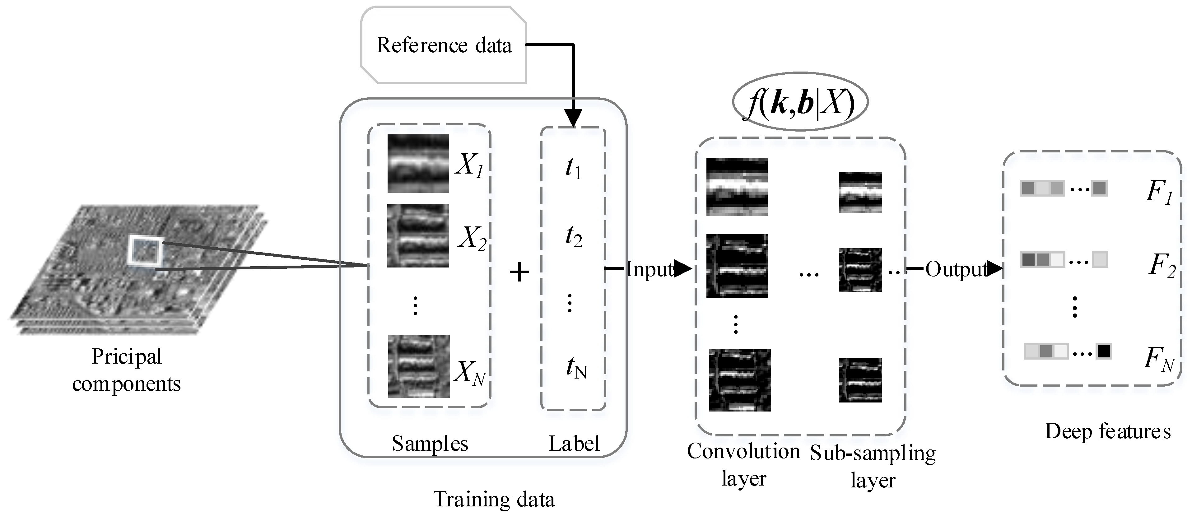
2.2. Deep Feature-Based Sparse Representation
Deep spatial features generated by the CNN framework are usually of high dimensionality, which are ineffective for classification. Therefore, we introduce sparse coding as one of the-state-of-art techniques to find a subspace for deep feature representation and to possibly improve the classification performances, as shown in
Figure 3. The sparse representation classification (SRC) framework was first introduced for face recognition [
29]. Similarly, in hyperspectral images, a particular class with high dimensional features both in the spectral and spatial domain should lie in a low dimensional subspace spanned by dictionary atoms (training pixels) of the same class. Specifically, an unknown test pixel can be represented as a linear combination of training pixels from all classes. As a concrete example, let
be the pixel with
M denoting the dimension of deep features in
D and
the structural dictionary, where
holds the samples of class
c in its columns;
C is the number of classes,
is the number of samples in
; and
is the total number of atoms in
. Therefore, a pixel
, whose class identity is unknown, can be represented as a linear combination of atoms from the dictionary
:
where
is a sparse coefficient for the unknown pixel
. Given the structural dictionary
, the sparse coefficient
α can be obtained by solving the following optimization problem:
where
denotes the
-norm of
α, which counts the number of nonzero components on the coefficient vector, and
δ is the error tolerance, which represents noise and possible modeling error. However, the aforementioned problems make it hard to solve this optimization problem because of its nondeterministic and NP-hard characteristic. To tackle this problem, therefore, greedy algorithms, such as basis pursuit (BP) [
30] and orthogonal matching pursuit (OMP) [
31], have been proposed. In the BP algorithm, the
norm replaces the
norm. The optimization problem is transferred into:
where
K is the sparsity level, representing the number of selected atoms in the dictionary.
, for
. On the other hand, the OMP algorithm incorporates the following steps at each iteration based on the correlation between the dictionary
and the residual vector
, where
. Specifically, at each iteration, the OMP finds the index of the atom that best approximates the residual, adds this member to the matrix of atoms, updates the residual and computes the estimate of
α using the newly-obtained atoms. Once the approximation error falls below a certain prescribed limit, then OMP finds the sparse coefficient vector
. The class label for
can be determined by the minimal representation error between
and its approximation from the sub-dictionary of each class:
Therefore, we proposed the deep feature-based OMP algorithm to explore the low dimension subspace for deep feature representation and for image classification.
Figure 3.
The process of deep feature-based sparse representation classification.
Figure 3.
The process of deep feature-based sparse representation classification.
| Algorithm 1 Framework of the deep feature-based sparse coding. |
| Require: |
| , training pixels from all classes with deep features; A, structural dictionary; C, number of classes; |
| K, sparsity level; |
| Ensure: |
| , sparse coefficients matrix; |
| 1: Initialization: set the index matrix , residual matrix , the iteration counter iter = 1; |
| 2: Compute residual correlation matrix ; |
| 3: Select a new adaptive set based on |
| 4: Find the best representation atoms’ indexes and the corresponding coefficient values for each class c. |
| 5: Combine the best representative atoms for each class into a cluster , and obtain the corresponding coefficients in that cluster. |
| 6: Select the adaptive set from the best atoms out of according to the indexes in . |
| 7: Combine the newly-selected adaptive set with the previously-selected adaptive sets: |
| 8: Calculate the sparse representation coefficients . |
| 9: Update the residual matrix: . |
| 10: Check if sparsity coefficient ; stop the procedures; and output the final sparse coefficient matrix; otherwise, set and go to Step 2. |
2.3. Datasets
In this section, we evaluate the performance of the proposed deep feature-based sparse classification algorithm on two hyperspectral image datasets, i.e., the Reflective Optics System Imaging Spectrometer (ROSIS-03) University of Pavia data and the Airborne Visible/Infrared Imaging Spectrometer (AVIRIS) Indian Pines data.
The AVIRIS Indian Pines image was captured over the agricultural Indian Pine test site located in the northwest of Indiana. Two-thirds of the site contain agricultural crops and one-third forest or other natural, perennial vegetation. The spectral range includes 220 spectral bands from 0.2 to 2.4 μm, and each band measures 145 × 145 with a spatial resolution of 20 m. Prior to commencing the experiments, the water absorption bands were removed. There are 16 different classes in Indian Pines reference map, and most of them can be related to different types of crops.
The University of Pavia image was acquired by the ROSIS-03 sensor over the University of Pavia, Italy. The image measures 610 × 340 with a spatial resolution of 1.3 m per pixel. There are 115 channels whose coverage ranges from 0.43 to 0.86 μm. Prior to commencing the experiment, 12 absorption bands were discarded because of noise. Nine information classes were considered for this scene.
2.4. Configuration of CNN
During the deep feature extraction process, it is important to address the configuration of the deep learning framework. The receptive field (
), the kernel (
k), the number of layers (
) and the number of feature maps of each layer (
) are primary variables that affect the quality of deep features. We empirically set the size of the receptive field to
, which offered enough contextual information. The kernel sizes recommended in recent studies for CNN framework are
,
or
[
32]. For
and
kernels, there were 49 and 81 trainable parameters, which significantly increased the computational cost during training of such a framework, as compared to the cost for
kernels. Therefore, for our CNN framework, we adopted
kernels to accelerate the training process. Once the sizes of the receptive field and kernels are determined, the main structure of the CNN framework can be considered established. A training patch
(receptive field) can generate four levels of feature maps (two convolutional layers and two subsampling layers), and the size of the final output map is
(((28 − (5 − 1))/2 − 4)/2). However, the number of feature maps (
) of each layer still remains unsolved. To solve this problem, we constrained the number of feature maps to be equal at each layer. With this configuration, CNN works, like the deep Boltzmann machine (DBM) [
33], which should not significantly affect the quality of the output of deep features. To illustrate the impact of different CNN configurations on classification accuracy, we conducted a series of experiments, as will be explained in the following section. The experiment was conducted on the spatially independent training sets and the remaining as the test datasets.
2.4.1. CNN Depth Effect
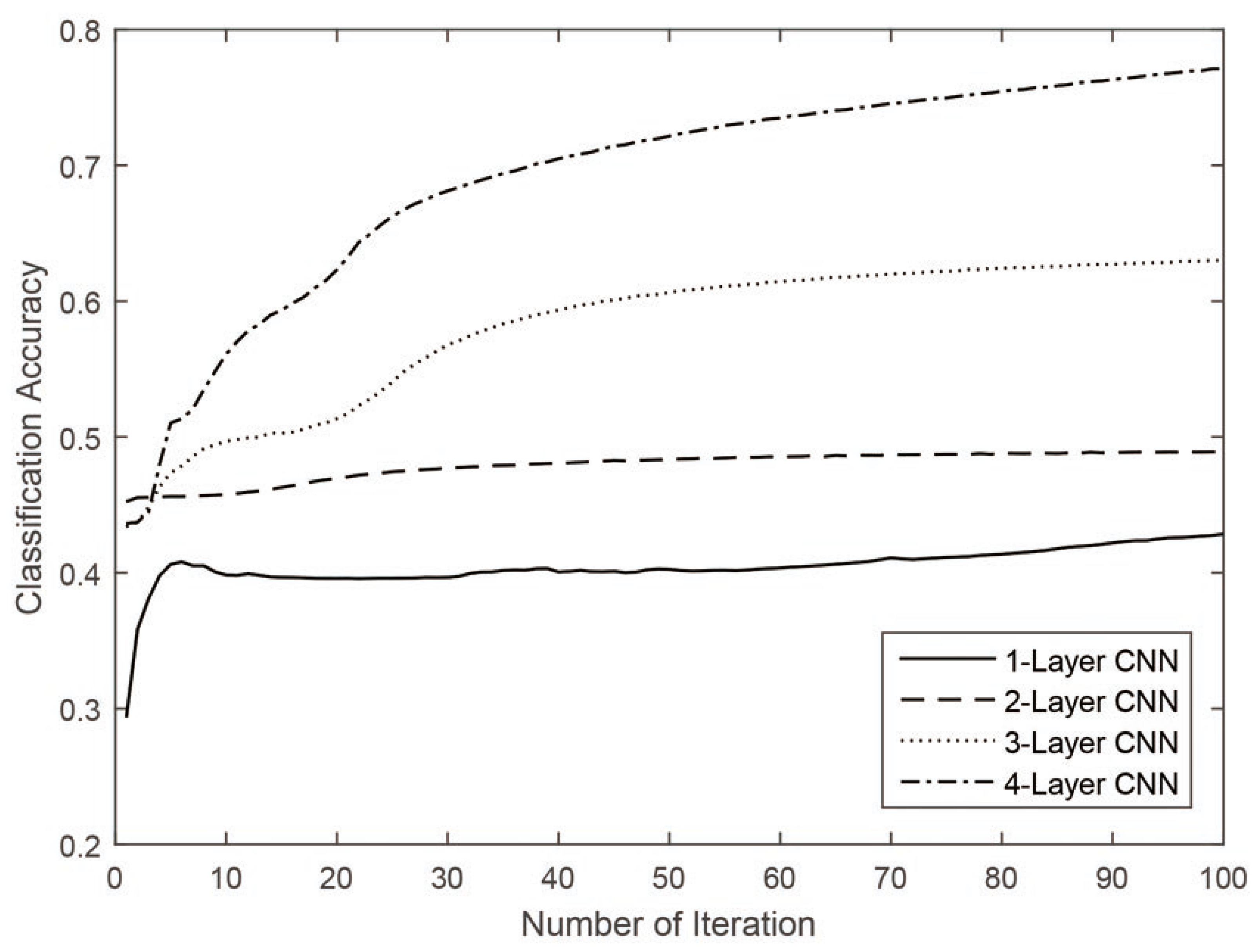
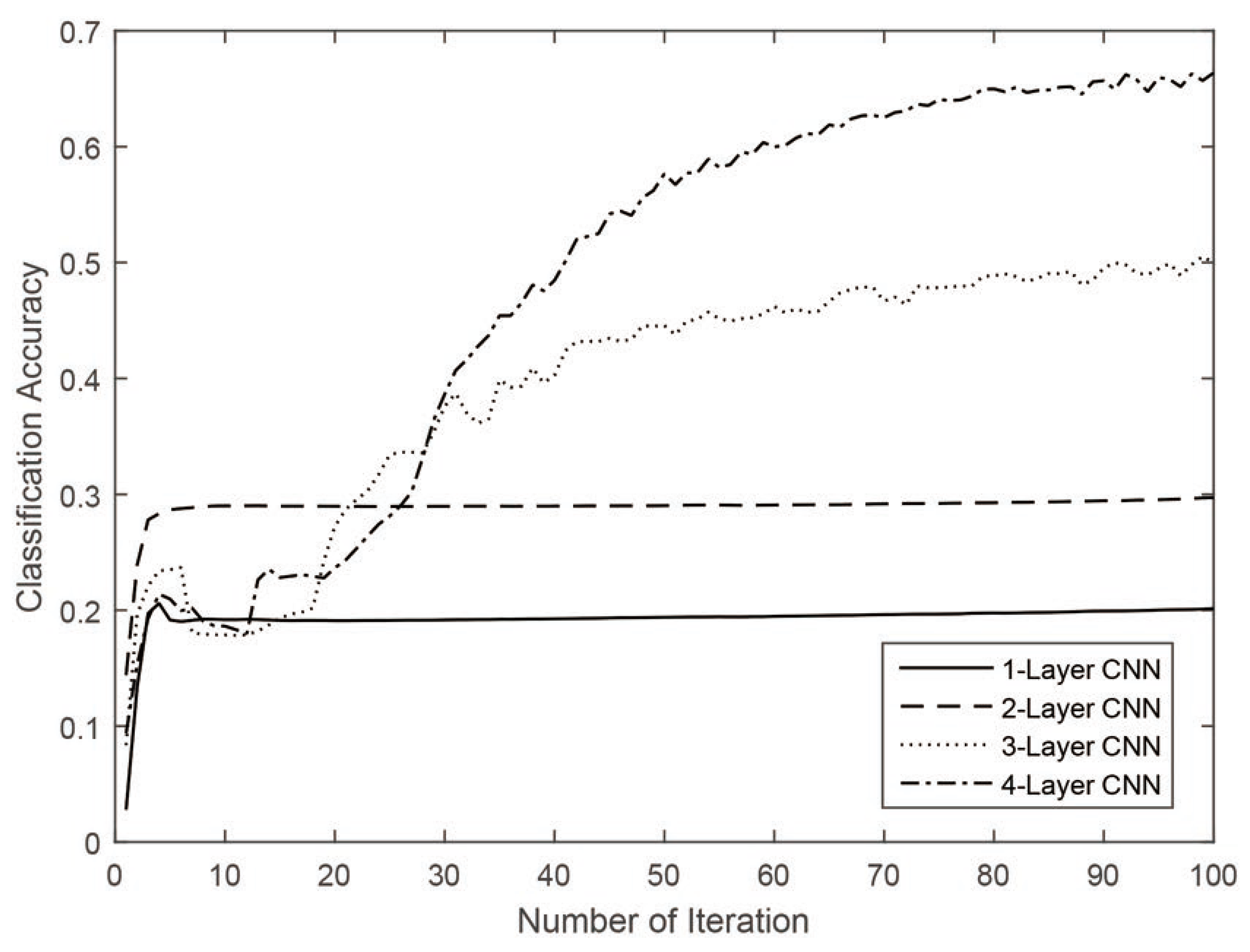
The depth parameter of CNN plays an important role in classification accuracy, because it controls the deep feature quality in terms of the level of abstraction. To measure the effectiveness of the depth parameter, a series of experiments were conducted on the Pavia University dataset. We set four different depths of CNNs from 1 to 4, and the feature number was fixed to 50. Overall accuracy was used to measure the classification performance with different depth configurations. The experimental results are shown in
Figure 4 and
Figure 5.
As can be seen from the figure, the classification accuracies can be obtained as increased with the increase in the depth configuration. The shallow layers contain low-level spatial features, but they vary greatly because of the constrained representation power. However, in deeper layers, the deep features are more robust and representative than those of lower ones. In addition, the shallow CNNs seem to have suffered more from overfitting, as presented in
Figure 5.
Figure 4.
Overall accuracies of the university of Pavia dataset classified by CNN under different depths.
Figure 4.
Overall accuracies of the university of Pavia dataset classified by CNN under different depths.
Figure 5.
Overall accuracies of Indian Pines dataset classified by CNN under different depths.
Figure 5.
Overall accuracies of Indian Pines dataset classified by CNN under different depths.
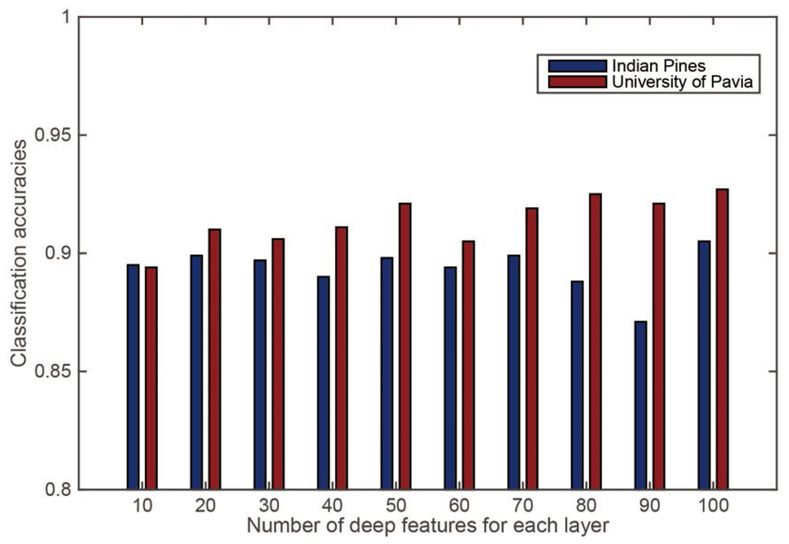
2.4.2. CNN Feature Number Effect
In the CNN framework, the number of features can determine the dimensionality of the extracted spatial features. To measure the effect of spatial number on classification accuracy, a series of experiments were conducted. The feature number was varied from 10 to 100, and the whole CNN framework was constructed with a four-layer structure. Overall accuracy was used to measure the performance of the CNN-based classification algorithm. The classification results are reported in
Figure 6.
Figure 6.
Classification results by setting different deep feature numbers for the CNN framework.
Figure 6.
Classification results by setting different deep feature numbers for the CNN framework.
From the results for the University scene, it can be seen that the classification accuracy increased with the increase in feature number. However, no appreciable change in accuracy was noticed beyond the number of 50 deep features. A similar pattern can be seen in the Indian Pines dataset as well. Unlike in the University scene, the classification accuracy in the Indian Pines data dropped significantly after 50, reaching the lowest point at 90. This indicates that the classification accuracy becomes unstable when the number of deep features increases beyond a limit. Therefore, for our experiments, we set the number of deep features to 50.
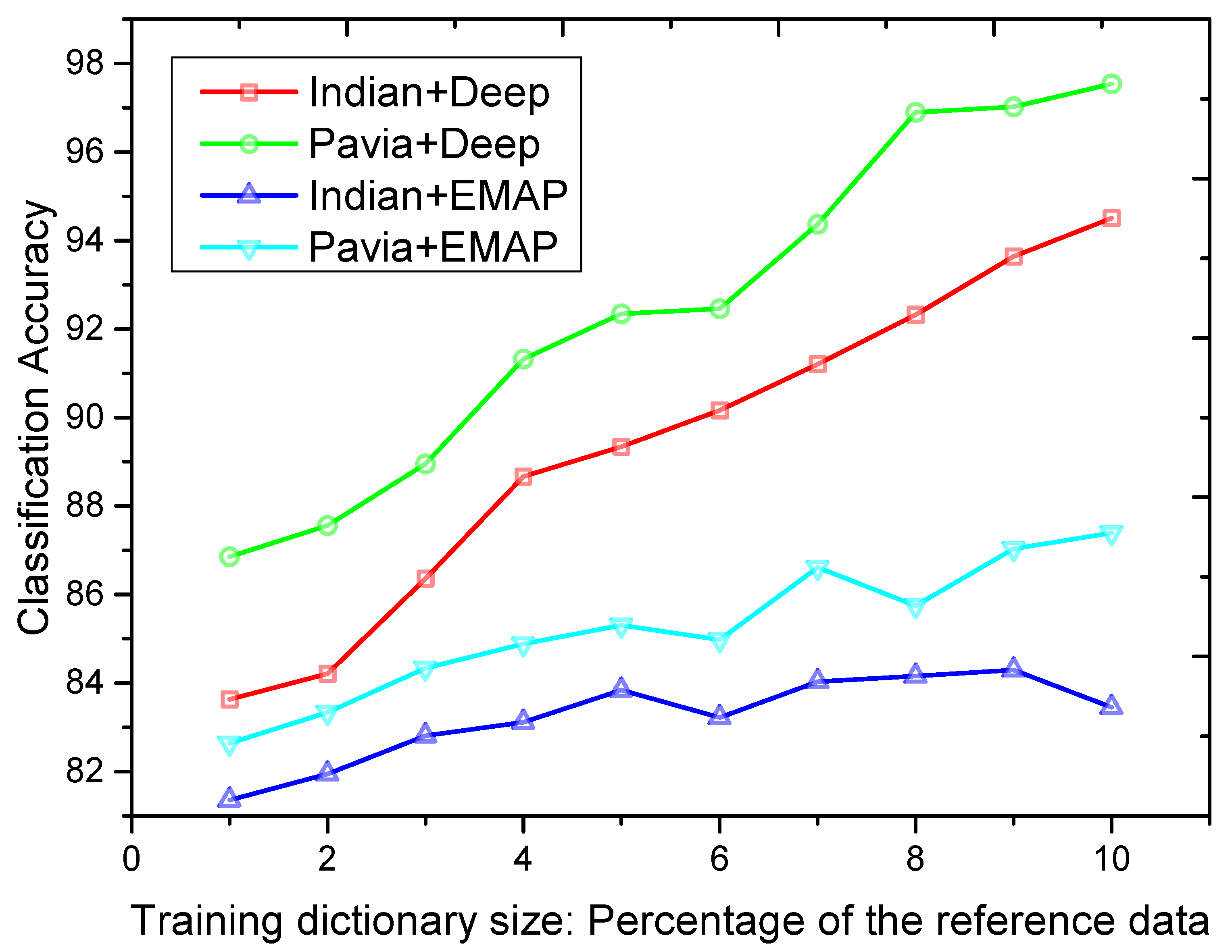
2.5. Analysis of Sparse Representation
To conclude the effectiveness of sparse representation, we analyzed the relationship between the size of the training dictionary in both EMAP space and the deep feature space and the classification accuracies obtained by the OMP algorithm in this work. In
Figure 7, the obtained classification accuracies are plotted as a function of the size of the training dictionary. The best classification accuracies are obtained by exploring the sparse representation of deep features for both the Indian Pines and Pavia University datasets. Generally, as the number of training samples increase, the uncertainty of classes decreases.
Figure 7.
Classification OAs as a function of training dictionary size (expressed as a percentage of training samples for each class) for the Indian Pines and Pavia University datasets.
Figure 7.
Classification OAs as a function of training dictionary size (expressed as a percentage of training samples for each class) for the Indian Pines and Pavia University datasets.
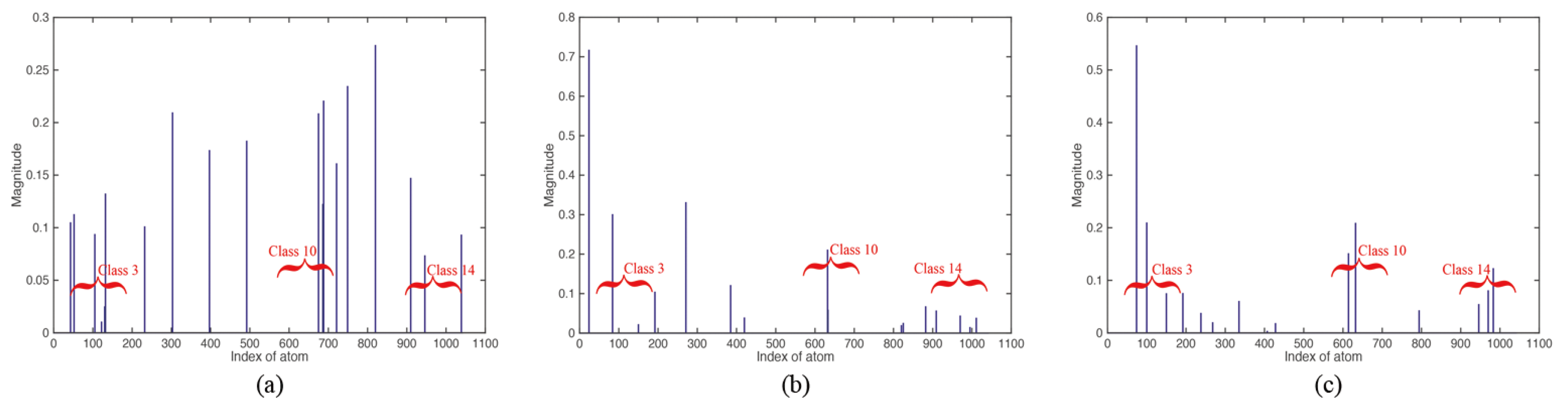
The following experiments illustrate the advantage of using a sparse representation in deep feature space for image classification over using the EMAP-based sparse coding. We considered a training dictionary made up of 1043 atoms and labeled the remaining samples as the test set. After constructing the dictionary, we randomly selected a pixel (belonging to Class 3) for sparse representation analysis, and the sparse coefficients are shown as bars in
Figure 8. From these figures, it can seen that in the original spectral space, the sparse coefficients appear so mixed up that it is hard to distinguish one class from the other. In the EMAP space, the differences between classes are becoming clear, but they are also hard to classify in the highly mixed-up pixel. In the deep feature space, the unknown pixel can be seen as belonging to Class 3, because it is more discriminative than that in the spectral or EMAP space. The reason behind this phenomenon is that the redundancy in spectral information and EMAP features greatly reduced the representativeness of the pixels. However, in the space of deep features, the correlation between different features is rather poor, and thus, it is more discriminative than the spectral and EMAP space.
Figure 8.
Estimated sparse coefficients (spectral space) for one pixel (belonging to Class 3) in the Indian Pines image. (a) Spectral space; (b) extended morphological attribute profile (EMAP) space; (c) deep feature space.
Figure 8.
Estimated sparse coefficients (spectral space) for one pixel (belonging to Class 3) in the Indian Pines image. (a) Spectral space; (b) extended morphological attribute profile (EMAP) space; (c) deep feature space.
2.6. Comparison of Different Methods
The main purpose of the experiments with such remote sensing datasets is to compare the performances of different state-of-the-art algorithms in terms of classification results. Prior to feature extraction and classification, all of the datasets were whitened with the PCA algorithm, preserving the first several bands that contained more than information.
To assess the effect of deep features, the well-known spatial feature extended morphological attribute profiles (EMAP) were introduced to classify the images in the spatial domain. Specifically, the EMAPs were built by using the attributes of area and standard deviation. Following the work in [
34], threshold values were chosen for the area in the range of {50,500} with a stepwise increment of 50 and for a standard deviation in the range of 2.5% to 20% with a stepwise increment of 2.5%. However, both EMAP and deep features are commonly shown in great redundancy and also with high dimensionality. To address the importance of the sparsity constraint in such spectral and spatial features, we added the original spectral information to our EMAP and deep feature-based sparse representation classification experiments. It should be noted that, in all of the experiments, the OMP algorithm was used to approximately solve the sparse problem for the original spectral information, EMAP and deep features, which can be denoted respectively as
,
and
. We also compared the proposed method with the nonlocal weighting sparse representation (NLW-SR) and the spectral-spatial deep convolutional neural network (SSDCNN) [
25] in terms of classification accuracy.
In addition, we compared the sparse-based classification accuracy of OMP with the accuracies obtained by several state-of-the-art methods. Recently, some novel classification strategies have proposed for classifying hyperspectral images, such as random forest [
35]. However, to evaluate the robustness of the deep features, the widely-used SVM classifier is considered as the benchmark in the experiment. It should be noted that the parameters of SVM were determined by five-fold cross-validation, and we selected the polynomial kernel for the rest of the experiments. The polynomial kernel can easily reveal the effectiveness of deep features, for future comparison. We denote the SVM-based classifications of spectral information, EMAP and deep features respectively as
,
and
.
For our research, a series of experiments were conducted to extract deep features with different numbers of feature map settings. Furthermore, the training dictionary was constituted of randomly-selected samples from a reference map. The remaining samples were used for evaluating the classification performances. Overall accuracy (OA), average accuracy (AA) and the Kappa coefficient were used to quantitatively measure the performance of the proposed method. The classification results are shown in
Figure 9 and
Figure 10.
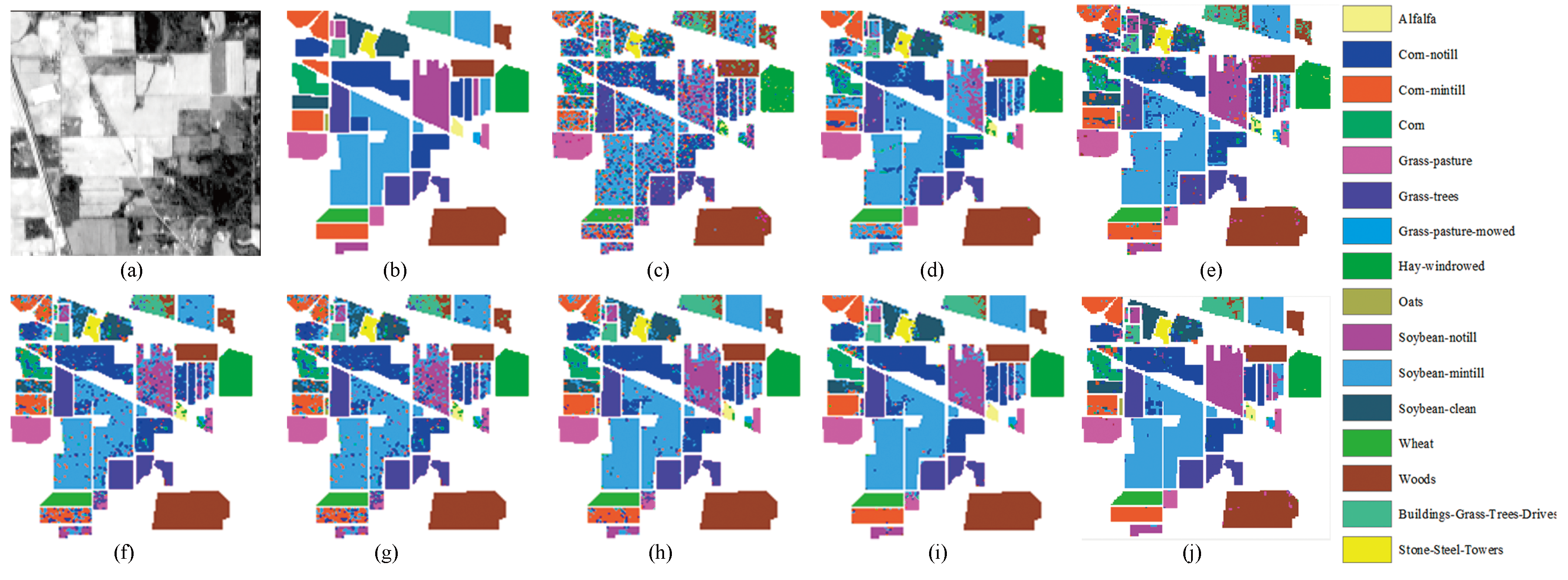
Figure 9.
Classification results obtained by different classifiers for the AVIRIS Indian Pines scene. (a) Original map; (b) Reference map; (c) Spe classification map; (d) EMAP classification map; (e) Deep classification map; (f) Spe classification map; (g) EMAP classification map; (h) Nonlocal weighting sparse representation (NLW-SR) classification map; (i) Spectral-spatial deep convolutional neural network (SSDCNN) classification map; (j) Deep classification map.
Figure 10.
Classification results obtained by different classifiers for the Reflective Optics System Imaging Spectrometer (ROSIS) Pavia University Scene; (b) Reference map; (c) Spe classification map; (d) EMAP classification map; (e) Deep classification map; (f) Spe classification map; (g) EMAP classification map; (h) NLW-SR classification map; (i) SSDCNN classification map; (j) Deep classification map.
2.7. Experiments with the AVIRIS Indian Pines Scene
In our first experiment with AVIRIS Indian Pines dataset, we investigate the characteristic of CNN-based deep features. Specifically, we considered the four-layer CNN with 50 features at each layer as the default configurations for deep feature generation.
We compare the classification accuracies obtained for the Indian Pines dataset by the proposed method with those obtained by the other state-of-the-art classification methods. To illustrate the classification accuracies obtained with a limited number of training samples in a better way, the individual class accuracies obtained for the case of 10% training samples are presented in
Table 1. As can be seen in this table, in most cases, the proposed deep feature-based sparse classification (Deep
) method provided the best results, in terms of individual class accuracies, as compared to the results obtained by other methods. When only the spectral information is considered, it is difficult to classify the Indian Pines image, because of the spectral mixture phenomenon. However, by introducing spatial information (EMAP), higher classification accuracies can be obtained in comparison to the accuracies obtained with the methods using only spectral information.
Table 1.
OA, average accuracy (AA) and Kappa statistic obtained after executing 10 Monte Carlo runs for the AVIRIS Indian Pines data.
Table 1.
OA, average accuracy (AA) and Kappa statistic obtained after executing 10 Monte Carlo runs for the AVIRIS Indian Pines data.
| Class | Train | Test | Spe | EMAP | Deep | Spe | EMAP | NLW-SR | SSDCNN | Deep |
|---|
| 1 | 3 | 43 | 54.88 | 94.88 | 85.42 | 33.33 | 96.51 | 96.34 | 90.34 | 95.83 |
| 2 | 14 | 1414 | 42.63 | 68.06 | 87.67 | 52.24 | 72.23 | 95.30 | 95.18 | 96.08 |
| 3 | 8 | 822 | 29.53 | 60.22 | 74.40 | 32.66 | 66.34 | 93.50 | 95.03 | 95.46 |
| 4 | 3 | 234 | 17.65 | 35.73 | 89.52 | 32.38 | 51.92 | 87.88 | 93.52 | 97.28 |
| 5 | 5 | 478 | 57.51 | 74.10 | 87.25 | 71.58 | 74.29 | 95.70 | 93.92 | 98.01 |
| 6 | 7 | 723 | 81.02 | 91.59 | 98.98 | 83.63 | 88.73 | 99.31 | 99.71 | 99.80 |
| 7 | 3 | 25 | 86.04 | 95.02 | 56.52 | 21.73 | 98.00 | 56.40 | 96.12 | 97.06 |
| 8 | 5 | 473 | 62.37 | 94.52 | 99.35 | 93.18 | 99.98 | 99.86 | 94.61 | 99.77 |
| 9 | 3 | 17 | 70.59 | 85.88 | 33.33 | 5.56 | 97.06 | 50.55 | 96.34 | 99.55 |
| 10 | 10 | 962 | 39.73 | 75.60 | 71.52 | 36.28 | 83.37 | 92.68 | 90.36 | 93.66 |
| 11 | 25 | 2430 | 73.31 | 87.37 | 94.32 | 63.21 | 88.61 | 96.43 | 95.67 | 96.53 |
| 12 | 6 | 587 | 21.72 | 57.68 | 77.17 | 39.31 | 70.49 | 91.14 | 88.34 | 91.52 |
| 13 | 3 | 202 | 87.28 | 96.44 | 99.36 | 93.15 | 98.61 | 91.52 | 96.65 | 100 |
| 14 | 13 | 1252 | 84.03 | 97.32 | 99.92 | 93.81 | 95.67 | 99.63 | 98.36 | 99.91 |
| 15 | 4 | 382 | 17.38 | 65.16 | 79.53 | 42.69 | 75.68 | 89.97 | 95.13 | 97.91 |
| 16 | 3 | 90 | 70.67 | 86.89 | 95.31 | 85.88 | 95.11 | 98.09 | 97.84 | 98.29 |
| OA | 56.73 | 79.07 | 83.18 | 61.42 | 82.70 | 95.38 | 96.02 | 97.45 |
| AA | 56.04 | 79.17 | 88.83 | 55.04 | 84.54 | 89.64 | 93.59 | 95.91 |
| Kappa | 49.88 | 76.08 | 87.18 | 55.68 | 80.26 | 95.26 | 94.67 | 96.36 |
| time (s) | 2.13 | 13.26 | 86.32 | 31.32 | 40.23 | 35.36 | 124.32 | 92.61 |
As regards the sparse representation effects, some important observations can be made from the content of
Table 1. After introducing the sparse coding technique, both EMAP and deep feature-based classification methods show a significant improvement in terms of classification accuracy. This reveals the importance of using sparse representation techniques, particularly in EMAP and the deep feature space.
2.8. Experiments with the ROSIS Pavia University Scene
In the second experiment with the ROSIS Pavia University scene, we investigated the characteristic of CNN-based deep features. As in the case of the AVIRIS Indian Pines dataset, here also, we considered, for deep feature generation, a CNN with four layers and 50 features at each layer as the default configuration. Unlike the image of the Indian Pines dataset, the image of the Pavia University dataset is of high spatial resolution, which is even more complicated in terms of classification. Nine thematic land cover classes were identified in the university campus: trees, asphalt, bitumen, gravel, metal sheets, shadows, self-blocking bricks, meadows and bare soil. There are 42,776 reference datasets. From the training dataset, we randomly selected 300 samples per class to obtain the classification results by six different classification methods, and the results are presented in
Table 2. The table shows the OA, AA, Kappa and individual class accuracies obtained with different classification algorithms. It can be seen that the proposed classification method Deep
provided the best results in terms of OA, AA and most of individual class accuracies.
In comparison, the classification accuracies obtained by using the SVM classifier tend to be lower than those obtained by sparse coding-based methods. With the introduction of EMAP features, the classification accuracies increased significantly, indicating thereby that spatial features are important, especially for high spatial resolution images. However, great redundancy lies in the EMAP space. Therefore, sparse coding-based OMP can give better performance in terms of classification accuracy. Compared to EMAP features, deep features are more effective and representative. Therefore, deep feature-based classification methods (both Deep and Deep) provide higher classification accuracy.
Table 2.
OA, AA and Kappa statistic obtained after executing 10 Monte Carlo runs for the ROSIS Pavia University scene.
Table 2.
OA, AA and Kappa statistic obtained after executing 10 Monte Carlo runs for the ROSIS Pavia University scene.
| Class | Train | Test | Spe | EMAP | Deep | Spe | EMAP | NLW-SR | SSDCNN | Deep |
|---|
| 1 | 300 | 6631 | 84.87 | 86.96 | 96.78 | 65.66 | 89.31 | 90.25 | 84.56 | 94.78 |
| 2 | 300 | 18,649 | 64.53 | 78.99 | 97.83 | 60.38 | 84.74 | 97.13 | 98.95 | 99.29 |
| 3 | 300 | 2099 | 74.54 | 81.24 | 77.87 | 52.35 | 82.99 | 99.80 | 96.62 | 98.65 |
| 4 | 300 | 3064 | 94.37 | 95.02 | 87.74 | 92.57 | 76.92 | 97.42 | 95.33 | 97.53 |
| 5 | 300 | 1345 | 99.61 | 99.41 | 97.74 | 98.93 | 99.32 | 99.97 | 76.65 | 100 |
| 6 | 300 | 5029 | 72.77 | 84.98 | 81.48 | 47.89 | 88.62 | 99.50 | 98.45 | 99.91 |
| 7 | 300 | 1330 | 96.77 | 98.90 | 69.12 | 84.71 | 99.71 | 98.85 | 99.62 | 99.80 |
| 8 | 300 | 3682 | 77.59 | 90.88 | 86.92 | 74.59 | 87.88 | 98.24 | 94.57 | 99.09 |
| 9 | 300 | 947 | 99.44 | 99.21 | 99.89 | 96.19 | 92.08 | 86.70 | 96.83 | 98.29 |
| OA | 75.28 | 84.92 | 91.80 | 65.62 | 86.61 | 96.50 | 95.18 | 98.35 |
| AA | 84.94 | 90.62 | 88.39 | 74.81 | 89.06 | 96.43 | 93.51 | 98.61 |
| Kappa | 69.14 | 80.90 | 90.12 | 57.15 | 82.85 | 95.34 | 93.64 | 97.86 |
| time (s) | 2.51 | 34.92 | 93.19 | 86.82 | 97.63 | 57.31 | 134.75 | 104.82 |


