Article

Multitemporal Monitoring of Plant Area Index in the Valencia Rice District with PocketLAI

by
Manuel Campos-Taberner
1,*,
Franciso Javier García-Haro
1,
Roberto Confalonieri
2,
Beatriz Martínez
1,
Álvaro Moreno
1,
Sergio Sánchez-Ruiz
1,
María Amparo Gilabert
1,
Fernando Camacho
3,
Mirco Boschetti
4 and
Lorenzo Busetto
4
1
Department of Earth Physics and Thermodynamics, Faculty of Physics, Universitat de València, Dr. Moliner, Burjassot 46100, València, Spain
2
Department of Agricultural and Environmental Sciences-Production, Landscape, Agroenergy, Cassandra Lab, Università degli Studi di Milano, Via Celoria 2, 20133 Milan, Italy
3
EOLAB, Parc Científic Universitat de València, Catedrático A. Escardino, 46980 Paterna, Spain
4
Institute for Electromagnetic Sensing of the Environment, Italian National Research Council, Via Bassini 15, 20133 Milan, Italy
*
Author to whom correspondence should be addressed.
Remote Sens. 2016, 8(3), 202; https://doi.org/10.3390/rs8030202
Submission received: 14 December 2015 / Revised: 15 January 2016 / Accepted: 18 February 2016 / Published: 1 March 2016
(This article belongs to the Special Issue Remote Sensing in Precision Agriculture)

Abstract

:
Leaf area index (LAI) is a key biophysical parameter used to determine foliage cover and crop growth in environmental studies in order to assess crop yield. Frequently, plant canopy analyzers (LAI-2000) and digital cameras for hemispherical photography (DHP) are used for indirect effective plant area index (PAIeff) estimates. Nevertheless, these instruments are expensive and have the disadvantages of low portability and maintenance. Recently, a smartphone app called PocketLAI was presented and tested for acquiring PAIeff measurements. It was used during an entire rice season for indirect PAIeff estimations and for deriving reference high-resolution PAIeff maps. Ground PAIeff values acquired with PocketLAI, LAI-2000, and DHP were well correlated (R2 = 0.95, RMSE = 0.21 m2/m2 for Licor-2000, and R2 = 0.94, RMSE = 0.6 m2/m2 for DHP). Complementary data such as phenology and leaf chlorophyll content were acquired to complement seasonal rice plant information provided by PAIeff. High-resolution PAIeff maps, which can be used for the validation of remote sensing products, have been derived using a global transfer function (TF) made of several measuring dates and their associated satellite radiances.

Graphical Abstract

1. Introduction

With the aim of managing plant needs in a more efficient way, precision agriculture has arisen as a rush of technological enhancements to classical farm management tools [1,2]. Detailed geo-spatial information on plant and soil properties is essential knowledge in crop management. In this context, remote sensing has become a very efficient tool for precision farming of large areas through data acquired by sensors on-board satellite platforms [3], airborne imagery [4], and unmanned aerial vehicles (UAVs) [5]. In this framework, rice cultivation is one of the most extended land uses for food production worldwide and has therefore been the main objective of many studies using optical [6,7] and radar [8,9,10] remote sensing techniques. In this context, leaf area index (LAI) is a key biophysical variable for both crop monitoring and modelling applications, defined as the total one-sided leaf area in relation to the ground [11]. LAI has been used in agricultural and remote sensing studies [12,13], including precision agriculture [14], and is regarded as a key input in global models of ecosystem, hydrology, climate, ecology, biogeochemistry, and productivity [15].
In situ LAI measurement methods can be divided into two main categories: direct and indirect [16,17]. Direct methods require an effort in collecting an optimal sample size and estimating plant density, which involve destructive harvest techniques [18]. Direct and indirect methods are complementary, as direct LAI measurements can be used a reference or calibration for indirect measurements. Indirect methods allow the inference of LAI from observations of another variable. They are generally faster than direct methods and allow larger spatial sample collection. Indirect methods can be divided into indirect contact LAI measurements and indirect non-contact measurements [19]. Indirect contact LAI methods are based on the estimation of the contact frequency [20], while indirect non-contact methods are based on the estimation of the gap fraction [21]. Contact frequency is the probability that a beam (radiation) penetrates inside the canopy and interacts with the vegetation. On the other hand, gap fraction is the integrated value of the gap frequency, which accounts for the probability that the beam will have no contact with the vegetation until it reaches the ground. Sensors like LAI-2000 or LAI-2200 Plant Canopy Analyzers (LI-COR, Inc., Nebraska, USA) measure the gap fraction from five different angles simultaneously. Digital hemispherical photography (DHP) is another indirect technique for computing the gap fraction through cameras with hemispherical lenses (fish-eye) coupled.
This method estimates LAI from measurements of the gap fraction, defined as the fraction of sky seen from below the canopy (upwards photography) or fraction of soil seen from above (downwards photography). Both Plant Canopy Analyzers and DHP are some of the most widely used classical optical instruments for indirect LAI estimation [19,22]. Classical commercial instruments have proven to be a good alternative to destructive methods in many experimental conditions [23] but these instruments are usually quite expensive both to purchase and to maintain. Due to their weight and strict requirements concerning acquisition protocol, they can also prove to be quite difficult to use in cases in which access to the canopy or placement of the instrument either below or above the canopy is difficult, such as in the case of flooded rice fields. Specifically, DHP techniques requires high effort by the operator during the classification process needed to obtain a LAI estimate. This fact limits the deployment of these measurements in near real time applications. An additional drawback when using these instruments is the time needed for repairing them in case of damage. A delay in the repair or replacement of the instrument may lead to canceling the field campaign in the worst case.
Recently, in the context of exploiting the technology implemented in smartphones for studies dealing with natural sciences, we introduced a mobile application called PocketLAI for leaf area index estimation [24]. PocketLAI was already successfully tested against Decagon AccuPAR Ceptometer, and it was used to measure LAI both on rice and other crop types also deviating from ideal assumptions of the light transmittance model used [25]. Smartphones are becoming an accessible daily instrument for most of the population. The use of smartphone components such as global position system (GPS), camera, accelerometer, and core processing power makes them suitable for a number of purposes, including methods for indirect LAI estimation. Smartphone capabilities are growing day by day, making them a reliable alternative to classical measuring instruments.
Leaf area index estimates refer only to leaf elements of the plant. Destructive methods only allow for measurement of leafs [26], but when dealing with indirect methods, several important considerations should be taken into account for a proper definition of the measured variable. In particular, for in situ LAI acquisitions and remote sensing observations, if no distinction is made between leaves and other plant elements, the proper term to use is PAI (Plant Area Index) rather than LAI [27,28,29]. Canopies are made of green photosynthetically active elements and other elements which are not green and therefore non-photosynthetically active (senescent leaves, trunks, branches, fruits, and flowers). Hence, to represent the photosynthetic functionality of all elements of the plant, PAI should be corrected to GAI (Green Area Index) [30]. Nevertheless, a proper indirect determination of GAI requires optical instruments able to distinguish green from non-green elements within the canopy [19]. Since this study deals with measurements and estimates taking into account all elements of the rice plant during all phenological stages, the term PAI will be used throughout the manuscript.
Temporal information on crop status is a requirement for better crop monitoring used to support agronomical management. In this context, other crop parameters, such as leaf chlorophyll content (Chl) or plant phenological stages should be acquired in order to complete temporal information of the crop. The identification of phenological stages can be addressed by visual interpretation of the plant morphological characteristics. This procedure can be carried out following standardized protocols, such as the Biologische Bundesanstalt Bundessortenamt and Chemical industry (BBCH) [31], which provides a description of the major morphological characteristics of each plant development stage assigning a specific numerical code for each one. An example of using the BBCH scale to identify phenological stages over rice fields can be found in [32]. On the other hand, chlorophyll content provides information about the physiological status of plants, nutrient stress, photosynthesis, and growing periods [33,34]. Chlorophyll concentration may change throughout different stages of plant phenology and is affected when crop plants are under stress conditions, mainly due to changes in soil nitrogen content [35]. Thus, leaf chlorophyll content becomes a key issue for agronomists and farmers to make management decisions at critical stages and has been widely studied by the remote sensing community [36,37,38]. Direct field measurements of chlorophyll content over large areas require a big effort in collecting destructive samples and conducting laboratory chemistry methods. Conversely, the use of handheld devices, such as SPAD-502 (Minolta Osaka Company, Ltd., Japan), are being used for rapid non-destructive sampling of leaf chlorophyll content [36,39]. For these purposes, continuous seasonal field phenology and leaf chlorophyll content were measured to complement seasonal rice plant information provided by PAI acquisitions.
In situ bio-physical parameters acquired during field campaigns are usually used for the validation of coarse satellite-derived products [40,41,42]. For these purposes, field measurements must follow several good practices and protocols [43]. Validation is commonly addressed through the derivation of a reference high-resolution map of an area covering several moderate resolution pixels [44,45]. The broadest strategy for the validation of satellite products is based on a bottom-up approach: it starts from the scale of the individual measurements that are aggregated over an elementary sampling unit area (ESU) corresponding to a support area consistent with that of the high-resolution imagery used for the up-scaling of ground data [44,46].
The main aim of this study is to monitor the rice plant area index with PocketLAI, assessing its consistency and performance with LAI-2000 and DHP during an entire rice season. The analysis of PocketLAI performance includes inter-comparison of field measurements and derived (upscaled) maps, which can be used for continuous monitoring and validation of LAI products. This study contributes to instrument comparison studies of rice.
The remainder of this study is organized as follows: Section 2 describes the study area and the sampling strategy outlining the in situ PAI measurements and describing the instruments used. Section 3 discusses the obtained results and the ancillary bio-physical variables used for rice monitoring, and finally Section 4 concludes the paper with a discussion and outline of the future research.

2. Materials and Methods

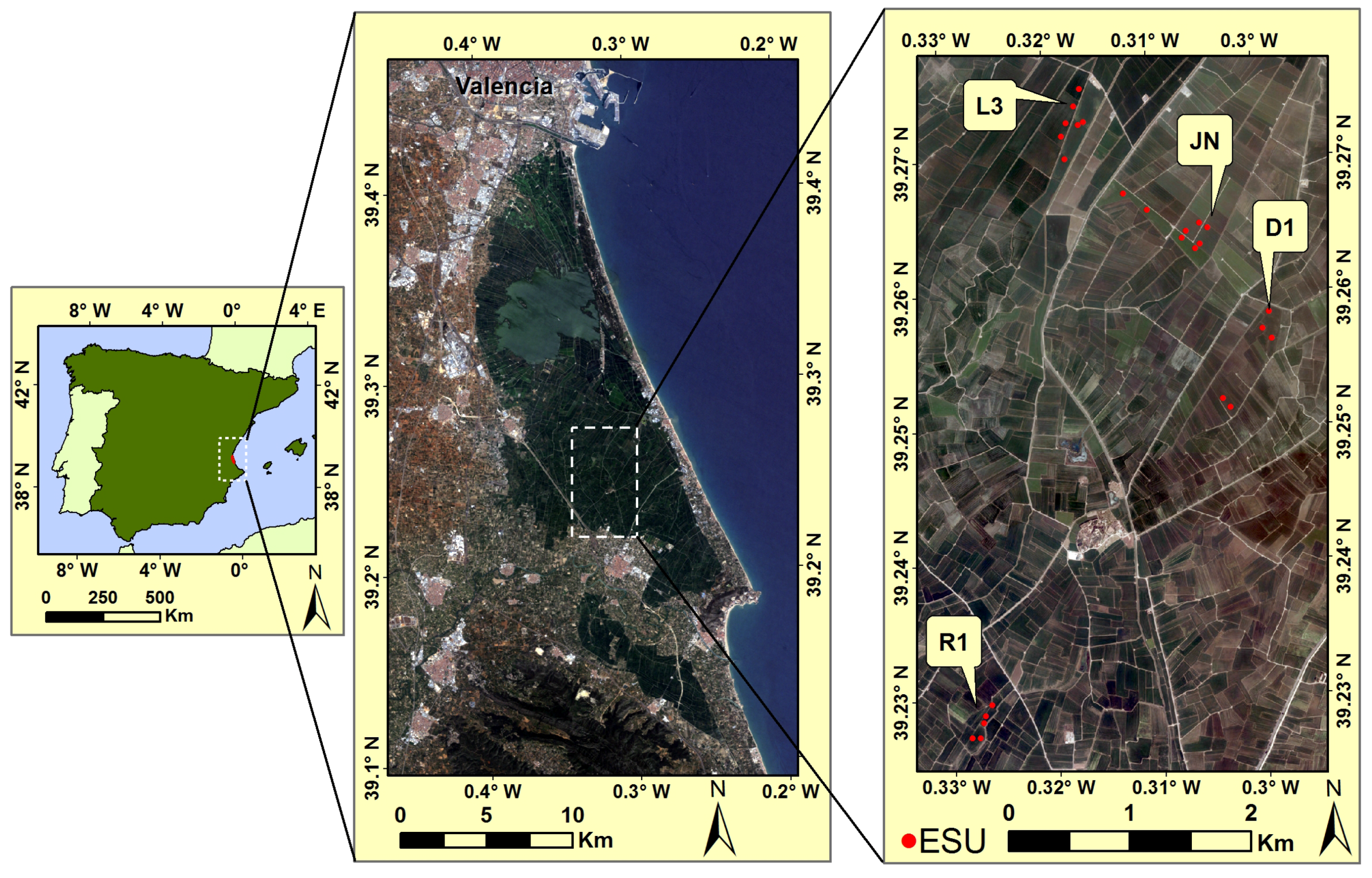
2.1. Study Area and Field Campaign

The study area is located in selected farms of the rice district of Sueca (39°16’N, 0°18’W), situated in the south of Valencia, in Eastern Spain (see Figure 1). The area has a typical Mediterranean climate; mild, with an average annual humidity of 65%. The average annual temperature is 17 °C. Their mean values range from 11 °C in January, and 27 °C in August. The mean annual precipitation is approximately 430 mm, tending to be intense and concentrated in autumn.
The site is a homogeneous rice planting area of approximately 10 km × 20 km extension. Most of the paddy rice fields are rectangular and flat, approximately 100 m × 200 m. The rice cropping practices are common in the entire rice district. The sowing dates are around early May. The maturity stage is reached in early September, and the rice harvest begins in mid-September. Fields are flooded most of the time during the season. The two main rice varieties are Senia and Bomba, and are under the guarantee granted by the Regulatory Board of Designation of Origin Arròs de València http://www.arrozdevalencia.org. These rice varieties have different morphological structures. The Senia variety has more stacked up stems and leafs, while the Bomba variety has a considerably greater height.
ERMES (an Earth obseRvation Model based ricE information Service) http://www.ermes-fp7space.eu/ is an FP7 Project funded by the European Commission with the objective of developing a prototype of downstream service dedicated to the rice sector to support authorities and farmers. In the framework of ERMES, ground measurements of phenology, plant height, chlorophyll content, FAPAR (Fraction of Absorbed Photosynthetically Active Radiation), and PAI were acquired on 26 ESUs from June the 17th to September the 8th in 2014. Measurement dates were selected to cover the entire rice season.

2.2. Spatial Sampling Strategy

The sampling strategy is a critical issue and should include considerations such as the number, dimensions, and spatial distributions of ESUs, driven by the heterogeneity of the study area, and the sampling scheme within each individual ESU. The 26 ESUs were selected within homogeneous rice fields. The fields were selected in order to take into account the main cultivated rice varieties. A reliable sampling covering the maximum bio-physical parameter variability was done. Over each ESU, the same sampling scheme was used as recommended by the VALERI (Validation of Land European Remote sensing Instruments) protocol in the case of row crops. This protocol suggests to take measurements along small transects between rows and incorporate some random acquisitions to prevent possible biases in the characterization of the row effect. ESUs were located at least 30 m away from the field borders and were approximately 20 m × 20 m in size. In order to characterize the variability within each ESU, a range of 18 to 24 measurements of the bio-physical variables were taken. This number of replicates allows to obtain a statistically significant mean estimate of each bio-physical variable per ESU. The center of the ESU was geo-referenced using GPS for later matching and association of the mean of each bio-physical variable with the reflectance derived from satellite data.

2.3. Effective Plant Area Index (PAIeff)
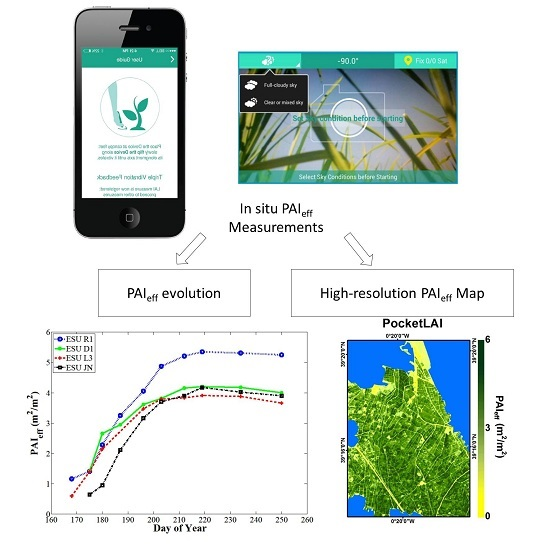
Strictly speaking, the “true LAI” can be measured only using a planimeter [26]. Indirect methods compute an effective leaf area index through the following relation:
L A I e f f = · L A I
where Ω is the aggregation or dispersion parameter [47,48], also known as the clumping index [11]. It accounts for canopy structure, geometry and foliage clumping. PocketLAI, LAI-2000, and DHP actually provide an estimate of the plant area index, since all parts of the plant contribute to the canopy transmittance. Indirect methods based on gap fraction measurements do not have the ability to determine if some leaves are present behind the stems, branches, flowers, or trunk [29]. In this study, we are using PAIeff, since we are considering the rice fields as a turbid medium (minimum clumping).

2.4. PocketLAI

In this study, we proposed the use of PocketLAI for in situ non-destructive rice PAIeff monitoring. PocketLAI is a smartphone application based on the segmentation of images acquired at 57.5° below the canopy to estimate the gap fraction [24]. It is based on a simplified model of light transmittance under the assumption of a random spatial distribution of infinitely small leaves. In this case, the gap fraction P 0 ( θ v , ϕ v ) in the zenith angle θ v direction and azimuth angle ϕ v is given by:
P 0 ( θ v , ϕ v ) = exp G ( θ v ϕ v ) P A I cos θ v
where G ( θ v , ϕ v ) is the projection function, which can be considered as almost independent of leaf inclination (G ≊ 0.5) for a viewing angle of 57.5° (≊1 radian) [17]. Inverting Equation (2), PAI can be estimated from the gap fraction at this particular direction as follows:
P A I ( 57.5 ° ) = ln P 0 ( 57.5 ° ) 0.93 .
At this directional configuration, the information acquired is independent from leaf angle distribution and minimizes leaf clumping effects [30]. This property comes from the projection function used to compute gap fraction corresponding to the projection of a PAI unit into a given direction. This mobile application has been shown to perform well in canopies with different structures [25] and has proven its reliability in terms of both trueness and precision [24]. PocketLAI computes the gap fraction using the smartphone’s accelerometer and camera. The operator holds the device vertically below the canopy and rotates the device along its main axis. When the angle between the vertical and the normal to the screen reaches 57.5°, a camera frame is captured and processed using an algorithm based on a segmentation strategy to detect sky pixels. In this study, the smartphone was placed 5 cm above the shallow water. PockeLAI allows the averaging of various numbers of PAI estimates in order to get a representative measure of the ESU based on the visual jackknife method [18]. In this work, the mobile application was installed on a Samsung Galaxy S4 GT-I9505, with a Quad-Core 1.9 GHz processor and 2 GB RAM. The smartphone’s camera allowed PocketLAI to take images with a resolution of 4128 × 3096 pixels. With the aim of obtaining a representative measurement of each ESU, eighteen measurements acquired under similar illumination conditions were computed for each ESU following the strategy described in Section 2.2.

2.5. Digital Hemispherical Photography (DHP)

Digital hemispherical photography allows the computation of PAI measuring the gap fraction. The digital photographs were taken downward-looking and the distance between the camera and the top of the rice canopy was set to about to 1 m to avoid the case that leaves were too close to the lens. Although upward photography is easy for gap identification, it may overestimate the gap fractions and consequently underestimate the PAIeff in the case of rice [29]. Thus, in this study, given this underestimation and the characteristics of the rice plant (low height) and soil conditions (flooded), the downward-looking method was selected. During the ERMES field campaign, 16 photographs per ESU were acquired with the DHP and were subsequently processed using the Can-Eye software developed at INRA-CSE Avignon in order to meet the requirements of VALERI. Can-Eye computes effective PAI from gap fractions after an interactive thresholding classification process separating rice foliage from the background (downward view). The images were masked limiting to 60° zenith angle the valid range of fisheye lens to avoid edge distortions and ensuring that the area captured was within the ESU. Hemispherical photographs were taken maintaining the camera in an approximately horizontal position not-exceeding 10°, which is considered the threshold for minimizing errors due horizontal camera levelling in estimating PAI [28]. Photographs with suboptimal horizontal acquisition were excluded. A NIKON Coolpix5000 camera was used at the finest image resolution available (JPEG format at 2560 × 1920 pixels resolution) and a FC-E8 Nikon fisheye lens with a field of view of 183°. The camera with the fisheye lens was calibrated before the field according to the CAN EYE manual [49]. The PAIeff was computed using the Miller’s formula [50] as follows:
P A I e f f = 2 0 π / 2 ln P 0 ( θ ) cos ( θ ) sin ( θ ) d θ
In addition, the Can-Eye software proposes an estimate of the PAIeff derived from the gap fraction measured for a view angle of 57.5° in the same way that is computed in Equation (3). Can-Eye software simultaneously processes up to 16 images acquired over the same ESU. All images belonging to the same ESU were acquired with similar illumination conditions to limit the variation of color dynamics between images.

2.6. LAI-2000 Plant Canopy Analyzer

Li-Cor LAI-2000 was used to estimate the rice PAI using a gap fraction method that determines the PAI from measurements made above and below the canopy, which are used to determine canopy light interception at five zenith angles (7°, 23°, 38°, 53°, and 68°). Canopy transmission is measured between 320 and 490 nm. LAI-2000 computes the PAIeff using the Miller’s formula as:
P A I e f f = 2 0 π / 2 ln P ( θ ) ¯ cos ( θ ) sin ( θ ) d θ = 2 i = 1 5 K i ¯ W i
where Ki and Wi are the contact number and the weighting factor, and the subscript i refers to the number of the ring. P ( θ ) ¯ is the average probability of light penetration into the canopy, and the gap fraction Gi(θ) is computed as:
G i ( θ ) = exp ( ln P ( θ ) ¯ ) = exp ( 1 N ) j = 1 N ln ( B j A j )
The subscript j is number of readings (j = 1 ⋯ N), and Bj and Aj are the corresponding readings to below and above the canopy, respectively.
In this field campaign, a 270° view cap was used to limit the azimuthal field of view, facing away from the operator. Three replications of one measurement above and eight below the canopy were made for each measurement. Regarding below canopy measurements, the Li-Cor LAI-2000 instrument was placed about 5 cm above the shallow water. Measurements were made under diffuse light conditions in order to avoid incoming radiation from sunlit foliage.

2.7. Complementary Field Data

2.7.1. Phenology

The information regarding the phenology was obtained for all ESUs with in situ observations according to the BBCH scale for rice. Representative ESUs of the study area (see Figure 1) were selected in order to show phenology stages of the fields. The BBCH scale provides a continuous numerical range for identifying and describing the plant phenology. Table 1 describes the main rice stages as follows: stages 0 to 49 correspond to the vegetative phase of the rice cycle, stages 50 to 69 correspond to the reproductive phase, and stages 70 to 99 correspond to the maturation phase. The BBCH scale accounts for a single plant. If an operator aims to define the phenology stage of an ESU, at least half of the plants should present the same phenological state.

2.7.2. Chlorophyll Content

The leaf chlorophyll content has been obtained by means of a SPAD-502, which gives a leaf chlorophyll content estimate taking into account the radiation absorbed by leaves at specific wavelengths. SPAD-502 provides digital counts (DN) which are dimensionless and require an empirical calibration between SPAD-502 DN and extracted chlorophyll values in laboratory. This problem can be addressed using specific calibration curves, which includes linear, exponential, or polynomial calibration functions. In this work, a calibrated SPAD-502 using a power relationship to obtain leaf Chl content physical values in μg·cm−2 was used [36]. Hence, in order to characterize the chlorophyll content of the ESUs, 10–15 readings were made covering each ESU. SPAD-502 readings were made on the last completely unfolded leaf.

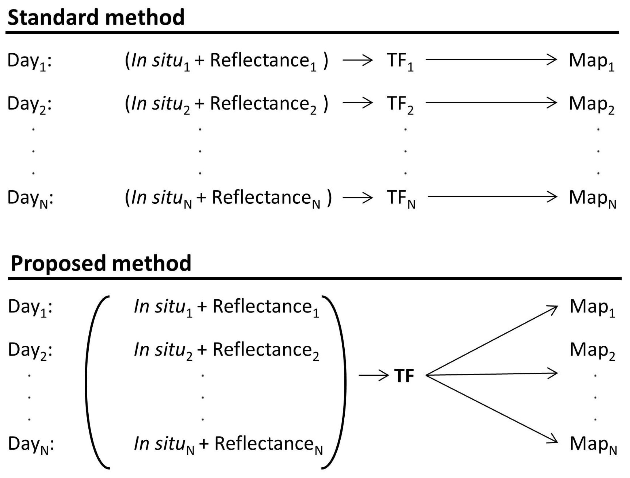
2.8. Transfer Function for High-Resolution PAIeff Mapping

In this study, the field measurements were also used for the derivation of a reference high-resolution map within the study area which can be used for remote sensing validation products. The derivation of high-resolution PAIeff maps is a procedure based on an empirical transfer function (TF) that establishes a relationship between the average PAIeff values from each ESU and the multispectral values from sensors onboard either satellite or airborne platforms. In this work, a relationship between the average PAIeff values from each ESU and radiometric values over concomitant Landsat-8 imagery in four spectral bands, namely green, red, near infrared, and shortwave infrared 1 bands (G, R, NIR, and SWIR1) was used. Following previous works [44] and recommendations [41,43,45], the up-scaling algorithm relies on a robust linear regression that evaluates the band combination that exhibits the lowest error. A multivariate ordinary least squares (OLS) regression is used, which assumes that the prediction Y (in situ PAIeff measurement) is related to the independent variable Xi, i = 1, 2, …, q (Landsat-8 radiometric values in the four selected bands) through the the following functional relationship:
Y j = β 0 + j = 1 q β j · X i j + ε ( i = 1 , , n )
where n is the number of observations, and βj are the parameters of the multiple linear regression. With the goal of minimizing the influence of outliers, an iteratively re-weighted least squares (IRLS) method is applied. This approach includes a weight factor to adjust the amount of each response value on the estimates provided by the model. ESUs with weights lower than 0.7 are usually linked either to samples located near the field borders or to experimental errors [44]. In order to evaluate the optimal Landsat-8 OLI band combination, we considered the weighted root mean square error (RW) and the cross-validation root mean square error (RC). The RW gives the mean prediction error assumed by the model for all the observations while the RC provides information about the model’s performance.
In this study, the response variable represents the three data sets of in situ PAIeff measurements (i.e., PAI e f f A P P , PAI e f f D H P , and PAI e f f L A I 2000 ), whereas the predictor variable is the radiometric information on the four Landsat-8 OLI spectral bands. Landsat 8 OLI images provide valuable information for crop monitoring at the local scale [51] due to the spatial (30 m) and temporal (16 day) resolutions. Images were downloaded as a Level 1T product and atmospherically corrected using the L8SR code, which corrects to surface reflectance from top of atmosphere (TOA) reflectance using ancillary NCEP (US National Centers for Environmental Prediction) water vapor data and TOMS (Total Ozone Mapping Spectrometer) ozone data sets. Landsat 8 OLI images were clipped to 1500 × 800 pixel size covering the entire rice area.
The standard method of generating a reference map relies on the information provided by spectral bands and vegetation indices from a single date of imagery [44,46]. This general method implies that each map is derived with a different TF made with the corresponding measurements and associated reflectances. One main feature of this work is the combination of field and satellite data from different acquisition dates in order to create a multitemporal data set which was used for building a unique global TF able to derive mutitemporal maps (see Figure 2).

3. Results

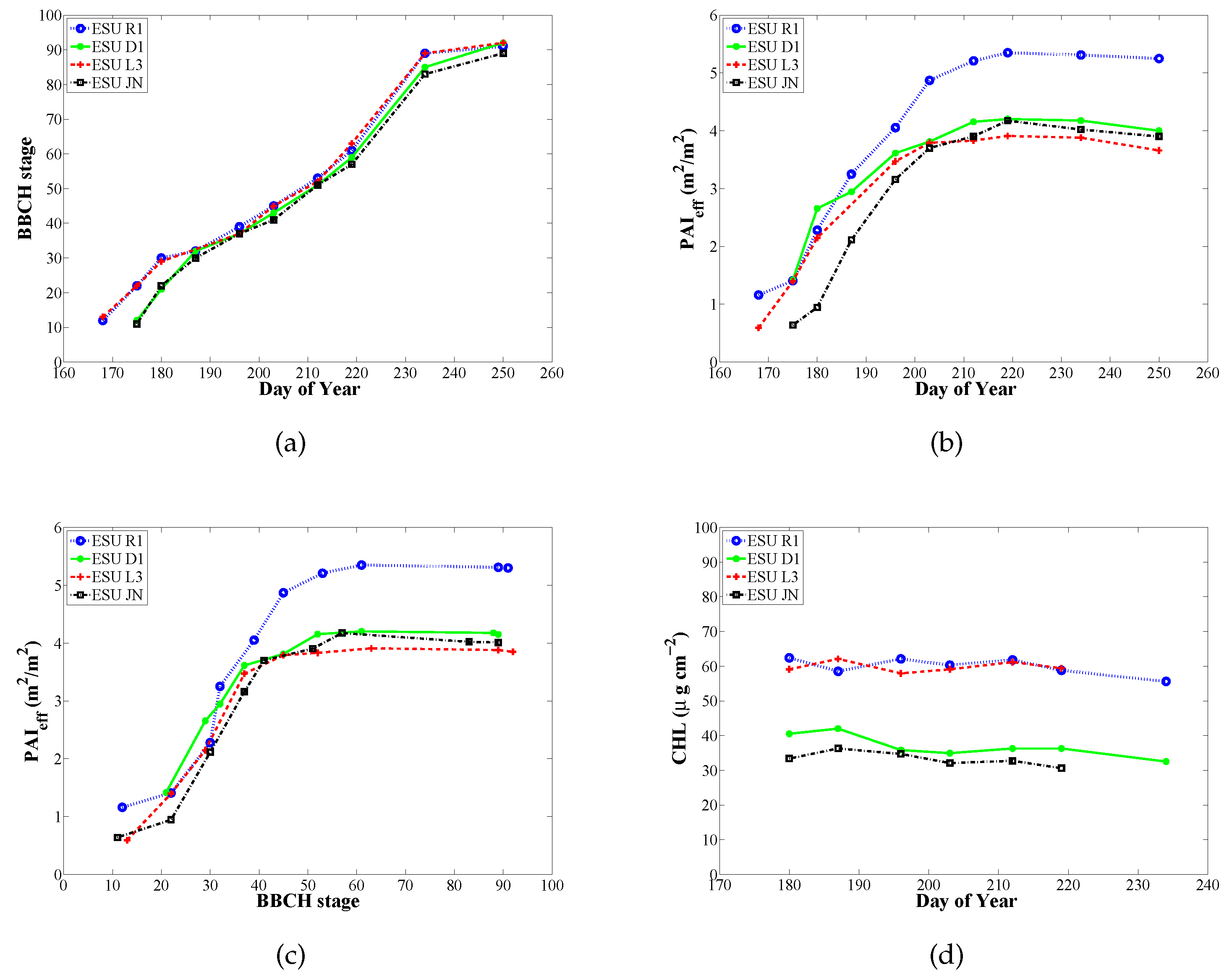
3.1. On the Temporal Evolution of the PAIeff Field Measurements

A general overview of the PAIeff measurements obtained during the field campaign shows that the range of PAIeff values obtained using all three instruments is according to the values reported in the literature for rice [29,52]. Seasonal variation of rice PAIeff (see Figure 3b) shows the typical behavior throughout the entire rice season. Maximum values of PAIeff were observed on day of year (DoY) 220. Significant differences in PAIeff time profiles were observed in the representative ESUs. Specifically, R1 clearly presented the highest values, about 1 m2/m2 at the beginning of the season and about 5.5 m2/m2 at almost the end of the growing season when the PAIeff values are maximum. R1 and L3 ESUs belong to same rice variety; nevertheless, a different PAIeff evolution was observed (see Figure 3b,c): plant density on R1 (number of rice plants per unit area) was significantly higher than on L3, leading to systematically higher PAIeff values.

3.2. On the Ancillary Data: Phenology and Leaf Chlorophyll Content

As part of the ERMES field campaign, phenology was monitored during 10 days from DoY = 168 to DoY = 251. In general, all representative ESUs have a similar behavior (see Figure 3a), since sowing dates were very similar in the study area. Comparison of rice PAIeff and BBCH seasonal variation (Figure 3c) highlights three most noticeable features: (1) the fast increase in PAIeff during the tillering and stem elongation vegetative stages (BBCH from 20 to 40); (2) the saturation of PAIeff during the stages of flowering, fruit development, and ripening (BBCH from 50 to 90), in which these vegetative and maturation phases the rice plant loses some leaves and becomes drier, PAIeff being practically constant; and (3) D1, JN, and L3 ESUs have a close evolution, while R1 shows higher PAIeff values due to higher plant density.
Rice leaf chlorophyll content measured with SPAD-502 showed a constant behavior during vegetative and reproductive stages, which means that no anomalies due to significant changes in Chl were found. A slight decrease in the rice Chl content was observed in the maturation stage due to the beginning of rice senescence (see Figure 3d). Since SPAD-502 readings were made in the last unfolded leaf, in most cases the estimated Chl content corresponded to leaves that were not senescent; i.e., on leaves where the hydrolytic processes that recycle nitrogen-rich compounds (including chlorophylls and rubisco) were not started yet. Consequently, although the total plant nitrogen content at the end of August were low (because of older leaves), measurements in the last-emitted leaf could still have high nitrogen content. This could explain why leaf chlorophyll contents were still high while the rice plants were approximately in the last part of the crop cycle. On the other hand, differences in leaf Chl values are related to the two main rice varieties of the study area. The Senia variety (R1 and L3 ESUs) presents leaves with a high chlorophyll content of about 60 μg·cm−2. By contrast, the Bomba variety (D1 and JN ESUs) presented lower chlorophyll content values, about 35–40 μg·cm−2. These Chl values explain the yellow greenish leaf color of the Bomba variety.

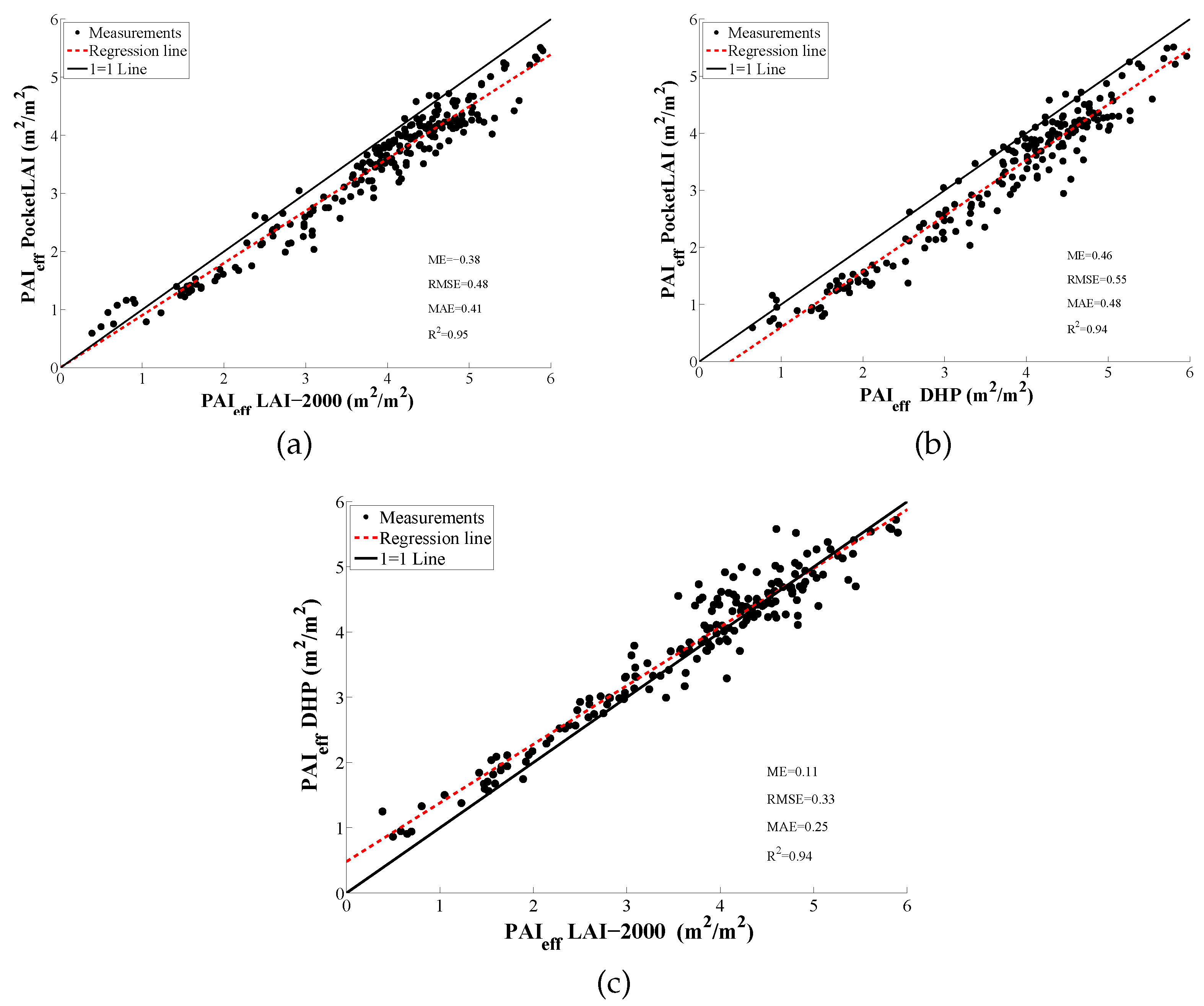
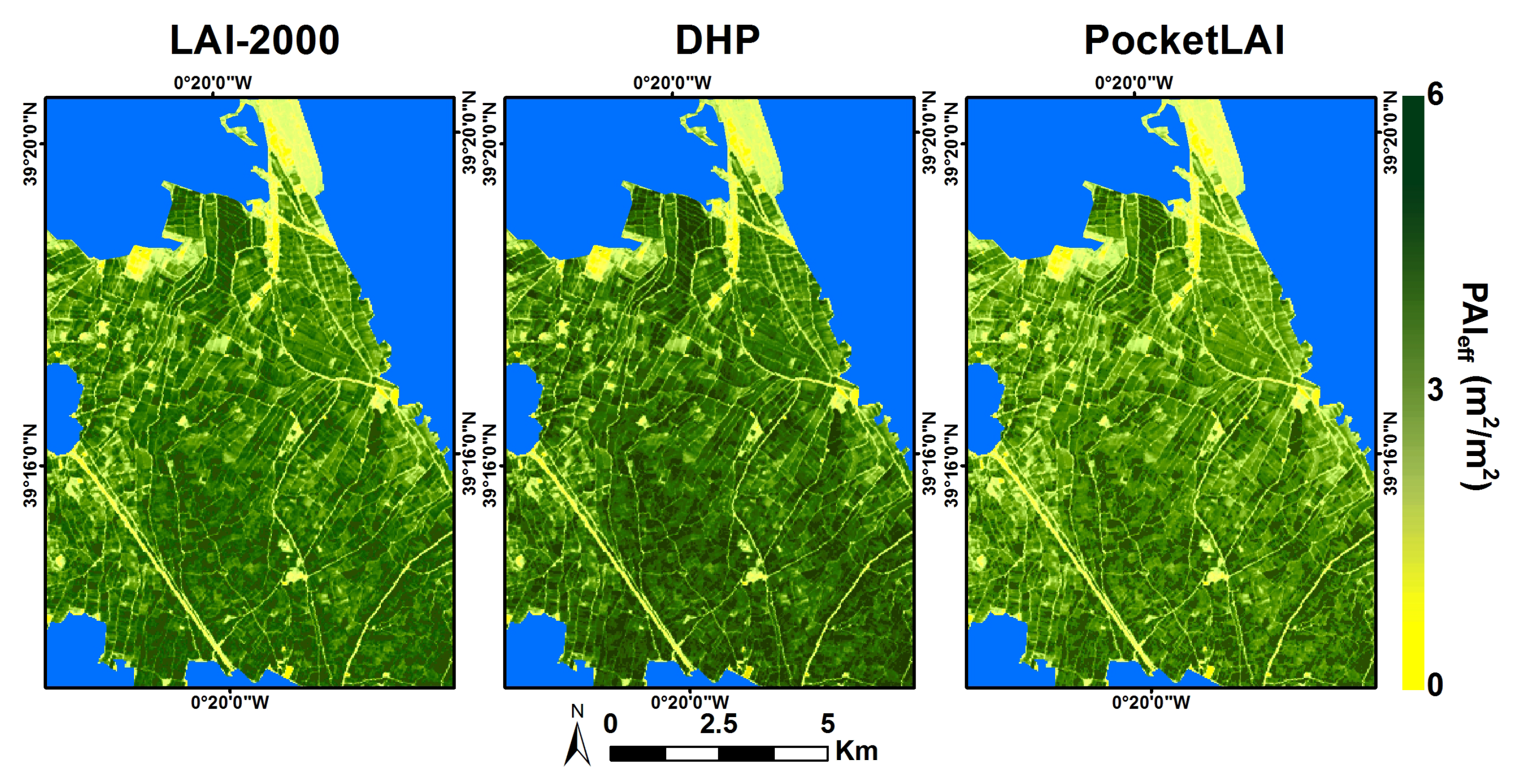
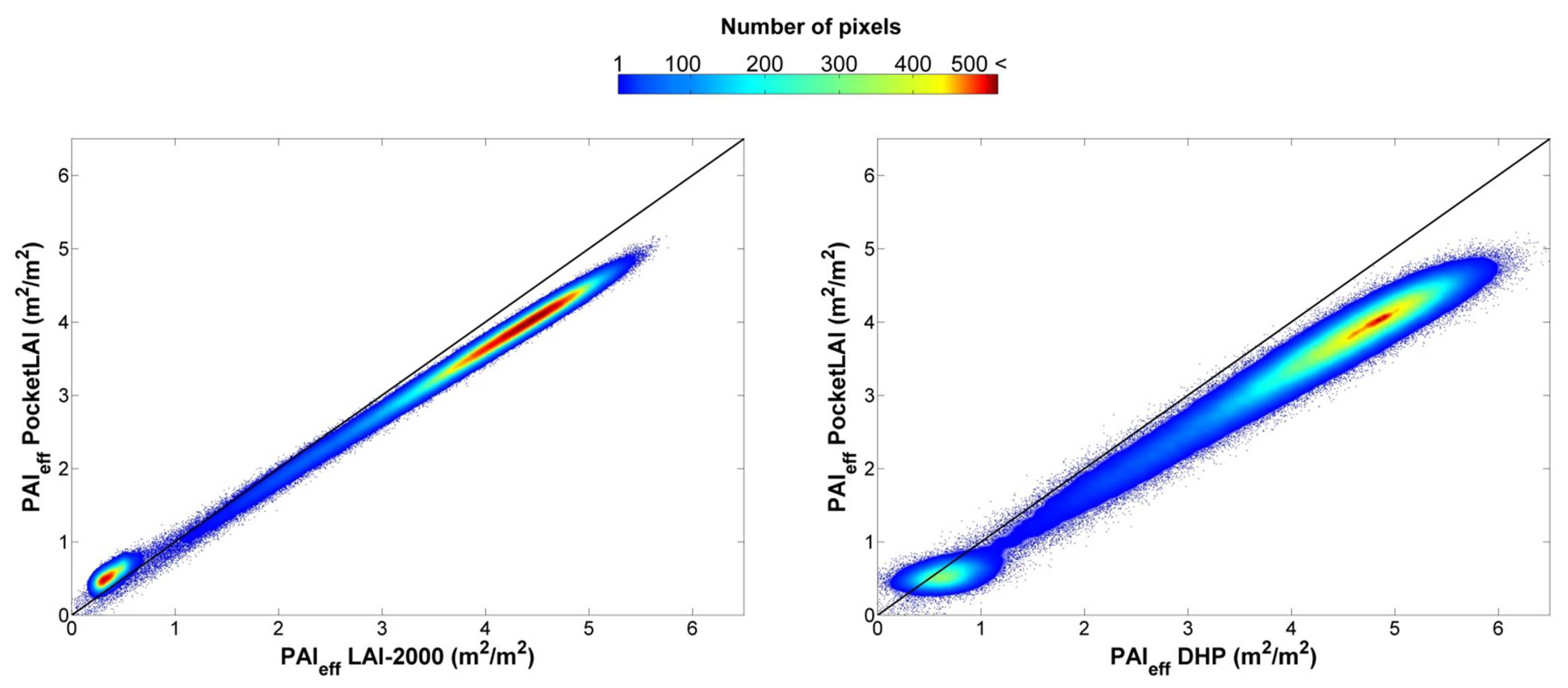
3.3. On the PAIeff Measuring Instruments and Maps Comparison

PocketLAI computes the PAIeff of an ESU, averaging each PAIeff calculated from each gap fraction reading on the ESU, while DHP and LAI-2000 first calculate the average gap fraction within an ESU and retrieve PAIeff from it. Since the gap fraction-PAIeff relationship is not linear, it is not equivalent to first average the gap fraction and then estimate the PAIeff than the contrary [17]. This fact may be one of the reasons why PocketLAI generally underestimates PAIeff values (see Figure 4). The PAIeff and PAIeff(57.5°) values obtained with DHP were used to compare estimates from LAI-2000 and PocketLAI with PAIeff, respectively. Different statistics were computed to assess the consistency and performance of the PocketLAI with LAI-2000 and DHP: root-mean-squared error (RMSE) and mean absolute error (MAE) were used to assess the accuracy, Mean error (ME) to evaluate the bias, and coefficient of determination (R2) to account for the goodness-of-fit and variability between instruments.
Effective PAI values computed with all three instruments are well correlated. The coefficient of determination computed between PAIeff estimates acquired with PocketLAI and classical instruments was R2 = 0.95 and R2 = 0.94 for LAI-2000 and DHP, respectively. Comparisons also reveal high accuracy and small bias between instruments (ME = −0.38 m2/m2, MAE = 0.41 m2/m2 for LAI-2000, and ME = 0.46 m2/m2, MAE = 0.48 m2/m2 for DHP). PocketLAI presents a very small negative bias regarding LAI-2000, although a slight positive bias is found at the beginning of the season (PAIeff < 1 m2/m2) (see Figure 4a). PocketLAI is also highly consistent with DHP, although it tends to produce slightly lower values (ME = 0.47) (see Figure 4b). Comparison between LAI-2000 and DHP instruments also shows good results in terms of accuracy, bias, and variability (RMSE = 0.33 m2/m2, ME = 0.11 m2/m2, R2 = 0.94 m2/m2) (see Figure 4c).
Indirect methods provide a PAIeff associated with several sources of measurement error, including performance of instruments, illumination conditions, simplification of leaf optical properties, suboptimal spatial sampling within an ESU, and saturation of optical signal in dense canopies. Specifically, variability observed when PAIeff values are greater than four typically correspond to rice plants in the reproductive phenology stage. At this point, there is a significant change in the rice morphological structure due to the panicle emergence, leading to an increasing variability of the estimates. Error, Bias, and correlation between instruments are small and do agree with previous studies in different crops [23,53] in which strong correlations (R2 = 0.96 and R2 = 0.94), small bias (ME ≈ 0.2) and accuracy (RMSE ≈ 0.5) were found.
These in situ PAIeff measurements allowed the creation of a transfer function, which was used to derive PAIeff maps. RW and RC errors in function of the selected Landsat-8 combination bands were computed for the TF. The best band combination was (SWIR1,NIR,R,G) in all three cases. This specific band combination reveals RW = 0.46 and RC = 0.50 in the case of PocketLAI, RW = 0.51 and RC = 0.52 in the case of LAI-2000, and RW = 0.50 and 0.51 in the case of DHP. Statistical indicators of the selected transfer functions showed good correlations and biases in all three cases (R2 > 0.93 and B < 0.02). For the shake of brevity we only show one derived PAIeff map per instrument, which corresponds to DoY = 196 and BCCH ≈ 35 (see Figure 5). The three derived maps show similar estimated PAIeff values within the study area. Nevertheless, the estimated PAI e f f A P P map shows a slight underestimation if it is compared with PAI e f f D H P - and PAI e f f L A I 2000 -derived maps. Pixels covering non-interest areas were masked out in blue color. Up-scaled maps derived from this ground dataset are made available for the validation of remote sensing products through the ImagineS www.fp7-imagines.eu (Implementing Multi-scale aGricultural Indicators Exploiting Sentinels) ground database.
Derived maps reveal PAIeff estimates fell within the expected range at that phenological rice state and show high consistency between classical instruments estimates. On the other hand, the map derived with PocketLAI measurements shows less intense greens, corresponding to values slightly lower than the ones retrieved either with DHP or LAI-2000. This fact is in agreement with the low PAIeff underestimation observed in the comparison of the in situ PAIeff measurements between the app and the classical instruments. All three estimated maps show expected within-field variations due to the spatial PAIeff variability of rice fields corresponding to different varieties, phenological stages, and low values corresponding to field boundaries and non-vegetated areas such as roads, rice dryers, and agricultural warehouses. Statistical indicators between derived map values showed very high correlations and consistency between the PocketLAI and the classical instruments (see Table 2). Difference between PAIeff maps retrieved with different methods was also computed to explore spatial patterns (see Figure 6). The density scatterplots between derived map values are shown in Figure 7. Difference maps showed no spatial patterns in disagreement between classical methods and the PocketLAI. Nevertheless, the PocketLAI–DHP difference map (Figure 6 (right panel)) revealed higher differences in estimated LAI values, mainly in the condition of dense biomass (high-range values), which suggests an underestimation of the PocketLAI field measurements with respect to the other indirect methods. In addition, the scatterplots between map values showed a proportional underestimation in maps retrieved using PocketLAI data over the rice fields for PAIeff high-range values (i.e., PAIeff > 4). This underestimation may reach a maximum of 1 (in PAIeff units) and 0.6 when compared with DHP and LAI-2000, respectively (see Figure 7).

4. Conclusions

The results presented in this work bring to light the good performance of a brand new smartphone mobile app called PocketLAI for effective plant area index acquisitions over rice. Ground PocketLAI measurements were compared with those acquired with classical instruments (LAI-2000 and DHP). In this study, the assessment was carried out over paddy fields in Spain during the 2014 ERMES field activities. PocketLAI usually underestimates PAIeff values from LAI-2000 and DHP. Despite that low underestimation, it is found that PAIeff is very well correlated between the app and the classical instruments (R2 = 0.94 for DHP and R2 = 0.95 in the case of LAI-2000). The averaging methods within an ESU are different for PocketLAI, LAI-2000, and DHP. PocketLAI allows farmers to easily monitor crop status during the rice season and to capture within-field spatial variability of its state. The use of the app by smartphones is a very good alternative to classical instruments due to its portability and low-cost. These results suggest that PocketLAI can be used as a plant area index measuring instrument, specially for near-real-time applications. Even so, further studies will include intercomparison with different mobile devices over different crops.
The seasonal PAIeff measurements obtained from this study are in accordance with Committee on Earth Observation Satellites (CEOS) good practice protocols, making it suitable for bio-physical land product validation and up-scaling purposes. As a matter of fact, this data set is being used for validation and can be found on the ImagineS website. This work show how measures from a smartphone can be used for up-scaling and deriving high-resolution PAIeff maps through a transfer function.
Although this strategy is usually made to build ad hoc TF per available measurement-imagery day, this paper proposes the use of a unique global TF made of several measuring dates and their associated reflectances. This approach is more robust to estimate PAI during all stages of the plant season while avoiding overfitting to individual dates.
The map derived from in situ PocketLAI measurements was compared with those obtained either from LAI-2000 and DHP. Statistical indicators showed high correlations and consistency when derived map values using PocketLAI acquisitions were compared with DHP and LAI-2000 derived maps.
In this study, the rice monitoring was completed with concomitant in situ leaf chlorophyll content and phenology measurements. Leaf chlorophyll content measurements showed no stress situations during the growing season. The rice phenology acquired during this study was used for monitoring of the current growing season and provided useful information to be used in crop models. Specifically, when phenology is BBCH ≥ 50, which implies that the rice plant is in the reproductive and maturation phases, the PAIeff acquired do not match with the green area index, which is provided by operational products.
This work showed an example of maps derived using one date Landsat data. Multispectral images periodically-recorded from sensors such as Landsat or SPOT5 are commonly used to monitor vegetation status. In this context, and taking the advantage that the study area of this work was recently selected and added for the SPOT5 take5 acquisition plan, future work will consider these free available data for deriving bio-physical parameter maps through the same up-scaling approach used in this study. In the same way, the upcoming dissemination of free Sentinel 2A data will be a good source of data for these purposes due to its similar temporal, spectral, and spatial characteristics.

Acknowledgments

The research leading to these results has received funding from the European Union Seventh Framework Programme (FP7/2007-2013) under grant agreement n° 606983. ImagineS and LSA SAF projects are also acknowledged. The authors would like to thank the Spanish rice farmers for allowing collecting in situ data within their fields.

Author Contributions

All co-authors of this manuscript significantly contributed to all phases of the investigation. They contributed equally to the preparation, analysis, review and editing of this manuscript.

Conflicts of Interest

The authors declare no conflict of interest.

References

  1. Whelan, B.; McBratney, A. The “Null Hypothesis” of precision agriculture management. Precis. Agric. 2000, 2, 265–279. [Google Scholar] [CrossRef]
  2. Stafford, J.V. Implementing precision agriculture in the 21st Century. J. Agr. Eeng. Res. 2000, 76, 267–275. [Google Scholar] [CrossRef]
  3. Atzberger, C. Advances in remote sensing of agriculture: Context description, existing operational monitoring systems and major information needs. Remote Sens. 2013, 5, 949–981. [Google Scholar] [CrossRef]
  4. Colgan, M.S.; Baldeck, C.A.; Féret, J.B.; Asner, G.P. Mapping savanna tree species at ecosystem scales using support vector machine classification and BRDF correction on airborne hyperspectral and LiDAR data. Remote Sens. 2012, 4, 3462–3480. [Google Scholar] [CrossRef]
  5. D’Oleire-Oltmanns, S.; Marzolff, I.; Peter, K.D.; Ries, J.B. Unmanned Aerial Vehicle (UAV) for monitoring soil erosion in Morocco. Remote Sens. 2012, 4, 3390–3416. [Google Scholar] [CrossRef]
  6. Marshall, M.; Thenkabail, P. Developing in situ non-destructive estimates of crop biomass to address issues of scale in remote sensing. Remote Sens. 2015, 7, 808–835. [Google Scholar] [CrossRef]
  7. Son, N.T.; Chen, C.F.; Chen, C.R.; Duc, H.N.; Chang, L.Y. A phenology-based classification of time-series MODIS data for rice crop monitoring in Mekong Delta, Vietnam. Remote Sens. 2013, 6, 135–156. [Google Scholar] [CrossRef]
  8. López-Sánchez, J.; Vicente-Guijalba, F.; Ballester-Berman, J.; Cloude, S. Polarimetric response of rice fields at C-Band: Analysis and phenology retrieval. IEEE Trans. Geosci. Remote Sens. 2014, 52, 2977–2993. [Google Scholar] [CrossRef]
  9. Nelson, A.; Setiyono, T.; Rala, A.; Quicho, E.; Raviz, J.; Abonete, P.; Maunahan, A.; Garcia, C.; Bhatti, H.; Villano, L.; et al. Towards an operational SAR-Based rice monitoring system in ASIA: Examples from 13 demonstration sites across asia in the RIICE project. Remote Sens. 2014, 6, 10773–10812. [Google Scholar] [CrossRef]
  10. Karila, K.; Nevalainen, O.; Krooks, A.; Karjalainen, M.; Kaasalainen, S. Monitoring changes in rice cultivated area from SAR and optical satellite images in Ben Tre and Tra Vinh Provinces in Mekong Delta, Vietnam. Remote Sens. 2014, 6, 4090–4108. [Google Scholar] [CrossRef]
  11. Chen, J.; Black, T. Defining leaf area index for non-flat leaves. Plant Cell Environ. 1992, 15, 421–429. [Google Scholar] [CrossRef]
  12. Vuolo, F.; Neugebauer, N.; Bolognesi, S.F.; Atzberger, C.; D’Urso, G. Estimation of Leaf Area Index using DEIMOS-1 data: Application and transferability of a semi-empirical relationship between two agricultural areas. Remote Sens. 2013, 5, 1274–1291. [Google Scholar] [CrossRef]
  13. Richter, K.; Hank, T.B.; Vuolo, F.; Mauser, W.; D’Urso, G. Optimal exploitation of the Sentinel-2 spectral capabilities for crop leaf area index mapping. Remote Sens. 2012, 4, 561–582. [Google Scholar] [CrossRef] [Green Version]
  14. Haboudane, D.; Miller, J.R.; Pattey, E.; Zarco-Tejada, P.J.; Strachan, I.B. Hyperspectral vegetation indices and novel algorithms for predicting green LAI of crop canopies: Modeling and validation in the context of precision agriculture. Remote Sens. Environ. 2004, 90, 337–352. [Google Scholar] [CrossRef]
  15. GCOS. Systematic Observation Requirements for Satellite-Based Productsfor Climate, 2011 Update, Supplemental Details to the Satellite-Based Com-ponent of the Implementation Plan for the Global Observing System forClimate in Support of the UNFCCC (2010 Update). World Meteorological Organization (WMO): Geneva, Switzerland, 2011. [Google Scholar]
  16. Breda, N.J.J. Ground-based measurements of leaf area index: A review of methods, instruments and current controversies. J. Exp. Bot. 2003, 54, 2403–2417. [Google Scholar] [CrossRef] [PubMed]
  17. Weiss, M.; Baret, F.; Smith, G.; Jonckheere, I.; Coppin, P. Review of methods for in situ leaf area index (LAI) determination: Part II. Estimation of LAI, errors and sampling. Agric. For. Meteorol. 2004, 121, 37–53. [Google Scholar] [CrossRef]
  18. Confalonieri, R.; Stroppiana, D.; Boschetti, M.; Gusberti, D.; Bocchi, S.; Acutis, M. Analysis of rice sample size variability due to development stage, nitrogen fertilization, sowing technique and variety using the visual jackknife. F. Crop. Res. 2006, 97, 135–141. [Google Scholar] [CrossRef]
  19. Jonckheere, I.; Fleck, S.; Nackaerts, K.; Muys, B.; Coppin, P.; Weiss, M.; Baret, F. Review of methods for in situ leaf area index determination: Part I. Theories, sensors and hemispherical photography. Agric. For. Meteorol. 2004, 121, 19–35. [Google Scholar] [CrossRef]
  20. Warren-Wilson, J. Estimation of foliage denseness and foliage angle by inclined point quadrats. Aust. J. Bot. 1963, 11, 95–105. [Google Scholar] [CrossRef]
  21. Ross, J. The Radiation Regime and Architecture of Plant Stands; Springer Science & Business Media: Hague, The Netherlands, 1981. [Google Scholar]
  22. Garrigues, S.; Shabanov, N.; Swanson, K.; Morisette, J.; Baret, F.; Myneni, R. Intercomparison and sensitivity analysis of Leaf Area Index retrievals from LAI-2000, AccuPAR, and digital hemispherical photography over croplands. Agric. For. Meteorol. 2008, 148, 1193–1209. [Google Scholar] [CrossRef]
  23. Verger, A.; Martínez, B.; Camacho, F.; García-Haro, F.J. Accuracy assessment of fraction of vegetation cover and leaf area index estimates from pragmatic methods in a cropland area. Int. J. Remote Sens. 2009, 30, 3849–3849. [Google Scholar] [CrossRef]
  24. Confalonieri, R.; Foi, M.; Casa, R.; Aquaro, S.; Tona, E.; Peterle, M.; Boldini, A.; Carli, G.D.; Ferrari, A.; Finotto, G.; et al. Development of an app for estimating leaf area index using a smartphone. Trueness and precision determination and comparison with other indirect methods. Comput. Electron. Agric. 2013, 96, 67–74. [Google Scholar] [CrossRef]
  25. Francone, C.; Pagani, V.; Foi, M.; Cappelli, G.; Confalonieri, R. Comparison of leaf area index estimates by ceptometer and PocketLAI smart app in canopies with different structures. F. Crop. Res. 2014, 155, 38–41. [Google Scholar] [CrossRef]
  26. Frazer, G.W.; Trofymow, J.A.; Lertzman, K.P. A Method for Estimating Canopy Openness, Effective Leaf Area Index, and Photosynthetically Active Photon Flux Density using Hemispherical Photography and Computerized Image Analysis Techniques; Technical report BC-X-373; Pacific Forestry Centre: Victoria, BC, Canada, 1997. [Google Scholar]
  27. Chen, J.; Black, T.; Adams, R. Evaluation of hemispherical photography for determining plant area index and geometry of a forest stand. Agric. For. Meteorol. 1991, 56, 129–143. [Google Scholar] [CrossRef]
  28. Demarez, V.; Duthoit, S.; Baret, F.; Weiss, M.; Dedieu, G. Estimation of leaf area and clumping indexes of crops with hemispherical photographs. Agric. For. Meteorol. 2008, 148, 644–655. [Google Scholar] [CrossRef] [Green Version]
  29. Fang, H.; Li, W.; Wei, S.; Jiang, C. Seasonal variation of leaf area index (LAI) over paddy rice fields in NE China: Intercomparison of destructive sampling, LAI-2200, digital hemispherical photography (DHP), and AccuPAR methods. Agric. For. Meteorol. 2014, 198–199, 126–141. [Google Scholar] [CrossRef]
  30. Baret, F.; de Solan, B.; López-Lozano, R.; Ma, K.; Weiss, M. GAI estimates of row crops from downward looking digital photos taken perpendicular to rows at 57.5° zenith angle: Theoretical considerations based on 3D architecture models and application to wheat crops. Agric. For. Meteorol. 2010, 150, 1393–1401. [Google Scholar] [CrossRef]
  31. Lancashire, P.D.; Bleiholder, H.; Boom, T.V.D.; Langelüddeke, P.; Strauss, R.; Weber, E.; Witzengerger, A. A uniform decimal code for growth stages of crops and weeds. Ann. Appl. Biol. 1991, 119, 561–601. [Google Scholar] [CrossRef]
  32. López-Sánchez, J.; Vicente-Guijalba, F.; Ballester-Berman, J.; Cloude, S. Influence of incidence angle on the coherent copolar polarimetric response of rice at X-Band. IEEE Geosci. Remote Sens. Lett. 2015, 12, 249–253. [Google Scholar] [CrossRef]
  33. Evans, J. Photosynthesis and nitrogen relationships in leaves of C3 plants. Oecolog. 1989, 78, 9–19. [Google Scholar] [CrossRef]
  34. Peng, Y.; Gitelson, A.A. Remote estimation of gross primary productivity in soybean and maize based on total crop chlorophyll content. Remote Sens. Environ. 2012, 117, 440–448. [Google Scholar] [CrossRef]
  35. Clevers, J.; Kooistra, L. Using hyperspectral remote sensing data for retrieving canopy Chlorophyll and nitrogen content. IEEE J. Sel. Top. Appl. Earth Obs. Remote Sens. 2012, 5, 574–583. [Google Scholar] [CrossRef]
  36. Delegido, J.; Wittenberghe, S.V.; Verrelst, J.; Ortiz, V.; Veroustraete, F.; Valcke, R.; Samson, R.; Rivera, J.P.; Tenjo, C.; Moreno, J. Chlorophyll content mapping of urban vegetation in the city of Valencia based on the hyperspectral NAOC index. Ecol. Indic. 2014, 40, 34–42. [Google Scholar] [CrossRef]
  37. Vincini, M.; Amaducci, S.; Frazzi, E. Empirical estimation of leaf Chlorophyll density in winter wheat canopies using Sentinel-2 spectral resolution. IEEE Trans. Geosci. Remote Sens. 2014, 52, 3220–3235. [Google Scholar] [CrossRef]
  38. Jin, X.; Li, Z.; Feng, H.; Xu, X.; Yang, G. Newly combined spectral indices to improve estimation of total leaf Chlorophyll content in cotton. IEEE J. Sel. Top. Appl. Earth Obs. Remote Sens. 2014, 7, 4589–4600. [Google Scholar] [CrossRef]
  39. Hu, H.; Zhang, G.; Zheng, K. Modeling leaf image, Chlorophyll fluorescence, reflectance from SPAD readings. IEEE J. Sel. Top. Appl. Earth Obs. Remote Sens. 2014, 7, 4368–4373. [Google Scholar] [CrossRef]
  40. Mu, X.; Huang, S.; Ren, H.; Yan, G.; Song, W.; Ruan, G. Validating GEOV1 fractional vegetation cover derived from coarse-resolution remote sensing images over croplands. IEEE J. Sel. Top. Appl. Earth Obs. Remote Sens. 2015, 8, 439–446. [Google Scholar] [CrossRef]
  41. Camacho, F.; Cernicharo, J.; Lacaze, R.; Baret, F.; Weiss, M. GEOV1: LAI, FAPAR essential climate variables and FCOVER global time series capitalizing over existing products. Part 2: Validation and intercomparison with reference products. Remote Sens. Environ. 2013, 137, 310–329. [Google Scholar] [CrossRef]
  42. Zhu, L.; Chen, J.; Tang, S.; Li, G.; Guo, Z. Inter-Comparison and validation of the FY-3A/MERSI LAI product over mainland China. IEEE J. Sel. Top. Appl. Earth Obs. Remote Sens. 2014, 7, 458–468. [Google Scholar] [CrossRef]
  43. Fernandes, R.; Plummer, S.; Nightingale, J.; Baret, F.; Camacho, F.; Fang, H.; Garrigues, S.; Gobron, N.; Lang, M.; Lacaze, R.; et al. Global leaf area index product validation good practices. Version 2.0. In Best Practice for Satellite-Derived Land Product Validation: Land Product Validation Subgroup (WGCV/CEOS); Schaepman-Strub, G., Román, M., Nickeson, J., Eds.; NASA: Greenbelt, MD, USA, 2014; p. 76. [Google Scholar]
  44. Martínez, B.; García-Haro, F.; de Coca, F.C. Derivation of high-resolution leaf area index maps in support of validation activities: Application to the cropland Barrax site. Agric. For. Meteorol. 2009, 149, 130–145. [Google Scholar] [CrossRef]
  45. Weiss, M.; Baret, F.; Garrigues, S.; Lacaze, R. LAI and fAPAR CYCLOPES global products derived from VEGETATION. Part 2: Validation and comparison with MODIS collection 4 products. Remote Sens. Environ. 2007, 110, 317–331. [Google Scholar] [CrossRef]
  46. Cohen, W.B.; Justice, C.O. Validating MODIS terrestrial ecology products: Linking in situ and satellite measurements. Remote Sens. Environ. 1999, 70, 1–3. [Google Scholar] [CrossRef]
  47. Nilson, T. A theoretical analysis of the frequency of gaps in plant stands. Agric. Meteorol. 1971, 8, 25–38. [Google Scholar] [CrossRef]
  48. Lemeur, R.; Blad, B.L. Plant modification for more efficient water use a critical review of light models for estimating the shortwave radiation regime of plant canopies. Agric. Meteorol. 1974, 14, 255–286. [Google Scholar] [CrossRef]
  49. Weiss, M.; Baret, F. CAN-EYE V6.313 User Manual; INRA: Avignon, France, 2010. [Google Scholar]
  50. Miller, J. A formula for average foliage density. Aust. J. Bot. 1967, 15, 141–144. [Google Scholar] [CrossRef]
  51. Campos-Taberner, M.; García-Haro, F.; Moreno, A.; Gilabert, M.; Martínez, B.; Sánchez-Ruiz, S.; Camps-Valls, G. Development of an earth observation processing chain for crop bio-physical parameters at local scale. In Proceedings of the 2015 IEEE International Geoscience and Remote Sensing Symposium (IGARSS), Milan, Italy, 26–31 July 2015; pp. 29–32.
  52. Asner, G.P.; Scurlock, J.M.O.; A. Hicke, J. Global synthesis of leaf area index observations: implications for ecological and remote sensing studies. Global Ecol. Biogeogr. 2003, 12, 191–205. [Google Scholar] [CrossRef]
  53. Yilmaz, M.T.; Hunt, E.R., Jr.; Goins, L.D.; Ustin, S.L.; Vanderbilt, V.C.; Jackson, T.J. Vegetation water content during SMEX04 from ground data and Landsat 5 Thematic Mapper imagery. Remote Sens. Environ. 2008, 112, 350–362. [Google Scholar] [CrossRef]
Figure 1. Study area: Location of the study area in Spain (left), a Landsat 8 Operational Land Imager (OLI) RGB composite image showing the extent of the rice fields (middle), and specific locations of the elementary sampling units (ESUs) within the rice fields (right). Four representative ESUs (R1, L3, JN, and D1) were selected for showing phenology stages.
Remotesensing 08 00202 g001
Figure 2. Standard method for derivation of high-resolution reference maps building a transfer function per available measuring date (up), and the proposed method made with a multitemporal data set (bottom).
Remotesensing 08 00202 g002
Figure 3. Bio-physical indicators measured in four representative ESUs during the field campaign: (a) Phenology according to the (BBCH) scale; (b) effective plant area index acquired with PocketLAI; (c) effective plant area index related with the BBCH phenological stages; and (d) leaf chlorophyll content measured during the rice season.
Remotesensing 08 00202 g003
Figure 4. Comparison of effective plant area index measurements collected in the 2014 Spanish ERMES field campaign between: (a) PocketLAI and LAI-2000; (b) PocketLAI and Digital hemispherical photography (DHP) and (c) DHP and LAI-2000.
Remotesensing 08 00202 g004
Figure 5. PAIeff-derived maps using a transfer function and Landsat-8 data (DoY = 196, year 2014) using PAI e f f L A I 2000 (left); PAI e f f D H P (middle); and PAI e f f A P P (right) data sets.
Remotesensing 08 00202 g005
Figure 6. Difference maps between PAIeff derived from PocketLAI and LAI-2000 (left); and DHP (right).
Remotesensing 08 00202 g006
Figure 7. Scatterplots of PAIeff estimates between PocketLAI and LAI-2000 (left) and DHP (right).
Remotesensing 08 00202 g007
Table 1. Description of the rice phenological cycle according to the BBCH scale stages.
DescriptionPrincipal StageBBCH
VegetativeGermination00–9
Leaf development110–19
Tillering220–29
Stem elongation330–39
Booting440–49
ReproductiveEmergence, heading550–59
Flowering, anthesis660–69
MaturationFruit development770–79
Ripening880–89
Senescence990–99
Table 2. Statistical indicators (Root-mean-squared error, RMSE; mean absolute error, MAE; absolute value of the mean error, |ME|; and the coefficient of determination, R2) between PocketLAI estimated values and classical instruments (DHP and LAI-2000).
InstrumentRMSEMAE|ME|R2
DHP0.670.640.610.94
LAI-20000.350.330.290.98

