Classification and Monitoring of Reed Belts Using Dual-Polarimetric TerraSAR-X Time Series

Abstract

Synthetic aperture radar polarimetry (PolSAR) and polarimetric decomposition techniques have proven to be useful tools for wetland mapping. In this study we classify reed belts and monitor their phenological changes at a natural lake in northeastern Germany using dual-co-polarized (HH, VV) TerraSAR-X time series. The time series comprises 19 images, acquired between August 2014 and May 2015, in ascending and descending orbit. We calculated different polarimetric indices using the HH and VV intensities, the dual-polarimetric coherency matrix including dominant and mean alpha scattering angles, and entropy and anisotropy (normalized eigenvalue difference) as well as combinations of entropy and anisotropy for the analysis of the scattering scenarios. The image classifications were performed with the random forest classifier and validated with high-resolution digital orthophotos. The time series analysis of the reed belts revealed significant seasonal changes for the double-bounce–sensitive parameters (intensity ratio HH/VV and intensity difference HH-VV, the co-polarimetric coherence phase and the dominant and mean alpha scattering angles) and in the dual-polarimetric coherence (amplitude), anisotropy, entropy, and anisotropy-entropy combinations; whereas in summer dense leaves cause volume scattering, in winter, after leaves have fallen, the reed stems cause predominately double-bounce scattering. Our study showed that the five most important parameters for the classification of reed are the intensity difference HH-VV, the mean alpha scattering angle, intensity ratio HH/VV, and the coherence (phase). Due to the better separation of reed and other vegetation (deciduous forest, coniferous forest, meadow), winter acquisitions are preferred for the mapping of reed. Multi-temporal stacks of winter images performed better than summer ones. The combination of ascending and descending images also improved the result as it reduces the influence of the sensor look direction. However, in this study, only an accuracy of ~50% correct classified reed areas was reached. Whereas the shorelines with reed areas (>10 m broad) could be detected correctly, the actual reed areas were significantly overestimated. The main source of error is probably the challenging data geocoding causing geolocation inaccuracies, which need to be solved in future studies.

1. Introduction

The common reed (Phragmites australis) is a perennial wetland grass that grows typically in large and dense communities, so-called reed belts [1,2]. The reed belts are important for the erosion protection of shorelines, as a biotope for animals, as carbon storage and as a cleaning filter of the lake water [1,3]. Most of the shallow lake areas in northeastern Germany are covered by reed, but fluctuations of the lake levels can reduce the plant stocks temporarily [4]. Despite their importance, reed vegetation is not regularly monitored: the last biotope mapping at Lake Fürstenseer was carried out in 1991. The expenditure of time for the field mapping of reed is enormous because of large lake extents, the dense vegetation around the lake, or, in some cases, the limited accessibility of lakes in nature conservation areas. Thus, the monitoring and mapping of reed are performed based on aerial photos and (very) high resolution optical satellite images [5,6,7,8]. However, very high resolution optical images are often expensive and have the inherent disadvantage of weather and illumination dependence: a regular monitoring of lakes in northeastern Germany is not feasible due to frequent cloud coverage and low sun elevation angles in winter [9]. Synthetic aperture radar (SAR) sensors do not have these limitations and therefore are the method of choice for regular, all-year monitoring. The SAR image is hereby a result of the acquisition geometry and system parameters as well as the reed scatterer characteristics, in particular its water content and structure (dielectric constant, orientation, distribution and density of scattering elements) [10]. Using synthetic aperture radar polarimetry (PolSAR) and polarimetric decomposition techniques allows the physical characterization of the scattering scenario and the involved scatterers [11]. Important for the analysis of the scattering scenario is the penetration depth of the SAR signal which is predominantly a function of its wavelength: for short wavelengths such as X-band and C-band, vegetation leaves are important scattering objects, whereas longer wavelengths such as L- and P-band can penetrate the canopy and branches or trunks are the predominant scattering objects [10].

Based on their characteristics, dual- and quad-polarimetric TerraSAR-X and Radarsat-2 images have proven to be useful tools for wetland mapping [12,13,14,15,16]. Common classes for wetland monitoring are open water, bare soil, shrubs, forest, and different types of flooded and non-flooded grassland [12,15,17,18]. For short-wavelengths such as X-band, their scattering characteristics can be distinguished as follows: smooth water reflects the SAR signal specularly, whereas bare soil and rough water cause surface backscattering; between two smooth surfaces (e.g., water and trunks) double-bounce scattering occurs and shrubs as well as forest cause volume scattering [10]. However, it must be considered that in northeastern Germany, deciduous and coniferous forest canopies have significantly different phenologies and, thus, scattering characteristics. Flooded and non-flooded grasslands differ in their scattering behavior due to the considerably different roughness of the soil compared to water. Additionally, different grassland types vary in their density as well as structure and, therefore, also in their scattering mechanisms. Although different grassland types have been included in previous PolSAR wetland monitoring studies, research about reeds is scarce. Only Yajiami et al. monitored reed and lotus plants using X-band and L-band quad-polarimetric PolSAR data at a study site in Japan [19]. Reeds have a vertical plant structure, similar to rice or grass. Therefore, PolSAR studies on grassland [20,21,22] and rice monitoring [23,24,25,26,27,28] are included here. With the following research study, we want to provide new insights about reed monitoring with PolSAR data. The applied data are dual-co-polarized (HH, VV) X-band SAR acquisitions of TerraSAR-X, because the quad-polarimetric mode is only an experimental one for TerraSAR-X (TSX) and acquisitions are only available on a very limited basis. Based on the calculation of 16 dual-polarimetric parameters, the objectives of this study are:

• Gain knowledge about the scattering mechanisms of reed belts during the monitoring period (August 2014 to May 2015) and their exploitation for the phenological monitoring of reeds
• The application of an automatic algorithm for classification of reed areas with recommendations for the best suitable classification input parameters and the most effective acquisition periods for a performant classification.

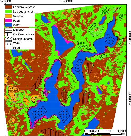
2. Study Area

The Mecklenburg Lake District in northeastern Germany bares the highest density of lakes in Germany. The lake test site, Fürstenseer (FS), is located near Neustrelitz in Mecklenburg-Vorpommern, Germany (Figure 1). The lithospheric basis of its catchment is sandur from the last ice age [29]. The lake is fed by groundwater and has no active inlet or outlet. Like many lakes in the region, it is characterized by seasonal and inter-annual lake level changes [29,30]. Lake FS is well researched [9,30,31,32,33,34] and representative for many lakes in the region. The lake level and ice coverage are measured daily in the southwestern part of the lake by the State Agency for Agriculture and Environment of the Mecklenburg Lake District. The average depth of the lake is 8.0 m; the maximum depth is 24.5 m, while the lake is located 63.5 m above sea level (a.s.l.) [9].

The shoreline of the lake is heterogeneous with respect to land cover and shoreline topography, and is little influenced by human activity, except for small bathing sites in the southwest and southeast areas of the lake. The shoreline topography varies with very shallow areas in the southern part and steeper shorelines in the northeastern part of the lake [9] (cf. Figure 2). The shallow shorelines in the southwest of the lake are densely covered with reeds, as is visible in Figure 3, whereas the southeastern is part only sparsely covered. This difference may be caused by lake level changes in the last decade and the use of the southeastern shoreline as a bathing site. The lake level changes in the last decade ranged around 1 m (cf. Figure 4): in October 2006 the lake level fell to a local minimum of 63.4 m a.s.l. In 2011 there was a significant increase, causing the level to range around 63.8 m (cf. [29,33]). Shallow shoreline areas and a sandbank fell dry during the local minimum in 2006/2007 [9]. The southeastern shoreline was at this time a sandy beach without reed vegetation. Generally, the reed belts at the shoreline move with the decreasing and rising lake level, as long as the changes are not too abrupt [1,35].

3. Available Data

3.1. Dual-Polarimetric (HH, VV) TerraSAR-X Time Series

For this study, we acquired 19 dual-polarimetric (HH, VV) TSX Stripmap images between August 2014 and May 2015. Four images were acquired in ascending orbit (asc), 15 in descending orbit (desc) (see Figure 1 for coverage). The observation space of polarimetry collapses to a singularity for nadir incidence. In contrast, it widens as the incidence angle increases. Therefore, large incidence angles are preferable in polarimetry, as this maximizes the sensitivity of this observation space [36]. Therefore, one of the highest incidence angles in the operational mode of TSX was used with 40° incidence.

Table 1. Overview of the available TerraSAR-X (TSX) data. The mean incidence angle is extracted from the TSX metadata file, the noise equivalent sigma zero (NESZ) and signal-to-noise ratio (SNR) of the images are estimated empirically (as explained above). Additional information about Lake Fürstenseer, provided by the State Agency for Agriculture and Environment of Mecklenburg Lake District, are listed as well.

Date	Mean Incidence Angle (°)	Orbit	NESZ HH (dB)	NESZ VV (dB)	SNR HH (dB)	SNR VV (dB)	Comments
4 August 2014	38.5	Desc	−20.19	−20.32	10.81	10.80
7 August 2014	42	Asc	−19.61	−19.74	8.92	9.06
15 August 2014	38.5	Desc	−20.66	−20.93	9.95	9.82
6 September 2014	38.5	Desc	−20.47	−20.69	9.54	9.35
28 September 2014	38.5	Desc	−20.55	−20.91	9.17	8.96
9 October 2014	38.5	Desc	−20.41	−20.40	10.58	10.21
20 October 2014	38.5	Desc	−19.56	−18.79	8.76	7.60
31 October 2014	38.5	Desc	−21.03	−21.38	9.77	9.61
11 November 2014	38.5	Desc	−21.01	−21.34	9.80	9.52
14 November 2014	42	Asc	−19.40	−18.36	7.91	6.88
22 November 2014	38.5	Desc	−21.12	−21.35	9.47	9.23
25 November 2014	42	Asc	−20.21	−20.10	8.45	8.34
18 February 2015	38.5	Desc	−19.87	−19.86	9.03	8.54	Lake borders covered by ice
1 March 2015	38.5	Desc	−20.94	−20.80	9.43	8.92
12 March 2015	38.5	Desc	−21.01	−21.36	9.61	9.53
23 March 2015	38.5	Desc	−20.87	−21.23	9.91	9.86
26 March 2015	42	Asc	−19.99	−19.81	8.70	8.45
3 April 2015	38.5	Desc	−20.54	−20.55	9.78	9.42
6 May 2015	38.5	Desc	−20.43	−20.85	10.48	10.53

gives an overview on the data of the TSX time series.

The TSX images were delivered in Single Look Slant Range Complex (SSC) format. The pre-processing of the images was implemented in the Interactive Data Language (IDL). First, the images were imported and radiometrically calibrated. Then, intensity-based and polarimetric parameters were calculated according to Equations (3)–(17) (cf. Section 4.1). For spatial averaging during the calculation of the 2 × 2 coherency matrix T_2×2 in Equation (1), we used a sliding window with a 43 × 7 pixels window size, so that the equivalent number of looks (ENL) exceeds the recommended value of 80 [37]. The geocoding of the images was performed using the georeferencing points included in the delivered TSX data. The point-based geocoding was chosen as an appropriate processing standard because the study area is flat with very little topography. The ground range resolution of the asc images is 1.7 m and for the desc images it is 1.9 m. The average azimuth resolution of both orbits is 6.6 m. The grid size of the geocoded images is assigned to 3 m × 3 m. Finally, the images were mapped to WGS 1984, UTM 33 N for comparison with orthophotos.

Before classification of the scenes, we estimated the noise empirically on two regions of interest (roi). Therefore, we selected a homogeneous water area (~3300 pixels) and a homogeneous coniferous forest (~3900 pixels). The empirically-based noise equivalent sigma zero (NESZ) is estimated by the mean intensity acquired over the calm lake bodies (in decibel, dB) and is based on the fact that smooth water should have no backscatter signal at the X-band. The NESZ in our images is always smaller than −18.3 dB, which corresponds to the specified NESZ of dual-polarimetric TSX Stripmap images with −19 dB [38]. The HH and VV backscattering of the reed areas remains largely above −12.5 dB, and only in winter with ice cover it decreases to −14 dB. The empirically estimated signal-to-noise ratio (SNR), as the mean of the intensity of the forest area divided by the mean of the intensity of the water area, ranges between 7 and 11 dB (Table 1). Thus, the signal is ~10 times higher than the noise and therefore no significant noise bias is expected.

3.2. Validation and Training Data

Based on the different scattering mechanisms of natural vegetation (cf. Section 1), we selected five main classes for the study area: open water, deciduous and coniferous forest, meadow, and reed. Bare soil and shrubs are only present in small-scale areas within the study region. Towns and cities are not selected as their own class as the focus is on natural lake regions. The validation areas of reed, water and meadow were digitized based on a digital orthophoto (40 cm resolution, DOP40) from the summer of 2013. For the digitization of the coniferous and deciduous forest validation areas, an additional digital orthophoto (20 cm resolution, DOP20) from winter 2011 was used. The orthophotos were provided by the State Agency for Internal Administration of Mecklenburg-Vorpommern. The validation areas and the training points are illustrated in Figure 2. The sizes of the validation areas are approximately: 29 ha for open water, 30 ha for deciduous forest, 35 ha for coniferous forest, 11 ha for meadow, and 18 ha for reed. Within those validation areas, we selected 30 points for training of the random forest classifier.

The reed area in the southwestern part of the lake was documented during field campaigns with photos in June 2014, November 2015, and January 2016 (Figure 3). Since 2015, the northeastern part of the lake was monitored with a time lapse video.

4. Methods

4.1. Introduction to the Theory of Dual Polarimetry and Its Scattering Parameters

Dual polarimetry is a polarimetric subspace of full or quad polarimetry (HH, HV, VH, VV) [11,39].

In this study, we analyzed 16 dual-polarimetric (HH, VV) parameters with respect to their potential for monitoring reeds (cf.

Table 2. Overview of the 16 parameters derived from the dual-polarimetric TSX data.

Parameter	Abbreviation	Unit	Range
Intensity of HH channel	δHH	Decibel (dB)	−25‒5
Intensity of VV channel	δVV	dB	−25‒5
Intensity of HH plus Intensity of VV	δHH+VV	dB	−25‒5
Intensity of HH minus Intensity of VV	δHH-VV	dB	−25‒5
Intensity ratio HH/VV	δHH/VV	dB	−25‒5
Coherence HHVV amplitude	$\left|{\gamma }_{HHVV}\right|$	-	0‒1
Coherence HHVV phase	$\angle {\gamma }_{HHVV}$	radian	−π‒π
Intensity XX (pseudo)	${\mathsf{\delta }}_{XX, pseudo}$	dB	−25‒5
Dual-polarimetric mean alpha angle	${\overline{\propto }}_{dual}$	Degree (°)	−180‒180
Dual-polarimetric dominant alpha angle	${\propto }_{dual}$	Degree (°)	−180‒180
Entropy	$H_{dual}$	-	0‒1
Anisotropy	$A_{dual}$	-	0‒1
H-A-combination 1	$m1$	-	0‒1
H-A-combination 2	$m2$	-	0‒1
H-A-combination 3	$m3$	-	0‒1
H-A-combination 4	$m4$	-	0‒1

). We calculated different indices based on the HH and VV intensities as well as the dual-polarimetric coherency matrix (cf. Equation (1)), including dominant and mean alpha scattering angles, entropy and anisotropy (normalized eigenvalue difference), plus entropy-anisotropy-combinations (H-A-combinations) .

A state-of-the-art method for quad-polarimetric decomposition is the mathematically-based entropy/anisotropy/alpha (H/A/α) decomposition by Cloude and Pottier [40], which uses eigenvalue/eigenvector analysis of the coherency T matrix for scattering mechanism analysis. The (H/A/α) quad-polarimetric decomposition was later transferred by Cloude to an entropy/alpha (H2α) decomposition for dual-polarimetric data [41]. For this study we use the modified version of the (H2α) decomposition for the 2 × 2 coherency matrix $T_{2x2}$, as defined in Voormansik et al. [20]:

$$T_{2x2}=\frac{1}{2} \langle \left[\begin{array}{cc}(S_{HH}+S_{VV}){(S_{HH}+S_{VV})}^{*}& (S_{HH}+S_{VV}){(S_{HH}-S_{VV})}^{*}\\ (S_{HH}-S_{VV}){(S_{HH}+S_{VV})}^{*}& (S_{HH}-S_{VV}){(S_{HH}-S_{VV})}^{*}\end{array}\right]\rangle$$

(1)

Based on the eigenvalues ${\lambda }_1$ and ${\lambda }_2$and the corresponding eigenvector ${\upsilon }_1$ of the $T_{2x2}$ coherency matrix, the dual-polarimetric entropy ($H_{dual}$), the dual-polarimetric anisotropy ($A_{dual}$), the dominant scattering alpha angle (${\propto }_{dual}$), and the mean scattering alpha angle (${\overline{\propto }}_{dual}$) are calculated (Equations (2)–(6)) [41]. $P_1$ and $P_2$ are the probabilities, ${\chi }_1$ is the first coordinate of the first eigenvector, and $\left|{\upsilon }_1\right|$ is the length of the first eigenvector [41]:

$$P_1=\frac{{\lambda }_1}{{\lambda }_1+{\lambda }_2}, P_2=\frac{{\lambda }_2}{{\lambda }_1+{\lambda }_2}$$

(2)

$$H_{dual}= -(P_1(\frac{{\log }_{10}{P}_1}{{\text{log}}_{10}2})+P_2(\frac{{\log }_{10}{P}_2}{{\text{log}}_{10}2}))$$

(3)

$$A_{dual}=\frac{{\mathsf{\lambda }}_1-{\mathsf{\lambda }}_2}{{\mathsf{\lambda }}_1+{\mathsf{\lambda }}_2}$$

(4)

$${\propto }_{dual}= ={\cos }^{-1}\frac{\left|{\chi }_1\right|}{\left|{\upsilon }_1\right|}$$

(5)

$${\overline{\propto }}_{dual}=P_1{\propto }_{dual}+P_2(\frac{\pi }{2}-{\propto }_{dual})$$

(6)

Based on the intensities of the HH and VV channels, we calculated different indices (in dB) (Equation (7)–(9)). In Equations (10) and (11), the intensities of the HH and the VV channels (in dB) are expressed as well.

$${\mathsf{\delta }}_{HH/VV}=10{\log }_{10}\frac{\langle {\left|S_{HH}\right|}^2\rangle }{\langle {\left|S_{VV}\right|}^2\rangle }$$

(7)

$${\mathsf{\delta }}_{HH-VV}=10{\log }_{10}(\langle {\left|S_{HH}\right|}^2\rangle -\langle {\left|S_{VV}\right|}^2\rangle )$$

(8)

$${\mathsf{\delta }}_{HH+VV}=10{\log }_{10}(\langle {\left|S_{HH}\right|}^2\rangle +\langle {\left|S_{VV}\right|}^2\rangle )$$

(9)

$${\delta }_{HH}=10{\log }_{10}(\langle {\left|S_{HH}\right|}^2\rangle )$$

(10)

$${\delta }_{VV}=10{\log }_{10}(\langle {\left|S_{VV}\right|}^2\rangle )$$

(11)

The dual-polarimetric coherence between HH and VV channels is given in Equation (12) as a complex number. Therefore, ${\gamma }_{HHVV}$ provides the coherence amplitude $\left|{\gamma }_{HHVV}\right|$ and the coherence phase $\angle {\gamma }_{HHVV}$ for analysis [20].

$${\gamma }_{HHVV}=\frac{\langle S_{VV}{S_{HH}}^{*}\rangle }{\sqrt{\langle {\left|S_{HH}\right|}^2\rangle \langle {\left|S_{VV}\right|}^2\rangle }}$$

(12)

Assuming azimuthal symmetry for volume scattering and reflection symmetry for ground scattering also allows the synthesization of the intensity of the cross-polarization ${\mathsf{\delta }}_{XX, pseudo}$ (in dB) from coherent co-polarization data using the coherence ${\gamma }_{HHVV}$ as follows [22,42,43,44]:

$${\mathsf{\delta }}_{XX, pseudo}=10{\log }_{10}(\frac{1}{4}·(1-\left|{\gamma }_{HHVV}\right|)·\langle {\left|S_{HH}-S_{VV}\right|}^2\rangle )$$

(13)

Hence, the information quality of the synthesized cross-polarization intensity can only be as good as the symmetry assumptions on the scatterers is valid for the respective resolution cell.

Finally, we calculated dual-polarimetric H-A-combinations (Equations (14)–(17)) derived equivalently such as for a quad-polarimetric (H/A/α) decomposition [11]. For quad-polarimetric images $(1-H)(1-A)$ corresponds to the presence of a single dominant scattering mechanism, $AH$ to the presence of two scattering mechanisms with the same probability, $A(1-H)$ to the presence of two unequally probable scattering mechanisms, and $H(1-A)$ indicates random scattering [11]. For dual-polarimetric H-A-combinations, the interpretation has not been researched yet, as the dual-polarimetric anisotropy is not a measure of secondary scattering mechanisms. Therefore, a direct allocation to the quantity of scattering mechanisms involved in the scattering process is not possible in the moment and the combinations are named as:

$$m1=(1-H_{dual}) (1-A_{dual})$$

(14)

$$m2=H_{dual}{A}_{dual}$$

(15)

$$m3=A_{dual}(1-H_{dual})$$

(16)

$$m4=H_{dual}(1-A_{dual})$$

(17)

4.2. Random Forest Classification

The classification of the polarimetric SAR images is performed using the random forest (RF) algorithm [45] implemented in R [46]. It is a state-of-the-art method for the classification of remote sensing images and has been successfully used for the classification of PolSAR images of wetland regions [12,17,18] and crop type [47,48] mapping. RF is an ensemble learning method and is based on the construction of a large number of decision trees based on training data. The RF classifier can be trained on very high dimensional datasets, without significant overfitting, and the classifier is also relatively robust to outliers and noise [45] which is important for the spatially variable SAR data. In this study, we selected 30 points for each class as training data for the RF classifier. The position of the training points is illustrated in Figure 2. The minimum distance between the points is 5 m to avoid sampling within the same pixel. The classes are open water, deciduous forest and coniferous forest, meadow, and reed (cf. Section 3.2). About two-thirds of the training points are randomly selected and used for the construction of each decision tree. The remaining training points are used, respectively, as input for each decision tree to generate a test classification for error estimation (out-of-bag error) [45,49]. After a large number of trees is generated (in this study: 500), their different classification results for input are compared and the most popular class (“majority vote”) is assigned as the classification output [45].

Another advantage of the RF classifier is the possibility to assess the importance of each classification parameter (variable) in the classification [45,46]. We chose the “mean decrease in accuracy” as the importance measure as it takes into account the impact of each predictor variable individually as well as its interaction with the other input variables [49]. The importance of a variable is handed out as the mean decrease in the accuracy of the classification. It is calculated during the out-of-bag error calculation phase of the RF classification and represents the difference between the prediction accuracy before and after permuting the variable of interest. The mean decrease in accuracy is given for each class separately (=local importance of a variable) [46]. These importance measures have also been used for feature selection in the classification of polarimetric images [12,49,50]. In this study, we use the information about the importance of a variable to evaluate and score different polarimetric parameters for the classification of reed. As the importance values of the variables may vary with each run, we run the RF classifier 10 times and average the importance values for the analysis.

To test the accuracy of the different polarimetric SAR parameters, the RF classifier was applied on different combinations of polarimetric parameters:

• Single parameter images: every parameter at every date
• Parameter stacks: stack of all kinds of parameters of a date
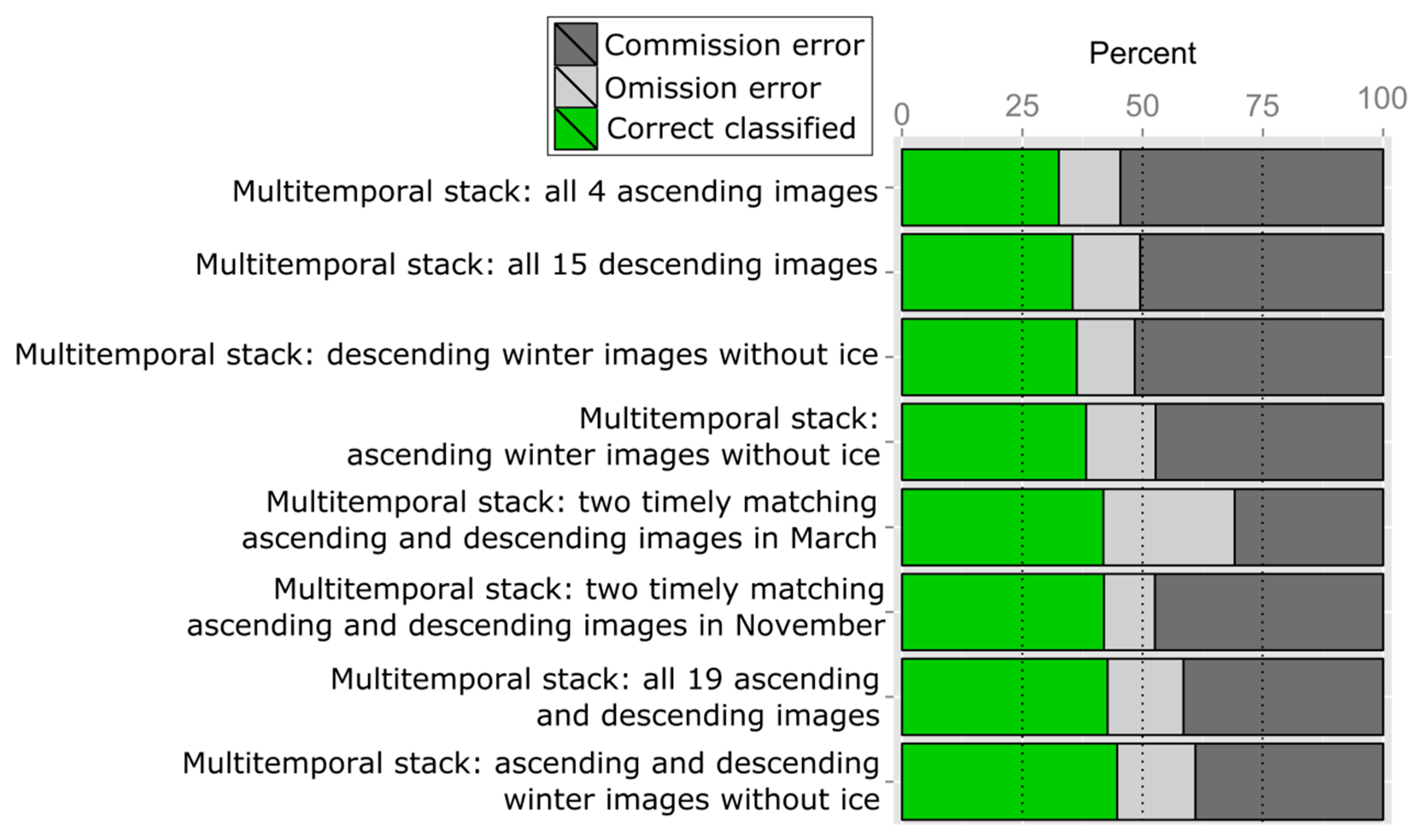
• Multi-temporal parameter stacks: stack of all kinds of parameters of multiple dates (with different look directions)

  -

  all 19 asc and desc images;

  -

  all 15 desc images;

  -

  all four asc images;

  -

  asc and desc winter images without ice (31 October 2014, 11 November 2014, 14 November 2014, 22 November 2014, 25 November 2014, 12 March 2015, 23 March 2015, 26 March 2015);

  -

  asc winter images without ice (14 November 2014, 25 November 2014, 26 March 2015);

  -

  desc winter images without ice (31 October 2014, 11 November 2014, 22 November 2014, 12 March 2015, 23 March 2015);

  -

  two timely matching asc and desc images in November (14 November 2014 and 22 November 2014);

  -

  two timely matching asc and desc images in March (26 March 2015 and 23 March 2015).

Before the classification of the multi-temporal parameter stacks, the stacks were masked to retrieve the overlaying area of the asc and desc scenes. The polygon is irregular, but the not available (NA) values in the stacked images are not considered within the RF classification.

4.3. Evaluation of the Classification

For validation of the reed area, the classification results were cut to match with the lake area and its close surroundings. Therefore, we used the water-land border of the lake plus a 50 m buffer around the lake area. Within this lake area we calculated the intersection of the validation reed area and our classification results as the correct classified reed area. Additionally, we calculated the commission area (false positive classified as reed) and the omission area (missed reed areas, false negative). For better comparison of the time series data, we then calculated the correct classified proportion, the commission error and the omission error in percent (correct classified + commission error + omission error = 100%).

5. Results and Discussions

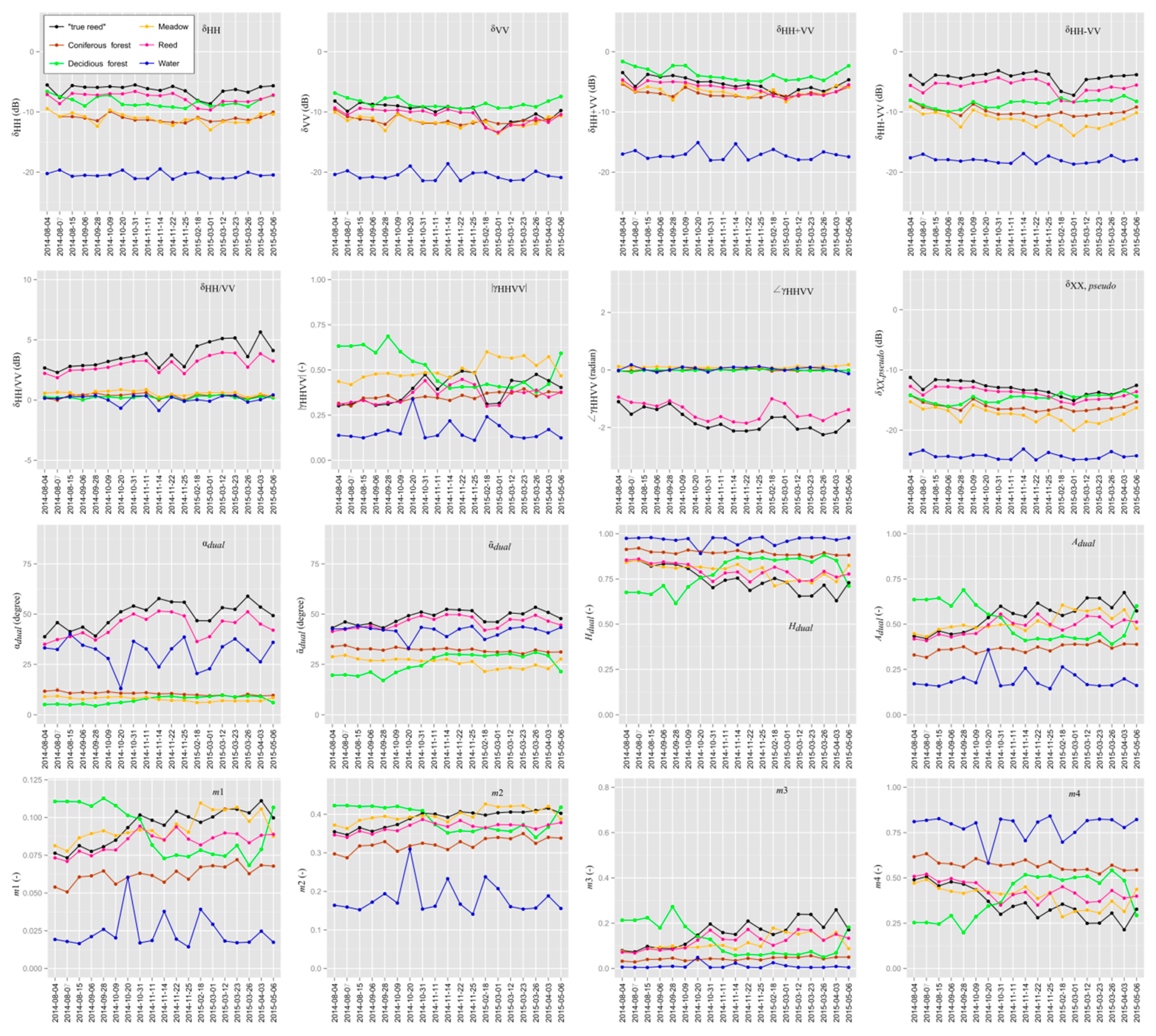
5.1. Time Series Analysis of the Validation Areas

Figure 5 shows the mean values of each parameter for each validation area (deciduous and coniferous forest, water, meadow, and reed). Additional to the reed validation area, the mean of the “true reed” area is illustrated in dark pink. The “true reed” area is the correct classified reed area that denotes the intersection of the reed area of the RF classification of the parameter stacks (cf. Section 5.3) and the validation reed area. The change of the study area in summer and winter is illustrated in Figure 6 with two RGB images (δ_HH-VV, $\left|{\mathsf{\gamma }}_{\text{HHVV}}\right|$, and ${\overline{\propto }}_{dual}$).

First, we will analyze the changes of reed during the year on the basis of Figure 5. Generally, the “true reed” mean has a similar curve progression as the reed area, but it is shifted and better separated from the other classes. Thus, for the analysis of the phenology, we will concentrate on the “true mean” values because of the less disturbed reed signal.

The phenology of reed is characterized by strong growth in April (mainly stem) and May (stem and leaves). By the end of June the maximum leave area is reached. In August the reed blooms and only the rhizome continues to grow [2,51]. Between October [51] and November/December [2], depending on the literature, the leaves of the reed start to wither and fall off. On 11 November 2015 the leaves were withered, but most were still attached to the stems (Figure 3). Unfortunately, no photos were taken at the end of 2014, so the actual phenological state of the reed in November 2014 is unknown. The withered stems of the reed keep standing [1,2] unless they are cut off by moving ice. The cut off of reed is very unlikely in the study area, according to an expert (Peter Stüve) for Lake Fürstenseer See. The time lapse video vaguely shows the development of the first leaves on the reed and the very clear development of the leaves of the deciduous trees between 9 April 2015 and 6 May 2015.

Thus, in summer we expect mainly volume scattering at the X-band coming from the complex structure of the leaves and stems in the reed vegetation [19]. In winter and early spring (until early March), we expect predominantly double-bounce scattering from the remaining stems and the lake surface underneath. In May, the development of the reed leaves increases the volume scattering component again. It needs to be considered that our TSX time series does not cover the entire year: there have been no acquisitions in December, January, June, and July.

Generally, the majority of the 16 parameters show a similar trend of high (respectively low) values in August/September, then a decrease (increase) in October, low (high) values in November and March and finally another increase (decrease) in April/May. Outliers are the dates 18 February 2015 and 1 March 2015. On 18 February 2015, the borders of the lake were covered by ice. However, due to the similarity of the polarimetric parameters (e.g., coherences, alpha angles and intensities) on 18 February 2015 and 1 March 2015, we assume that there is still ice coverage on 1 March 2015 on some lake borders. In the following analysis, the acquisitions with ice on 18 February 2015 and 1 March 2015 are excluded due to a very different scattering behavior. The remaining images are then all ice- and snow-free. The differences between summer (August, September) and winter/early spring (November/beginning of March) are listed in

Table 3. Difference of the mean values and standard deviation of the “true reed” area in summer (August, September) and winter/early spring (November/March).

Parameter	Summer	Winter, Early Spring
${\mathsf{\delta }}_{HH/VV}$ (only desc images)	2.81 ± 0.09 dB	4.47 ± 0.67 dB
${\mathsf{\delta }}_{XX,pseudo}$	−11.92 ± 0.69 dB	−13.60 ± 0.39 dB
$\left|{\gamma }_{HHVV}\right|$	0.31 ± 0.01	0.45 ± 0.03
$\angle {\gamma }_{HHVV}$	−1.29 ± 0.15 rad	−2.07 ± 0.10 rad
${\overline{\propto }}_{dual}$	44.4° ± 1.2°	51.4° ± 1.3°
${\propto }_{dual}$	41.7° ± 30°	55.2° ± 2.5°
$H_{dual}$	0.84 ± 0.01	0.71 ± 0.04
$A_{dual}$	0.44 ± 0.01	0.60 ± 0.04
$m1$	0.08 ± 0.00	0.10 ± 0.00
$m2$	0.36 ± 0.01	0.40 ± 0.01
$m3$	0.09 ± 0.01	0.19 ± 0.03
$m4$	0.48 ± 0.02	0.30 ± 0.04

. No significant seasonal trend is present in the temporal evolution of the parameters ${\mathsf{\delta }}_{HH}$, ${\mathsf{\delta }}_{VV}$, ${\mathsf{\delta }}_{HH-VV}$, and ${\mathsf{\delta }}_{HH+VV}$.

The phenological changes can be clearly seen in parameters that are sensitive to the double-bounce-scattering mechanism, such as ${\mathsf{\delta }}_{HH/VV}$, $\angle {\gamma }_{HHVV}$, ${\overline{\propto }}_{dual},$ and ${\propto }_{dual}$. However, δ_HH-VV, which is also sensitive to double-bounce scattering, does not correlate to the phenological changes, but has high values (mean: −4 dB) during the entire monitoring period. Surprising are also the significant differences between asc and desc images of the parameter ${\mathsf{\delta }}_{HH/VV}$: for desc images, the${\mathsf{\delta }}_{HH/VV}$ shows an increase in winter, correlated to more prominent double-bounce scattering. The parameter $\angle {\gamma }_{HHVV}$ of reed is around −1.3 rad in summer and decreases in winter to values mostly smaller than −2 rad. This would be in line with quad-polarimetric studies that show that a phase shift of about |π| rad indicates double-bounce [49]. The ${\overline{\propto }}_{dual}$ of reed ranges between 40° (summer) and 50° (winter, without ice); the ${\propto }_{dual}$ reaches 60° in winter/early spring. For quad-polarimetric SAR, pure double-bounce as the dominant scatter mechanism is indicated by alpha angles close to 90° [18]. In this study, we also interpret the increase of the dual-polarimetric alpha angle values in winter as a consequence of an increasing proportion of double-bounce scattering. The parameter $\left|{\gamma }_{HHVV}\right|$ refers to the correlation of HH and VV intensities: here, our study shows that in summer the $\left|{\gamma }_{HHVV}\right|$ of reed belts (“true reed”) is lower (~1.5) than in winter without reed leaves. The cross-polarimetric channel predominantly shows vegetation scattering and is sensitive to the amount of biomass [20,52]. The ${\mathsf{\delta }}_{XX,pseudo}$ of reed is therefore lower in winter than in summer, because of the leaf-off period within the reed belts.

The $H_{dual}$ and $A_{dual}$ and, consequently, also $m1,$ $m2,$ $m3,$ and $m4$ values of reed change throughout the year. The $A_{dual}$ and the combination parameters ($m1,$ $m2,$ $m3,$ and $m4$) are new and the interpretation is therefore still speculative: following the interpretation of quad-polarimetric entropy $H$and anisotropy $A,$ a high $H$ and low $A$ correspond to random scattering, whereas a high $H$ together with a high $A$ correspond to the presence of two equal scattering mechanisms [11]. In summer $H_{dual}$ is significantly larger than $A_{dual}$, probably corresponding to volume scattering. In winter both $H_{dual}$ and $A_{dual}$ are characterized by larger fluctuations, which make the interpretation difficult. However, generally, $A_{dual}$ has higher values and is closer to $H_{dual}$ which indicates a change of the scattering mechanism in winter. Our study shows the importance of the mutual use of $H_{dual}$ and $A_{dual}$, as in a previous PolSAR study of rice with high dual-polarimetric entropy values (~0.9) in spring and which, in the end of the vegetative phase, could not be differentiated. It was suggested that high dual-polarimetric entropy values (~0.9) in spring were a result of the mixed scattering of the surface and double-bounce, and high dual-polarimetric entropy values in the end of the vegetative phase were a result of random scattering generated by the plants’ volume [24], but for better interpretation the calculation of $A_{dual}$ is useful. For quad-polarimetric images, $m4$ indicates random scattering [11], and also for reed, $m4$ decreases in winter, whereas the dual-polarimetric H-A-combinations $m1,$ $m2$ and $m3$ increase. This could be interpreted as an increase of the presence of single, dominant scattering processes and the two-scattering mechanism because of the double-bounce of reed in winter, but further studies are necessary to validate these purely empirical observations.

As shown above, the phenology of reed changes the polarimetric parameter in winter and summer, but deciduous forest and meadow also show seasonal changes. Additionally, changing environmental conditions such as partial ice coverage of the lake on 18 February 2015 and probably 1 March 2015 influence the separability of the five classes.

The best separation of reed areas from the other classes by the mean values of the observed parameters is achieved in winter by the double-bounce–sensitive parameters ${\mathsf{\delta }}_{HH-VV}$, ${\mathsf{\delta }}_{HH/VV}$, $\angle {\gamma }_{HHVV}$, ${\overline{\propto }}_{dual}$ and ${\propto }_{dual}$. Especially ${\mathsf{\delta }}_{HH-VV}$ and ${\mathsf{\delta }}_{HH/VV}$ have proven useful in the classification of flooded vegetation in [25,53]. The mean values of ${\propto }_{dual}$ are more extreme than the mean values of ${\overline{\propto }}_{dual}$ and the seasonal variation of the parameter ${\propto }_{dual}$ is more pronounced. Hence, ${\propto }_{dual}$ appears more suitable for the separation of reed according to the investigations in Figure 5. Reed has predominantly the highest mean ${\mathsf{\delta }}_{HH}$ values and they are higher than ${\mathsf{\delta }}_{VV}$ during the entire monitoring period (cf. [25]). However, ${\mathsf{\delta }}_{HH}$ has a high probability of confusion with deciduous forest because, especially in spring, the mean values of ${\mathsf{\delta }}_{HH}$differ only by 2 dB to the ones of reed. The parameter ${\mathsf{\delta }}_{XX,pseudo}$, is an indicator of vegetation scattering [20,52], and also reacts to reed as well as forest. Thus, ${\mathsf{\delta }}_{HH}$ and ${\mathsf{\delta }}_{XX,pseudo}$ are very suitable for the distinction of reed and water (no volume scattering on the lake surface), but not for the distinction of reed and deciduous forest. Another problem is the dependence on the look direction of the co-polarized intensities (HH, VV): in Figure 6 the dependency of the look direction results in higher values near the shorelines in the range direction in channel δ_HH-VV. $H_{dual}$ and $A_{dual}$, and consequently also the scattering mechanism from the dual-polarimetric H-A-combinations, show a high similarity of reed and meadow, probably because of a similar phenology. During leaf fall and growth, confusion with scattering from deciduous forest is also possible. As such, ${\mathsf{\delta }}_{VV}$,${\mathsf{\delta }}_{HH+VV}$, and $\left|{\gamma }_{HHVV}\right|$ are the parameters that are least distinct in their mean values. They have a high likelihood of confusion of reed with other various classes. Thus, ${\mathsf{\delta }}_{HH+VV}\text{ indicates}$ direct surface or odd-bounce scattering [25] and the mean value for reed is, in winter, nearly identical with the values for scattering from meadows and coniferous forest. In summer, the mean value of reed lies between the mean value of deciduous forest and the values of meadow and coniferous forest, but the probability for confusion is still critical. The parameter $\left|{\gamma }_{HHVV}\right|$ of reed is, in summer, nearly identical with that of coniferous forest; the rest of the year, $\left|{\gamma }_{HHVV}\right|$ of reed is also similar to those of meadow and deciduous forest.

5.2. RF Classification: Single Parameter Layer of Every Date

Here, we start with the actual classification, after the analysis of the observed polarimetric parameters by the mean values of the classes. This is important, as the mean values do not represent the spatial variability of these parameters. Therefore, we test the potential of every parameter for reed mapping by classifying every single parameter image using RF classification. The classifications of every parameter at every date result in $6·19=304$ classifications.

For the evaluation of the classification results, we calculated the correct classified proportion of reed (correct positive), the commission error (false positive) and omission error (false negative) in percent based on the validation reed area. For the temporal evaluation, we stacked the correct classified proportions of each date (Figure 7a), the commission errors of each date (Figure 7b), and the omission errors of each date (Figure 7b). The higher the stacks in Figure 7a, the better the reed classifications of the different parameters are and the more valuable the date is for the classification of reed.

In line with the results of Section 5.1, there is a significant difference in Figure 7a between the winter and early spring dates (between 20 October 2014 and 3 April 2015) and the summer and late spring dates (4 August 2014 and 9 October 2014 and on 6 May 2015). The winter and early spring dates have better classification results and the best results are achieved on 22 November 2014. Outliers are, again, 18 February 2014 and 1 March 2014, the dates with (assumed) partial ice cover. A difference between asc images (grey date labels) and desc images (black date labels) is not apparent.

In Figure 7a, ${\mathsf{\delta }}_{HH/VV}$, ${\mathsf{\delta }}_{HH-VV}$, ${\overline{\propto }}_{dual}$, and $\angle {\gamma }_{HHVV}$show the best classification results with >25% correctly classified reed areas. The parameter ${\mathsf{\delta }}_{HH/VV}$achieves the best results, with 32% correctly classified reed area. This result fits with the good separation of the reed mean values from all other classes (Figure 5). The mean value of ${\propto }_{dual}$ was also clearly distinguishable from other classes (Figure 5), but the RF classification results mainly in low accuracies due to the typically high spatial variability of the parameter [20], also misclassified as noise in the water area. The ${\overline{\propto }}_{dual}$ is not as pronounced as ${\propto }_{dual}$, but it is also less spatially varying and is therefore more suitable for classification. The performances of some parameters vary significantly during the year: ${\mathsf{\delta }}_{HH-VV}$ has higher accuracies in summer, ${\mathsf{\delta }}_{HH/VV}$ in winter. The parameters $H_{dual}$, $\angle {\gamma }_{HHVV}$, $A_{dual}$, $m3,$and $m4$perform better in winter, whereas ${\mathsf{\delta }}_{HH}$ and ${\mathsf{\delta }}_{XX,pseudo}$ have a better performance in summer. The different accuracies throughout the year are caused by phenological changes of the reed plants, but also other vegetation classes, and therefore cause greater differences between the mean values of the different classes (Figure 5).

The graphs of omission and commission error, as well as a visual check of the 304 maps (cf. Supplements, Heading 1), show that different parameters have different error behavior: the intensity parameters have higher commission errors, caused by bright backscatter values around the lake in range directions. Parameters ${\overline{\propto }}_{dual}$ and ${\propto }_{dual}$ and $\angle {\gamma }_{HHVV}$ have high commission errors, mainly caused by misclassified noise in the open water area of the lakes. Additionally, the high spatial variability of ${\propto }_{dual}$, and also of $\angle {\gamma }_{HHVV}$, is another source of error. As expected from the comparison of the mean values in Section 5.1,$H_{dual}$ and $A_{dual}$, and consequently also $m1$, $m2$, $m3$ and $m4$, have a high omission error, caused by the confusion of reed with meadows. The same characteristics occur for $\left|{\gamma }_{HHVV}\right|$.

The classification of the single parameter images emphasizes the significant influence of the spatial homogeneity of the parameters on the classification, because a good separation of the mean values from the reed belts and from the main other classes does not automatically come with good classification results for reed. Hence, the high spatial variability of the observed polarimetric parameters is a significant source of error.

5.3. RF Classification with Parameter Stacks for One Date

After the analysis of the individual parameters, we now analyze the parameter stacks of each date. Figure 8 presents the correct classified proportion of reed in a stacked way, together with the commission and omission errors of each date. The highest correctly classified proportions (35%–36%) of reed acquisitions were obtained on 14 November 2014, 26 March 2015 (asc images) and 22 November 2014 (desc images). The commission error is mostly over 50%; thus, reed areas are frequently overestimated, and reasons for the overestimation are discussed later in this chapter. On 18 February 2014 and 1 March 2014, the dates with partial ice coverage, the correct classified area is over 30%, but the omission error is high.

Figure 9 shows the importance of the parameters (concerning the mean decrease in accuracy) for the classification of the reed. A high mean decrease in accuracy means that the parameter is important for the accurate classification of the class “reed”. However, it needs to be considered that the RF algorithm aims at the most accurate classification of all classes.

The parameter ${\mathsf{\delta }}_{HH-VV}$ is on 15 dates the most important variable, and on the other dates it is one of the five most important variables. Then, ${\mathsf{\delta }}_{XX, pseudo}$ is one of the most important variables in August and September, but it decreases from October onwards in its rank, because other variables (${\mathsf{\delta }}_{HH/VV}$, ${\overline{\propto }}_{dual}$, ${\propto }_{dual}$) become more important. As such, δ_HH+VV is, with one exception, one of the five most important variables in summer. In summer, the dense leaves of the reed cause volume scattering, in addition to double-bounce scattering from the stems. Thus, in summer double-bounce–sensitive parameters are not as valuable in finding reed belts as in winter, and other parameters are chosen by RF classification.

For the 10 ice-free images between 20 October 2014 and 3 April 2015, ${\mathsf{\delta }}_{HH-VV}$ is always one of the five most important variables.. ${\mathsf{\delta }}_{HH}$ and ${\overline{\propto }}_{dual}$ are on eight, ${\mathsf{\delta }}_{HH/VV}$ and ${\gamma }_{HHVV,phase}$ on six, ${\mathsf{\delta }}_{XX, pseudo}$ on four and ${\propto }_{dual}$ on three dates the most valuable variables. Thus, the variable importance for RF classification is determined by the sensitivity to double-bounce scattering and also by the spatial variability of the parameter: the spatially homogeneous parameters ${\mathsf{\delta }}_{HH-VV}$, ${\overline{\propto }}_{dual}$ and ${\mathsf{\delta }}_{HH/VV}$ and the spatially variable parameters ${\gamma }_{HHVV,phase}$, ${\propto }_{dual}$ reach high importance because they react very well to the double-bounce of reed in winter. However, ${\mathsf{\delta }}_{HH}$ and ${\mathsf{\delta }}_{XX, pseudo}$ are spatially homogeneous and partly sensitive to vegetation, and they do not show sensitivity to an increase of double-bounce scattering in the time series.

A high importance of the HV intensity for wetland monitoring was also found in a study by Zhao et al., and in their study, the intensities (HV, HH and VV) were overall more important for accuracy than the quad-polarimetric parameters [12]. We conclude that the higher importance of intensity parameters in Zhao et al. and their high importance in our study is caused by the good distinction of many classes via backscattering and backscatter combinations, as well as their spatial homogeneity. However, polarimetric parameters are important, because they are often specific for one scattering type, and thus improve the classification of specific classes (cf., e.g., Figure 5, $\angle {\gamma }_{HHVV}$ for the distinction of reed).

Figure 10 and Figure 11 show the RF classification of the four dates, with a desc and an asc image for August and November 2014. The high commission errors (~65%) of the classification result in August are caused by an overestimation of in situ reed areas and false-positive classified reed areas at the shorelines in range directions. Water along with mainly deciduous trees are misclassified as reed. The comparison of the asc and desc images (Figure 10) reveals that the overestimations of the reed area in comparison to the validation reed area appear generally in the look direction of the sensor (range direction); thus, the classification result of the asc stack goes too far to the east, whereas the result of the desc image reaches too far to the west. The misclassifications of deciduous forest as reed in Figure 10 and Figure 11 are caused by high backscatter values near the shoreline area, similar to the backscatter of reed (cf. Figure 6), whereas the high commission errors (~60%) of the classification result in November is largely caused by the misclassification of water or deciduous forest located around the reed areas. The overestimation in November is clearly linked to the presence of reed and only locally there are misclassifications related to the sensor look direction. The difference between Figure 10 and Figure 11 is also related to the more prominent double-bounce scattering in winter during the leaf-off season, thus the stronger influence of the double-bounce–sensitive parameters in the classification within this period of the year.

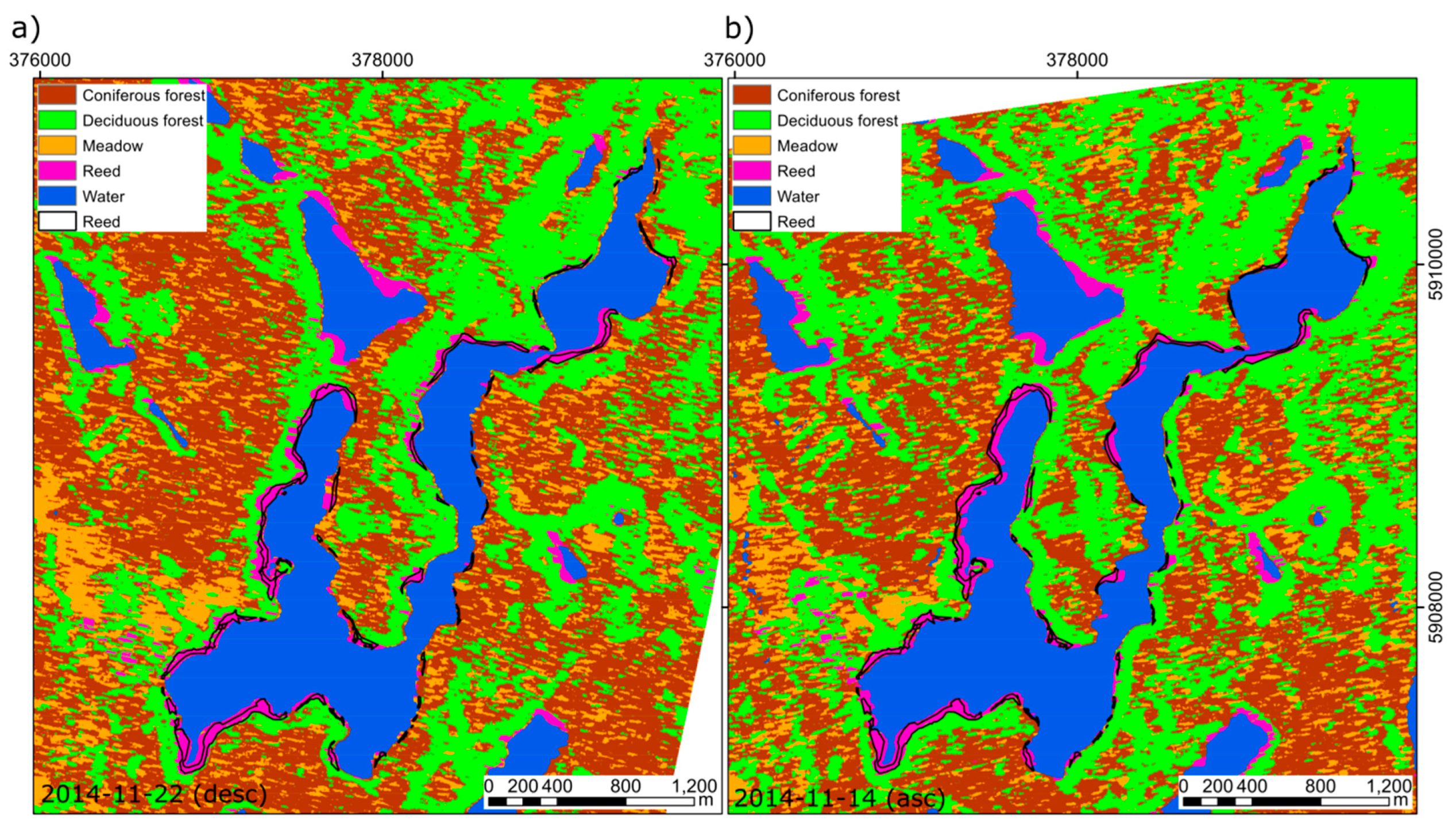
5.4. RF Classification with Multi-Temporal Parameter Stacks

Finally, we tested if the classification accuracy of reed can be improved by using multi-temporal image stacks.

Figure 12 illustrated the classification accuracies of the different multi-temporal stacks. All stacks with a combination of asc and desc images perform better than stacks with only desc or only asc images, because it reduces the impact of the looking direction (cf. Figure 10 and Figure 11). Tests showed that the classification of a multi-temporal stack of asc and desc images has similar (±3% correct classified reed) accuracies as the intersection of the reed areas of the classification results of asc and desc images (cf. Supplements, Heading 2). The highest correct classified proportion (45%) is achieved with the multi-temporal stack of ice-free winter images (asc and desc). The corresponding classification is illustrated in Figure 13. Its confusion matrix is illustrated in

Table 4. Confusion matrix of the random forest classification based on the multi-temporal stack of ice-free winter images (asc and desc). The validation areas used are illustrated in Figure 2. All numbers represent pixels.

		Predicted by Random Forest
		Coniferous Forest	Deciduous Forest	Meadow	Reed	Water
Actual Class	Coniferous forest	36,807	1527	1503	2528	0
	Deciduous forest	1501	30,931	91	2415	0
	Meadow	453	557	10,597	64	0
	Reed	0	181	0	14,440	0
	Water	0	0	0	247	32,706

and the overall accuracy of this classification is 91.90%.

The comparison of Figure 11 and Figure 13 shows that the use of the multi-temporal stack also improves the accuracy of the other classes as compared to single-date classification.

Although, the classification of reed improved through the use of multiple images, the highest correctly classified proportion is only 45%, which is half of the area. For test purposes, we tried a second classification via k-means segmentation. It showed that the k-means classification result of reed is very similar to the one of RF (cf. Supplements, Heading 3) and suggests that the error of over 50% is not caused by the choice of the classification method. Another reason potentially leading to a reduced accuracy of the classification may be found in the small number of training points. This might be too few to fully characterize one class. However, tests with five times more training points (150 instead of 30) only led to an accuracy improvement of 1.65%. We explain the high error with various factors:

The reed belts are small and stretched long, sometimes with tree cover, which can lead to a small feature bias. Tree cover might also lead to errors in the manually digitized reed areas that were used for validation. The classification in Figure 13 clearly shows that small reed areas or reed areas with a very small width (<10 m) are not detected using TSX images, but larger and more extended features are. This is also due to the resolution of TSX of 3 m × 3 m after geocoding. Although missed small reed belts are numerous, they have only a small percentage weight for the commission error. The same is valid for the commission error if misclassified water areas were caused by an expansion of reed areas since 2013. The misclassifications of deciduous forest can be related to the parameter values similar to reed in winter (cf. Figure 5). Quad-polarimetric images might be beneficial here for improving the distinction with their higher information content. However, the misclassifications could also be caused by spatial deviations between the SAR images and the digital orthophoto. The asc and desc SAR images are acquired with different looking directions and with different incidence angles causing different geocoding challenges. As the comparison of asc and desc images emphasizes, the geocoding of the side-looking SAR is challenging, especially at shoreline areas with a large height difference between high trees and the water surface [4]. Thus, we think the main sources of errors are spatial inaccuracies due to geocoding.

6. Conclusions

This study investigates the potential of dual-polarimetric TSX data for mapping and monitoring of reed belts: 13 of the 16 calculated parameters (Table 3) show a significant difference between summer and winter acquisitions caused by the phenology of reed. In summer, the volume scattering of reed belts is high, whereas during the leaf-off season in winter and early spring, double-bounce scattering dominates for the X-band within reed belts. Besides the double-bounce–sensitive parameters (δ_HH/VV, ${\overline{\propto }}_{dual}$, ${\propto }_{dual}$, and $\angle {\gamma }_{HHVV}$), also $\left|{\gamma }_{HHVV}\right|$, $A_{dual }$, $H_{dual }$, $m1, m2, m3$ and $m4$reveal seasonal changes for reed in X-band dual-polarimetric SAR data. Changes of the parameters suggest that phenological stages such as the start of leaves growing around the middle of March and the withering and the falling off of leaves starting around October can be monitored as we’’. However, a more detailed study with a denser time series of TSX images together with a simultaneous in situ documentation of the reed belts and additional measurements, such as the water content of the leaves/stems as well as rain events, is necessary to support this first result. The increase of double-bounce scattering in winter due to the falling-off of leaves enables a better separation of reed and other vegetation (meadow, deciduous and coniferous forest); thus, winter acquisitions (without ice) are preferred for the mapping of reed belts. The five most important parameters for the classification of reed are ${\mathsf{\delta }}_{HH-VV}$, ${\overline{\propto }}_{dual}$, δ_HH/VV, ${\mathsf{\delta }}_{HH}$, and $\angle {\gamma }_{HHVV}$. Except of ${\mathsf{\delta }}_{HH}$; all these parameters are direct indicators of double-bounce scattering. The ${\propto }_{dual}$ would be also an appropriate indicator for double-bounce scatting, but it appeared more spatially variable in the analysis than, e.g., ${\overline{\propto }}_{dual}$. This variability induced classification challenges. Spatial variability seems also to be a problem for $\angle {\gamma }_{HHVV}$ as a monitoring parameter for reed.

The RF classification is fast, easy to implement, and a preselection of classification parameters is not required because the algorithm automatically selects the best parameters for classification. In the comparison of single-date winter images and a multi-temporal winter stack, the multi-temporal winter stack achieved better results for the classification of reed belts. The combination of asc and desc images also improved the classification result, as it reduced the influence of the sensor look direction. However, in this study an accuracy of only ~50% correctly classified reed belts was achieved. The overall classification accuracy of all five classes is 91.90%. The following reasons could be identified. Whereas the shorelines with reed areas (>10 m in width) could be detected correctly, the actual areas with reed coverage were significantly overestimated. The main source of error is probably geocoding with spatial inaccuracies. This error could be reduced with better geocoding and additional pre-processing of the SAR data, e.g., an additional co-registration of the SAR images to the digital orthophotos. However, the optimization of the spatial accuracy went beyond the scope of this study. In this study, the focus was on the process of understanding the scattering mechanisms present in reed belts and their exploitation for classification purposes.

References

1. Bogenrieder, A. Das Schilfrohr (Phragmites australis (Cav.) Trin). Biol. Unserer Zeit 1990, 20, 221–222. [Google Scholar] [CrossRef]
2. Rodewald-Rudescu, L. Die Binnengewässer, Band XXVII, Das Schilfrohr; Stuttgart, Germany, 1974. [Google Scholar]
3. Schmieder, K.; Dienst, M.; Ostendorp, W.; Joehnk, K. Effects of water level variations on the dynamics of the reed belts of Lake Constance. Ecohydrol. Hydrobiol. 2004, 4, 469–480. [Google Scholar]
4. Heine, I.; Francke, T.; Rogass, C.; Medeiros, P.H.A.; Bronstert, A.; Foerster, S. Monitoring Seasonal Changes in the Water Surface Areas of Reservoirs Using TerraSAR-X time series data in semiarid Northeastern Brazil. IEEE J. Sel. Top. Appl. Earth Obs. Remote Sens. 2014, 7, 3190–3199. [Google Scholar] [CrossRef]
5. Bresciani, M.; Stroppiana, D.; Fila, G.; Montagna, M.; Giardino, C. Monitoring reed vegetation in environmentally sensitive areas in Italy. Ital. J. Remote Sens. 2009, 41, 125–137. [Google Scholar] [CrossRef]
6. Schuster, C.; Schmidt, T.; Conrad, C.; Kleinschmit, B.; Förster, M. Grassland habitat mapping by intra-annual time series analysis—Comparison of RapidEye and TerraSAR-X satellite data. Int. J. Appl. Earth Obs. Geoinf. 2015, 34, 25–34. [Google Scholar] [CrossRef]
7. Csaplovics, E.; Nemeth, E. Airborne Optical Imaging in Support of Habitat Ecological Monitoring of the Austrian Reed Belt of Lake Neusiedl. In Proceedings of the GISScience RSGIS4HQ, Vienna, Austria, 24–25 September 2014; pp. 163–167.
8. Lantz, N.J.; Wang, J. Object-based classification of Worldview-2 imagery for mapping invasive common reed, Phragmites australis. Can. J. Remote Sens. 2014, 39, 328–340. [Google Scholar] [CrossRef]
9. Heine, I.; Stüve, P.; Kleinschmit, B.; Itzerott, S. Reconstruction of lake level changes of groundwater-fed lakes in Northeastern Germany using RapidEye time series. Water 2015, 7, 4175–4199. [Google Scholar] [CrossRef]
10. Castree, N.; Demeritt, D.; Liverman, D.; Rhoads, B. A Companion to Environmental Geography; John Wiley & Sons: Chichester, UK, 2009. [Google Scholar]
11. Lee, J.; Pottier, E. Polarimetric Radar Imaging—From Basics to Applications, 1st ed.; CRC Press: New York, NY, USA, 2009. [Google Scholar]
12. Zhao, L.; Yang, J.; Li, P.; Zhang, L. Seasonal inundation monitoring and vegetation pattern mapping of the Erguna floodplain by means of a RADARSAT-2 fully polarimetric time series. Remote Sens. Environ. 2014, 152, 426–440. [Google Scholar] [CrossRef]
13. Smith, L.C. Satellite remote sensing of river inundation area, stage, and discharge: A review. Hydrol. Process. 1997, 11, 1427–1439. [Google Scholar] [CrossRef]
14. White, L.; Brisco, B.; Dabboor, M.; Schmitt, A.; Pratt, A. A collection of SAR methodologies for monitoring wetlands. Remote Sens. 2015, 7, 7615–7645. [Google Scholar] [CrossRef]
15. Betbeder, J.; Rapinel, S.; Corpetti, T.; Pottier, E.; Corgne, S.; Hubert-Moy, L. Multitemporal classification of TerraSAR-X data for wetland vegetation mapping. J. Appl. Remote Sens. 2014, 8, 083648. [Google Scholar] [CrossRef]
16. Schmitt, A.; Brisco, B. Wetland monitoring using the curvelet-based change detection method on polarimetric SAR imagery. Water 2013, 5, 1036–1051. [Google Scholar] [CrossRef]
17. Corcoran, J.; Knight, J.; Gallant, A. Influence of multi-source and multi-temporal remotely sensed and ancillary data on the accuracy of random forest classification of wetlands in Northern Minnesota. Remote Sens. 2013, 5, 3212–3238. [Google Scholar] [CrossRef]
18. Van Beijma, S.; Comber, A.; Lamb, A. Random forest classification of salt marsh vegetation habitats using quad-polarimetric airborne SAR, elevation and optical RS data. Remote Sens. Environ. 2014, 149, 118–129. [Google Scholar] [CrossRef]
19. Yajima, Y.; Sato, R.; Yamada, H.; Boerner, W. Polsar image analysis of wetlands using modified four component scattering decomposition. IEEE Trans. Geosci. Remote Sens. 2008, 46, 1667–1673. [Google Scholar] [CrossRef]
20. Voormansik, K.; Jagdhuber, T.; Olesk, A.; Hajnsek, I.; Papathanassiou, K.P. Towards a detection of grassland cutting practices with dual polarimetric TerraSAR-X data. Int. J. Remote Sens. 2013, 34, 8081–8103. [Google Scholar] [CrossRef]
21. Dusseux, P.; Corpetti, T.; Hubert-Moy, L.; Corgne, S. Combined use of multi-temporal optical and radar satellite images for grassland monitoring. Remote Sens. 2014, 6, 6163–6182. [Google Scholar] [CrossRef]
22. Voormansik, K.; Jagdhuber, T.; Zalite, K.; Noorma, M.; Hajnsek, I. Observations of cutting practices in agricultural grasslands using polarimetric SAR. IEEE J. Sel. Top. Appl. Earth Obs. Remote Sens. 2015, 9, 1382–1396. [Google Scholar] [CrossRef]
23. Lopez-Sanchez, J.M.; Cloude, S.R.; Ballester-Berman, J.D. Rice phenology monitoring by means of SAR polarimetry at X-band. IEEE Trans. Geosci. Remote Sens. 2012, 50, 2695–2709. [Google Scholar] [CrossRef]
24. Lopez-sanchez, J.M.; Ballester-berman, J.D.; Cloude, S.R.; Group, T. Retrieval of Rice Phenology by Means of Sar Polarimetry. In Proceedings of the 5th International Workshop on Science and Applications of SAR Polarimetry and Polarimetric Interferometry, Franscati, Italy, 24–28 January 2011; Volume 2011, pp. 1–8.
25. Lopez-Sanchez, J.M.; Ballester-Berman, J.D.; Hajnsek, I. First results of rice monitoring practices in Spain by means of time series of TerraSAR-X dual-pol images. IEEE J. Sel. Top. Appl. Earth Obs. Remote Sens. 2011, 4, 412–422. [Google Scholar] [CrossRef]
26. Lopez-Sanchez, J.M.; Vicente-Guijalba, F.; Ballester-Berman, J.D.; Cloude, S.R. Polarimetric response of rice fields at C-Band: Analysis and phenology retrieval. IEEE Trans. Geosci. Remote Sens. 2014, 52, 2977–2993. [Google Scholar] [CrossRef]
27. Yonezawa, C.; Negishi, M.; Azuma, K.; Watanabe, M.; Ishitsuka, N.; Ogawa, S.; Saito, G. Growth monitoring and classification of rice fields using multitemporal RADARSAT-2 full-polarimetric data. Int. J. Remote Sens. 2012, 33, 5696–5711. [Google Scholar] [CrossRef]
28. Koppe, W.; Gnyp, M.L.; Hütt, C.; Yao, Y.; Miao, Y.; Chen, X.; Bareth, G. Rice monitoring with multi-temporal and dual-polarimetric TerraSAR-X data. Int. J. Appl. Earth Obs. Geoinf. 2013, 21, 568–576. [Google Scholar] [CrossRef]
29. Germer, S.; Kaiser, K.; Mauersberger, R. Sinkende Seespiegel in Nordostdeutschland: Vielzahl Hydrologischer Spezialfälle oder Gruppen von Ähnlichen Seesystemen?; Aktuelle Probleme im Wasserhaushalt von Nordostdeutschland: Trends, Ursachen, Lösungen. Scientific Technical Report 10/10; Deutsches GeoForschungsZentrum: Potsdam, Germany, 2010; pp. 40–48. [Google Scholar]
30. Grünewald, U.; Bens, O.; Fischer, H.; Hüttl, R.F.; Kaiser, K.; Hrsg, A.K.; Klimawandel, D.L.; Grünewald, U.; Bens, O.; Fischer, H.; et al. Aktuelle hydrologische Veränderungen von Seen in Nordostdeutschland: Wasserspiegeltrends, ökologische Konsequenzen, Handlungsmöglichkeiten. In Wasserbezogene Anpassungsmaßnahmen an den Landschafts- und Klimawandel; Grünewald, U., Bens, O., Fischer, H., Hüttl, R.F.J., Kaiser, K., Knierim, A., Eds.; Schweizerbart: Stuttgart, Germany, 2012; pp. 148–170. [Google Scholar]
31. Kaiser, V.K.; Dreibrodt, J.; Küster, M.; Stüve, P. Die hydrologische Entwicklung des Großen Fürstenseer Sees ( Müritz-Nationalpark ) im letzten Jahrtausend—In Überblick. In Neue Beiträge zum Naturraum und zur Landschaftsgeschichte im Teilgebiet Serrahn des Müritz-NationalparksForschung und Monitoring, 4th ed.; Kobel, J., Küster, M., Schwabe, M., Eds.; Geozon Science Media: Berlin, Germany, 2015; pp. 61–81. [Google Scholar]
32. Waterstraat, V.A.; Spiess, H. Zustandsanalyse der Seen in den Einzugsgebieten des Großen Fürstenseer Sees und des Großen Serrahnsees. In Neue Beiträge zum Naturraum und zur Landschaftsgeschichte im Teilgebiet Serrahn des Müritz-NationalparksForschung und Monitoring Band, 4th ed.; Kaiser, K., Kobel, J., Küster, M., Schwabe, M., Eds.; Geozon Science Media: Berlin, Germany, 2015; Chapter 16; pp. 241–258. [Google Scholar]
33. Kaiser, K.; Germer, S.; Küster, M.; Lorenz, S.; Stüve, P.; Bens, O. Seespiegelschwankungen in Nordostdeutschland: Beobachtung und Rekonstruktion. Syst. Erde 2012, 2, 62–67. [Google Scholar]
34. Graventein, H.; Kaiser, K.; Opp, P.C. Geomorphologische und sedimentologisch- bodenkundliche Befunde zur Paläohydrologie des Großen Fürstenseer Sees im Müritz-Nationalpark (Mecklenburg-Vorpommern). Diplomarbeit; Universität Marburg: Marburg, Germany, 2013. [Google Scholar]
35. Van de Weyer, K.; Päzolt, J.; Tigges, P.; Raape, C.; Oldorff, S. Flächenbilanzierungen submerser Pflanzenbestände—Dargestellt am Beispiel des Großen Stechlinsees (Brandenburg) im Zeitraum von 1962–2008. Naturschutz Landschaftspfl. Brand. 2009, 18, 1–6. [Google Scholar]
36. Jagdhuber, T. Soil Parameter Retrieval under Vegetation Cover Using SAR Polarimetry; University Potsdam: Potsdam, Germany, 2012. [Google Scholar]
37. Lee, J.S.; Ainsworth, T.L.; Kelly, J.; Lopez-Martinez, C. Evaluation and Bias removal of multilook effect on entropy/alpha/anisotropy in polarimetric SAR decomposition. IEEE Trans. Geosci. Remote Sens. 2008, 46, 3039–3052. [Google Scholar] [CrossRef]
38. Eineder, M.; Fritz, T.; Mittermayer, J.; Roth, A. TerraSAR-X Ground Segment, Basic Product Specification Document, 2013.
39. Charbonneau, F.J.; Brisco, B.; Raney, R.K.; Mcnairn, H.; Liu, C.; Vachon, P.W.; Shang, J.; De Abreu, R.; Champagne, C.; Merzouki, A.; et al. Compact polarimetry overview and applications assessment. Can. J. Remote Sens. 2010, 36, S298–S315. [Google Scholar] [CrossRef]
40. Cloude, S.; Pottier, E. An entropy based classification scheme for land applications of polarimetric SAR. IEEE Trans. Geosci. Remote Sens. 1997, 35, 68–78. [Google Scholar] [CrossRef]
41. Cloude, S. The Dual Polarization Entropy/Alpha Decomposition: A PALSAR Case Study. In Proceedings of the 3rd International Workshop on Science and Applications of SAR Polarimetry and Polarimetric Interferometry, Frascati, Italy, 22–26 January 2007; pp. 1–6.
42. Jagdhuber, T.; Hajnsek, I.; Papathanassiou, K. Polarimetric Soil Moisture Retrieval at Short Wavelength. In Proceedings of the 6th International Workshop on Science and Applications of SAR Polarimetry and Polarimetric Interferometry, Franscati, Italy, 28 January–1 February 2013; p. 35.
43. Cloude, S.R. Dual versus quadpol: A new test statistic for radar polarimetry. In Proceedings of the 4th International Workshop on Science and Applications of SAR Polarimetry and Polarimetric Interferometry —PolInSAR 2009, Frascati, Italy, 26–30 January 2009; pp. 1–8.
44. Souyris, J.-C.; Imbo, P.; Fjørtoft, R.; Mingot, S.; Lee, J.-S. Compact Polarimetry Based on Symmetry Properties of Geophysical Media: The pi/4 Mode. Geosci. IEEE Trans. Remote Sens. 2005, 43, 634–646. [Google Scholar] [CrossRef]
45. Breiman, L. Random forests. Mach. Learn. 2001, 45, 5–32. [Google Scholar] [CrossRef]
46. Liaw, A.; Wiener, M. Package “randomForest”, 2015.
47. Deschamps, B.; McNairn, H.; Shang, J.; Jiao, X. Towards operational radar-only crop type classification: Comparison of a traditional decision tree with a random forest classifier. Can. J. Remote Sens. 2012, 38, 60–68. [Google Scholar] [CrossRef]
48. Sonobe, R.; Tani, H.; Wang, X.; Kobayashi, N.; Shimamura, H. Random forest classification of crop type using multi-temporal TerraSAR-X dual-polarimetric data. Remote Sens. Lett. 2014, 5, 157–164. [Google Scholar] [CrossRef]
49. Loosvelt, L.; Peters, J.; Skriver, H. Impact of reducing polarimetric SAR input on the uncertainty of crop classifications based on the random forests algorithm. IEEE Trans. Geosci. Remote Sens. 2012, 50, 4185–4200. [Google Scholar] [CrossRef]
50. Loosvelt, L.; Peters, J.; Skriver, H.; Lievens, H.; Coillie, F.M.B.; Van Bernard De Baets, N.; Verhoest, E.C. Random Forests as a tool for estimating uncertainty at pixel-level in SAR image classification. Int. J. Appl. Earth Obs. Geoinf. 2012, 19, 173–184. [Google Scholar] [CrossRef]
51. Geisslhofer, M.; Burian, K. Biometrische Untersuchungen im geschlossenene Schilfbestand des Neusiedler Sees. OIKOS 1970, 21, 248–254. [Google Scholar] [CrossRef]
52. Mohan, S.; Das, A.; Haldar, D.; Maity, S. Monitoring and retrieval of vegetation parameter using multi-frequency polarimetric SAR data. In Proceedings of the 2011 3rd International Asia-Pacific Conference on Synthetic Aperture Radar (APSAR), Seoul, South Korea, 26–30 September 2011; pp. 330–333.
53. Zalite, K.; Voormansik, K.; Olesk, A.; Noorma, M.; Reinart, A. Effects of Inundated Vegetation on X-Band HH–VV Backscatter and Phase Difference. IEEE J. Sel. Top. Appl. Earth Obs. Remote Sens. 2013, 7, 1402–1406. [Google Scholar]
Figure 1. Overview of the study area Lake Fürstenseer, near Neustrelitz, Germany. The ascending and descending SAR images are quicklooks of the TerraSAR-X scenes. The quicklook images are RGB composites ( δ H H ,   δ V V , and δ H H V V ) with a reduced pixel size of ca. 25 m. The ascending and descending SAR images were acquired in November 2014 (14 November 2014, 22 November 2014). The look direction (range) of the sensor is indicated by arrows.
Remotesensing 08 00552 g001
Figure 2. Overview of Lake Fürstenseer with the training areas (points) and validation area (polygons) of the five classes. The classes are: reed (pink), water (blue), meadow (orange), deciduous (bright green) and coniferous forest (brown). Base layer is the digital orthophoto with 40 cm resolution (DOP40) from 2013. Photos were taken at the southwestern shoreline (grey cross).
Remotesensing 08 00552 g002
Figure 3. Photos of a reed belt at the southwestern part of the lake in June 2014 (a,b); November 2015 (c,d); and January 2016 (e). The location of the photos is marked in Figure 2. Photos (a,c,e) were taken in a northwestern direction, the photos (b,d) in a southeastern direction.
Remotesensing 08 00552 g003
Figure 4. Lake level changes of Lake Fürstenseer between January 2006 and March 2015. The monitoring period of this study (August 2014 until May 2015) is highlighted in orange.
Remotesensing 08 00552 g004
Figure 5. Time series of mean values for the 16 parameters from the validation areas (cf. Table 2 and Figure 2). The mean of the reed area is pink, the “true reed” area is black, meadow is orange, water is blue, coniferous is brown and deciduous forest light green. Acquisitions in asc orbit are noted in grey, dates in desc orbit are in black.
Remotesensing 08 00552 g005
Figure 6. RGB images ( δ H H V V , | γ H H V V | and ¯ d u a l ) acquired in summer on 4 August 2014 (a) and winter on 22 November 2014 (b). The colors are stretched from minimum value to maximum value within the current map extent. Both images are acquired in desc orbit with a western look direction.
Remotesensing 08 00552 g006
Figure 7. Classification accuracies of each observed polarimetric parameter stacked for each date. The proportions within each stack are sorted from the bottom to the top. The correct classified proportion (a); omission error (b); and commission error (c) are illustrated seperatedly. The colors of each parameter are the same for all graphs. The labels of the dates are grey for asc images and black for desc images.
Remotesensing 08 00552 g007
Figure 8. Classification accuracies for each acquisition date in percent. Basis for the classification was stacks of all observed polarimetric parameters. For the evaluation the classification result was clipped to the area of Lake Fürstenseer + 50 m buffer. The correct classified proportion is illustrated in green, the commission error (false positive) in dark grey and the omission error (false negative) in light grey. The labels of the dates are grey for asc images and black for desc images.
Remotesensing 08 00552 g008
Figure 9. Stacked and sorted “mean decrease in accuracy” of the parameters. Basis for the classification were stacks of all parameters. The higher the mean decrease in accuracy, the higher the importance of the variable for classification. The labels of the dates are grey for asc images and black for desc images.
Remotesensing 08 00552 g009
Figure 10. RF classification result based on a stack of all parameters on 4 August 2014 (a) and on 7 August 2014 (b). The classified reed areas are shown in pink, the validation reed areas are outlined in black. The commission error of reed is very high in the two August images (~65%). The in situ reed areas are overestimated and there are false positive classified reed areas in the desc (a) and in the asc (b) images at the shorelines in the range direction: On the desc image (a) the reed areas are overestimated at western shorelines, in the asc image they are overestimated at the eastern shorelines.
Remotesensing 08 00552 g010
Figure 11. RF classification result based on a stack of all parameters on 22 November 2014 (a) and on 14 November 2014 (b). The classified reed areas are shown in pink, the validation reed areas are outlined in black. The commission error of reed is still very high in the two November images (~60%). This error is mainly caused by an overestimation of the reed areas.
Remotesensing 08 00552 g011
Figure 12. Classification accuracies (in percent) of multi-temporal stacks with only asc, only desc images or a combination of both looking directions. For the evalution, the classification result was clipped to the area of Lake Fürstenseer + 50 m buffer. The correct classified proportion is illustrated in green, the commission error (false positive) in dark grey and the omission error (false negative) in light grey.
Remotesensing 08 00552 g012
Figure 13. Classification result (colors) of the multi-temporal stack of asc and desc winter images (without dates of ice coverage). Overlaid are validation areas (black outlined polygons with different fill pattern) of the five classes: reed, water, meadow, deciduous and coniferous forest.
Remotesensing 08 00552 g013