
Monitoring Urban Dynamics in the Southeast U.S.A. Using Time-Series DMSP/OLS Nightlight Imagery


Abstract
:
1. Introduction
2. Data and Methods
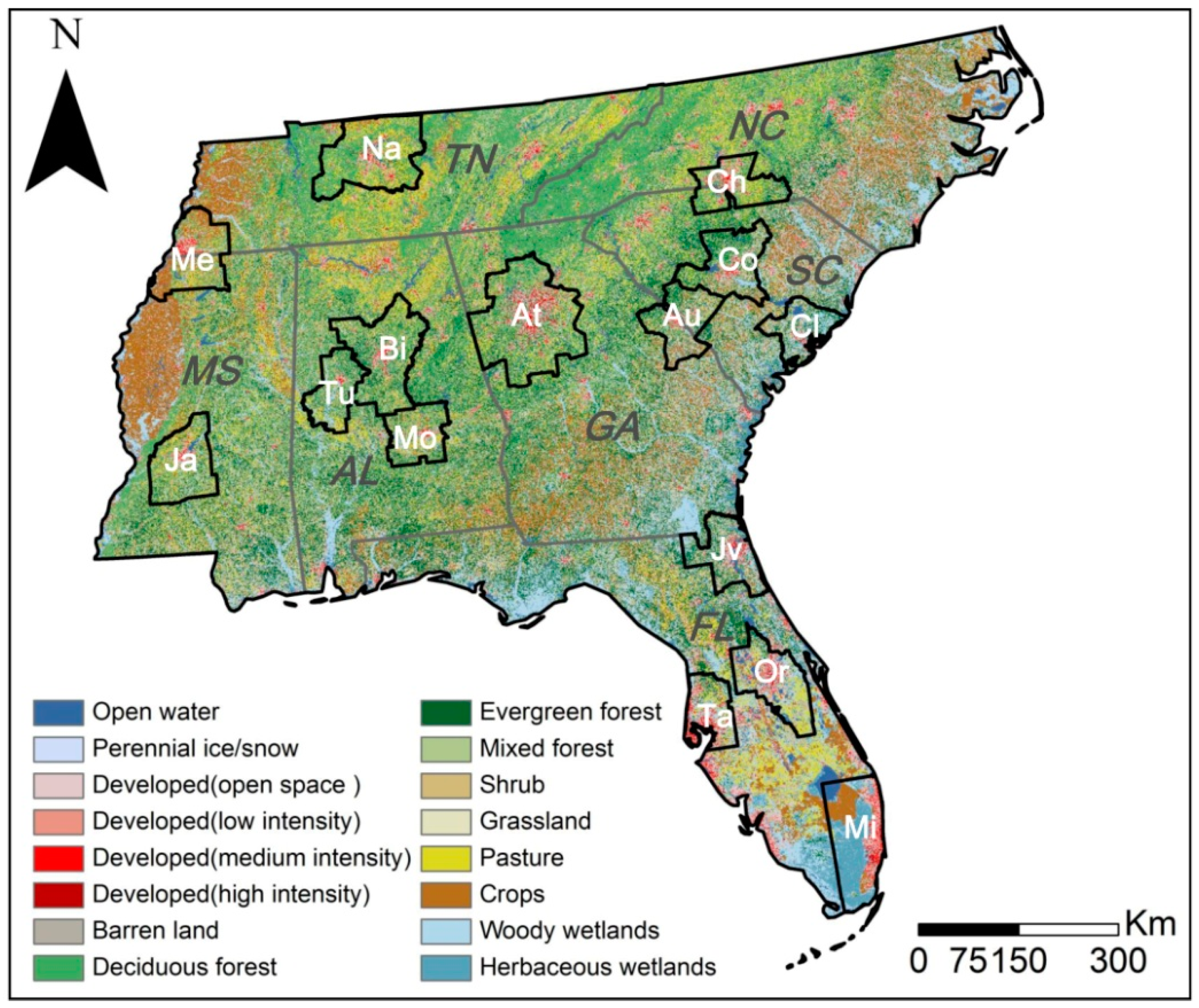
2.1. Study Area
2.2. Dataset
2.3. Methodology
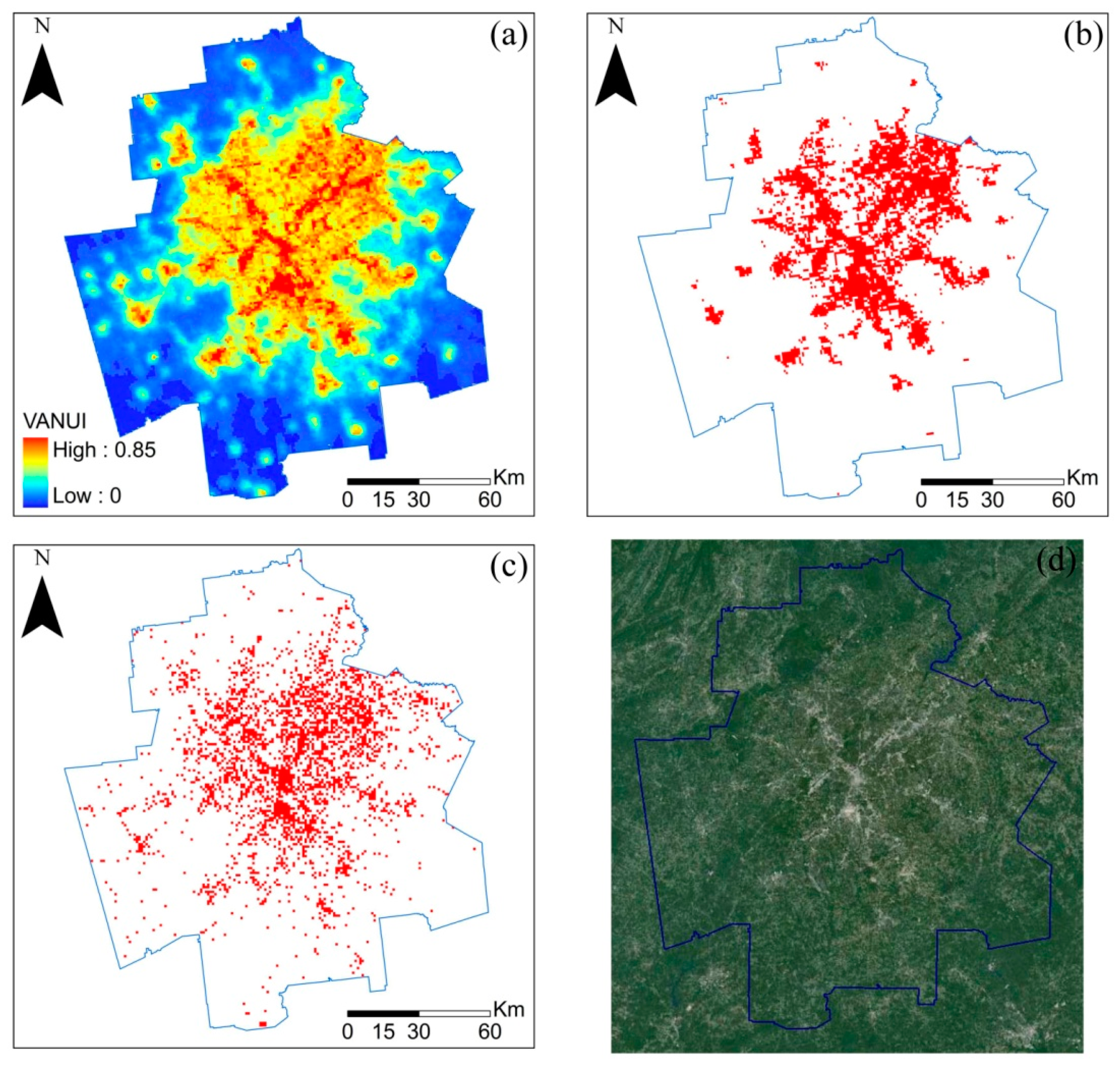
2.3.1. Urban Area Extraction from NTL Data
- Data inter-calibration
- VANUI calculation
- Generation of training samples and the calculation of thresholds
- Urban area detection
2.3.2. Built-Up Area Change Analysis
3. Results
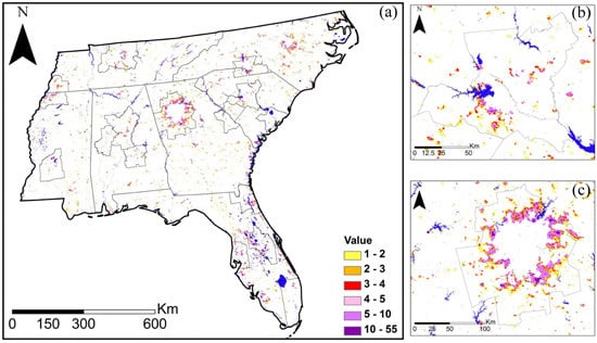
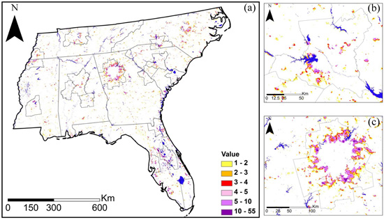
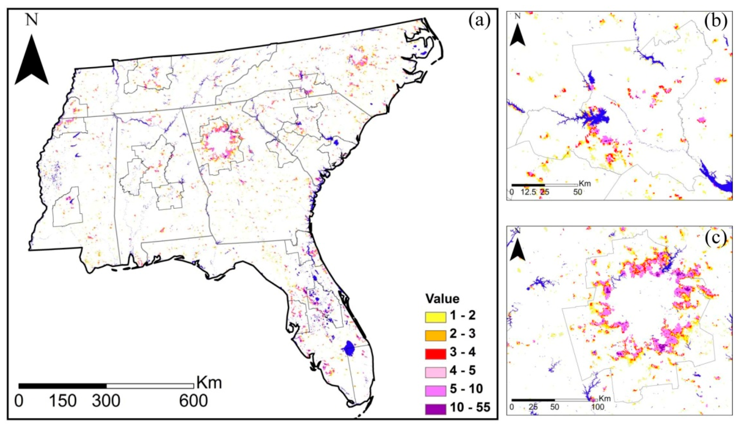
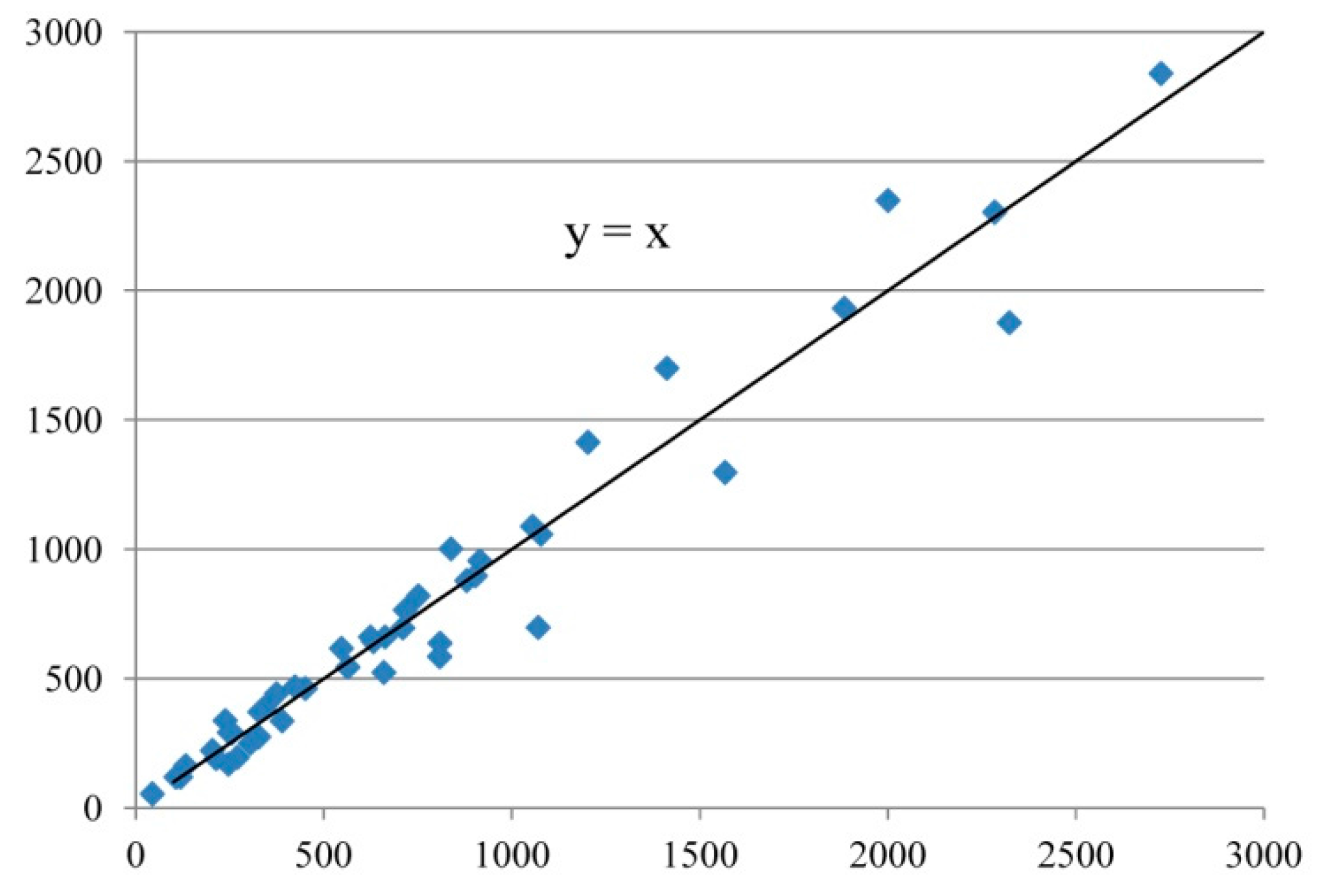
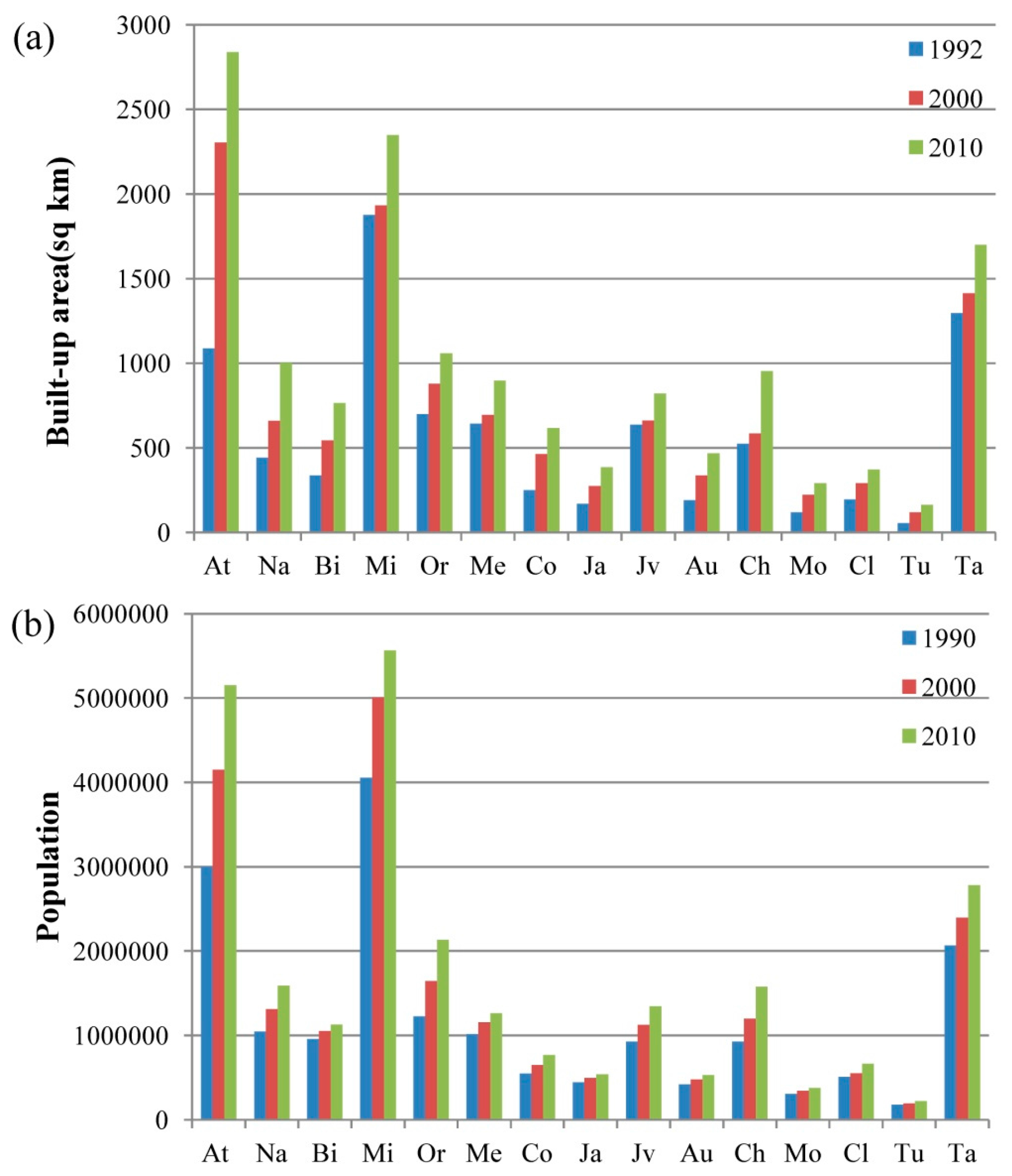
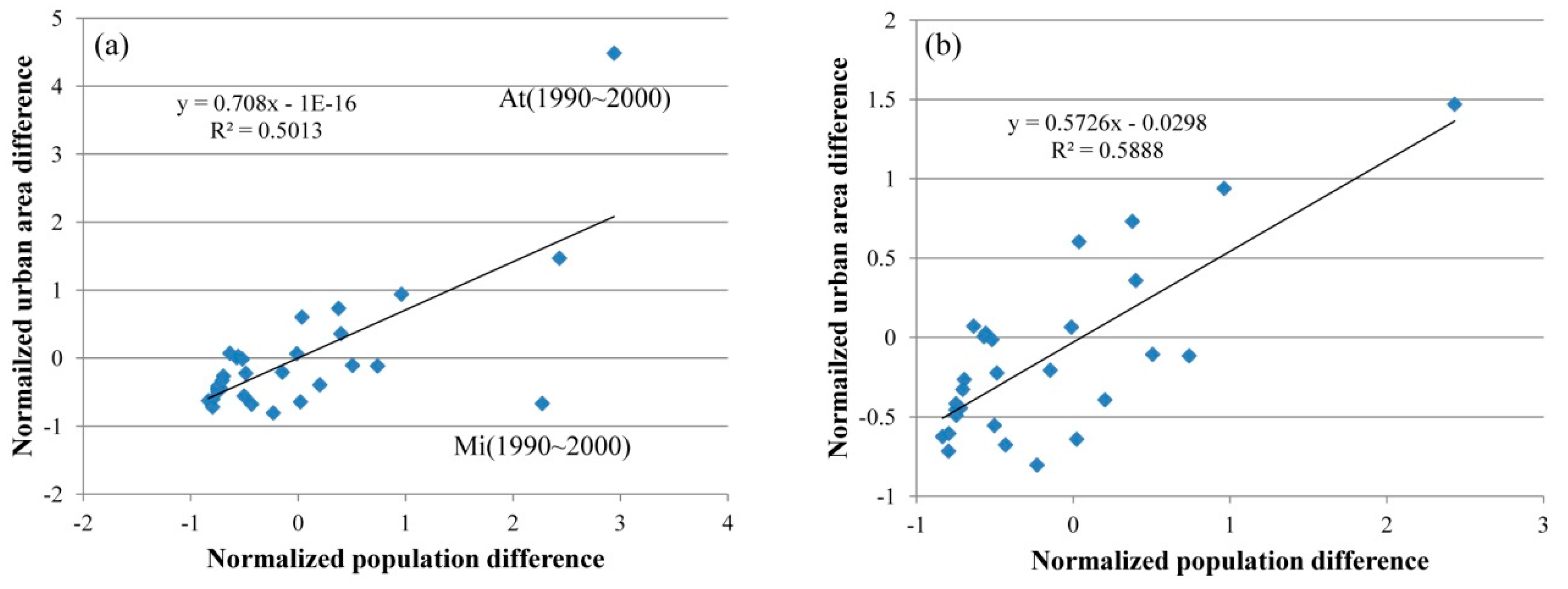
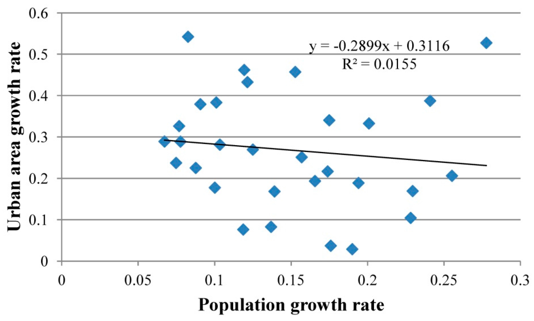
3.1. Regional Trend Analysis
3.2. Built-Up Area Detection and Accuracy Assessment
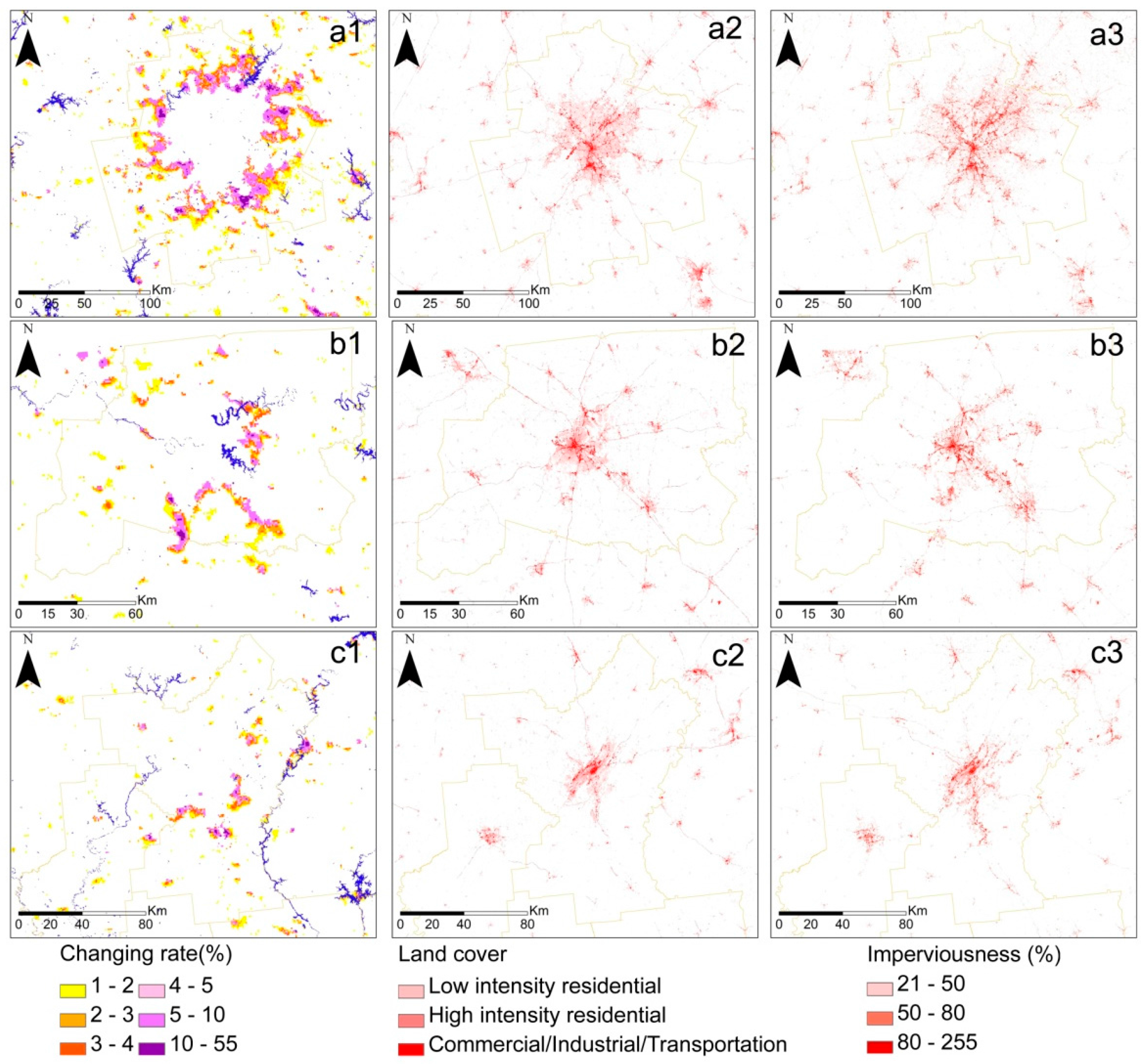
3.3. Spatiotemporal Patterns of Built-Up Area Changes in Metropolitan Areas
4. Discussion
5. Conclusions
Acknowledgments
Author Contributions
Conflicts of Interest
References
- Foley, J.A.; DeFries, R.; Asner, G.P.; Barford, C.; Bonan, G.; Carpenter, S.R.; Chapin, F.S.; Coe, M.T.; Daily, G.C.; Gibbs, H.K. Global consequences of land use. Science 2005, 309, 570–574. [Google Scholar] [CrossRef] [PubMed]
- Elvidge, C.D.; Baugh, K.E.; Dietz, J.B.; Bland, T.; Sutton, P.C.; Kroehl, H.W. Radiance calibration of DMSP-OLS low light imaging data of human settlements. Remote Sens. Environ. 1999, 68, 77–88. [Google Scholar] [CrossRef]
- Elvidge, C.D.; Baugh, K.E.; Kihn, E.A.; Kroehl, H.W.; Davis, E.R.; Davis, C.W. Relation between satellite observed visible-near infrared emissions, population, economic activity and electric power consumption. Int. J. Remote Sens. 1997, 18, 1373–1379. [Google Scholar] [CrossRef]
- Sutton, P.; Elvidge, C.; Obremski, T. Building and evaluating models to estimate ambient population density. Photogramm. Eng. Remote Sens. 2003, 69, 545–554. [Google Scholar] [CrossRef]
- Doll, C.; Muller, J.; Elvidge, C. Night-time imagery as a tool for global mapping of socioeconomic parameters and greenhouse gas emissions. Ambio 2000, 29, 157–162. [Google Scholar] [CrossRef]
- Xie, Y.; Weng, Q. World energy consumption pattern as revealed by DMSP-OLS nighttime light imagery. GISci. Remote Sens. 2016, 53, 265–282. [Google Scholar] [CrossRef]
- Elvidge, C.D.; Baugh, K.E.; Kihn, E.A.; Kroehl, H.W.; Davis, E.R. Mapping city lights with nighttime data from the DMSP Operational Linescan System. Photogramm. Eng. Remote Sens. 1997, 63, 727–734. [Google Scholar]
- Imhoff, M.L.; Lawrence, W.T.; Stutzer, D.C.; Elvidge, C.D. A technique for using composite DMSP-OLS “City Lights” satellite data to map urban area. Remote Sens. Environ. 1997, 61, 361–370. [Google Scholar] [CrossRef]
- Sutton, P.; Roberts, C.; Elvidge, C.; Meij, H. A comparison of nighttime satellite imagery and population density for the continental united states. Photogramm. Eng. Remote Sens. 1997, 63, 1303–1313. [Google Scholar]
- Sutton, P.; Roberts, D.; Elvidge, C.D.; Baugh, K. Census from heaven: An estimate of the global human population using night-time satellite imagery. Int. J. Remote Sens. 2001, 22, 3061–3076. [Google Scholar] [CrossRef]
- Small, C.; Pozzi, F.; Elvidge, C.D. Spatial analysis of global urban extent from DMSP-OLS night lights. Remote Sens. Environ. 2005, 96, 277–291. [Google Scholar] [CrossRef]
- Sutton, P.C.; Cova, T.J.; Elvidge, C.D. Mapping “Exurbia” in the conterminous United States using nighttime satellite imagery. Geocarto Int. 2006, 21, 39–45. [Google Scholar] [CrossRef]
- Henderson, M.; Yeh, E.T.; Gong, P.; Elvidge, C.; Baugh, K. Validation of urban boundaries derived from global night-time satellite imagery. Int. J. Remote Sens. 2003, 24, 595–609. [Google Scholar] [CrossRef]
- Milesi, C.; Elvidge, C.D.; Nemani, R.R.; Running, S.W. Assessing the impact of urban land development on net primary productivity in the southeastern United States. Remote Sens. Environ. 2003, 86, 401–410. [Google Scholar] [CrossRef]
- Liu, Z.; He, C.; Zhang, Q.; Huang, Q.; Yang, Y. Extracting the dynamics of urban expansion in China using DMSP-OLS nighttime light data from 1992 to 2008. Landsc. Urban Plan. 2012, 106, 62–72. [Google Scholar] [CrossRef]
- He, C.; Shi, P.; Li, J.; Chen, J.; Pan, Y.; Li, J.; Li, Z.; Toshiaki, I. Restoring urbanization process in China in the 1990s by using non-radiance-calibrated DMSP/OLS nighttime light imagery and statistical data. Chin. Sci. Bull. 2006, 51, 1614–1620. [Google Scholar] [CrossRef]
- Zhang, Q.; Seto, K.C. Mapping urbanization dynamics at regional and global scales using multi-temporal DMSP/OLS nighttime light data. Remote Sens. Environ. 2011, 115, 2320–2329. [Google Scholar] [CrossRef]
- Zhang, Q.; Schaaf, C.; Seto, K.C. The Vegetation Adjusted NTL Urban Index: A new approach to reduce saturation and increase variation in nighttime luminosity. Remote Sens. Environ. 2013, 129, 32–41. [Google Scholar] [CrossRef]
- Ma, Q.; He, C.; Wu, J.; Liu, Z.; Zhang, Q.; Sun, Z. Quantifying spatiotemporal patterns of urban impervious surfaces in China: An improved assessment using nighttime light data. Landsc. Urban Plan. 2014, 130, 36–49. [Google Scholar] [CrossRef]
- Shao, Z.; Liu, C. The integrated use of DMSP-OLS Nighttime Light and MODIS data for monitoring large-scale impervious surface dynamics: A case study in the Yangtze River Delta. Remote Sens. 2014, 6, 9359–9378. [Google Scholar] [CrossRef]
- United States Census 2010. Available online: http://www.census.gov/2010census/ (accessed on 15 March 2016).
- Kaza, N. The changing urban landscape of the continental United States. Landsc. Urban Plan. 2013, 110, 74–86. [Google Scholar] [CrossRef]
- Terando, A.J.; Costanza, J.; Belyea, C.; Dunn, R.R.; McKerrow, A.; Collazo, J.A. The southern megalopolis: Using the past to predict the future of urban sprawl in the Southeast U.S. PLoS ONE 2014, 9, e102261. [Google Scholar] [CrossRef] [PubMed]
- Elvidge, C.D.; Ziskin, D.; Baugh, K.E.; Tuttle, B.T.; Ghosh, T.; Pack, D.W.; Erwin, E.H.; Zhizhin, M. A fifteen year record of global natural gas flaring derived from satellite data. Energies 2009, 2, 595–622. [Google Scholar] [CrossRef]
- Huete, A.; Didan, K.; Miura, T.; Rodriguez, E.P.; Gao, X.; Ferreira, L.G. Overview of the radiometric and biophysic al performance of the MODIS vegetation indices. Remote Sens. Environ. 2002, 83, 195–213. [Google Scholar] [CrossRef]
- Homer, C.G.; Dewitz, J.A.; Yang, L.; Jin, S.; Danielson, P.; Xian, G.; Coulston, J.; Herold, N.D.; Wickham, J.D.; Megown, K. Completion of the 2011 National Land Cover Database for the conterminous United States-representing a decade of land cover change information. Photogramm. Eng. Remote Sens. 2015, 81, 345–354. [Google Scholar]
- Xian, G.; Homer, C.; Dewitz, J.; Fry, J.; Hossain, N.; Wickham, J. The change of impervious surface area between 2001 and 2006 in the conterminous United States. Photogramm. Eng. Remote Sens. 2011, 77, 758–762. [Google Scholar]
- Teillet, P.; Holben, B. Towards operational radiometric calibration of NOAA AVHRR imagery in the visible and near-infrared channels. Can. J. Remote Sens. 1994, 20, 1–10. [Google Scholar]
- Steven, M.D.; Malthus, T.J.; Baret, F.; Xu, H.; Chopping, M.J. Intercalibration of vegetation indices from different sensor systems. Remote Sens. Environ. 2003, 88, 412–422. [Google Scholar] [CrossRef]
- Weng, Q.; Lu, D. A sub-pixel analysis of urbanization effect on land surface temperature and its interplay with impervious surface and vegetation coverage in Indianapolis, United States. Int. J. Appl. Earth Obs. 2008, 10, 68–83. [Google Scholar] [CrossRef]
- Lu, D.; Tian, H.; Zhou, G.; Ge, H. Regional mapping of human settlements in southeastern China with multisensor remotely sensed data. Remote Sens. Environ. 2008, 112, 3668–3679. [Google Scholar] [CrossRef]
- Hirsch, R.M.; Slack, J.R. A nonparametric trend test for seasonal data with serial dependence. Water Resour. Res. 1984, 20, 727–732. [Google Scholar] [CrossRef]
- De Jong, R.; de Bruin, S.; de Wit, A.; Schaepman, M.E.; Dent, D.L. Analysis of monotonic greening and browning trends from global NDVI time-series. Remote Sens. Environ. 2011, 115, 692–702. [Google Scholar] [CrossRef] [Green Version]
- Fensholt, R.; Langanke, T.; Rasmussen, K.; Reenberg, A.; Prince, S.D.; Tucker, C.; Scholes, R.J.; Bao Le, Q.; Bondeau, A.; Eastman, R.; et al. Greenness in semi-arid areas across the globe 1981–2007—An Earth Observing Satellite based analysis of trends and drivers. Remote Sens. Environ. 2012, 121, 144–158. [Google Scholar]
- Cao, X.; Chen, J.; Imura, H.; Higashi, O. A SVM-based method to extract urban areas from DMSP-OLS and SPOT VGT data. Remote Sens. Environ. 2009, 113, 2205–2209. [Google Scholar] [CrossRef]
- Pandey, B.; Joshi, P.K.; Seto, K.C. Monitoring urbanization dynamics in India using DMSP/OLS night time lights and SPOT-VGT data. Int. J. Appl. Earth Obs. Geoinf. 2013, 23, 49–61. [Google Scholar] [CrossRef]
- Zhou, N.; Hubacek, K.; Roberts, M. Analysis of spatial patterns of urban growth across South Asia using DMSP-OLS nighttime lights data. Appl. Geogr. 2015, 63, 292–303. [Google Scholar] [CrossRef]
- Brueckner, J.K. Urban sprawl: Diagnosis and remedies. Int. Reg. Sci. Rev. 2000, 23, 160–171. [Google Scholar] [CrossRef]
- Zhou, Y.; Smith, S.J.; Elvidge, C.D.; Zhao, K.; Thomson, A.; Imhoff, M. A cluster-based method to map urban area from DMSP/OLS nightlights. Remote Sens. Environ. 2014, 147, 173–185. [Google Scholar] [CrossRef]
- Xiao, P.; Wang, X.; Feng, X.; Zhang, X.; Yang, Y. Detecting China’s urban expansion over the past three decades using nighttime light data. IEEE J. Sel. Top. Appl. 2014, 7, 4095–4106. [Google Scholar]
- Elvidge, C.D.; Baugh, K.E.; Zhizhin, M.; Hsu, F.C. Why VIIRS data are superior to DMSP for mapping nighttime lights. Proc. Asia Pac. Adv. Netw. 2013, 35, 62–69. [Google Scholar] [CrossRef]
- Coscieme, L.; Pulselli, F.M.; Bastianoni, S.; Elvidge, C.D.; Anderson, S.; Sutton, P.C. A thermodynamic geography: Night-time satellite imagery as a proxy measure of emergy. Ambio 2014, 43, 969–979. [Google Scholar] [CrossRef] [PubMed]
- Huang, X.; Schneider, A.; Friedl, M.A. Mapping sub-pixel urban expansion in China using MODIS and DMSP/OLS nighttime lights. Remote Sens. Environ. 2016, 175, 92–108. [Google Scholar] [CrossRef]
- Frolking, S.; Milliman, T.; Seto, K.C.; Friedl, M.A. A global fingerprint of macro-scale changes in urban structure from 1999 to 2009. Environ. Res. Lett. 2013, 8, 024004. [Google Scholar] [CrossRef]


| Metropolitan Area | Short Name | Area (sq km) |
|---|---|---|
| Atlanta-Sandy Springs-Marietta, GA | At | 21,965.8 |
| Nashville-Davidson-Murfreesboro-Franklin, TN | Na | 14,925 |
| Birmingham-Hoover, AL | Bi | 13,907.6 |
| Miami-Fort Lauderdale-Pompano Beach, FL | Mi | 13,823.1 |
| Orlando-Kissimmee-Sanford, FL | Or | 10,389.6 |
| Memphis, TN-MS-AR | Me | 10,382.8 |
| Columbia, SC | Co | 9930.07 |
| Jackson, MS | Ja | 9829.24 |
| Jacksonville, FL | Jv | 8740.09 |
| Augusta-Richmond County, GA-SC | Au | 8611.35 |
| Charlotte-Gastonia-Rock Hill, NC-SC | Ch | 8150.44 |
| Montgomery, AL | Mo | 7216.77 |
| Charleston-North Charleston-Summerville, SC | Cl | 6917.13 |
| Tuscaloosa, AL | Tu | 6909.29 |
| Tampa-St. Petersburg-Clearwater, FL | Ta | 6623.5 |
| Urban Area Class | Description |
|---|---|
| Developed, Low Intensity | Areas with a mixture of constructed materials and vegetation. Impervious surfaces account for 20%–49% percent of total cover. These areas most commonly include single-family housing units. |
| Developed, Medium Intensity | Areas with a mixture of constructed materials and vegetation. Impervious surfaces account for 50%–79% of the total cover. These areas most commonly include single-family housing units. |
| Developed, High Intensity | Highly developed areas where people reside or work in high numbers. Examples include apartment complexes, row houses and commercial/industrial. Impervious surfaces account for 80%–100% of the total cover. |
| Classification | Reference Data | User’s Accuracy (%) | ||
|---|---|---|---|---|
| Built-Up | Non Built-Up | Total | ||
| Built-up | 168 | 91 | 259 | 64.86 |
| Non Built-up | 70 | 742 | 812 | 91.38 |
| Total | 238 | 833 | 1071 | |
| Producer’s Accuracy (%) | 70.59 | 89.08 | 84.98 | |
© 2016 by the authors; licensee MDPI, Basel, Switzerland. This article is an open access article distributed under the terms and conditions of the Creative Commons Attribution (CC-BY) license (http://creativecommons.org/licenses/by/4.0/).
Share and Cite
Li, Q.; Lu, L.; Weng, Q.; Xie, Y.; Guo, H. Monitoring Urban Dynamics in the Southeast U.S.A. Using Time-Series DMSP/OLS Nightlight Imagery. Remote Sens. 2016, 8, 578. https://doi.org/10.3390/rs8070578
Li Q, Lu L, Weng Q, Xie Y, Guo H. Monitoring Urban Dynamics in the Southeast U.S.A. Using Time-Series DMSP/OLS Nightlight Imagery. Remote Sensing. 2016; 8(7):578. https://doi.org/10.3390/rs8070578
Chicago/Turabian StyleLi, Qingting, Linlin Lu, Qihao Weng, Yanhua Xie, and Huadong Guo. 2016. "Monitoring Urban Dynamics in the Southeast U.S.A. Using Time-Series DMSP/OLS Nightlight Imagery" Remote Sensing 8, no. 7: 578. https://doi.org/10.3390/rs8070578