Article

First Experiences in Mapping Lake Water Quality Parameters with Sentinel-2 MSI Imagery

1
Estonian Marine Institute, University of Tartu, Mäealuse 14, 12618 Tallinn, Estonia
2
Centre for Limnology, Estonian University of Life Sciences, Kreutzwaldi 5, 51014 Tartu, Estonia
*
Author to whom correspondence should be addressed.
Remote Sens. 2016, 8(8), 640; https://doi.org/10.3390/rs8080640
Submission received: 18 March 2016 / Revised: 10 July 2016 / Accepted: 1 August 2016 / Published: 5 August 2016

Abstract

:
The importance of lakes and reservoirs leads to the high need for monitoring lake water quality both at local and global scales. The aim of the study was to test suitability of Sentinel-2 Multispectral Imager’s (MSI) data for mapping different lake water quality parameters. In situ data of chlorophyll a (Chl a), water color, colored dissolved organic matter (CDOM) and dissolved organic carbon (DOC) from nine small and two large lakes were compared with band ratio algorithms derived from Sentinel-2 Level-1C and atmospherically corrected (Sen2cor) Level-2A images. The height of the 705 nm peak was used for estimating Chl a. The suitability of the commonly used green to red band ratio was tested for estimating the CDOM, DOC and water color. Concurrent reflectance measurements were not available. Therefore, we were not able to validate the performance of Sen2cor atmospheric correction available in the Sentinel-2 Toolbox. The shape and magnitude of water reflectance were consistent with our field measurements from previous years. However, the atmospheric correction reduced the correlation between the band ratio algorithms and water quality parameters indicating the need in better atmospheric correction. We were able to show that there is good correlation between band ratio algorithms calculated from Sentinel-2 MSI data and lake water parameters like Chl a (R2 = 0.83), CDOM (R2 = 0.72) and DOC (R2 = 0.92) concentrations as well as water color (R2 = 0.52). The in situ dataset was limited in number, but covered a reasonably wide range of optical water properties. These preliminary results allow us to assume that Sentinel-2 will be a valuable tool for lake monitoring and research, especially taking into account that the data will be available routinely for many years, the imagery will be frequent, and free of charge.

Graphical Abstract

1. Introduction

Lakes and reservoirs act as regulators of carbon cycling and climate [1]. They provide water for multiple human uses from drinking water to recreation and support high levels of biodiversity [2]. There is a high need for monitoring lake water quality at local to global scales. There are about 117 million lakes in the world [3], but only a small fraction of them is included in in situ monitoring networks and the frequency of in situ monitoring is often limited. Increasing amount of lakes has been equipped with automated monitoring systems [4,5] that provided data with sufficient frequency. However, the number of lakes with such systems is still rather small. Satellite remote sensing is the only feasible way to monitor lakes when we have global questions (like carbon cycle) under investigation, or when water quality over large regions has to be monitored with reasonable frequency.
Water quality indicators like chlorophyll a (Chl a), total suspended matter, turbidity, Secchi depth and colored dissolved organic matter (CDOM) can be measured using remote sensing techniques [6,7,8,9,10,11,12,13]. In our study, we concentrated on the Chl a, CDOM and its related parameters like dissolved organic carbon (DOC) and water color. The photosynthetic pigment Chl a is a key indicator of phytoplankton biomass. Thus, the estimation of Chl a concentration is essential for monitoring of water quality [14]. CDOM and DOC are also of great interest playing a significant role in the carbon and energy cycle of lakes and affecting treatability of drinking water [15,16].
Satellite monitoring of lakes has been hampered by lack of appropriate satellite sensors [17]. Ocean color sensors, like the Moderate Resolution Imaging Spectroradiometer (MODIS) and the MEdium Resolution Imagining Spectrometer, (MERIS), had frequent revisit time (1–3 days) and sufficient radiometric resolution (12-bit) needed for dark objects like waterbodies. However, spatial resolution of these sensors (300–1000 m) was suitable only for very large lakes while majority of the lakes on Earth are small [3]. Previous Landsat series (Landsat 1–7) satellites had good spatial resolution (30–79 m) but limited radiometric resolution (6–8 bits) being usable to certain extent for mapping lake water quality parameters [8,13,18,19,20]. Landsat 8 radiometric resolution is 12-bit and it is suitable for remote sensing of even dark (CDOM-rich) lakes [21]. Still, the revisit time of Landsat 8 is rather long (16 days) limiting its use in routine monitoring of lake water quality.
The launch of Multispectral Imager’s (MSI) onboard Sentinel-2 in 2015 opened a great new potential in lake remote sensing. The imagery is with 10 m, 20 m and 60 m spatial resolution, meaning that even small lakes can be studied. Data are acquired in 13 spectral bands and radiometric resolution of the sensor is 12-bit [22]. Revisit time of Sentinel-2 will be five days when the second satellite is in orbit in the beginning of 2017. However, at higher latitudes, like in Estonia, the revisit time will be almost every second day because of the overlapping orbits.
The MSI was not designed for aquatic remote sensing. Up to now the usefulness of the MSI for water applications has been demonstrated only for separating water bodies from land [23]. Mapping water bodies from space using MSI data should allow improving the global inland water map from current 14.25 m resolution [3] to 10 m. Frequent high spatial resolution imagery will allow also to move from static inland water maps to dynamic ones, i.e., separate “permanent” inland waters from temporarily inundated areas. Hedley et al. [24] demonstrated with synthetic dataset that the MSI data are potentially useful for coral reef mapping and detecting bleaching events. However, coral reefs are relatively bright objects while lakes in boreal zone are relatively dark making retrieval of water quality parameters a more demanding task. We have shown earlier [21] that the Sentinel-2 spectral band at 783 nm can detect part of the signal of the 810 nm peak [21]. In the extreme CDOM-rich lakes, this peak is the only piece of information not affected by CDOM absorption and can be used for estimating concentration of Chl a. However, this study was mainly performed using hyperspectral field data and the performance of MSI was demonstrated only at qualitative bases. Therefore, there is currently no demonstration that the MSI imagery can be used for mapping inland water quality.
Atmospheric correction of inland water imagery is a complicated issue. Some authors [19,20] have even shown for Landsat imagery that the top of atmosphere imagery provided better result than atmospherically corrected imagery. The Sentinel-2 toolbox contains Sen2cor atmospheric correction procedure. It was not designed for waterbodies. However, it will probably be the first choice for many users due to its availability in the toolbox. We do not have in situ measured reflectance data collected simultaneously with Sentinel-2 overpass. Therefore, it was not possible to validate the performance of Sen2cor directly.
The main aim of our study was to test suitability of Sentinel-2 MSI data for mapping different lake water quality parameters (Chl a, water color, CDOM and DOC) by means of band ratio type algorithms, which have demonstrated good performance in previous lake remote sensing studies using other multispectral sensors. We assume that this will be a demonstration of the suitability of the Sentinel-2 MSI sensor for quantitative lake remote sensing if the algorithms that performed well in the case of other sensors perform well also in the case of MSI.

2. Materials and Methods

2.1. Study Sites and in Situ Data

Nine small and two large lakes (Lake Peipsi and Lake Võrtsjärv) were sampled in the frame of the state monitoring program in Estonia, August 2015. All lakes were sampled once. The locations of the studied lakes are shown in Figure 1. There were 8 sampling points in Lake Võrtsjärv, 6 in Lake Peipsi and one in each small lake (altogether 23 sampling points). More detailed information about sampled lakes is displayed in Table 1.
In situ data were collected from 3 August 2015 to 18 August 2015. The mean time difference between Sentinel-2 and in situ data were approximately 5 days. DOC, CDOM, water color and Chl a were measured from surface (small lakes) or from integrated water samples (large lakes). No in situ reflectance measurements were carried out during this field campaign.
For the determination of DOC concentrations (mg·L−1) in small lakes, water samples were filtered through Whatman GF/F glass microfiber filters previously washed with 500 mL of ultrapure water (Milli-Q) and the organic carbon content of the filtrates were measured by a TOC-VCPH analyzer (Shimadzu, Kyoto, Japan). This method conforms to the European standard method [25]. DOC concentrations were determined directly as inorganic carbon was eliminated by acidifying samples to pH 2 or less with 2 M HCl and subsequently purging samples with purified gas to remove the CO2. The samples were combusted at 680 °C to convert DOC components to CO2 which was detected with a non-dispersed infrared gas analyzer. For determination of DOC concentrations in Lakes Peipsi and Võrtsjärv, the carbon content of the filtrate was measured according to [26].
The amount of CDOM was characterized by its concentration (mg·L−1) calculated from following equation [27,28]:
C C D O M = c* f ( λ ) exp ( S ( λ λ 0 ) ) a* C D O M ( λ 0 )
where a*CDOM0) is the specific absorption coefficient of DOM, which numerical value at λ0 = 380 nm was 0.565 L·m−1·mg−1 [27]; S is the slope parameter equal to 0.017 nm−1 [28]; and c*f(λ) was taken from spectrometric reading at λ = 380 nm.
Water color is usually routinely analyzed water quality parameter in limnological studies, but also in water treatment plants, since it can be measured easily and at minimal cost. Water color is measured from filtered water and it gives us similar information about water quality as DOC and CDOM, but it is much more robust. Water color (mg·Pt·L−1) was determined by spectrophotometric measurements of absorbance at 410 nm in Lake Peipsi and Võrtsjärv and at 420 nm in small lakes in our study. Both methods conform to the ISO standard method [29].
For Chl a (µg·L−1), 0.1–1 L of water was passed through Whatman GF/F glass microfiber filter and concentrations were measured spectrophotometrically [30] at a wavelength of 665 nm from 96% ethanol extracts of the filters.

2.2. Sentinel-2 Data

Sentinel-2 Level-1C (L1C) MSI data were downloaded from Sentinels Scientific Data Hub (https://scihub.copernicus.eu/). Sentinel-2 images were available on 11, 14 and 17 August 2015. The L1C product is composed of 100 km2 tiles (ortho-images in UTM/WGS84 projection) [22]. Per-pixel radiometric measurements are provided in Top of Atmosphere (TOA) reflectances with all parameters to transform them into radiances. L1C products are resampled with a constant Ground Sampling Distance (GSD) of 10, 20 and 60 m depending on the native resolution of the different spectral bands (Table 2) [22]. The images from WGS84 UTM zone 35 with 20 m resolution were used.
Sentinel-2 Toolbox (S2TBX) version 2.0.4 in Sentinel Application Platform (SNAP) version 2.0.2 on Windows 7 (64 bit) was used to process the images. Then, 3 × 3 cloud free pixels were extracted from each sampling point situated in the middle of the lake and the mean values of the pixels were used for analyses. To get the Level-2A (L2A) Bottom of Atmosphere (BOA) reflectance images (derived from the associated L1C products) Sen2cor atmospheric correction module was applied.

2.3. Remote Sensing Algorithms

As was mentioned above, our aim was not developing new remote sensing algorithm but to test the performance of MSI with well-established band ratio algorithms that have performed well in the case of other sensors. The height of the reflectance peak between 700 and 720 nm has been used for estimating the Chl a concentration in lake waters for more than two decades [6,31,32,33,34]. Sentinel-2 has band 5 (705 nm) in this spectral region. Therefore, we calculated the height of the peak against the band 4 (665 nm) and band 6 (740 nm) baselines and tested whether it is in correlation with the chlorophyll a in the studied lakes.
CDOM absorption is the strongest in the blue part of spectrum and decreases exponentially with increasing wavelength. Therefore, it would be logical to use blue to red ratios for estimating lake CDOM content. However, water leaving signal in blue bands is often negligible in the case of lake waters due to CDOM and relatively high amount of phytoplankton that both absorb light in blue part of spectrum. In extreme CDOM-rich lakes the water leaving signal may be close to zero even in green and red parts of spectrum (up to 650 nm) [21]. However, if to exclude the extreme lakes then the green to red band ratios have demonstrated the best performance in retrieving lake CDOM from remote sensing [18,35,36,37]. It must be noted that the study by Zhu et al. [37] tested many algorithms with lake data from around the world and showed good performance of the green to red ratio globally. Therefore, we used the band 3 to band 4 ratio for estimating CDOM concentration from Sentinel-2 imagery. DOC concentration is in good correlation with its colored component CDOM in many lakes [38,39]. Thus, the same band ratio is used for retrieving lake DOC. In addition, we used the same band ratio for water color that is very similar parameter to CDOM.

3. Results

3.1. In Situ Data

The concentration of DOC varied from 6.04 to 20.9 mg·L−1, Chl a from 3.6 to 72.9 μg·L−1, CDOM from 1.77 to 15.8 mg·L−1 and water color from 3 to 30 mg·Pt·L−1 in studied lakes (Table 3). The highest values of Chl a, DOC, CDOM and water color were measured from Lake Lohja and Lake Võrtsjärv and the lowest from Lake Nohipalo Valgõjärv, Lake Rõuge Suurjärv and Lake Viitna Pikkjärv. DOC were measured only in one sampling point in Lake Võrtsjärv and in two sampling points in Lake Peipsi. Data collected on previous years have shown that the concentration of the DOC varies approximately 1–2 mg·L−1 between sampling points in those lakes [17]. There were no data about CDOM in Lake Peipsi in August 2015. The values of CDOM in Lake Peipsi have been similar to the values of CDOM measured from Lake Võrtsjärv in previous years [40].

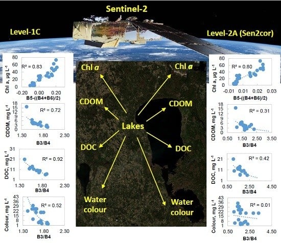
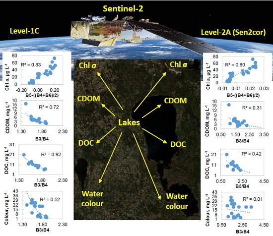
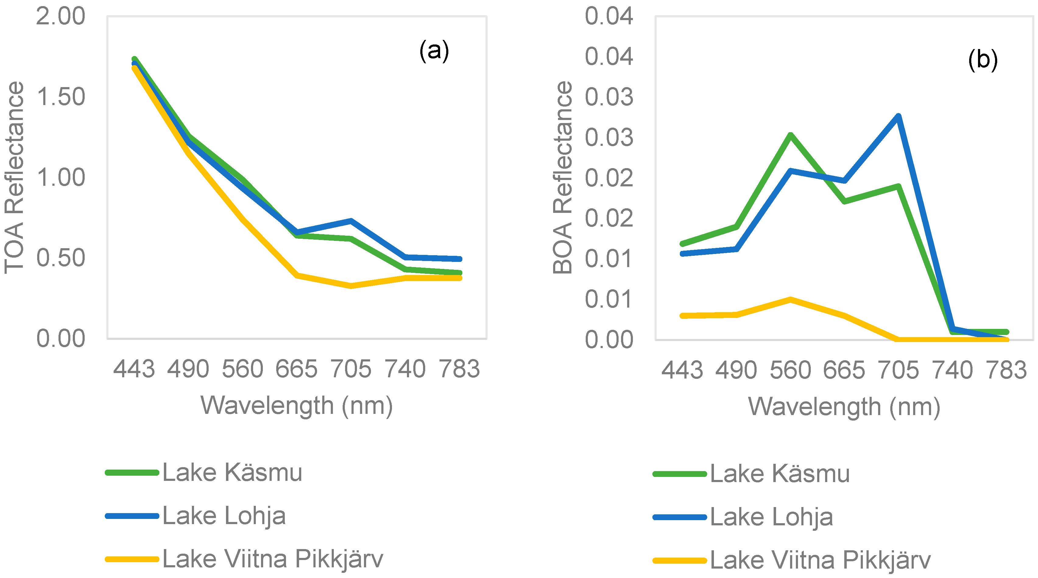
3.2. Atmospheric Correction and Reflectance Spectra

Sen2cor atmospheric correction procedure was used to remove atmospheric contribution from the MSI imagery. This procedure is not designed for aquatic environments. However, due to its availability in the Sentinel-2 Toolbox it will most probably be the first choice atmospheric correction procedure many people will use.
We do not have in situ reflectance measurements from the lakes under investigation carried out simultaneously with the Sentinel-2 overpass. Therefore, we cannot validate the performance of atmospheric correction directly. However, we have field reflectance data from Lakes Võrtsjärv and Peipsi collected in 2011–2013. These reflectance spectra were recalculated into Sentinel-2 bandwidths and compared with the Sen2cor corrected reflectances. This comparison is a good preliminary test of any atmospheric correction procedure as quite often the atmospheric correction procedures that perform well in the case of clear oceanic waters overcorrect the data in coastal and inland waters producing negative reflectances in blue part of spectrum. Sometimes the reflectance values are also negative at higher wavelengths. This did not happen in the case of Sen2cor and Sentinel-2 data, as seen in Figure 2. The atmospheric correction worked better in the case of Võrtsjärv where the Sentinel-2 reflectances resemble the in situ results well (Figure 2a). There are larger differences between Sentinel-2 and in situ measured reflectances in the case of Lake Peipsi data (Figure 2b).
Top of atmosphere (TOA) and bottom of atmosphere (BOA) reflectance spectra for selected lakes are shown in Figure 3 and Figure 4. The difference in optical properties of the studied lakes is clearly seen also in the reflectance spectra. For example, Viitna Pikkjärv has relatively clear water with low Chl a concentration. Its reflectance is the lowest and there is no peak at 705 nm typical to phytoplankton-rich waters. Lake Peipsi has relatively dark (CDOM-rich) waters while Lake Võrtsjärv is known by high amount of resuspended sediments due to its shallow water depth. The differences are clearly seen in Figure 4 where Lake Peipsi reflectance is much lower due to the higher absorption and smaller backscattering coefficient of its waters.

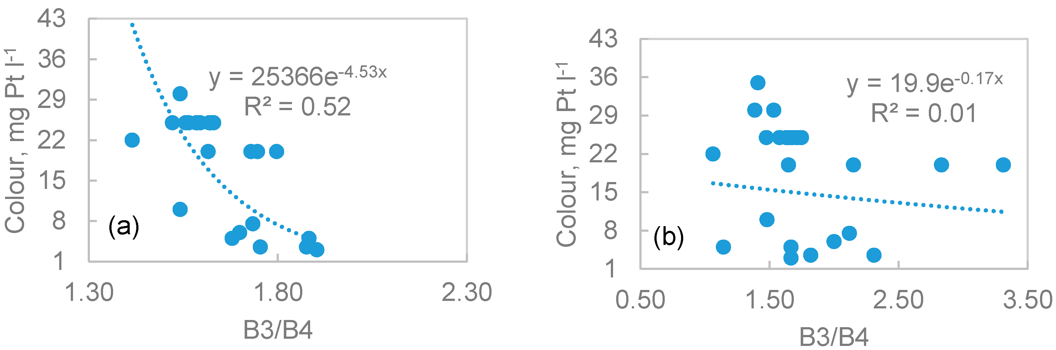
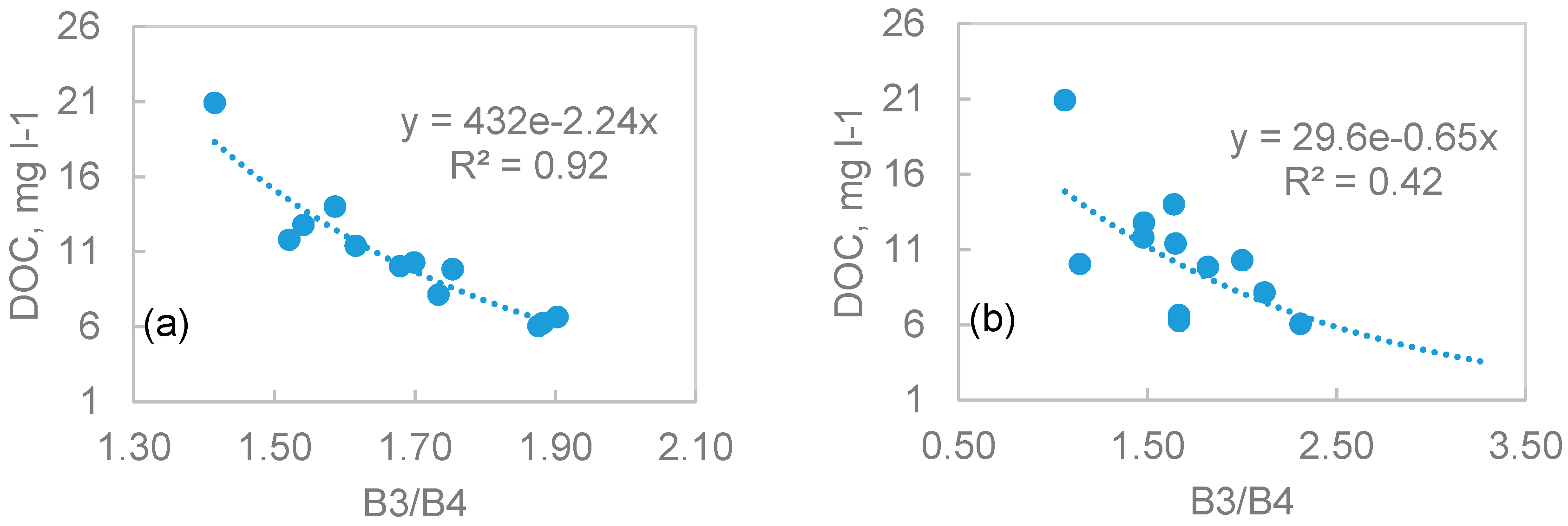
3.3. Results of the Remote Sensing Algorithms vs. in Situ Data

An algorithm describing the height of the 705 nm peak against the baseline of two neighboring spectral bands was used for chlorophyll retrieval (Figure 5).
There are several band ratio algorithms developed for estimating lake CDOM concentrations and closely related water color and DOC concentrations [18,35,36,37]. Most of them are based on the green to red ratio as water leaving signal is often very low in blue part of spectrum and atmospheric correction issues are usually the largest in the blue bands as well. Zhu et al. [37] have analyzed the performance of different CDOM-retrieval algorithms and found the green to red band ratio working well over wide variety of lakes in different part of the world. Therefore, we used also the MSI band 3 to band 4 ratio to retrieve CDOM, color and DOC concentrations (Figure 6, Figure 7 and Figure 8). Surprisingly, the correlation was the strongest with the DOC rather than the CDOM and water color that have direct effect on the water reflectance spectra. One of the possible explanations may be slightly different sets of lakes that were used in the analysis (see Table 3) as for some lakes from where we have DOC results CDOM was not measured and vice versa.

4. Discussion

The small (10 m) pixel size of the Sentinel-2 MSI sensor is a great advantage in lake remote sensing as even very small lakes can be observed. However, several critical for lake remote sensing bands (5–7) are available with 20 m resolution. To make use of the full spectral resolution between 443 and 783 nm, we resampled MSI spectral bands 1–7 to a common 20 m pixel size. In order to reduce the random noise we used an average of 3 × 3 pixels around the in-situ sampling points instead of the single pixel value. We studied lakes as small as 7 ha, but much smaller lakes can be studied with 20 m pixel size. This opens great potential for monitoring of water quality on regional to national scale or determining the role of lakes in the global carbon cycle where the small lakes are of greater importance due to their large number [3] and higher carbon sequestration [1].
The Sentinel-2 data used were collected on 11, 14, and 17 August 2015 while the in situ sampling was carried out during the period between August 3 and August 18. Studies in boreal lakes [20,41] have shown that a few days difference between the image acquisition and in situ data collection does not affect retrieval accuracy of water parameters significantly, especially in the case of relatively stable parameters like CDOM, DOC and water color. Kutser [20] found that ±3 days was as good as exact match-up, a week time difference reduced the correlation, but a month time difference was too much even for estimating a relatively stable parameter like CDOM. On the other hand Cardille et al. [41] found that even much longer time differences are still acceptable.
Water parameters can change over a short period mainly in two cases: heavy rain bringing dissolved and particulate material into the lakes or during phytoplankton blooms. Especially cyanobacterial blooms may be spatially very heterogeneous and biomass may vary two to three orders of magnitude within a few hundred meters. It has even been shown that 30 m pixel is not sufficient to describe the spatial variability of biomass in cyanobacterial blooms [42]. Weather conditions were stable between the image acquisition and in situ sampling and no cyanobacterial blooms were reported. One may assume that the time difference between the in situ sampling and image acquisition reduces the correlation between satellite products and the actual in situ values. This may have been the case also in our study, but the correlation coefficients were still very high indicating that the time difference was not a major problem.
Atmospheric correction of coastal and inland water imagery is a challenge. There are advancements also in atmospheric correction methods for optically complex waters [43,44]. Some of these procedures will become freely available and/or will be included in SNAP in the not so distant future. However, Sen2cor, freely available in the SNAP software, will probably be the first choice for many users to test. We were not able to validate the performance of Sen2cor in lake remote sensing directly as we did not have field reflectance data measured simultaneously with Sentinel-2 image acquisition. Consequently, we were able to assess the performance of the Sen2cor in two indirect ways—by comparing the reflectance spectra with our field data from the same lakes collected in previous years and by comparing the water parameter retrievals from corrected and uncorrected data. Based on the comparison of reflectance spectra we can see that the atmospheric correction worked better in the case of more turbid (higher signal) Lake Võrtsjärv. Lake Peipsi is more CDOM-rich with low reflectance in general and nearly negligible reflectance in blue part of spectrum. Sen2cor produced too high values in blue part of spectrum. This may be due to glint or atmospheric correction errors that are more pronounced in the case of low water leaving signal. The errors in blue part of spectrum are typical to all atmospheric correction procedures.
Reflectance spectra obtained for small lakes were also realistic. Therefore, we expected to see good performance of the remote sensing algorithms when atmospherically corrected data was used. Nevertheless, the results obtained with TOA reflectance were better than with BOA reflectance in the case of all studied parameters. In the case of chlorophyll a the difference was minor, but for other parameters it was relatively large. This indicates poor performance of Sen2cor in correcting lake pixels.
The location of the reflectance peak in the 700–720 nm region shifts towards longer wavelength with increasing concentration of phytoplankton. The Sentinel-2 MSI 705 nm band is almost perfectly located to capture this peak. Our results showed that the amplitude of the 705 nm peak against the 665–740 nm baseline was in very good correlation with Chl a concentration in the studied lakes (R2 = 0.83). In the case of Chl a estimation the atmospherically corrected data produced similar results with the TOA reflectance. This can be explained by the wavelengths used in the chlorophyll retrieval algorithm (longer wavelengths are less affected by atmospheric correction errors) and the type of algorithm that calculates the height of the 705 nm peak against a baseline. The performance of this kind of algorithms depends more on spectral shape rather than absolute values.
The commonly used [18,35,36,37] green to red band ratio was in good correlation with lake CDOM (R2 = 0.72) and water color (R2 = 0.52). Consequently, these lake parameters can be mapped from space using Sentinel-2 data. Surprisingly, the correlation with DOC was even higher (R2 = 0.92) than with CDOM. If in many lakes the correlation between DOC and its colored component is very strong [38,45,46] then in Estonian lakes the relationship is varying seasonally [47,48]. Moreover, it has been shown [49] that iron bound to carbon molecules absorbs light in a similar way like CDOM and variable carbon to iron ratio makes remote sensing mapping of lake DOC more complicated. One of the possible reasons of this result is slightly different set of lakes used as for some lakes from where we have DOC data CDOM was unavailable and vice versa. Another possible explanation is that the ratio of colored to uncolored DOC as well as carbon to iron ratio in the studied lakes somehow compensated each other’s optical effects and the green to red band ratio allows to predict lake DOC with higher confidence than CDOM.
The Chl a retrieval algorithm performed similarly well in the case of TOA and BOA reflectance spectra. However, the green to red ratio, used for retrieving CDOM, DOC and water color, performed much better in the case of TOA reflectance rather than from atmospherically corrected data. Atmospheric effects in the measured signal are the highest in blue end of spectrum and decrease nearly exponentially with increasing wavelength. The red and NIR bands are relatively little affected by the atmospheric effects. The green band, on the other hand, is affected by atmosphere much more. It is easy to understand that a minor error in atmospheric correction may be as large as the whole water leaving signal if more than 90% of the signal measured at the satellite altitude is atmospheric contribution. Therefore, the over- or undercorrection of the data is larger in the green band than in red and NIR bands and consequently minor errors in the atmospheric correction affect the CDOM/DOC retrieval algorithms much more than the Chl a retrieval algorithm based on the peak of the 705 nm band. This may be the reason why TOA reflectance gave better results than the BOA reflectance although the qualitative inspection of BOA reflectances showed that the water reflectances were reasonable for many lakes.
In the absence of better sensors for inland water remote sensing scientists have used land remote sensing satellites like Landsat or EO-1 (Advanced Land Imager and Hyperion) [8,9,13,18,19,20,35,36,37,41,47,50,51]. EO-1 was an experimental satellite and did not have global coverage. Landsat series satellites revisit time is 16 days. Meaning that monitoring of inland water quality was not possible as many processes (like algal blooms) may last shorter period than the 16 days and remain undetected with Landsat even in the lucky case where consecutive images are acquired in cloud free days. The situation will change dramatically when both Sentinel-2A and Sentinel-2B will be in orbit. Five days revisit time on the Equator and more frequent sampling at higher latitudes will make Sentinel-2 a real monitoring tool for inland and coastal waters where 300 m spatial resolution of OLCI (launched on Sentinel-3) is not sufficient. Moreover, combining the two Sentinel-2 with Landsat 8 will allow increasing the frequency of measurements even further. This is especially true for parameters like CDOM and DOC that can be estimated using green and red spectral bands that are rather similar on both sensors. Most probably this will also apply for total suspended solids (TSS). We did not have TSS data to test this with Sentinel-2, but usually TSS is the easiest parameter to estimate from satellites and for Landsat it was demonstrated already a quarter of the century ago [8]. Where significant advancement in lake and inland water remote sensing are foreseen after the launch of Sentinel-2 is remote sensing of Chl a. Landsat series satellites do not have spectral bands in the 700–720 nm spectral range. It has been demonstrated in many studies [6,10,11,21,31,32,33,34,42] that this peak is the best indicator of phytoplankton biomass and can be calculated from TOA data [33,34]. We found also that there is very good correlation between the peak height at 705 nm and chlorophyll concentration in the lakes and the relationship is relatively insensitive to atmospheric correction issues as the correlation was good both for TOA and BOA data.
The only problems in quantitative monitoring of phytoplankton biomass may occur when surface scum is formed during cyanobacterial blooms. First of all the thickness of the scum is usually unknown and its optical properties on the surface (seen by remote sensing sensors) may be quite different from the interior due to photobleaching and/or degradation of biomass. Moreover, we have shown in the case of cyanobacterial bloom in the Baltic Sea [52] that the 10 m spatial resolution of MSI is not sufficient in many circumstances as the stripes of scum at the surface may be too narrow. In such cases the reflectance of surface scum is identical to dense subsurface bloom and high NIR reflectance typical to floating biomass is not formed.

5. Conclusions

We did not have simultaneous field radiometry data to validate the performance of Sen2cor atmospheric correction directly. Comparison of the BOA reflectance with older field data showed that results are realistic in the case of more turbid lakes and not so good in the case of darker lakes. Comparing the results of water quality parameter retrieval from TOA and BOA imagery shows that the Sen2cor atmospheric correction did not perform well as the results are better for uncorrected data.
The results show that Sentinel-2 MSI data has great potential for inland water remote sensing as we were able to map Chl a, CDOM and DOC concentrations as well as water color in lakes by means of commonly used band ratio type algorithms.
This study is the first attempt to test capabilities of Sentinel 2 MSI sensor in inland water remote sensing. The results may be considered as preliminary because the in situ database was limited and no reflectance data was collected to validate the performance of atmospheric correction. Nevertheless, the results are very encouraging for inland water monitoring and research.

Acknowledgments

The study was funded by the Estonian Ministry of Education and Research (IUT 21-02, SF0180009s11, and PUT777), Estonian Science Foundation (grant 9102), EU FP7 project “Global Earth Observation for Integrated Water Resource Assessment—eartH2Observe, and Swiss Grant for Programme “Enhancing public environmental monitoring capacities”. The Estonian Ministry of Environment and Estonian Environment Agency supported data collection in the state monitoring programs. We are grateful to Malle Viik, Evi Lill and Katrin Ott for their help with the laboratory analyses. We are grateful to six anonymous reviewers and the editor for their comments, which greatly improved the manuscript.

Author Contributions

Kaire Toming was responsible for processing and analyzing Sentinel-2 imagery and, together with Tiit Kutser, wrote the bulk of the manuscript with input from all co-authors; Alo Laas provided in situ data and enhanced the manuscript; Margot Sepp participated in the fieldwork and carried out laboratory analysis of dissolved organic carbon, colored dissolved organic matter and water color; Birgot Paavel measured, processed and analyzed field reflectance data; and Tiina Nõges enhanced the manuscript.

Conflicts of Interest

The authors declare no conflict of interest.

References

  1. Tranvik, L.J.; Downing, J.A.; Cotner, J.B.; Loiselle, S.A.; Striegl, R.G.; Ballatore, T.J.; Dillon, P.; Knoll, L.B.; Kutser, T.; Larsen, S.; et al. Lakes and reservoirs as regulators of carbon cycling and climate. Limn. Oceanogr. 2009, 56, 2298–2314. [Google Scholar] [CrossRef]
  2. Brönmark, C.; Hansson, L.A. Environmental issues in lakes and ponds: Current state and perspectives. Environ. Conserv. 2002, 29, 290–307. [Google Scholar] [CrossRef]
  3. Verpoorter, C.; Kutser, T.; Seekel, D.; Tranvik, L.J. A global inventory of lakes based on high-resolution satellite imagery. Geophys. Res. Lett. 2014, 41, 639–642. [Google Scholar] [CrossRef]
  4. Staehr, P.A.; Baastrup-Spohr, L.; Sand-Jensen, K.; Stedmon, C. Lake metabolism scales with lake morphometry and catchment conditions. Aquat. Sci. 2012, 74, 155–169. [Google Scholar] [CrossRef]
  5. Meinson, P.; Idrizaj, A.; Nõges, P.; Nõges, T.; Laas, A. Continuous and high-frequency measurement in limnology: History, applications, and future challenges. Environ. Rev. 2016, 24, 1–11. [Google Scholar] [CrossRef]
  6. Kallio, K.; Kutser, T.; Hannonen, T.; Koponen, S.; Pulliainen, J.; Vepsälainen, J.; Pyhälahti, T. Retrieval of water quality from airborne imaging spectrometry of various lake types in different seasons. Sci. Total Environ. 2001, 268, 59–77. [Google Scholar] [CrossRef]
  7. Bukata, R.P.; Bruton, J.E.; Jerome, J.H.; Jain, S.C.; Zwick, H.H. Optical water quality model of Lake Ontario. 2: Determination of chlorophyll a and suspended mineral concentrations of natural waters from submersible and low altitude optical sensors. Appl. Opt. 1981, 20, 1704–1714. [Google Scholar] [CrossRef] [PubMed]
  8. Dekker, A.G.; Vos, R.J.; Peters, S.W.M. Comparison of remote sensing data, model results and in situ data for total suspended matter (TSM) in the southern Frisian lakes. Sci. Total Environ. 2001, 268, 197–214. [Google Scholar] [CrossRef]
  9. Giardino, C.; Brando, V.E.; Dekker, A.G.; Strömbrck, N.; Candiani, G. Assessment of water quality in Lake Garda (Italy) using Hyperion. Remote Sens. Environ. 2007, 109, 183–195. [Google Scholar] [CrossRef]
  10. Gitelson, A.; Garbuzov, G.; Szilgyi, F.; Mittenzwey, K.-H.; Karnieli, A.; Kaiser, A. Quantitative remote sensing methods for real-time monitoring of inland waters quality. Int. J. Remote Sens. 1993, 14, 1269–1295. [Google Scholar] [CrossRef]
  11. Hunter, P.D.; Tyler, A.N.; Carvalho, L.; Codd, G.A.; Maberly, S.C. Hyperspectral remote sensing of cyanobacterial pigments as indicators for cell populations and toxins in eutrophic lakes. Remote Sens. Environ. 2010, 114, 2705–2718. [Google Scholar] [CrossRef] [Green Version]
  12. Vertucci, F.A.; Likens, G.E. Spectral reflectance and water quality of Adirondack mountain region lakes. Limnol. Oceanogr. 1989, 34, 1656–1672. [Google Scholar] [CrossRef]
  13. Olmanson, L.G.; Bauer, M.E.; Brezonik, P.L. A 20-year Landsat water clarity census of Minnesota’s 10,000 lakes. Remote Sens. Environ. 2008, 112, 4086–4097. [Google Scholar] [CrossRef]
  14. Moses, W.J.; Gitelson, A.A.; Berdnikov, S.; Povazhnyy, V. Estimation of chlorophyll-a concentration in case II waters using MODIS and MERIS data-successes and challenges. Environ. Res. Lett. 2009, 4, 045005. [Google Scholar] [CrossRef]
  15. Eikebrokk, B.; Vogt, R.D.; Liltved, H. NOM increase in Northern European source waters: Discussion of possible causes and impacts on coagulation/contact filtration processes. Water Sci. Technol. Water Supply 2004, 4, 47–54. [Google Scholar]
  16. Tranvik, L.J. Allochthonous dissolved organic matter as an energy source for pelagic bacteria and the concept of the microbial loop. Hydrobiologia 1992, 229, 107–114. [Google Scholar] [CrossRef]
  17. Palmer, S.C.J.; Kutser, T.; Hunter, P.D. Remote sensing of inland waters: Challenges, progress and future directions. Remote Sens. Environ. 2015, 157, 1–8. [Google Scholar] [CrossRef]
  18. Brezonik, P.; Menken, K.D.; Bauer, M. Landsat-based remote sensing of lake water quality characteristics, including chlorophyll and colored dissolved organic matter (CDOM). Lake Reserv. Manag. 2005, 21, 373–382. [Google Scholar] [CrossRef]
  19. Kallio, K.; Attila, J.; Härmä, P.; Koponen, S.; Pulliainen, J.; Hyytiäinen, U.M.; Pyhälahti, T. Landsat ETM+ images in the estimation of seasonal lake water quality in boreal river basins. Environ. Manag. 2008, 42, 511–522. [Google Scholar] [CrossRef] [PubMed]
  20. Kutser, T. The possibility of using the Landsat image archive for monitoring long time trends in coloured dissolved organic matter concentration in lake waters. Remote Sens. Environ. 2012, 123, 334–338. [Google Scholar] [CrossRef]
  21. Kutser, T.; Paavel, B.; Verpoorter, C.; Ligi, M.; Soomets, T.; Toming, K.; Casal, G. Remote sensing of black lakes and using 810 nm reflectance peak for retrieving water quality parameters of optically complex waters. Remote Sens. 2016, 8, 497. [Google Scholar] [CrossRef]
  22. European Space Agency. Sentinel-2 User Handbook; ESA Standard Document; ESA: Paris, France, 2015. [Google Scholar]
  23. Du, Y.; Zhang, Y.; Ling, F.; Wang, Q.; Li, W.; Li, X. Water bodies’ mapping from Sentinel-2 imagery with modified normalized difference water index at 10-m spatial resolution produced by sharpening the SWIR band. Remote Sens. 2016, 8, 354. [Google Scholar] [CrossRef] [Green Version]
  24. Hedley, J.; Roelfsema, C.; Koetz, B.; Phinn, S. Capability of the Sentinel 2 mission for tropical coral reef mapping and coral bleaching detection. Remote Sens. Environ. 2012, 120, 145–155. [Google Scholar] [CrossRef]
  25. EN 1484:1997. Water Analysis—Guidelines for the Determination of Total Organic Carbon (TOC) and Dissolved Organic Carbon (DOC). 1997. [Google Scholar]
  26. Toming, K.; Tuvikene, L.; Vilbaste, S.; Agasild, H.; Kisand, A.; Viik, M.; Martma, T.; Jones, R.; Nõges, T. Contributions of autochthonous and allochthonous sources to dissolved organic matter in a large, shallow, eutrophic lake with a highly calcareous catchment. Limnol. Oceanogr. 2013, 58, 1259–1270. [Google Scholar]
  27. Højerslev, N.K. On the origin of yellow substance in the marine environment. Oceanogr. Rep. Univ. Copenhagen. Inst. Phys. 1980, 42, 1–35. [Google Scholar]
  28. Sipelgas, L.; Arst, H.; Kallio, K.; Erm, A.; Oja, P.; Soomere, T. Optical properties of dissolved organic matter in Finnish and Estonian lakes. Nord. Hydrol. 2003, 34, 361–386. [Google Scholar]
  29. ISO 7887:2011. Water Quality—Examination and Determination of Colour. 2011. [Google Scholar]
  30. Edler, L. Recommendations for Marine Biological Studies in the Baltic Sea. Phytoplankton and Chlorophyll. Balt. Mar. Biol. 1979, 5, 1–38. [Google Scholar]
  31. Gitelson, A.A. The peak near 700 nm on radiance spectra of algae and water: Relationships of its magnitude and position with chlorophyll concentration. Int. J. Remote Sens. 1992, 13, 3367–3373. [Google Scholar] [CrossRef]
  32. Kutser, T. Estimation of Water Quality in Turbid Inland and Coastal Waters by Passive Optical Remote Sensing. Ph.D. Thesis, Tartu University, Tartu, Estonia, 1997. [Google Scholar]
  33. Gower, J.F.R.; King, S.; Borstad, G.A.; Brown, L. Detection of intense plankton blooms using the 709 nm band of the MERIS imaging spectrometer. Int. J. Remote Sens. 2005, 26, 2005–2012. [Google Scholar] [CrossRef]
  34. Matthews, M.W.; Bernard, S.; Robertson, L. An algorithm for detecting trophic status (chlorophyll-a), cyanobacterial-dominance, surface scums and floating vegetation in inland and coastal waters. Remote Sens. Environ. 2012, 124, 637–652. [Google Scholar] [CrossRef]
  35. Kutser, T.; Pierson, D.C.; Kallio, K.; Reinart, A.; Sobek, S. Mapping lake CDOM by satellite remote sensing. Remote Sens. Environ. 2005, 94, 535–540. [Google Scholar] [CrossRef]
  36. Brezonik, P.; Olmanson, L.G.; Finlay, J.C.; Bauer, M. Factors affecting the measurement of CDOM by remote sensing of optically complex inland waters. Remote Sens. Environ. 2015, 157, 199–215. [Google Scholar] [CrossRef]
  37. Zhu, W.; Yu, Q.; Tian, Y.Q.; Becker, B.L.; Zheng, T.; Carrick, H.J. An assessment of remote sensing algorithms for colored dissolved organic matter in complex freshwater environments. Remote Sens. Environ. 2014, 140, 766–778. [Google Scholar] [CrossRef]
  38. Kallio, K. Absorption properties of dissolved organic matter in Finnish lakes. Proc. Estonian Acad. Sci. Biol. Ecol. 1999, 48, 75–83. [Google Scholar]
  39. Kutser, T.; Verpoorter, C.; Paavel, B.; Tranvik, L.J. Estimating lake carbon fractions from remote sensing data. Remote Sens. Environ. 2015, 157, 138–146. [Google Scholar] [CrossRef]
  40. Toming, K.; Arst, H.; Paavel, B.; Laas, A.; Nõges, T. Spatial and temporal variations in coloured dissolved organic matter in large and shallow Estonian waterbodies. Boreal Environ. Res. 2009, 14, 959–970. [Google Scholar]
  41. Cardille, J.A.; Leguet, J.-B.; del Giorgio, P. Remote Sensing of lake CDOM using noncontemporaneous field data. Can. J. Remote Sens. 2013, 39, 118–126. [Google Scholar] [CrossRef]
  42. Kutser, T. Quantitative detection of chlorophyll in cyanobacterial blooms by satellite remote sensing. Limnol. Oceanogr. 2004, 49, 2179–2189. [Google Scholar] [CrossRef]
  43. Vanhellemont, Q.; Ruddick, K. Advantages of high quality SWIR bands for ocean colour processing: Examples from Landsat-8. Remote Sens. Environ. 2015, 161, 89–106. [Google Scholar] [CrossRef]
  44. Sterckx, S.; Knaeps, E.; Adriaensen, S.; Reisen, I.; De Keukelaere, L.; Hunter, P.; Giardino, E.; Odermatt, D. OPERA: An atmospheric correction for land and water. In Proceedings of the ESA Sentinel-3 for Science Workshop, Venice, Italy, 2–5 June 2015.
  45. Molot, L.A.; Dillon, P.J. Colour-mass balances and colour-dissolved organic carbon relationships in lakes and streams in central Ontario. Can. J. Fish. Aquat. Sci. 1997, 54, 2789–2795. [Google Scholar] [CrossRef]
  46. Erlandsson, M.; Futter, M.N.; Kothawala, D.N.; Köhler, S.J. Variability in spectral absorbance metrics across boreal lake waters. J. Environ. Monit. 2012, 14, 2643–2652. [Google Scholar] [CrossRef] [PubMed]
  47. Kutser, T.; Casal Pascual, G.; Barbosa, C.; Paavel, B.; Ferreira, R.; Carvalho, L.; Toming, K. Mapping inland water carbon content with Landsat 8 data. Int. J. Remote Sens. 2016, 37, 2950–2961. [Google Scholar] [CrossRef]
  48. Toming, K.; Kutser, T.; Tuvikene, L.; Viik, M.; Nõges, T. Dissolved organic carbon and its potential predictors in eutrophic lakes. Water Res. 2016, 102, 32–40. [Google Scholar] [CrossRef] [PubMed]
  49. Kutser, T.; Alikas, K.; Kothawala, D.N.; Köhler, S.J. Impact of iron associated to organic matter on remote sensing estimates of lake carbon content. Remote Sens. Environ. 2015, 156, 109–116. [Google Scholar] [CrossRef]
  50. Mayo, M.; Gitelson, A.; Yacobi, Y.Z.; Ben-Avraham, Z. Chlorophyll distribution in Lake Kinneret determined from Landsat Thematic Mapper data. Int. J. Remote Sens. 1995, 8, 175–182. [Google Scholar] [CrossRef]
  51. Duan, H.; Zhang, Y.; Zhang, B.; Song, K.; Wang, Z. Assessment of Chlorophyll-a concentration and trophic state for Lake Chagan using Landsat TM and field spectral data. Environ. Monit. Assess. 2007, 129, 295–308. [Google Scholar] [CrossRef] [PubMed]
  52. Donlon, C.; Bernard, S.; Kutser, T.; Kudela, R.; Ruddick, K.; Vanhellemont, Q.; Collard, F.; Chapron, B.; Ceriola, G.; Peters, S.; et al. The potential of the Copernicus Sentinel-2 mission for coastal oceanography and inland waters. Remote Sens. Environ. 2015. in preparation. [Google Scholar]
Figure 1. Locations of the studied lakes.
Remotesensing 08 00640 g001
Figure 2. Field reflectance spectra collected 2011–2013 and recalculated into Sentinel-2 bands (grey lines) and Sentinel-2 reflectance spectra (black lines) obtained with Sen2cor atmospheric correction procedure for: Lake Võrtsjarv (a); and Lake Peipsi (b).
Remotesensing 08 00640 g002
Figure 3. Reflectance spectra of three small lakes: (a) top of atmosphere (TOA) reflectance; and (b) bottom of atmosphere (BOA) reflectance after correction with Sen2cor.
Remotesensing 08 00640 g003
Figure 4. Reflectance spectra of large Lakes Peipsi and Võrtsjärv: (a) top of atmosphere reflectance (TOA); and (b) bottom of atmosphere (BOA) reflectance after correction with Sen2cor.
Remotesensing 08 00640 g004
Figure 5. Correlation between the height of the 705 nm peak calculated from the Sentinel-2 data and chlorophyll a (Chl a) measured from water samples: (a) band ratio calculated from the top of atmosphere reflectance (L1C); and (b) band ratio calculated from the bottom of atmosphere reflectance (L2A).
Remotesensing 08 00640 g005
Figure 6. Correlation between the ratio of bands 3 and 4 calculated from the Sentinel-2 data and colored dissolved organic matter (CDOM) concentrations measured from water samples: (a) band ratio calculated from the top of atmosphere reflectance (L1C); and (b) band ratio calculated from the bottom of atmosphere reflectance (L2A).
Remotesensing 08 00640 g006
Figure 7. Correlation between the ratio of bands 3 and 4 calculated from the Sentinel-2 data and water color (Color) estimated from water samples: (a) band ratio calculated from the top of atmosphere reflectance (L1C); and (b) band ratio calculated from the bottom of atmosphere reflectance (L2A).
Remotesensing 08 00640 g007
Figure 8. Correlation between the ratio of bands 3 and 4 calculated from the Sentinel-2 data and concentration of dissolved organic carbon (DOC) measured from water samples: (a) band ratio calculated from the top of atmosphere reflectance (L1C); and (b) band ratio calculated from the bottom of atmosphere reflectance (L2A).
Remotesensing 08 00640 g008
Table 1. Study sites and their main characteristics. Avg, average, Max, maximum.
Lake Namex-coordinatey-coordinateArea (ha)Avg Depth (m)Max Depth (m)Catchment Area (km2)Secchi Depth 2015 (m)Trophic State
Nohipalo Valgõjärv698140642713076.212.5-4.5Oligotrophic
Pühajärv6450546433972298.34.38.5443.0Eutrophic
Rõuge Suurjärv67407164022201511.93825.83.1Eutrophic
Viitna Pikkjärv614054659130116.436.21.13.4Oligotrophic
Ähijärv6491046399416181.43.85.514.72.1Eutrophic
Karijärv641931646445082.15.714.511.12.3Eutrophic
Keeri6436156467624127.334.54081.3Eutrophic
Käsmu606437660646048.52.23.316.51.4Mixotrophic
Lohja5956826602433562.23.712.30.7Mixotrophic
Võrtsjärv620167646574327,0002.86.031040.8Eutrophic
Peipsi696836501577355,5007.115.347,8001.8Eutrophic
Table 2. Spectral bands, central wavelengths (nm), bandwidths (nm) and corresponding spatial resolutions (m) of Sentinel-2 MSI sensor. The first seven bands were used in this study.
Band NumberCentral Wavelength (nm)Bandwidth (nm)Spatial Resolution (m)
14432060
24906510
35603510
46653010
57051520
67401520
77832020
8a84211510
8b8652020
99452060
1013753060
1116109020
12219018020
Table 3. Sampling date and in situ data of dissolved organic carbon (DOC), chlorophyll a (Chl a), colored dissolved organic matter (CDOM) and water color (Color) in studied lakes.
LakeDateDOC (mg·L−1)Chl a (μg·L−1)CDOM (mg·L−1)Color (mg·Pt·L−1)
Nohipalo Valgõjärv3 August 20156.653.701.773.00
Pühajärv3 August 201510.011.03.545.00
Rõuge Suurjärv4 August 20156.043.602.303.50
Viitna Pikkjärv10 August 20156.255.603.015.00
Ähijärv4 August 20159.8410.02.653.50
Karijärv18 August 201510.34.004.076.00
Keeri järv18 August 20158.1429.05.137.50
Käsmu12 August 201512.830.06.7310.0
Lohja12 August 201520.950.015.822.0
Peipsi 9218 August 2015-18.8-20.0
Peipsi 218 August 2015-21.3-20.0
Peipsi 7918 August 2015-18.9-20.0
Peipsi 1118 August 201511.424.6-20.0
Peipsi 1218 August 2015-29.9-25.0
Peipsi 3818 August 201511.827.0-25.0
Võrtsjärv 1018 August 201514.047.24.7425.0
Võrtsjärv Sula Kuru18 August 2015-62.35.1330.0
Võrtsjärv Ohne18 August 2015-52.84.5325.0
Võrtsjärv Tamme18 August 2015-44.34.3525.0
Võrtsjärv Tarvastu18 August 2015-72.94.4225.0
Võrtsjärv Karikolga18 August 2015-34.34.1825.0
Võrtsjärv Joesuu18 August 2015-30.94.2125.0
Võrtsjärv Tanassilma18 August 2015-37.14.2125.0

