Fusion of WorldView-2 and LiDAR Data to Map Fuel Types in the Canary Islands

Abstract

Wildland fires are one of the factors causing the deepest disturbances on the natural environment and severely threatening many ecosystems, as well as economic welfare and public health. Having accurate and up-to-date fuel type maps is essential to properly manage wildland fire risk areas. This research aims to assess the viability of combining Geographic Object-Based Image Analysis (GEOBIA) and the fusion of a WorldView-2 (WV2) image and low density Light Detection and Ranging (LiDAR) data in order to produce fuel type maps within an area of complex orography and vegetation distribution located in the island of Tenerife (Spain). Independent GEOBIAs were applied to four datasets to create four fuel type maps according to the Prometheus classification. The following fusion methods were compared: Image Stack (IS), Principal Component Analysis (PCA) and Minimum Noise Fraction (MNF), as well as the WV2 image alone. Accuracy assessment of the maps was conducted by comparison against the fuel types assessed in the field. Besides global agreement, disagreement measures due to allocation and quantity were estimated, both globally and by fuel type. This made it possible to better understand the nature of disagreements linked to each map. The global agreement of the obtained maps varied from 76.23% to 85.43%. Maps obtained through data fusion reached a significantly higher global agreement than the map derived from the WV2 image alone. By integrating LiDAR information with the GEOBIAs, global agreement improvements by over 10% were attained in all cases. No significant differences in global agreement were found among the three classifications performed on WV2 and LiDAR fusion data (IS, PCA, MNF). These study’s findings show the validity of the combined use of GEOBIA, high-spatial resolution multispectral data and low density LiDAR data in order to generate fuel type maps in the Canary Islands.

1. Introduction

Wildland fires are one of the factors causing the deepest disturbances on the natural environment and severely threatening many ecosystems, as well as economic welfare and public health [1,2,3,4]. Having up-to-date and accurate fuel type maps is fundamental to properly manage wildland fire risk areas [5,6]. Fuel types can be any part of the vegetation vulnerable to catching fire in the event of a fire. In order to define such fuels, it is necessary to know the quantity and proportion of living and dead biomass, their distribution by size, branches, leaves, trunks, etc., and their horizontal and vertical spatial distribution [7,8]. The challenge of getting this information for the entirety of the forested area makes it necessary to simplify reality through the use of fuel type classifications. Fuel types are described as those plant associations showing the same behavior in the event of a wildland fire, including characteristic species, shapes, sizes and continuity [9]. The process of creating fuel type maps is highly complex [10,11,12] due to the great spatial and seasonal variability shown, which favors confusion and makes their description and classification more complicated [13]. Traditionally, this was done through field works, requiring intensive efforts in terms of means and time, as well as costs [14]. The use of aerial photography, originally used as supporting material, has been gradually adopted. In the last few decades, the integration of images and remote sensing techniques has allowed for increased updating capabilities.

Numerous works dealing with the use of images gathered from low or medium spatial resolution passive sensors for fuel type mapping have been published. Images collected from both multispectral sensors, such as Landsat-TM [15,16] or MODIS-ASTER [17,18,19,20], and hyperspectral sensors, such as Hyperion [21,22], AVIRIS [23] or MIVIS (Multispectral Infrared Visible Imaging Spectrometer) [24], have been studied. All cases show global success rates ranging from 70% to 90%. Subsequently, and after the launching of Very High spatial Resolution (VHR) commercial satellites, such as IKONOS, QuickBird or GeoEye, obtaining local fuel type maps has also been tackled, alongside the description of the wildland-urban interface [19,21,25,26]. The authors have not found any previous study on the use of WorldView-2 (WV2) towards the compilation of fuel type maps that have been published to date. This is a relatively new sensor (it was launched at the end of 2009) equipped with four new spectrum bands (coastal, red-edge, yellow and near-IR2), allowing for an enhanced sensitivity to monitor vegetation.

Passive sensors’ main limitation is that they show major issues in discriminating the vertical structure of the vegetation, given their inability to go through the canopy [10,15]. The LiDAR (Light Detection and Ranging) active sensor has the ability to gather information on the vertical distribution of vegetation. It has successfully been used to assess various characteristics of forest inventories: tree height [27], timber volume [28], basal area and planting density [29], amongst others. LiDAR data have also been used to draft individual trees [30,31,32] and to make estimates on biomass [33] and other fuel type-related features, such as canopy height, height to the first live branch, canopy cover density or understory height [34,35,36,37,38].

With a view toward making the most of them and combining the perks offered by passive (both multispectral and hyperspectral) and active (primarily LiDAR) sensors separately, several works have been conducted revolving around the fusion of both types of information. Through such fusion, it becomes possible to incorporate data that are different in nature, but that complement the rest of the information in order to increase confidence, reduce ambiguity and enhance reliability on the mapping or classification [39]. Previous studies have fused multispectral (GeoEye 1, QuickBird) and hyperspectral (HyMAP, Hyperion, AISA—Airborne Imaging Spectrometer for Applications) images with LiDAR data used to map forest vegetation [40,41,42,43,44]. Their authors found global agreement improvements by up to 13% when working on fused images against the use of the images alone. Image-fusion has also been used to produce land use maps, resulting in increased levels of agreement by up to 18% [45,46,47,48]. AVIRIS and LiDAR images have been fused for biomass mapping purposes [49]. A disagreement reduction by 12% was found when working on fused images. Regarding LiDAR and multispectral data fusion towards fuel type mapping, certain studies have managed to improve classification agreement concerning the use of a single type of data by at least 10% [50,51,52]. All of the abovementioned instances used pixel-based classification algorithms.

Object-Based Image Analysis (GEOBIA) is a remote sensing technique that analyses images on the basis of groups of pixels, known as objects [53]. Despite the fact of this analysis method is rather old, its use has considerably increased in recent years as a result of the greater availability of VHR imagery. GEOBIA has proven to deliver satisfactory results when working with VHR imagery, since it makes it easier to identify elements of interest against the high spectral heterogeneity of these images [53]. Moreover, through the integration of contextual variables, it facilitates the identification of the elements of a complex nature. Accordingly, several studies have concluded that fuel type identification is easier on objects than it is on individual pixels [19,25,54].

The main purpose of this study was to assess the potential of combining image-fusion techniques and GEOBIA on low density LiDAR data and VHR multispectral data from the WV2 sensor in order to map fuel types in a study area located on the Island of Tenerife (Canary Islands, Spain). To that end, independent GEOBIA were developed and used to generate four fuel type maps in the study area. Three GEOBIA were applied on fused LiDAR and WV2 data through the use of three image-fusion methods: Image Stack (IS), Principal Component Analysis (PCA) and Minimum Noise Fraction (MNF). The fourth map was produced from the non-fused WV2 image alone (no LiDAR data). The resulting maps were subsequently analyzed to: (1) assess and compare the quality of the various image-fusion methods in use; and (2) to compare the results obtained through the use of fused LiDAR and WV2 datasets against the use of WV2 image data on its own. The findings of this research furthermore allow us to determine the viability of using low density LiDAR and WV2 imagery towards updating fuel maps in the Canarian archipelago.

2. Study Area

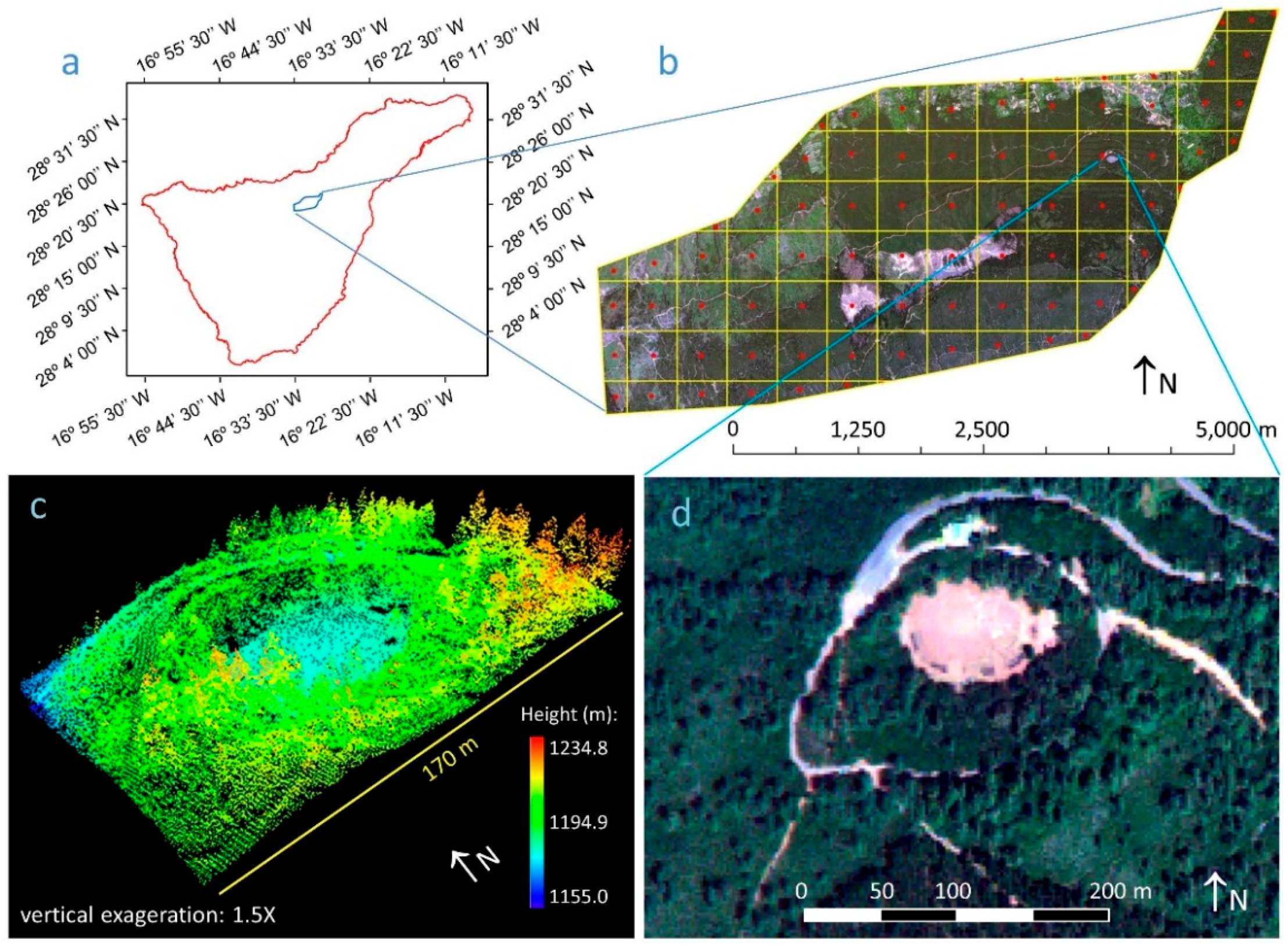
The study area (Figure 1), with coordinates 28°20′10′′N–16°29′36′′W and 28°22′11′′N–16°33′44′′W (WGS_1984_UTM_Zone_28N), is located on the north face of the Island of Tenerife (Canary Islands, Spain). The vegetation on Tenerife Island is a climatophilous one [55]. This means that vegetation is conditioned by the dominant climatic factors in the region. Additionally, there is a direct relation between the type of vegetation and the height at which it is found and, so, of the forest fuels present, as well. The prevailing trade winds’ regime blowing from NE transfer heavily humid air from the ocean to the north face of the island, where it is forced to ascend, due to the mountains, and forms clouds around a thermal inversion located on average between 800 and 1200 m above sea level (masl). Above this height, the air is drier, and the typical vegetation, mainly pine tree forests, is the same as that found on the south slope of the island at the same height.

The study area belongs to La Orotava municipality and it covers 15 km². La Orotava municipality stretches from sea level to the top of Teide volcano (the highest Spanish point, at 3718 m). In other words, it is the Spanish municipality with the highest variation in height. Regarding land cover, most of La Orotava is covered by natural areas (89%), of which approximately 30% correspond to forest areas. Showing an elevation range between 800 and 1650 masl, the study area is characterized by a highly rugged terrain and the presence of numerous ravines. It covers mostly forested areas, including 38% of the total forested area of La Orotava municipality and showing the highest vegetation diversity in the region. Vegetation is distributed within two altitudinal levels: Myrica-Erica evergreen forest (Myrico fayae-Ericion arboreae Oberd.) and laurel forest (Pruno hixae-Lauretalia novocanariensis Oberd. Ex Rivas-Martínez, Arnaiz, Barreno & Crespo) up to 1100 masl; altitudes above 1100 masl are dominated by formations of autochthonous Canary Pine (Pinus canariensis C.Sm. ex DC.), occasionally combined with stands of an introduced species, Monterey pine (Pinus radiata D. Don.).

3. Materials and Methods

3.1. LiDAR Data

Discrete, small-footprint and multiple-return LiDAR data were gathered by means of a Leica ALS60 sensor from July to August 2010. The sensor was mounted on a Cessna 421 Golden Eagle light aircraft, reaching a maximum flying height of 2000 m above the ground. This system received four returns per laser pulse and recorded return time and intensity (8-bit radiometric resolution). The field of vision varied between 35° and 45° with a 20% sidelap and a 1660-m full swath width. Point density by square meter averaged 2.43, showing a horizontal and vertical spatial accuracy of 60 and 20 cm, respectively. LiDAR information was provided by GRAFCAN (the company responsible for the cartography of the Canary Islands). The points provided were not classified.

A total number of 83 LiDAR scenes was used (Figure 1). Each scene was 500 × 500 m in size. The code set out by the American Society of Photogrammetry and Remote Sensing (ASPRS) was used to filter the point cloud, resulting in two point groups, (1) ground points and (2) non-ground points, shaping the vegetation.

Based on ground points, a Digital Elevation Model (DEM) with 2-m spatial resolution was derived. The DEM (Figure 2) represents the bare ground surface of the study area. The procedure used to derive the DEM is explained in detail in [56]. A Digital Surface Model (DSM) with the same spatial resolution was produced with the points corresponding to the first return. This layer represents the surface of the study area, but it also includes the top of the canopy in areas with vegetation. Next, the Canopy Height Model (CHM) was estimated as the subtraction of DSM and DEM. Thus, CHM represents the height of the canopy, estimated as the difference between the top canopy surface and the underlying ground topography [57] (Figure 2). Furthermore, 13 relative density bins of non-ground points by altitude range were calculated. Relative densities by range were estimated as the quotient between the number of non-ground points for each altitude range and the total number of non-ground points for such pixel. Eight 0.5-m altitude ranges (between 0 and 4 m), four 1.0-m ranges (from 4 to 8 m), plus one range for all points above 8 m were taken into consideration. These layers were produced with rapidlasso LAStools [58].

3.2. Spectral Data

A WV2 satellite image was used. WV2 is a Very High spatial Resolution (VHR) commercial sensor orbiting since 2009. This sensor captures eight multispectral bands (2-m spatial resolution) and a 0.5-m panchromatic band (

Table 1. WV2 spatial and spectral resolution (adapted from [59]).

Spectral Band	Centre Wavelength (nm)	Spectral Range (nm)	Spatial Resolution (m)
Panchromatic	632	450–800	0.5
Coastal	427	400–450	2
Blue	478	450–510	2
Green	546	510–580	2
Yellow	608	585–625	2
Red	659	630–690	2
Red Edge	724	705–745	2
NIR 1	831	770–895	2
NIR 2	908	860–1040	2

).

An image acquisition window was fixed over the time of duration of the field work. The WV2 image was captured on 23 June 2011. A product known as a standard “ortho-ready product” was purchased and distributed through radiometric correction, projecting over a fixed-height base plan that enabled its orthorectification. Top-of-atmosphere radiance was estimated using the method described by [59]. Next, atmospheric effects were corrected through the application of the FLAASH (Fast Line-of-Sight Atmospheric Analysis of Spectral Hypercubes) [60] algorithm. Lastly, the resulting image was orthorectified using the DEM obtained from the LiDAR data (2-m spatial resolution). We used ENVI 5.3 software for the WV2 image data preprocessing. The panchromatic band was not used for the purposes of this study.

3.3. Field Data

Field work was conducted between May and August 2011. A total 83 field plots were analyzed and randomly separated into two groups: 40 training field plots and 43 validation field plots. Plots were located in each LiDAR scene’s centroid, making up a square netting of plots occurring each 500 m (Figure 1). Since vegetation in this study area is strongly influenced by bioclimatic belts and they show a clear pattern from north to south, linked to differences in elevation (see the DEM in Figure 2), this systematic sampling design is representative of the vegetation of this region. Certain plots were moved in order to cover all fuel types.

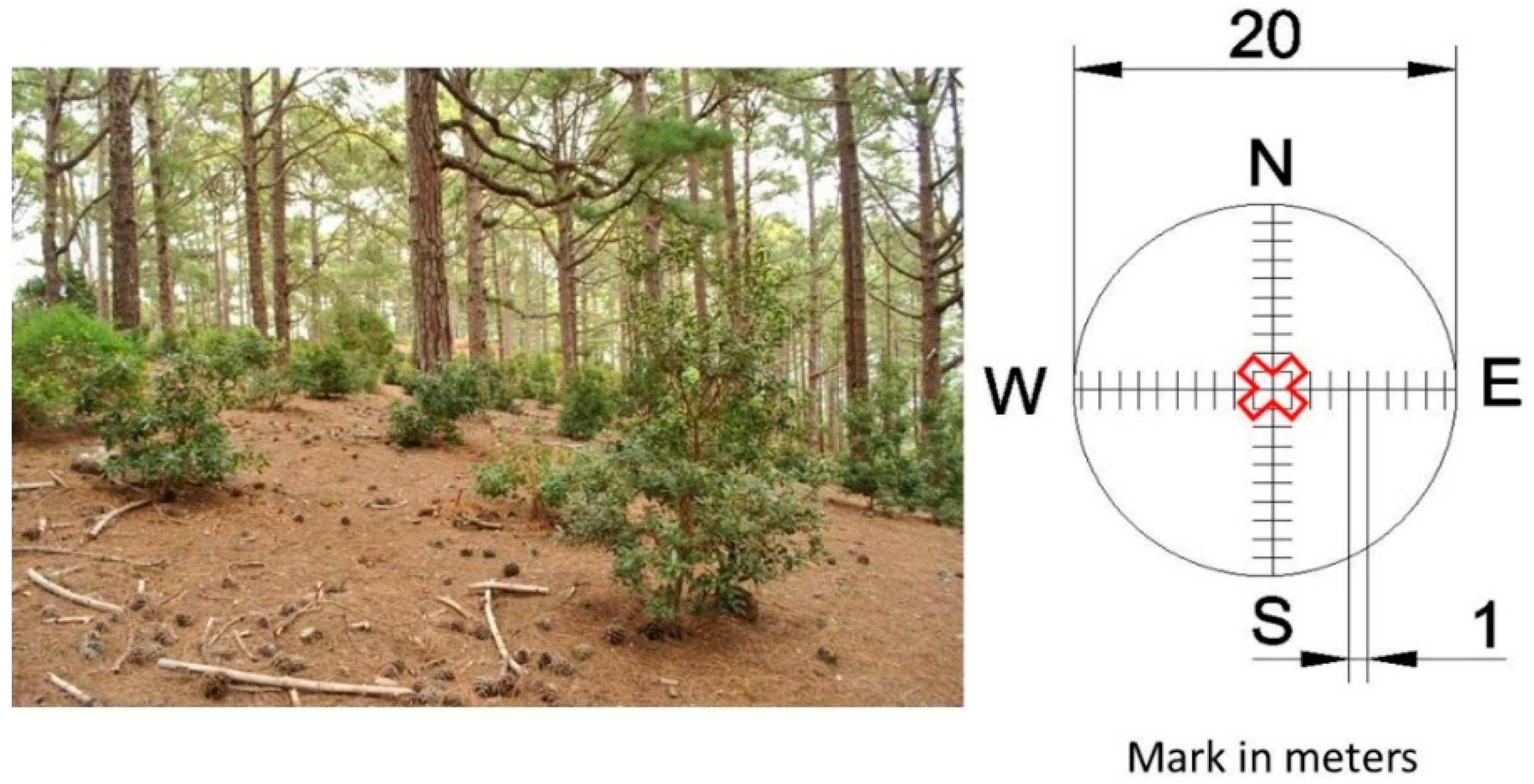
Circular plots with a 10-m radius and a 314-m² area were defined (Figure 3). A GeoExplorer GPS was used to measure the coordinates of the center of each plot, with a minimum 60 positions. A 2.5 m-high antenna was used to improve signal reception under the canopy cover. Within each plot, four 10-m transects were taken, according to the N, S, E and W directions. For each transect, measurements of each meter were taken, detailing: the presence/lack of vegetation cover, the species found, the vegetation height and the presence/lack of gaps between the understory and the canopy. Heights were measured using a Vertex Laser II digital hypsometer from Haglöf Sweden AB. Photographs of each transect were also taken as ancillary information for the identification of fuel types.

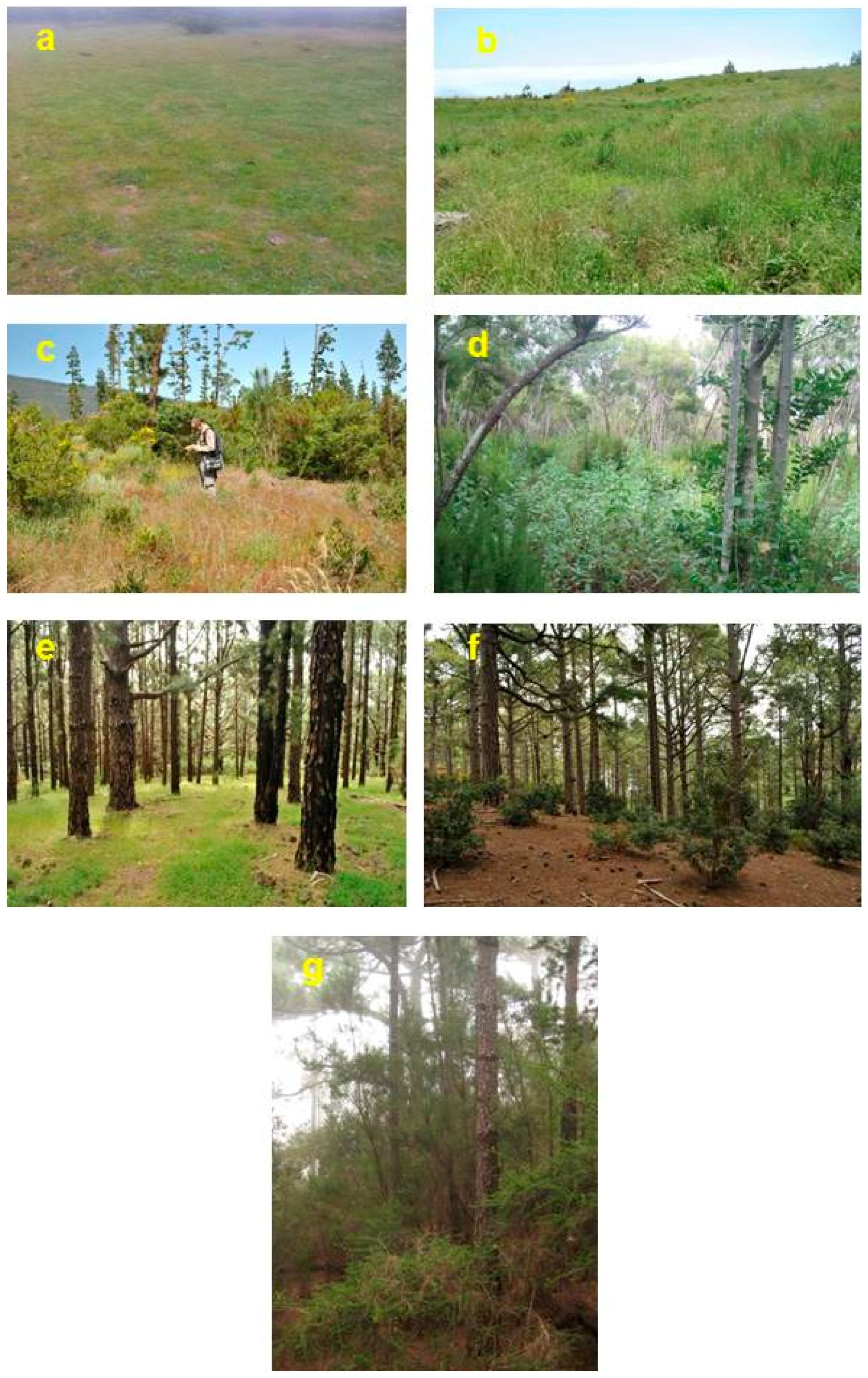
Using the information collected in the field, the fuel type corresponding to each plot was determined. The Prometheus Fuel Type (PFT) classification [14] was used as a model to identify the following fuel types according to horizontal and vertical vegetation structure:

• PFT1 (grass cover >50%): this category is primarily comprised by herbaceous vegetation and agricultural vegetation.
• PFT2 (shrub cover >60%, tree cover <50%): this category includes herbaceous vegetation and brushwood under 60 cm in height, as well as logging zones, where there are still remains of them.
• PFT3 (shrub cover >60%, tree cover <50%): areas showing medium-sized shrubs at or under 2 m in height.
• PFT4 (shrub cover >60%, tree cover <50%): areas showing big shrubs over 2 m tall and under the 4-m mark. This fuel type includes areas where young trees resulting from natural or artificial regeneration (by repopulation) occur.
• PFT5 (shrub cover <30%, tree cover >50%): forested areas dominated by tree cover with little or no understory.
• PFT6 (shrub cover >30%, tree cover >50%): forested areas showing either understory or logging residues where vertical distance between these and the trees’ first live branch is less than 0.5 m.
• PFT7 (shrub cover >30%, tree cover >50%): forested areas showing either understory or logging residues where vertical distance between these and the trees’ first live branch goes beyond 0.5 m, thus facilitating the vertical continuity of fires and favoring canopy fires.

For the study area, PFT1 was allocated in the areas where grasses start to take over bare grounds, agricultural vegetation and ravine beds with the occurrence of rupicolous vegetation comprised by species of the Aeonium spp., Aichryson spp. and Sonchus spp. genus. PFT2 was connected to areas of higher human impact, with an abundance of grass pastures dominated by buffelgrass (Cenchrus ciliaris L.), common thatching grass (Hyparrhenietum hirta (L.) Stapf), sage bush (Artemisio thusculae Cav.) and tree sorrel (Rumex lunaria L.). PFT3 corresponded to areas with a dominating presence of wild blackberry (Rubus inermis Pourr.) and bracken (Pteridium aquilinum (L.) Kuhn in Kersten) forming transitional communities towards more complex shrub formations. PFT4 was linked to brushwoods mainly formed by Montpellier cistus (Cistus monspeliensis L.), Canary Island flatpod (Adenocarpus foliolosus (Ait.) DC.) and bracken (Pteridium aquilinum (L.) Kuhn in Kersten), amongst other species. PFT5 matched the masses of Canary Pine (Pinus canariensis C.Sm. ex DC.) with no understory. Finally, PFT6 and PFT7 were found to be connected to Canary Pine forest formations showing a Myrica-Erica evergreen forest understory, laurel forests and natural regeneration of the pine forest itself. The difference between these two fuel types depended on whether or not there was vertical continuity from the understory to the tree layer. Figure 4 shows examples of PFT identified within the study area.

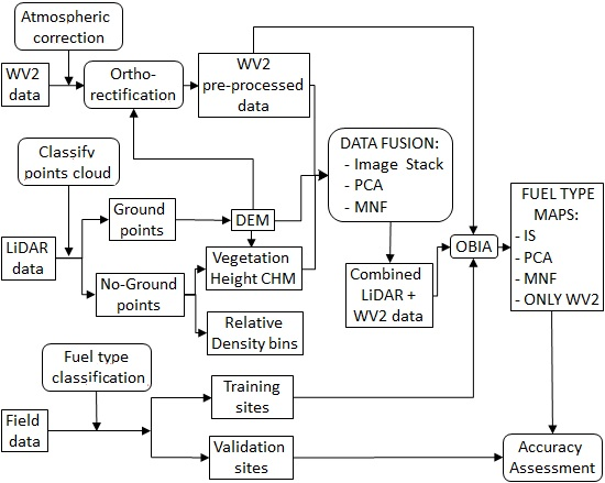
3.4. Image Data Fusion and GEOBIA Fuel Type Mapping

After data acquisition and pre-processing, three fusion methods were applied to combine the information from the LiDAR and WV2 imagery. The following fusion methods were used: IS, PCA and MNF. Then, the created image-fusion datasets, plus the WV2 image alone, were incorporated into four independent GEOBIAs to map the PFTs of the study area. Field work data were used for training the GEOBIA classifications and assessing the accuracies of the obtained fuel type maps. Field plots used for training were not used for validation. The classification of the field plots into those used for training and those used for validation was done randomly. 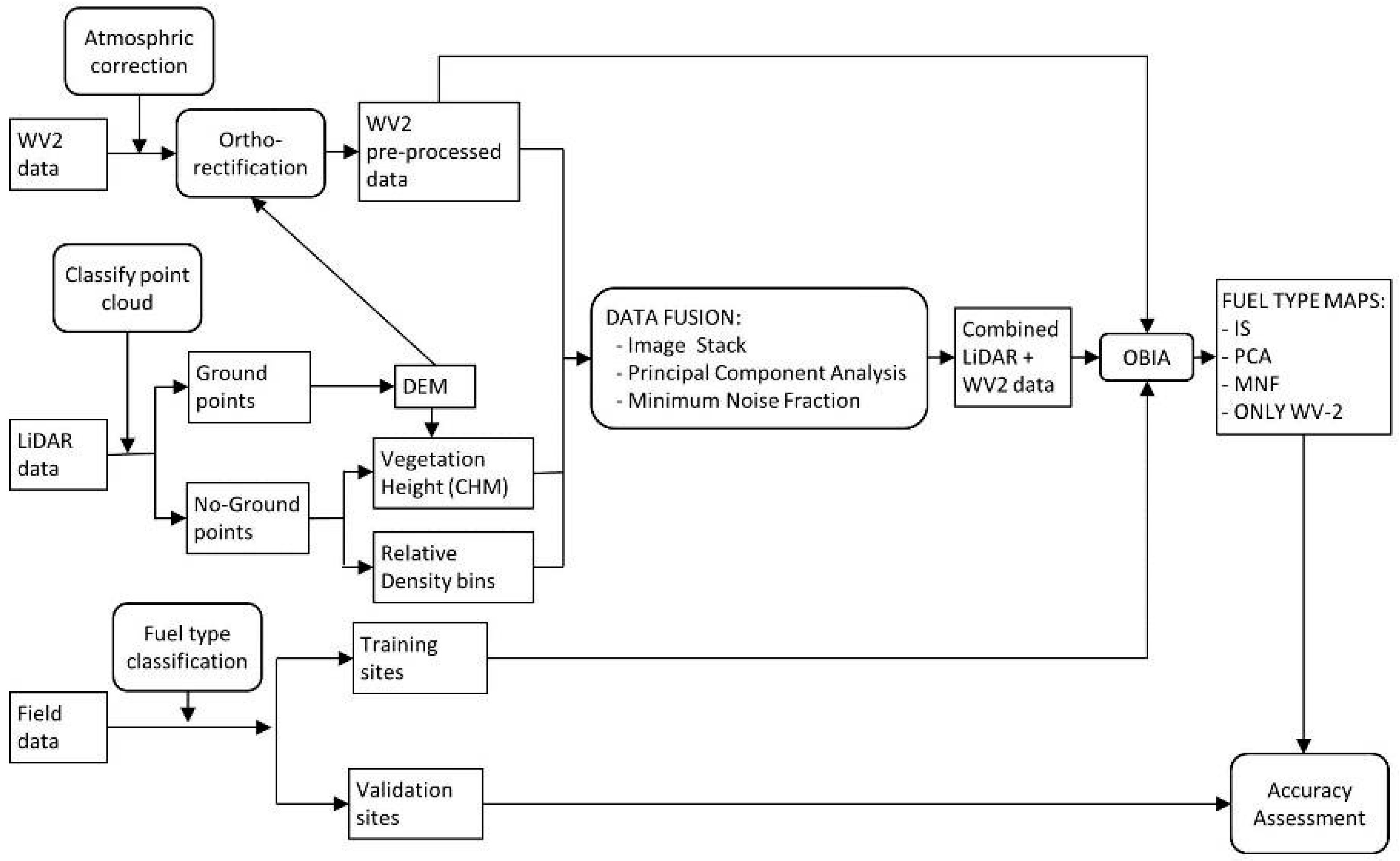Figure 5 displays the workflow used in the completion of this research work.

We used the software ENVI (Version 5.3) for image-fusion. An image dataset showing 22 bands and a spatial resolution of 2 m was produced for the IS fusion. Bands resulting from LiDAR information were directly merged with the pre-processed bands from the WV2 sensor. This way, the new image comprised 8 multispectral bands derived from the WV2 image and 14 bands obtained from the LiDAR data (13 for relative density by altitude range bins and the CHM).

The PCA method makes it possible to decrease the number of bands in the IS image dataset, in exchange for a small loss of information [61]. Statistics show that PCA will seek to accurately represent, whenever possible, the original information through a lesser number of bands, built as linear combinations of the original [62]. This allows the new bands to explain as much total variability as possible, where there is no correlation. The fused PCA image was comprised of the first 5 PCA bands, which explained 99.47% of the total variability of the IS image dataset.

The MNF method also attempted to reduce the number of bands in the IS image dataset by transforming its original bands. In this case, fused bands were estimated as the linear combinations maximizing the signal-to-noise ratio, thus minimizing existing noise [63]. For the MNF image-fusion, the first eight MNF bands were selected. These explained 99.3% of the variance in the IS image dataset.

Three fuel type maps were independently obtained from the three-image dataset created in the data fusion processes (IC, PCA and MNF). A further fourth fuel map was produced from the WV2 image in order to enable the comparison of results found against the classifications obtained from non-merged information.

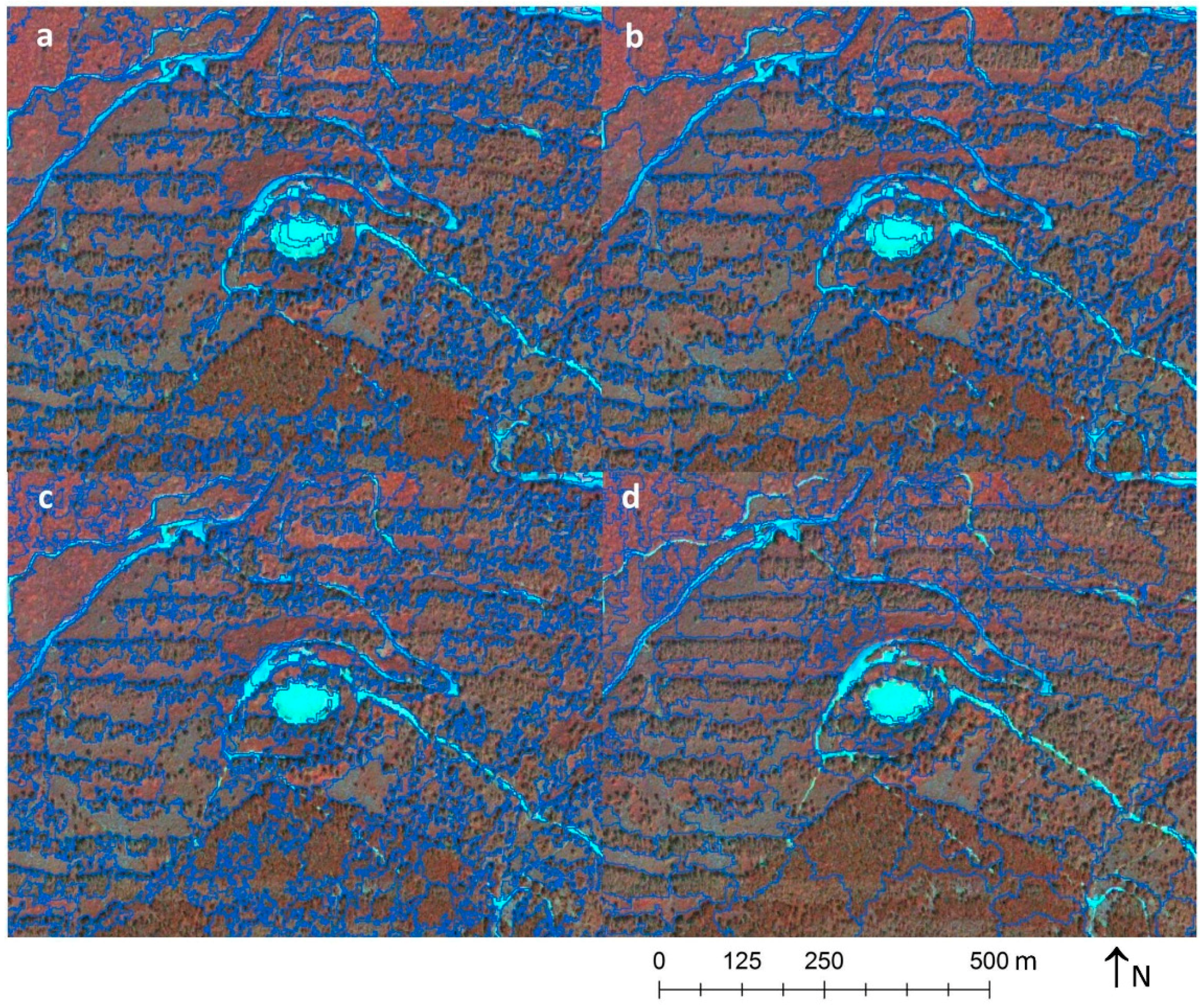
All classifications were conducted with GEOBIA, using Definiens 8.64 software. First, the image was divided into objects. This process started with one-pixel objects and gradually moved on to their attachment to adjacent objects [64]. Object internal heterogeneity was estimated by allocating weights equivalent to 0.8 for the color parameter and 0.2 for the shape parameter (0.3 and 0.7 for smoothness and compactness, respectively). The most suitable scale parameter was assessed through trial and error testing conducted until segmentation according to the features of each fuel type was achieved. Scale parameter values of 45, 45, 90 and 100 were set up for the IS, MNF, WV2-alone and PCA datasets, respectively. Image segmentation of the four datasets is shown in Figure 6. Segmentation included a thematic layer demarcating the testing plots so as to ensure their observance.

The next step was to classify the fuel types. Seven thematic classes were defined, in accordance with the fuel types included in the Prometheus classification. The Nearest Neighbor (NN) classifier implemented on eCognition software was used during the allocation phase. The GEOBIA NN classifier performs a supervised classification. It applies the same strategy as the pixel-based NN classifier. The only difference is that it uses objects instead of pixels; this means that object-based features, such as those related to internal variability within the object, can be considered for the classification. First, the classifier was trained with the 40 field plots set aside for this task. The same field plots were used for the four classifications. Then, the classifier assigned each object in the image to a Prometheus fuel type, based on its minimum distance to the training samples. Distances were estimated taking into consideration the following objects-based features: average values in all bands, standard deviation in all bands, brightness and maximum difference. The same features were used for the four classifications. Lastly, adjacent objects allocated to the same fuel type were merged in order to homogenize the final map.

3.5. Accuracy Assessment

Accuracy of the resulting maps was assessed through overall agreement analyses and the estimation of overall quantity and allocation disagreements, as suggested by [65,66,67]. The field plots reserved for accuracy assessment were used for this part of the analysis. Quantity disagreement refers to the differences between the obtained map and the reference data (i.e., field data) in the surface covered by the fuel types. Allocation disagreement is related to the differences between the obtained map and the reference data in the spatial distribution of fuel types. Overall disagreement is the sum of overall quantity disagreement and overall allocation disagreement; and is complementary to the overall agreement. Map accuracy was also analyzed per category. Thus, relative allocation disagreement and relative quantity disagreement were estimated for each fuel type. These per-category disagreement measures are similar to those used to assess the maps’ global accuracies. The only difference lies in the fact that such by-category estimations were related (i.e., they were assessed considering the total area covered by each category in the map), so as to enable comparison of results across categories. See [67] for more details.

From the 83 field plots, 43 were set aside and used for disagreement estimation tasks. Each plot was linked to a 10 × 10 pixel window. Fuel types are complex elements, and so, they cannot be assessed for very small areas, or individual pixels. The vertical and horizontal structure of vegetation needs to be taken into consideration. For that reason, fuel types were estimated on field plots larger than the pixel size. Although the field plots size was slightly smaller than 10 × 10 pixels (314 m² instead of 400 m²), we deemed it appropriate to use such a window size, since boundaries between fuel types are fuzzy, meaning that the inclusion of a small buffer around each field plot would not affect the results of the accuracy assessment. Fuel types identified in the field for these plots were compared to the results corresponding to the four maps obtained.

Finally, we used McNemar’s test [68,69] to assess whether the differences observed in overall accuracy were significant. This statistical test was chosen because it is suitable for comparing thematic maps when the same set of field sites is used for the accuracy assessment. We used the following test equation:

$$X^2=\frac{{\left(\left|f_{CI}-f_{IC}\right|-1\right)}^2}{f_{CI}+f_{IC}}$$

where:

• f_CI is the number of sites correctly assigned in Map 1 and incorrectly assigned in Map 2.
• f_IC is the number of sites incorrectly assigned in Map 1 and correctly assigned in Map 2.

The derived values were compared against the chi-squared distribution and a statistical significant value of 0.05.

4. Results

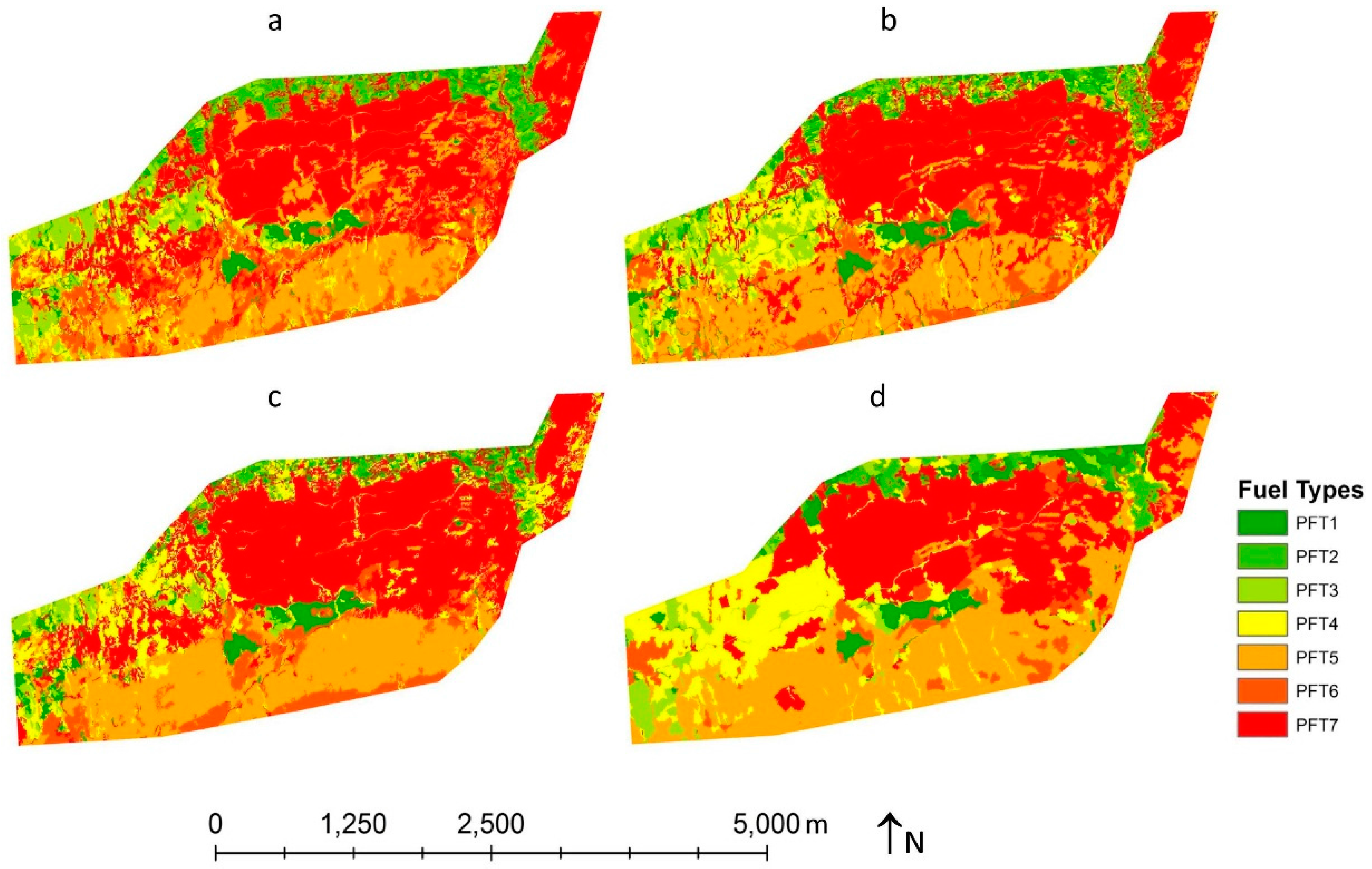
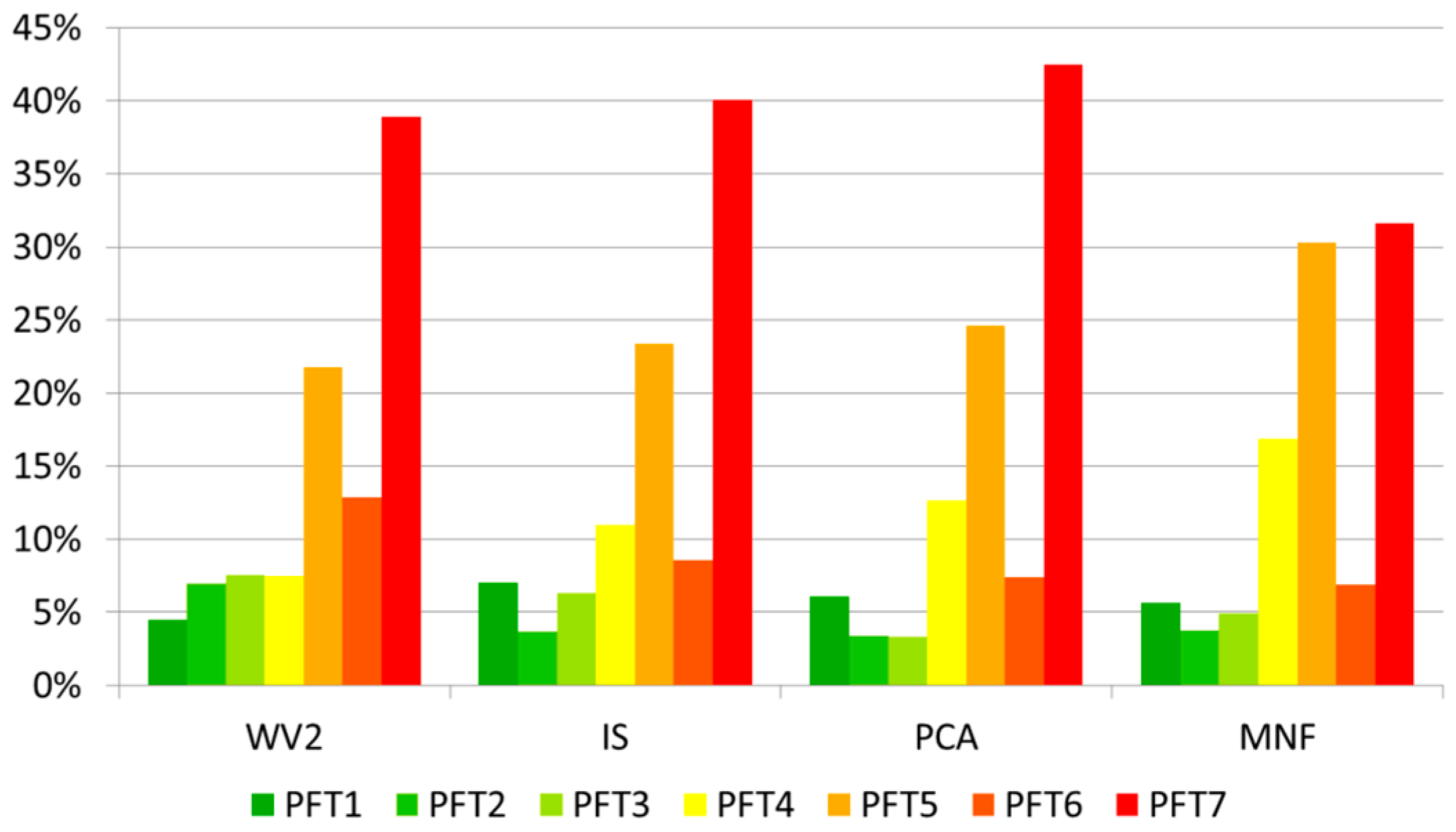
Four fuel type maps were created, three resulting from image-fusion datasets (IS, PCA and MNF) and another one from the WV2 image alone (Figure 7). Figure 8 shows the relative surface covered by each fuel type in all four maps.

Results are similar across all classifications. PFT7 is the fuel type covering a greater surface, taking up a relative surface of over 30% in all cases. This fuel type corresponds to the greenwood and Myrica-Erica evergreen forest bordering agricultural vegetation areas found in the northeastern segment of the study area and to canary pine forests in the central segment. Higher altitude areas, located in the southern segment of the study area, are primarily covered in canary pine forests with no understory, largely allocated to PFT5. This fuel type takes up from 22% to 30% of the field of study, according to the various classifications. The remaining fuel types are less abundant and more or less disaggregated over the study area. Visually, the most remarkable differences can be identified in the map resulting from MNF image-fusion, which shows a more homogeneous appearance, with larger polygons. Thus, the average size of polygons in the map resulting from MNF image-fusion virtually doubles that of the rest of the maps. Furthermore, surfaces covered by PFT4 and PFT5 in the MNF-derived map are larger than those in the other maps, whereas the surface allocated to PFT7 is noticeably smaller.

Global agreement for maps obtained varies from 76.23% to 85.43% (

Table 2. Overall and per-fuel type measures of accuracy (overall and relative quantity disagreement; overall and relative allocation disagreement) for the four fuel type maps (values in %).

	WV2		IS		PCA		MNF
	Quantity	Allocation	Quantity	Allocation	Quantity	Allocation	Quantity	Allocation
PFT1	0.61	1.50	0.08	1.95	2.03	2.45	0.11	0.00
PFT2	1.86	2.61	0.92	5.28	3.25	1.11	0.47	0.00
PFT3	5.92	0.00	2.03	3.39	0.64	2.06	3.11	0.00
PFT4	3.59	1.11	0.14	2.45	1.64	6.51	1.70	1.06
PFT5	1.78	12.18	3.28	1.56	2.28	0.00	1.75	6.62
PFT6	5.81	2.11	2.67	0.44	2.98	0.00	0.78	5.56
PFT7	3.89	4.56	1.50	5.78	0.36	4.84	1.81	6.17
Overall	11.73	12.04	5.31	10.42	6.59	8.48	4.87	9.71

). The lowest global agreement obtained corresponded to the map produced from the WV2 image alone, totaling 76.23%. McNemar’s tests confirmed that differences found in global agreement for the WV2-derived map and the ones obtained from the three image-fusion databases were significant in all cases (p-value of 0.05). Maps produced by means of image-fusion showed a global agreement ranging from 84.27% to 85.43%. Differences in global agreement across the three tested fusion methods were not significant in any case, according to McNemar’s tests. Allocation and quantity components of error were estimated so as to enable the analysis of any disagreements found (Table 2). The overall quantity disagreement tells us the extent to which the proportions of fuel types found for each map differ from the real proportion of fuel types (based on field assessment); and overall allocation disagreement shows the degree to which geographical distribution of fuel types by maps is different from the actual location of fuel types in the study area (based on field measurements). Maps produced from MNF and IS datasets showed less quantity disagreement than allocation disagreement, with almost double error due to the wrong allocation of fuel types. This uneven distribution of error components was not seen in maps produced from PCA and WV2.

Besides global disagreement measures, quantity and allocation disagreement for each fuel type were estimated across all four maps (Table 2). Rather than absolute measures, we used their relative versions in order to be able to compare fuel types [67]. PFT1 was the fuel type showing fewer disagreements, with values under 2.5% in all cases. This fuel type is basically comprised of herbaceous vegetation and agricultural vegetation, which was identified accurately both in the WV2 image alone and in the three LiDAR-fused datasets. At the other end of the spectrum, the fuel type showing a higher disagreement rate was PFT7, corresponding to dense canary pine formations and Myrica-Erica evergreen understory. Disagreement in PFT7 identification occurred across all maps, both in the WV2 image alone and in the three fusion datasets. Regarding classification on the WV2 image, optical information did not lead to obtaining information on vegetation occurring under the tree cover. In terms of classifications on image-fusion, this can probably be explained by the low point density of LiDAR data, which proved insufficient in certain cases. In areas of dense canopy cover, the number of returns originated in the ground and lower strata noticeably decreased, making it difficult to tell these different fuel types apart.

By analyzing disagreement by categories, a more detailed study of the selective goodness-of-fit of each method for each fuel type was possible. When comparing the results of the WV2 classification against the WV2 and LiDAR fusions, the biggest differences in disagreement were found in Fuel Types 5 to 7. Differences were not as marked in remaining fuel types. Indeed, they were non-existent in certain cases. This way, PFT1 and PFT2 showed similar or lower disagreement rates on the map derived from the WV2 image than on those from IS and PCA datasets. Based on this finding, optical information gathered by the WV2 was enough to identify those fuel types without canopy cover. Contextual information, entered in the system through GEOBIA, made this possible. In order to identify other fuel types, on the other hand, the lack of information on the vertical distribution of the vegetation proved particularly limiting. Another noteworthy fact is that agreement reached by the classification on the MNF dataset was biased towards herbaceous or shrub fuel types. For the MNF fusion, LiDAR information provided the identification for fuel types without tree cover, but it barely showed any improvements on the WV2-based classification concerning the rest of the fuel types. Thus, when comparing the three fusions, the classification on the MNF image-fusion resulted in the lowest disagreement rates across all fuel types without tree cover (PFT 1 to 4) and the highest disagreement rates for fuel types including tree cover (PFT 5 to 7). Given that all three fusion methods are initially based on the same information, this difference can only be due to the merging process itself. Nonetheless, the knowledge of the disagreement distribution in the produced maps is vital: (1) when choosing the most suitable mapping method, according to the specific objectives of each project; and (2) towards learning about the disagreements that can be expected with each method.

5. Discussion

The results of this study corroborate the ability of GEOBIA to differentiate complex elements, such as fuel types, on high spectral heterogeneity data, such as VHR imagery. Introducing context features into the analysis aided in the identification of PFT. Image segmentation further allowed converting the original working scale, imposed by the image’s spatial resolution, into a working scale suited for the purposes of this research (i.e., fuel type identification). Previous similar researches conducted on different types of images and fields of study have nonetheless led to much the same conclusions [19,25,54].

Global agreement values across all maps improved by at least 10% once information on the vertical distribution of vegetation was incorporated by means of fusion with LiDAR data. It should be noted that this significant improvement in the maps’ accuracy was achieved through the use of medium-to-low density LiDAR data (2.43 points/m²) gathered in a study area of highly complex orography. Previous studies had shown that the combined use of optical and LiDAR information allows for improved fuel type identification [50,51,52]. Generally speaking, global agreement values were similar and, on occasion, even higher than those reached in this study. Nonetheless, for the most part, these were obtained with better-quality information (i.e., higher spatial and spectral resolution of optical images and higher point density in LiDAR data). In the study presented by [50], for example, a support vector machine classification combining imagery from Airborne Thematic Mapper (10 spectral bands with 2-m spatial resolution) and LiDAR imagery produced fuel maps showing 89% accuracy when using fusing. Similar improvement in results were found by other authors when classifying fuel types on image-fused QuickBird and LiDAR datasets rather than against the QuickBird image alone [51]. The abovementioned researchers obtained a 90% global agreement in the classification of an MNF image-fusion; an edge of almost 5% as compared to this research’s results. However, as pointed out by [52], such positive results might be explained by the characteristics of the study area, an area of no orographic complexity and the fewer fuel types occurring within it. For an orographically-complex region, 76% global agreement has been obtained by combining four-band multispectral imagery from the National Agricultural Imagery Program with low point density LiDAR data [52].

The developed methodology could be applied to larger areas on the north face of Tenerife Island and with similar elevation, where vegetation is strongly influenced by the climatic conditions imposed by elevation and the trade winds. This situation actually affects the entire forest surface on the island of Tenerife, as well as the remaining occidental islands of the Canary archipelago (Gran Canaria, La Palma, La Gomera and El Hierro). In other words, this methodology could potentially be used to generate fuel type maps of the forested areas of all of these islands. For those areas not influenced by trade winds, vegetation is very different due to the lack of humidity. For those areas, this methodology might not be suitable. Variability in vegetation may become too large, and the systematic sampling design for field plots may not be representative.

The results of this study could become a very important tool for fire fighters and other forest managers in the region. Accurate and up-to-date fuel type maps are a very valuable source of information for the forest fire prevention planning (e.g., preventive silvicultural treatments), as well as for the firefighting implementation systems. For all of the above-mentioned islands, fuel maps have not been updated in more than 10 years. Moreover, these maps do not show the spatial resolution obtained through the fusion of WV-2 and LiDAR, nor do they cover the whole area that could be affected by the great forest fires that ravage our islands, such as the concurrent ones in the summer of 2007 in Tenerife and Gran Canaria, which burnt 16,820 and 18,762 ha, respectively.

No evidence has been found pointing at a fusion method prevailing over the others in terms of global agreement reached. We can therefore assume that the differences found are simply due to chance. Consequently, choosing the best fusion method for any given research may essentially depend on the specific purposes of each project, as well as on the means available to it (i.e., processing time and software required for each fusion technique). However, when allocation and quantity components of error were estimated, the differences were most evident. Maps created from MNF and IS (i.e., with a lower overall quantity disagreement) would be especially suitable for studies aiming to analyze the evolution of fuels over time, for instance. The PCA fusion method would be recommended when the exact spatial location of the various fuel types is needed. This would be the case of any study targeting decision-making on early detection and active fire control, in order to determine the appropriate location for watchtowers, for example. In line with factors discussed in previous sections, LiDAR fusion would be recommended in all cases, since maps produced by the WV2 image alone cause a higher disagreement rate both in quantity and allocation.

6. Conclusions

In the course of this study, we have assessed the viability of combining GEOBIA and VHR multispectral imagery (WV2) and discrete low-density LiDAR data aiming to obtain fuel type maps in the Canary Islands. To that end, four independent GEOBIAs were produced by means of three fused images (IS, PCA and MNF) and one non-fused WV2 image. Global agreement of the resulting maps has exceeded 75% in all cases. These results corroborate the ability of GEOBIA to differentiate complex elements, such as fuel types, on high spectral heterogeneity imagery.

Maps obtained through VW2 and LiDAR data fusion reached a significantly higher global agreement versus those generated by the WV2 image alone. By integrating LiDAR information with the GEOBIAs, global agreement improvements by over 10% were attained in all cases. Such results are especially relevant when considering the nature of the LiDAR information used. In contrast with other studies conducted with full-wave, higher point density LiDAR information, this research has been based on low point density LiDAR data. This information was used due to it being a database accessible and free of charge throughout the Canarian territory. Therefore, we did not incur any costs to use it.

All three fusion methods used in this study (IS, PCA and MNF) provide similar results, and we were unable to identify major differences in global agreement values. Any of the above can be used with an expected disagreement rate of approximately 15%. Concerning the choice of any of them for a specific project, the particular purposes of each specific project should be taken into consideration. For that purpose, we suggest a detailed assessment of per-fuel type quantity and allocation disagreement.

One of the main limiting factors facing the production of fuel maps in the Canary Islands is the presence of areas of great orographic complexity paired with dense canopy covers of over 30 m in height. Such characteristics decrease the efficacy of LiDAR data to represent the vertical structure of vegetation, especially when working with low point density data. What is more, the occurrence of ravines and highly rugged terrain causes shading effects, which are also difficult to correct in the optical imagery, besides impacting image geometric correction. All of the above negatively affect fuel type identification. The findings of this research work show that it is possible to minimize such limitations through the combined use of GEOBIA and WV2 and LiDAR fusion. This methodology could potentially be used to generate fuel type maps of the forested areas of all of the occidental islands of the Canary Archipelago.