An Inter-Comparison Study of Multi- and DBS Lidar Measurements in Complex Terrain

Abstract

Wind measurements using classical profiling lidars suffer from systematic measurement errors in complex terrain. Moreover, their ability to measure turbulence quantities is unsatisfactory for wind-energy applications. This paper presents results from a measurement campaign during which multiple WindScanners were focused on one point next to a reference mast in complex terrain. This multi-lidar (ML) technique is also compared to a profiling lidar using the Doppler beam swinging (DBS) method. First- and second-order statistics of the radial wind velocities from the individual instruments and the horizontal wind components of several ML combinations are analysed in comparison to sonic anemometry and DBS measurements. The results for the wind speed show significantly reduced scatter and directional error for the ML method in comparison to the DBS lidar. The analysis of the second-order statistics also reveals a significantly better correlation for the ML technique than for the DBS lidar, when compared to the sonic. However, the probe volume averaging of the lidars leads to an attenuation of the turbulence at high wave numbers. Also the configuration (i.e., angles) of the WindScanners in the ML method seems to be more important for turbulence measurements. In summary, the results clearly show the advantages of the ML technique in complex terrain and indicate that it has the potential to achieve significantly higher accuracy in measuring turbulence quantities for wind-energy applications than classical profiling lidars.

1. Introduction

Over recent years, lidar (light detection and ranging) technology has quickly penetrated wind-energy applications. Especially in resource assessment, Doppler lidars are now widely used for wind measurements to predict the annual energy production of windfarms. In flat and homogeneous terrain, classical profiling lidars using the Doppler beam swinging (DBS) or velocity azimuth display (VAD) techniques achieve high accuracy [1]. Therefore, in recent years, their use has been adopted into national and international standards and guidelines [2,3].

The application of Doppler lidars in complex terrain, however, remains difficult and is often associated with systematic errors in mean wind-speed estimations [4,5]. If the flow is complex, the homogeneity assumption underlying the DBS and VAD techniques is often violated. First comparison studies have shown promising results in the capabilities of flow models in correcting this complex terrain error at individual sites [4,6]. However, they also indicated a high sensitivity to model parameterisations [6] and remain limited to moderately complex terrain. Moreover, the application of corrections leads to an increased uncertainty.

Another disadvantage of profiling lidars compared to mast-based measurements is that the estimation of turbulence characteristics, which are, e.g., relevant for wind-turbine loads, is not possible with the desired accuracy [7,8,9]. Most prominently, the estimation of the variance of the wind-vector components and the respective spectra suffer from systematic errors due to the effects of cross-contamination and volume averaging [9,10]. Newman and co-workers showed that some of the cross-contamination effect can be mitigated by applying a correction based on the measurement of the vertical variance [11]. However, their experimental results indicated that even after the application of the correction, a large deviation between lidar and mast-based measurements can remain. In general, a turbulence correction is difficult since it depends not just on lidar technology and measurement configuration but also the three-dimensional structure of the turbulence itself and, as a consequence, on atmospheric conditions [8,9]. New scanning strategies thus need to be developed. A promising example is the six-beam method [12,13], where turbulence parameters are directly derived from the radial velocity variances. Although the first encouraging experimental results have been reported in [12], other experiments indicated mixed results [11]. In complex terrain, the six-beam method might also be affected by an inhomogeneous turbulence field.

Probably the most intuitive solution to reduce the potential errors in lidar measurements is to set up multiple lidars such that the various lidar beams intersect at a single point from different directions (muti-lidar technique or ML). This strongly reduces the need for flow homogeneity in lidar measurements. Moreover, intersecting lidar beams probably offer the best approach to derive highly resolved time series of the three-dimensional wind-vector and turbulence statistics [14].

In flat and homogeneous terrain, first experimental results intersecting three lidar beams next to a sonic anemometer showed encouraging results for mean wind speeds [15,16,17] and turbulence statistics [14,16]. Mann and co-authors showed good agreement between second-order turbulence statistics of the radial wind velocities from multiple lidar systems and a sonic anemometer measurement [14] which was corrected using the spectral tensor model of [18]. Fuertes and co-authors achieved good agreement in second-order turbulence statistics between three intersecting lidars and a sonic anemometer to which they applied a simpler, pseudo-spatial filtering approach [16]. However, both studies were performed under idealised conditions in flat and homogeneous terrain and only report on very limited sample sizes. Newman and co-workers have also used three lidar beams intersected in a single point to derive turbulence statistics [19], but no adequate reference was available to assess the accuracy of their measurements.

This paper presents measurements performed during the Kassel 2014 Experiment. The aim of the Kassel 2014 Experiment was to experimentally explore and demonstrate the advantages of ML measurements under conditions which are realistic for wind-energy applications in complex terrain. The experiment also served as a test bed for the complex terrain experiments in the New European Wind Atlas which will heavily rely on ML measurements [20]. Here, we present measurements and comparisons of four long-range WindScanners, which intersected at one point, a DBS lidar, and a sonic anemometer at a reference mast at a complex forested site. An analysis of the radial velocity statistics is used to examine the measurement accuracy of the individual instruments as well as the accuracy of the setup process. It is also used to provide insight into the path-averaging effect on turbulence measurements with the WindScanners. An analysis of the first- and second-order statistics of the horizontal wind speed contrasts error sources for the different lidar techniques.

The ML-DBS-mast inter-comparison is especially valuable to analyse and quantify the benefits of the ML technique over the standard DBS lidar and experimentally compare their measurement behaviour in complex terrain. The WindScanners were located at distances ranging from directly next to the mast to 3740 m from the reference mast; they reflect a measurement scenario which is “realistic” in windfarm development scenarios in complex terrain.

2. Materials and Methods

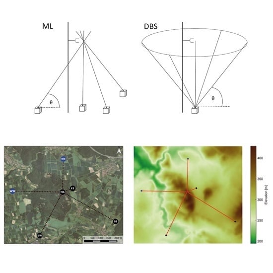
2.1. Wind Vector Reconstruction and Scanning Strategies

Doppler lidars provide an estimate of reflectivity-weighted, radial velocities of aerosol particles. This velocity was applied as a good approximation for the radial wind velocity. In the context of wind profilers, the difference between Doppler velocity and real-wind velocity has been addressed by [21]. For Doppler lidars, the assumption seems justified as most of the backscattering for optical wavelengths is from particles which are small enough to be advected with the wind (e.g., [22]). Moreover, a homogeneous aerosol concentration within the probe volume needs to be assumed at this point. The measured radial velocity $\left(v_{r i}\right)$ is thus a projection of the three-dimensional wind vector ($v$) onto the lidar beam

$$v_{r i}= v_{\mathit{i}}·{\mathit{n}}_{\mathit{i}},$$

(1)

where ${\mathit{n}}_{\mathit{i}}$ is the unit vector in the direction of the lidar beam and $i$ denotes the individual beam and its location. In meteorological applications, it is convenient to write this equation as:

$$v_{r i}= u_i\cos ({\mathsf{\theta }}_i)\cos \left({\mathsf{\varphi }}_i\right)+v_i\cos \left({\mathsf{\theta }}_i\right)\sin \left({\mathsf{\varphi }}_i\right)+w_i\sin \left({\mathsf{\theta }}_i\right),$$

(2)

where $u$ is directed into the mean wind direction during the averaging interval, $v$ is perpendicular to $u$ in the horizontal and $w$ is the vertical component of the wind vector. The projection onto the radial is defined by the elevation angle $\mathsf{\theta }$ in addition to the angle between the mean wind direction and the beam $\mathsf{\varphi }$. The azimuth angle ($\mathsf{\psi })$ or beam-pointing angle is often used instead of $\mathsf{\varphi }$ in the literature to define (2). However, in this paper, the use of $\mathsf{\varphi }$ makes the notation in the later chapters more consistent.

Assuming homogeneous flow (i.e., $v_i=v$) between the measurement locations or—as is the case for ML configurations—the intersection of the beams in a single location, multiple measurements can be combined to derive $v$ using matrix inversion

$$v= {\mathit{M}}^{-\mathbf{1}}·{\mathit{v}}_{\mathit{r}},$$

(3)

where $\mathit{M}=\left\{{\mathit{n}}_{\mathbf{1}},{\mathit{n}}_{\mathbf{2}},\dots \right\}$. For a reconstruction of all components of $v$, at least three beams need to be combined.

The horizontal wind speed ($V_h)$ is then defined as:

$$V_h= \sqrt{u^2+v^2}.$$

(4)

Classical profiling wind lidars usually rely on a scanning strategy, which employs a conical scan above the instrument and measures $v_{r i}$ at a fixed height and at different azimuth angles. The wind profiler lidar (manufacturer Leosphere, type Windcube v2), which is used as a reference instrument in this study, scans in DBS mode and uses four beams (with $\mathsf{\theta }=62°$), which are arranged in two perpendicular planes (Figure 1). An additional vertical beam is used to measure $w$ directly. The resulting separation between two opposing beams in this setup is roughly equal to the measurement height.

Especially in complex terrain, the assumption of homogeneous flow across the different beams of a profiling lidar is often violated; significant, direction-dependent errors in the estimation of the mean can be introduced [4,5]. The main reason for the observed errors is thought to be the difference in $\overline{w}$ (the overbar denotes the mean) across the different beam locations [4,5]. Differences in the other components will of course also introduce an error. For the site of the current experiment, a deviation to mast-bound cup anemometer measurements of approx. −4% to +2% in $\overline{V_h}$ has previously been reported [6]. Also the scatter in the inter-comparison was higher than in comparable experiments in flat and homogeneous terrain [1].

In contrast to profiling lidars, the ML-technique uses a combination of multiple lidars, which are located around the measurement location and focus their laser beams to intersect in a single location (Figure 1). Since multiple independent measurements of the radial velocity are made at the point of interest, the assumption of horizontal homogeneity of the mean flow among the different beam locations is not needed. The effect of a potential inhomogeneity within the probe volume of the ML measurement is expected to be much smaller and the beam separation problem inherent in a profiling lidar measurement is potentially overcome.

2.2. Second-Order Statistics of $v_r$

One of the characteristics of wind-speed measurements from Doppler lidars is that, due to the measurement principle, $v_r$ is retrieved from a measurement within a probe volume. The width of the laser beam is usually negligible compared to the length of the probe volume along the path. The effect of the measurement volume on $v_{r lidar}$ can thus be simplified to line averaging along the direction of the lidar beam. This can be expressed as

$$v_{r lidar}= {\int }_{-\infty }^{\infty }\phi \left(s\right)\mathit{n}·V\left(r+\mathit{n}\mathrm{s}\right)ds,$$

(5)

where $\phi \left(s\right)$ is the weighting function along the probe volume, $r$ is the centre of the probe volume and $V$ is the three-dimensional velocity field. Depending on the signal processing and shape of the emitted laser pulse, $\phi \left(s\right)$ will vary and different forms have been suggested (e.g., [23,24]). Here we follow the concept that the weighting function can be estimated from a convolution of the form of the laser pulse ${\phi }_p\left(s\right)$ and the gate-weighting function ${\phi }_g\left(s\right)$, which results from the size and shape of the sampling gate—i.e., the internal signal processing [25]. Since the effects of line averaging depend on the scale of the turbulent eddies, it is convenient to express the problem in Fourier space. The Fourier transform of (5) can be written as [14,26]:

$${\widehat{v}}_{r lidar}\left(\mathit{k}\right)= \widehat{\phi }\left(\mathit{k}·\mathit{n}\right)\mathit{n}·\widehat{V}\left(\mathit{k}\right),$$

(6)

where $\mathit{k}$ is the wave vector $\left(k_1,k_2,k_3\right)$ and ^ denotes the Fourier transform. For the WLS 200s (a scanning lidar manufactured by Leosphere) used in this study, both weighting functions can be approximated by a Gaussian function [27]. $\widehat{\phi }\left(\mathit{k}\right)$ can thus be approximated by

$$\widehat{\phi }\left(\mathit{k}\right)={\widehat{\phi }}_p\left(\mathit{k}\right){\widehat{\phi }}_g\left(\mathit{k}\right)=e^{-{\mathit{k}}^2{\sigma }_p^2/2}{e}^{-{\mathit{k}}^2{\sigma }_g^2/2},$$

(7)

where ${\sigma }_p$ is the standard deviation of ${\phi }_p\left(s\right)$ and ${\sigma }_g$ is the standard deviation of ${\phi }_g\left(s\right)$.

In practice, pulsed lidars use an accumulation time to derive the radial wind speed. We thus need to account for the temporal averaging. This can be done by adding the additional term $\widehat{\zeta }\left(k_1\right)=sinc\left(k_1·t·u/2\right)$, where $t$ is the averaging time [14]. Assuming a homogeneous turbulence field along the probe volume and Taylor’s hypothesis of frozen turbulence, we can express the line averaging in (6) on the measured turbulence spectrum, $F_{v_r}\left(k_1\right)$, using the spectral density tensor ${\Phi }_{ij}\left(\mathit{k}\right)=\widehat{V}\left(\mathit{k}\right){\widehat{V}}^{*}\left(\mathit{k}\right)$ as [14,26]

$$F_{v_r}\left(k_1\right)= n_i{n}_j{\left|\widehat{\zeta }\left(k_1\right)\right|}^2\iint \widehat{\phi }\left(\mathit{k}·\mathit{n}\right){\widehat{\phi }}^{*}\left(\mathit{k}·\mathit{n}\right){\Phi }_{ij}\left(\mathit{k}\right)d{k}_{2}d{k}_3 ,$$

(8)

where * denotes the complex conjugate. Summation over repeated indices is assumed. In analogy to what Kaimal and co-workers [26] suggested for sonic anemometers, we can now define a spectral transfer function between the spectrum measured by the lidar and a point measurement as

$$T_{v_r}\left(k_1\right)=\frac{F_{v_{r lidar}}\left(k_1\right)}{F_{v_{r point}}\left(k_1\right)}=\frac{n_i{n}_j{\left|\widehat{\zeta }\left(k_1\right)\right|}^2\iint \widehat{\phi }\left(\mathit{k}·\mathit{n}\right){\widehat{\phi }}^{*}\left(\mathit{k}·\mathit{n}\right){\Phi }_{ij}\left(\mathit{k}\right)d{k}_{2}d{k}_3}{n_i{n}_j\iint {\Phi }_{ij}\left(\mathit{k}\right)d{k}_{2}d{k}_3 }.$$

(9)

The attenuation in $v_{r lidar}$ can then be calculated by integrating the spectra over $k_1$. One of the difficulties with (9) is that a model for ${\Phi }_{ij}\left(\mathit{k}\right)$ [18,26] is needed to estimate $T_{v_r}\left(k_1\right)$. If $n$ is in the direction of $x_1$, $\widehat{\phi }(\mathit{k}·n$) becomes independent of $k_2$ and $k_3$ and they can be removed from the integral [26]. In this case, the effect of line averaging can be expressed as

$$T_{v_r}\left(k_1\right)={\left|\widehat{\phi }\left(k_1\right)\right|}^2{\left|\widehat{\zeta }\left(k_1\right)\right|}^2.$$

(10)

This special case has the advantage of removing the need for a model of ${\Phi }_{ij}\left(\mathit{k}\right)$. The line averaging effect can now be modelled by applying the theoretical formulation in (10) to a point measurement. If the centre of the lidar range gate and the point measurement are co-located, the only assumption that we have to make is Taylor’s frozen turbulence hypothesis along the probe volume of the lidar and the form of $\widehat{\phi }\left(\mathit{k}\right)$. In field measurements, the lidar beam will rarely be exactly parallel to the streamlines. In fact, during the Kassel Experiment 2014, the beams of all WindScanner devices were pointed upwards into the atmosphere to some degree. Therefore, (9) would be the exact expression. However, in the later analysis, we assume that (10) is still a good approximation if the angle between the mean streamlines is small.

2.3. Second-Order Statistics from Multiple Lidar (ML) Beams

In wind-energy applications $\overline{{{V^{\prime }}_h}^2}$ or $\overline{u^{\prime 2}}$ and, in more complex terrain, also $\overline{v^{\prime 2}}$ and $\overline{w^{\prime 2}}$ are of key interest in a site suitability analysis [28]. The respective spectra are also important as they directly feed into models commonly used for load simulation in the design process of wind turbines [29,30].

In case the lidar beam is not pointing exactly in the direction of the wind component of interest, we need to use a combination of multiple beams (Section 2.1). In this situation, in addition to the line averaging, the location of the different lidar beams to each other becomes important. For a mathematical formulation of the effect of beam separation, it is convenient to define the distance of the lidar measurement from the point for which the measurement is assumed to be representative of (${\mathit{x}}_{\mathbf{0}}$). In case of the conical scan of a profiling (DBS) lidar this would be the centre of the circle of the lidar scan:

$$\mathit{d}= \mathit{x}-{\mathit{x}}_{\mathbf{0}},$$

(11)

where $\mathit{x}$ is the location of the centre of the averaging path. Adding the measurement location to (6) and including the temporal averaging, ${\widehat{v}}_{r lidar}$ can now be rewritten as [26]

$${\widehat{v}}_{r lidar}\left(\mathit{k},\mathit{d}\right)=\widehat{\zeta }\left(k_1\right)e^{i\mathit{k}·\mathit{d}}\widehat{\phi }\left(\mathit{k}·n\right)n·\widehat{V}\left(\mathit{k}\right).$$

(12)

The term $e^{i\mathit{k}·\mathit{d}}$ basically decorrelates the wind field which is sensed at the different measurement locations for high wavenumbers by introducing a phase shift. By combining (3) and (12), a matrix $\mathit{N}$ can now be defined, which accounts for the effects of line averaging and path separation in the vector reconstruction. The entries of $\mathit{N}$ are

$$N_{ab}\left(\mathit{k}\right)=M_{ab}\widehat{\zeta }\left(k_1\right) e^{i\mathit{k}·{\mathit{d}}_{\mathit{b}}}\widehat{\phi }\left(\mathit{k}·n_{\mathit{b}}\right)$$

(13)

and its inverse $\mathit{J}={\mathit{N}}^{-1}$. The vector reconstruction in the Fourier domain then becomes

$$\widehat{v}\left(\mathit{k}\right)= J\left(\mathit{k}\right)·\widehat{V}\left(\mathit{k}\right)$$

(14)

The spectrum of e.g., the $u$ component derived from three lidar beams can be written as

$$F_u\left(k_1\right)= \iint {\sum }_{b=1}^3{J}_{1b}\left(\mathit{k}\right)J_{1b}^{*}\left(\mathit{k}\right){\Phi }_{ij}\left(\mathit{k}\right)d{k}_{2}d{k}_3 ,$$

(15)

where again the summation for repeating indices $i$ and $j$ is assumed. Sathe and co-workers call $\mathit{J}$ “weighting factors,” because they define how ${\Phi }_{ij}\left(\mathit{k}\right)$ is weighted in the vector reconstruction [9]. The effect of the beam separation on the time series-derived wind vector is twofold. The decorrelation leads to a damping of the contribution of the spectral tensor, ${\Phi }_{ij}\left(\mathit{k}\right)$, in the direction of the desired component (e.g., $i=j=1$ for $u$) for high wavenumbers. However, the decorrelation effect is also present for the other components of ${\Phi }_{ij}\left(\mathit{k}\right)$. As a result, some of the spectral energy of these components is folded onto $F_u\left(k_1\right)$. This effect is often referred to as cross-contamination in the literature [9,26], because the desired spectrum is contaminated by the other terms of ${\Phi }_{ij}\left(\mathit{k}\right)$. As explained in Section 2.2. the effect of the probe volume averaging is mainly attenuation at small wavenumbers.

Using the spectral tensor model of [18], this effect for two different conically scanning lidars was investigated [9,10]. It was shown that the combined effects of beam separation and line averaging strongly depend on the beam configuration and the probe volume, which define $\mathit{J}$, but also the atmospheric conditions i.e., ${\Phi }_{ij}\left(\mathit{k}\right)$. Experimental evidence confirms these results and an underestimation as well as an overestimation of $\overline{u^{\prime 2}}$ and $\overline{v^{\prime 2}}$ has been reported [8,9,11,12]. It should also be noted that, in complex terrain, the assumption of a statistically homogeneous turbulence field implicitly inherent in (15) is likely to be violated and additional errors might be introduced into the turbulence measurement.

If the range gates which are used for the wind-vector reconstruction intersect at the same location, $e^{i\mathit{k}·\mathit{d}}=1$ and the effect of beam separation vanishes. Also, the distance for which a homogeneous turbulence needs to be assumed is greatly reduced. It is interesting to note that the line averaging still introduces some cross-contamination. The effect is small compared to the spectral probe-volume averaging, but may be increased if the probe volume differs between the beams.

In general, the same principles concerning the line averaging and path separation apply for a sonic anemometer as well. However, the sonic anemometer used in this study uses intersecting measurement paths which are 2–3 orders of magnitude smaller than the path averaging of the lidars. Thus these effects are neglected and the sonic anemometer is treated as an approximation of a point measurement in the analysis in this study.

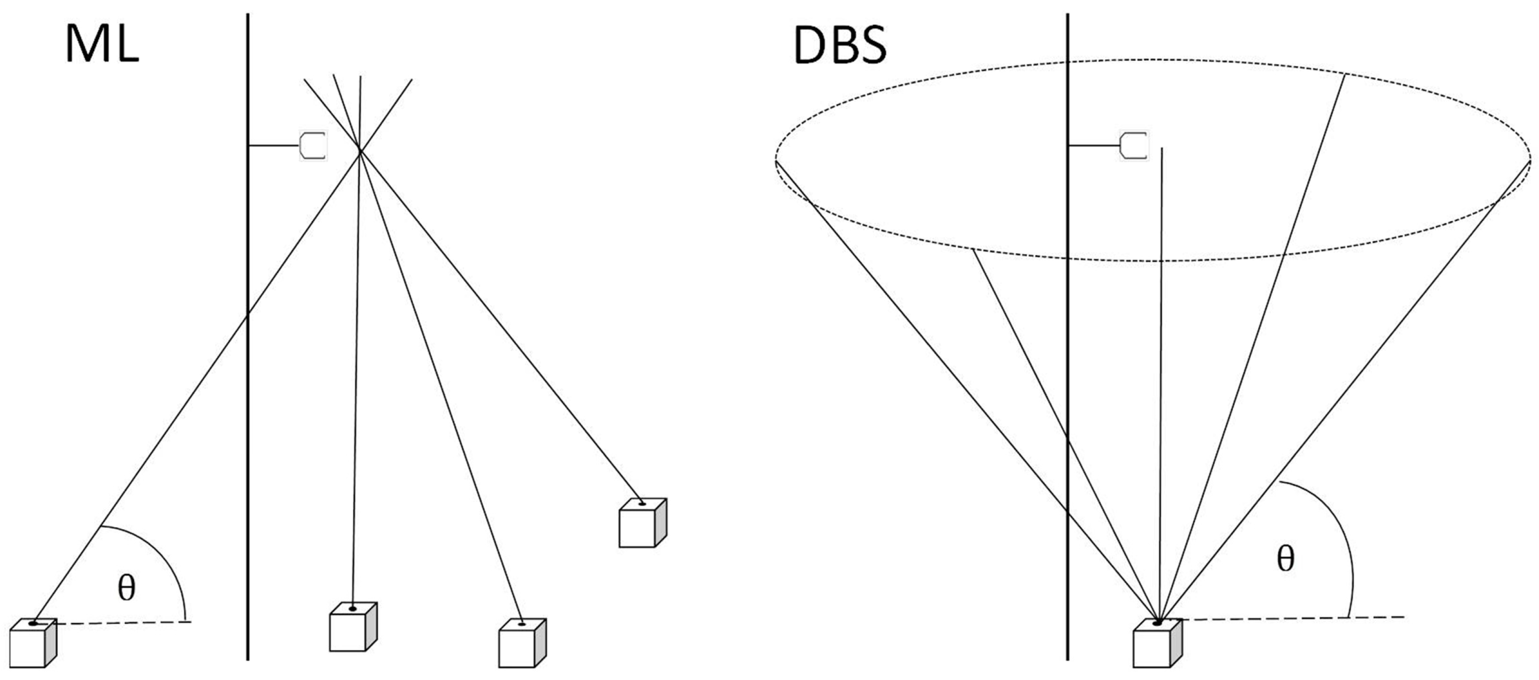
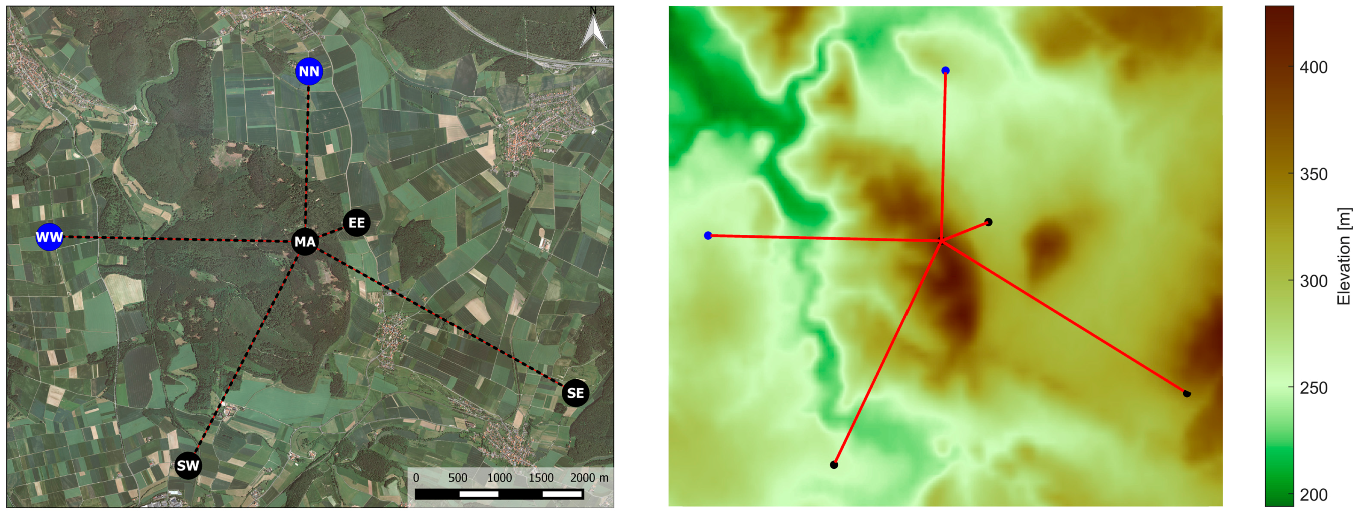
2.4. Experimental Setup: The Kassel 2014 Experiment

The data presented in this paper was collected during the Kassel 2014 Experiment at Rödeser Berg—a hill in central Germany close to Kassel—during summer 2014 (3 July–17 August 2014). Five long-range WindScanners (scanning lidars based on the Windcube WLS200s) were set up around the hill (EE, SE, SW, WW, NN in Figure 2). A sixth scanner (MA) was placed on the ridge of the hill directly next to a 200 m high meteorological mast. An additional Windcube v2 (DBS lidar) was operated at a few meters’ distance from the mast. The measurements from a sonic anemometer mounted on the mast serve as a reference in this study.

The reference mast is erected on a small clearance within a forest which, depending on direction, stretches from 0.4 to 2.5 km around the mast. The wider surroundings are characterised by a patchy landscape of mainly agricultural land use, villages and forested hills (Figure 2). The height of the hill above the surrounding terrain is approx. 100–200 m depending on direction. More details about the measurement site can be found in [6].

During the deployment of the WindScanners the procedures for calibration of the home position, levelling, and sensing range as outlined in [15] were applied. For the purpose of these procedures around each WindScanner, with the exception of the MA WindScanner, at distances of approx. 100 m, three 2 cm thick surveying stakes were installed, separated by 120° in azimuth. The absolute positions of the WindScanners, stakes, and reference mast top were surveyed using a differential GPS and a theodolite. These positions were acquired with cm accuracy. The stakes were then mapped using the CNR-Mapper [15]. After the calibration, the reference mast top was mapped by each WindScanner to validate the setup procedure, and the static laser beam pointing accuracy and the sensing range accuracy were estimated to be 0.05° and 1 m, respectively.

Due to the terrain configuration, reference mast structure and surrounding vegetation, the deployment steps, which are described above, could not be applied completely to the MA WindScanner. Hence, a single surveying stake and the branch of a tree nearby were used for the CNR mapping. Both hard targets were located about 50 m from the WindScanner and separated by 180° in azimuth. However, since the MA system was located directly next to the reference mast, the static pointing accuracy and sensing range accuracy could not be validated by mapping the mast top. The WindScanners were coordinated and synchronized by a remote master computer [15], which communicated with the WindScanners using a 3G network [32].

This paper analyses data from measurements when all WindScanners were staring at a single point close to a Gill HS50 sonic anemometer mounted on the reference mast at a height of 188 m (agl).

The reference anemometer is mounted on a foldable boom with a length of 5.4 m to minimise the effects of the mast structure. The wind sector 100°–160° is excluded from the analysis to remove data which is affected by the mast shadow. According to [2], the influence of the mast structure is estimated to be less than 0.5%. In a wind tunnel test the directional deviation of the Gill HS50 is well below ±1%. The inclinometer accuracy is given as ±0.15°. The direction-dependent error of the measurement of the horizontal wind speed is thus estimated to be below ±1%. The sampling frequency of the Gill HS50 was set to 50 Hz.

Although there is data from six available WindScanners, we restrict the analysis to four locations (EE, SW, SE and MA). These locations have the advantage that they have the longest time series in the analysed scanning mode. Details about the setup of the four scanners can be found in

Table 1. Overview of the lidar devices and locations which were used in this study. Coordinates are given in UTM Zone 32U. Pulse length and gate length are given as full width at half maximum (FWHM).

	MA	EE	SE	SW	WC
Instrument type	WLS 200S V2	WLS 200S	WLS 200S	WLS 200S V2	WINDCUBE WLS7 V2
Altitude (m)	387.7	294.6	346.6	258.3	387.7
Latitude (m)	5,690,182.6	5,690,409.1	5,688,371.9	5,687,503.8	5,690,181.2
Longitude (m)	513,590.5	514,213.3	516,843.2	512,185.9	513,593.1
$\mathsf{\theta }$ (°)	90	23.3	3.5	6.0	62, 90
$\mathsf{\psi }$ (°)	-	250.6	299.3	27.4	8, 98, 188, 278, -
Dist. to mast (m)	2	732	3740	3047	3
Pulse length FWHM (ns)	100	400	400	400	175
Gate length FWHM (ns)	74	150	150	150	58
${\sigma }_p$ (m)	6.4	25.5	25.5	25.5	11.1
${\sigma }_g$ (m)	9.5	19.1	19.1	19.1	7.4
Accumulation time (s)	2	2	2	2	~1.12 (~5.62 for full circle)

.

2.5. Data Treatment, Quality Control and Coordinate Systems

Quality control of lidar data is usually done by using a lower carrier-to-noise ratio (CNR) threshold to identify periods when not enough backscatter is received to derive a reliable wind-speed estimate. If a structure is present close to the measurement volume, returns from this hard target can also contaminate the signal. Often this leads to an increased CNR and/or to an increased scatter in the observed CNR values. Careful analysis of the WindScanner data, which was collected during the presented experiment, however, showed that also periods during which the CNR fell into the expected CNR range (here −27.5 and −5 dB were used) and had a “normal” variability sometimes exhibited spurious radial wind-speed statistics. Therefore, two additional filter criteria were imposed on the WindScanner data.

The first sorts the radial wind velocities of each averaging interval according to their magnitude. Outliers are then removed if the gap between them and the rest of the data exceeds 1 m·s⁻¹. This method is useful in situations with a relatively high radial velocity which is contaminated with hard target returns, as these are often characterised by a radial wind speed close to zero. The filter, however, becomes ineffective if the mean radial wind speed is close to zero—i.e., winds perpendicular to the lidar beam or low wind speeds. The second filter criterion therefore checks the time series during the averaging interval for its temporal consistency. If the time series after the application of the first filter still exhibits a difference between two adjacent measurements which exceeds 1 m·s⁻¹, the respective period is removed completely from further analysis. This threshold seems justified because of the relatively high sampling frequency (0.5 Hz) and the damping effect of the lidar probe volume on small-scale turbulence. The exact reason for the problems with the hard targets could not fully be clarified. At the beginning of the experiment, the WindScanners were focused within approx. 1 m above the reference sonic. The following points may then have led to interference with the mast structure: instability of the WindScanner systems (sinking into soil after installation, vibration of the systems due to e.g., wind), switching of the staring mode to other patterns inducing pointing error due to backlash of the internal gearing, and/or movement of the mast structure. For future inter-comparison experiments, it is thus recommended to increase the distance to the reference instrument/mast. The problem with the hard targets was not present in the data of the Windcube v2 and only a CNR filter was applied. The values (−22 and −5 dB) slightly differ from the WindScanners as the system configuration is different.

The analysis in this paper is based on 10 min averaging intervals, which is the standard in wind-energy applications. Before the analysis of the wind-vector components, a rotation into the mean wind direction ($\overline{v}=0 \mathrm{m}·{\mathrm{s}}^{-1}$) is performed. A second rotation forcing $\overline{w}=0 \mathrm{m}·{\mathrm{s}}^{-1}$ as done in many other micrometeorological studies (cf. [33]) is not carried out as the aim of the study is mainly a comparison of the different measurement techniques. For this same reason, corrections which are often applied to eddy-covariance measurements (cf. [34]), such as correcting for high- and low-frequency loss, are not applied to the sonic anemometer measurements. In a previous study, Mauder and co-authors reported deviations between a Gill HS and other sonic anemometers, which was attributed to the Gill HS [35]. However, in their study, the internal correction/calibration was turned off, which removes the sensor head correction and the instrument-dependent calibration. In the present study, the internal corrections were turned on and the problems reported in [35] are assumed to not to be present in the collected data.

3. Results and Discussion

3.1. Radial Velocity Components

In a first step, the radial components of the individual WindScanners ($v_{r lidar}$) are compared to the projection of the sonic measurement on the respective WindScanner beam ($v_{r sonic}$). This allows an evaluation of the performance of the individual instruments and the accuracy of the setup process. Moreover, some of the complexities in the inter-comparison of the second-order moments, which arise from the combination of multiple lidar beams in three-dimensional space, can be simplified when the radial components of the sonic and lidar wind speed are compared directly. In Section 3.2., we then turn to the wind statistics which are derived from the combination of multiple WindScanner devices.

3.1.1. First-Order Statistics

The inter-comparison of the mean radial components reveals an excellent agreement between the sonic and all WindScanner devices. A two-parametric linear regression between the WindScanners located around the mast and the reference sonic produces slopes ($m$) and intersects ($b$) which are very close to 1 and $0\mathrm{m}·{\mathrm{s}}^{-1}$ (

Table 2. Summary of the inter-comparison of the radial velocities of the WindScanners and the sonic anemometer at 188 m; RMSD indicates the root-mean-square deviation; R² is the goodness of the fit, $m$ is the slope and $b$ the intersect of the of the linear regression.

	MA	EE	SE	SW
No 10 min periods	503	2592	1419	1278
Mean $\overline{v_r}$
m	1.045	0.992	1.005	0.993
b (m·s−1)	0.056	−0.036	0.018	0.055
R2	0.858	0.999	0.998	1.000
RMSD (m·s−1)	0.087	0.104	0.116	0.079
Variance $\overline{v{\prime }_r^2}$
m	0.970	0.829	0.836	0.819
b (m·s−1)	0.017	−0.025	−0.018	0.001
R2	0.969	0.968	0.952	0.970

). The goodness of fit for the linear regression for these instruments is R² ≥ 0.998. The linear-regression statistics for MA are slightly worse. However, this instrument is pointing vertically into the atmosphere and $\overline{w}$ is usually small in the atmospheric boundary layer. In fact, ${\overline{v}}_{r MA}$ only varied between approx. $\pm 1\mathrm{m}·{\mathrm{s}}^{-1}$ and the root-mean-square deviation (RMSD) is comparable to the other WindScanners.

The availability of all WindScanners is affected by hard targeting (mast structure, boom or guying). As a result, the number of valid measurement periods, especially for the MA location, is relatively low. A conclusion on how the measurement range affects the data availability is therefore unfortunately not possible.

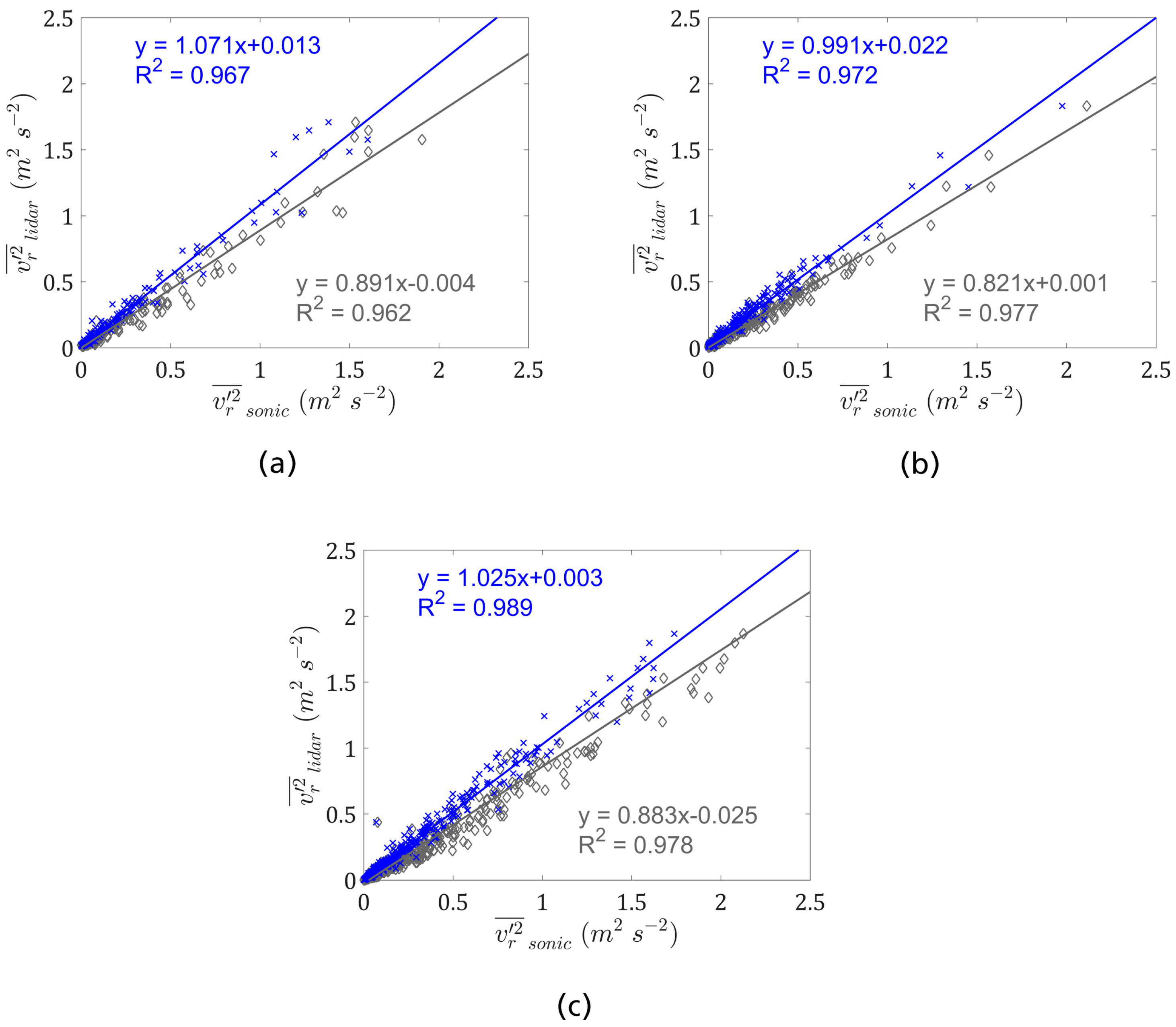
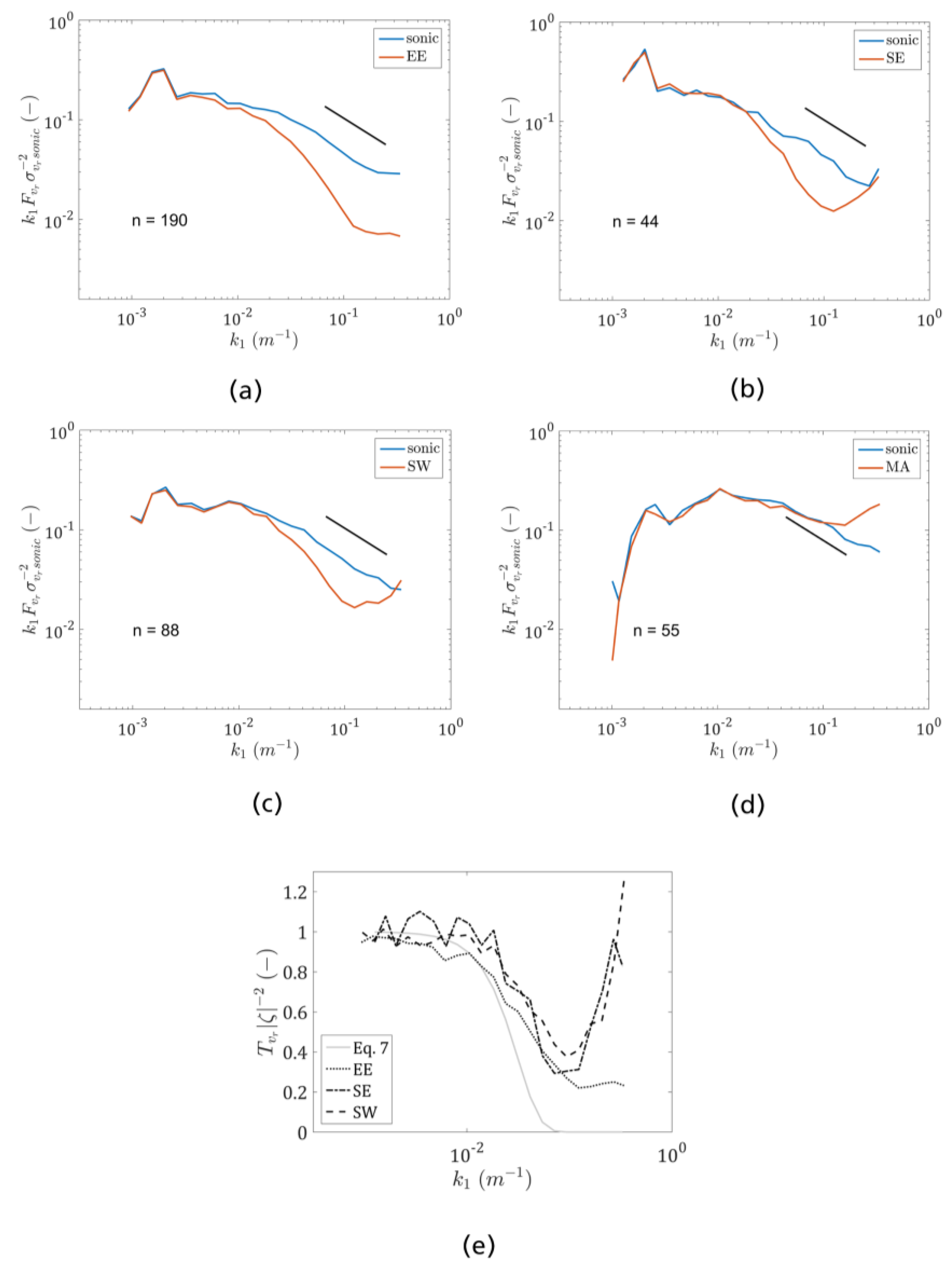
3.1.2. Second-Order Statistics

For the locations SE, SW and EE, the linear-regression statistics between ${\overline{v{\prime }_r^2}}_{lidar}$ (measured by the WindScanners) and the respective variance derived from the projection of the sonic measurement onto the direction of the respective WindScanner beam (${\overline{v{\prime }_r^2}}_{sonic}$) are very similar (Table 2). The slope indicates a significant underestimation of ${\overline{v{\prime }_r^2}}_{sonic}$ by the WindScanner measurements. This is likely to be due to the relatively large probe volume. In contrast, the slope of the linear regression for the MA system is significantly closer to 1. Here, the smaller range gate size seems to more than compensate for the smaller turbulent length scales which are usually found for $w$. R² is similar for all systems. The values are slightly worse than for the first-order statistics, except for the MA location, where R² is slightly higher. The reduced values in R² are probably partly caused by the reduced range of the observed variances when compared to the mean values. Another reason for the increased scatter is due to the fact that line averaging does not necessarily scale linearly with the observed variance. It is rather direction dependent on and selective of small wavenumbers. This makes the attenuation dependent on the form of ${\Phi }_{ij}\left(\mathit{k}\right)$ (9), which varies with atmospheric conditions—i.e., under stable conditions, a larger portion of the variance will be contained in small eddies as opposed to under unstable conditions. Also, since a finite time interval is used (10 min), some scatter will be introduced by the stochastic distribution of the eddy sizes in the individual period. To further investigate the probe-volume averaging effect on ${\overline{{v^{\prime }}_{r }^2}}_{lidar}$ periods with wind directions close to parallel (±15°) to the azimuth angle of the individual WindScanner beams, SE, SW and EE were selected. The spectral filter function defined by (7) and (10) was applied to $v_{r sonic}$ (Figure 3). The application of the filter function to the sonic data brings the slope of the linear regression between ${\overline{{v^{\prime }}_{r }^2}}_{sonic}$ and ${\overline{{v^{\prime }}_{r }^2}}_{lidar}$ closer to unity and slightly improves R² for all systems. Interestingly, this improvement is also observed for the EE system, which has quite a large inclination angle into the atmosphere ($\mathsf{\theta }$ = 22.3°).

A comparison of the average spectra of $v_r$ of the sonic and WindScanner measurements reveals a clear spectral attenuation for SE, SW and EE spectra from approx. $k_1>{10}^{-2} m^{-1}$ (Figure 4a–c). In contrast to the other systems, the spectrum of MA does not exhibit a clear spectral attenuation, which again is likely to be due to the smaller probe volume. Instead, the spectral energy at the high wavenumber tail for MA is actually higher than for the reference sonic. This behaviour can also be observed for the SW system (Figure 4c). Also $T_{v_r}$ starts to increase at appox. $k_1>{10}^{-1} {\mathrm{m}}^{-1}$ for all systems (Figure 4e). This effect becomes worse if measurements with small variances are included (data not shown) and is likely to be attributed to instrumental noise. The theoretical considerations (Equation 7) deviate from the observed shape and the attenuation only starts at wavenumbers higher than theoretically predicted for the SE and SW systems.

Up until now, only a few experimental studies investigating ${\overline{{v^{\prime }}_{r }^2}}_{lidar}$ and its spectrum against reference measurements have been undertaken. Most interesting in regards to pulsed lidars, Mann and co-authors [14] reported a good agreement between the observed and theoretical forms of $T_{v_r}$. However, in contrast to this study, they only used five selected periods and the lidars were set up in the direct vicinity of the reference mast. As this leads to large elevation angles, they had to use a spectral tensor model to derive $T_{v_r}$. Also, they used a simpler, triangular-shaped weighting function. The influence of measurement noise at the high-wave-number end of the spectra has also been reported for continuous wave lidars [36,37] and deserves further investigation for the WindScanner systems. Angelou et al. [36] found similar deviations between $T_{v_r}$ from theoretical considerations and $T_{v_r}$ computed from lidar and sonic spectra for a continuous wave lidar. As in the present investigation the reason for the deviation from theoretical considerations remains unclear. Nevertheless, Figure 4e indicates that the concept of line averaging (9 and 10) can be used to explain some of the differences in the observed second-order statistics between the sonic and the WindScanners.

3.2. Horizontal Wind-Speed Statistics from the ML and Doppler Beam Swinging (DBS) Technique

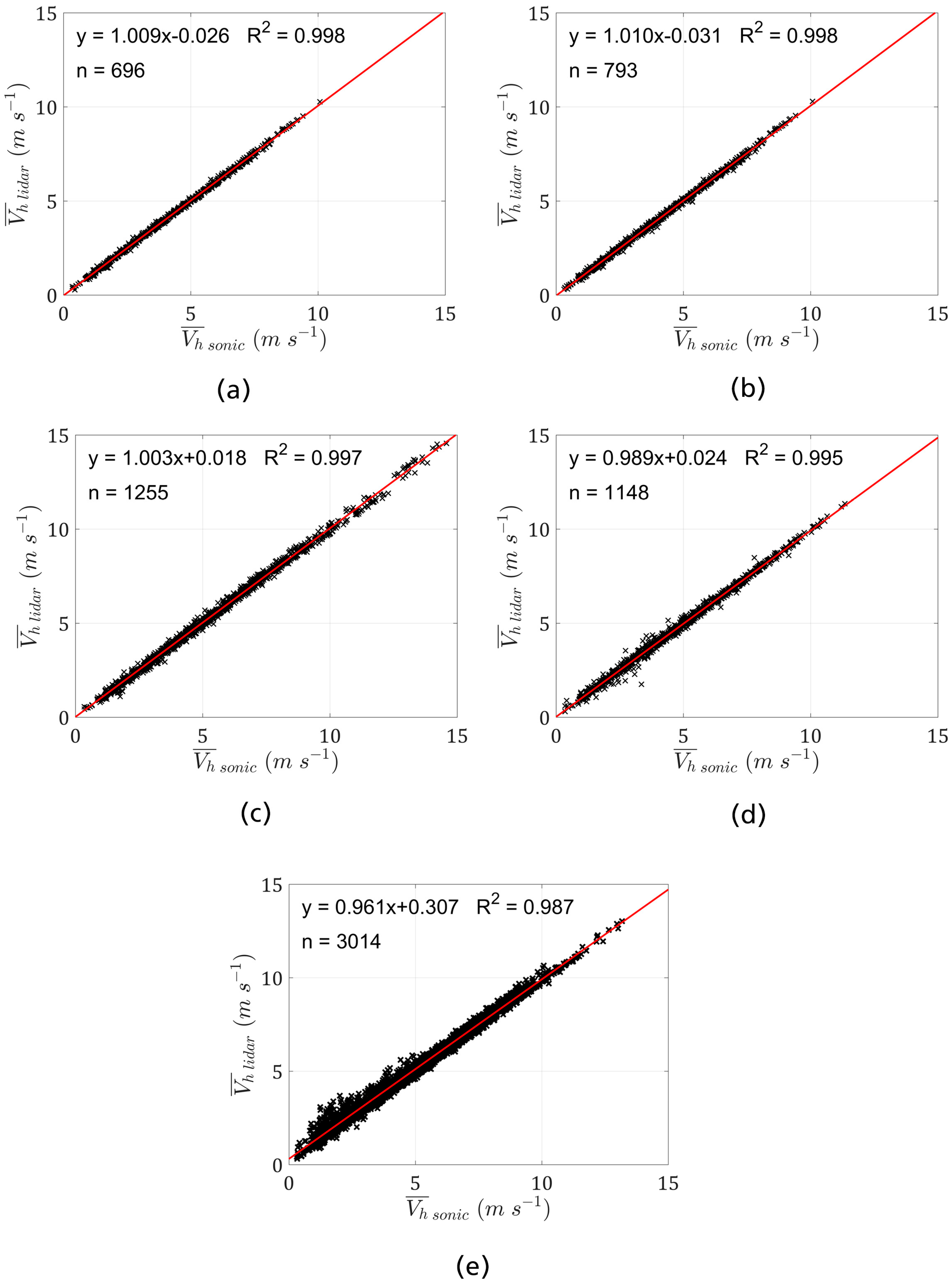
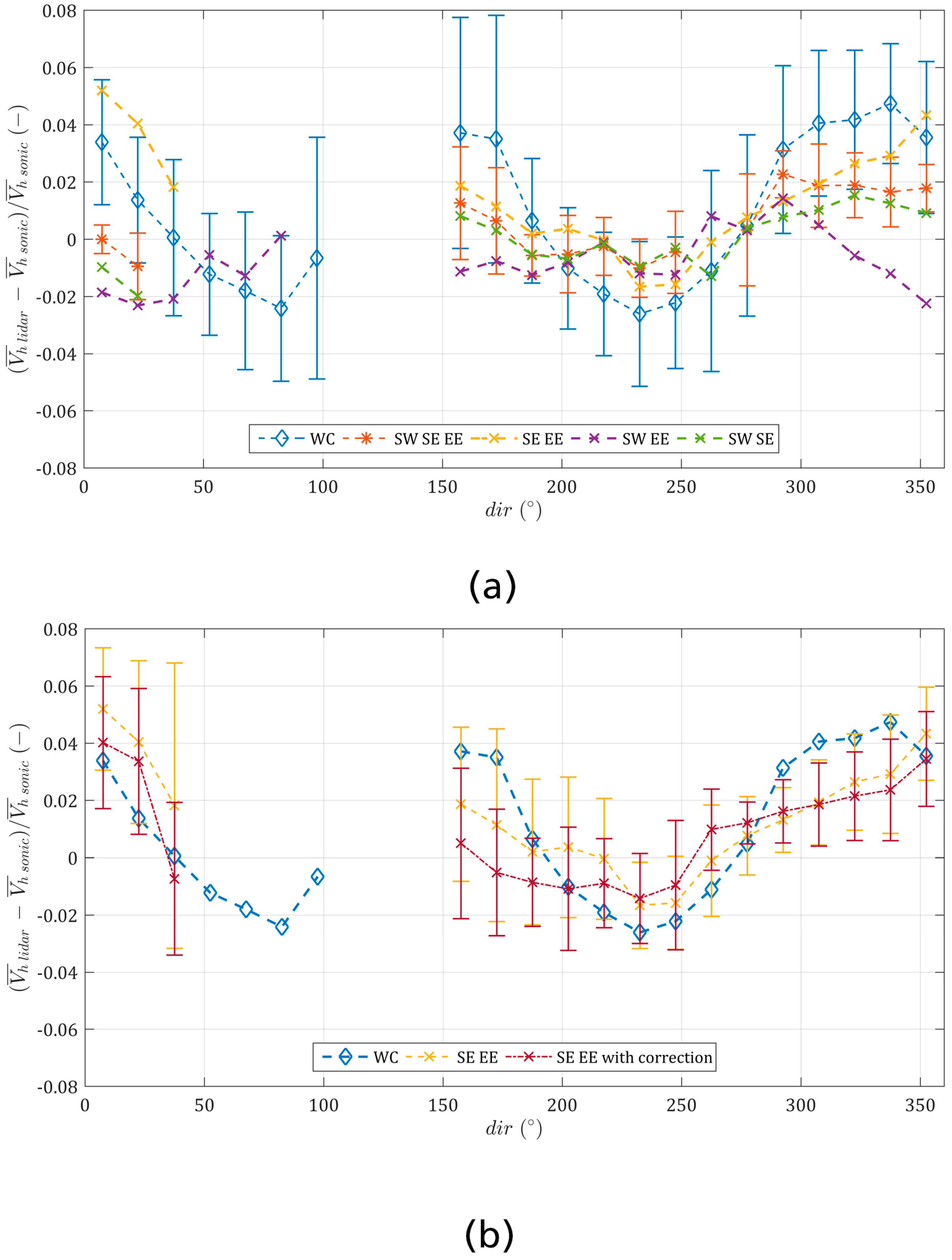
3.2.1. First-Order Statistics of the Horizontal Wind Speed

For resource estimation in the wind industry, it is standard to use the scalar horizontal velocity ($\overline{V_h}$). This approach is also followed here. Although in many remote sensing applications it is common practice to work with the vector average of the wind velocity, publications concerning the accuracy of lidars in complex terrain often use the scalar mean [4,6]. While vector averaging produces slightly different numbers, the general patterns that can be observed remain the same and the differences are very small.

The comparison of $\overline{V_h}$ measurements of the ML combination using three lidars and the sonic reveals an excellent agreement between the two techniques as would be expected from the comparison of $\overline{v_r}$ (Figure 5a). Also, the ML technique using two lidars and neglecting the vertical component in the vector reconstruction only produces marginally different results for the scanner combination SE/SW (Figure 5b). For the SW/EE combination, the scatter slightly increases and we can see a few points which significantly deviate from the linear relationship (Figure 5d). The observed differences between the different dual-lidar configurations are likely to be at least partly caused by the setup of the instruments.

One characteristic which sets the different dual-lidar measurements apart is the difference in azimuth angle between the WindScanner beams. For SW/EE, the angle is smallest (43°) which causes the strongest error propagation from the radial wind speed onto the wind vector when solving Equation (3) (cf. [38]). The angle for SE/EE is slightly larger (49°) and the SE/SW combination has an angle difference of 88°, which is close to the ideal 90°.

The DBS measurement with the Windcube v2 exhibits more scatter and the linear regression significantly deviates from 1:1 when compared to the sonic (Figure 5e). Especially for low wind speeds, an overestimation of the ${\overline{V_h}}_{sonic}$ by the DBS lidar can be observed.

In general, the linear-regression statistics for the DBS lidar are similar to what has been reported at Rödeser Berg in earlier measurement campaigns [6] and are similar to what has been reported from other lidar-mast inter-comparisons in complex terrain [39] albeit significantly worse than in flat terrain (e.g., [1]). In contrast, the statistics for the ML combinations are similar to the results which we regularly observe during DBS lidar calibrations in flat and homogeneous terrain. The “bump” in the DBS data at low wind speeds might be associated with turbulence effects which are more important for low wind speeds. Moreover, thermal effects on the flow might create increased vertical velocities (relative to the horizontal wind speed) which are likely to spatially vary in the complex surroundings at Rödeser Berg. In combination with the large scanning volume of the DBS lidar at 188 m this would introduce an increased complex terrain error.

To our knowledge no statistics from a comparably long-term data set for assessing the performance of ML measurements to derive the mean wind speeds have been published so far. Previously published results of mast-lidar inter-comparisons either focused on the evaluation of individual measurement periods [16] or employed scanning strategies that focused more on assessing the spatial heterogeneity of the wind field than on evaluating ML measurements against a reference [17,40]. The ML-mast inter-comparison in the latter two references is slightly worse, but due to the different focus of the scanning strategy, is likely to not be directly comparable. A recently published study by Newman only compares co-located DBS and ML measurements [19]. The sonic anemometer used in this study only measures at significantly lower altitudes than the lidars and is only used to give an indication of the wind field below the lidar measurements. This precludes a quantification of the advantages of either of the techniques over the other in their study or a comparison to the results presented.

One of the typical observations for profiling lidars in complex terrain is that the deviation in $\overline{V_h}$ between the lidar and the mast measurements varies with the shape of the terrain and thus wind direction [4,6]. This behaviour can also be observed for the DBS data collected during the Kassel Experiment 2014 (Figure 6). The pattern clearly reflects the shape of the terrain and is very similar to what has been observed in earlier inter-comparisons between cup anemometers and a DBS lidar at Rödeser Berg [6]. If the flow is directed across the ridge of the hill (aprox. 50°–100° and 200°–270°), the DBS lidar underestimates $\overline{V_h}$. This is a typical observation for convex flow as observed over e.g., ridges or hilltops [4,5]. In contrast, the sectors showing an overestimation of $\overline{V_h}$ by the DBS lidar (approx. 290°–20° and 160°–180°) correspond to along the ridge flow. Here, the mast is located on the slope in front of/behind the highest point on the ridge and the terrain is slightly concave. This might also cause a concave flow pattern which results in an overestimation of the horizontal wind speed by the DBS lidar. Some evidence for this can be found in the change of sign of the flow angle measured by the sonic between 290°–20° and 160°–180°. Whereas for the first sector (mast in front of the hill top) the median flow angle is 1.7° (directed upwards), it is −2.2° (directed downwards) for the second sector (mast behind the hill top). It should be noted, however, that the real flow might be more complex than this simplified explanation. A more detailed discussion and modelling results of directional errors of DBS lidar measurements at Rödeser Berg can be found in [6].

On average, the DBS-mast deviations are slightly shifted (1%–2%) towards an increased ${\overline{V_h}}_{lidar}$ (relative to ${\overline{V_h}}_{sonic})$ when compared to the earlier inter-comparison to cup anemometry. This might be caused by the different reference anemometers or the different DBS instruments used in the present study, although the reason could not be fully clarified.

The deviation between ${\overline{V_h}}_{lidar}$ and ${\overline{V_h}}_{mast}$ for the ML measurements is smaller than for the DBS system for most sectors and WindScanner combinations (Figure 6). Especially for the WindScanner combinations SW/SE/EE and SE/SW, the differences are small for all directions and only vary between approx. −2% and 2%. For the SE/EE combination, a relatively large positive deviation of the ML system in comparison to the sonic wind speed can be observed between approx. 350 and 25°, which even exceeds the DBS-sonic deviations. This is likely due to the fact that within this range, the angle between the mean wind direction and the beam directions of SE and EE are large and the difference in beam directions is small (cf. [38]). This configuration leads to an increased error propagation in the estimation of $u$ that largely dominates ${\overline{V_h}}_{lidar}$—i.e., the azimuth angles and flow direction are unfavourable for the retrieval of ${\overline{V_h}}_{lidar}$. For flow angles which are directed in a more parallel manner to the orientation of the lidar beams, the error propagation for $v$ is expected to be large. The effect on ${\overline{V_h}}_{lidar}$, however, is then much smaller.

A second effect which can affect the quality of the measurements of SE/EE combination is the relatively large elevation angle of the EE system compared to the other systems (Table 1). The assumption, $\overline{w}=0 \mathrm{m}·{\mathrm{s}}^{-1}$, thus results in a contamination of ${\overline{V_h}}_{lidar}$ by $\overline{w}$. Due to the low availability, an inclusion of the MA system which could correct for the influence of $\overline{w}$ in the directional analysis was not possible. Therefore, a direction-dependent correction factor was calculated using ${\overline{w}}_{sonic}$. Equation (3) is first solved using ${\overline{v}}_{r SE}$, ${\overline{v}}_{r EE}$ and ${\overline{w}}_{sonic}$. In a second step, (3) is solved only using ${\overline{v}}_{r SE}$ and ${\overline{v}}_{r EE}$. The ratio of the two results is then applied as a correction factor to ${\overline{V_h}}_{lidar}$. The correction reduces the deviations in the 350°–25° sector. The effect is, however, relatively small. Therefore, the assumption $\overline{w}=0 \mathrm{m}·{\mathrm{s}}^{-1}$ does not seem to be the main cause of the observed deviations. Some of the deviations between the sonic and the lidar measurements might also be caused by the flow distortion of the mast. However, we estimate this effect to be small (c.f. Section 2.4.).

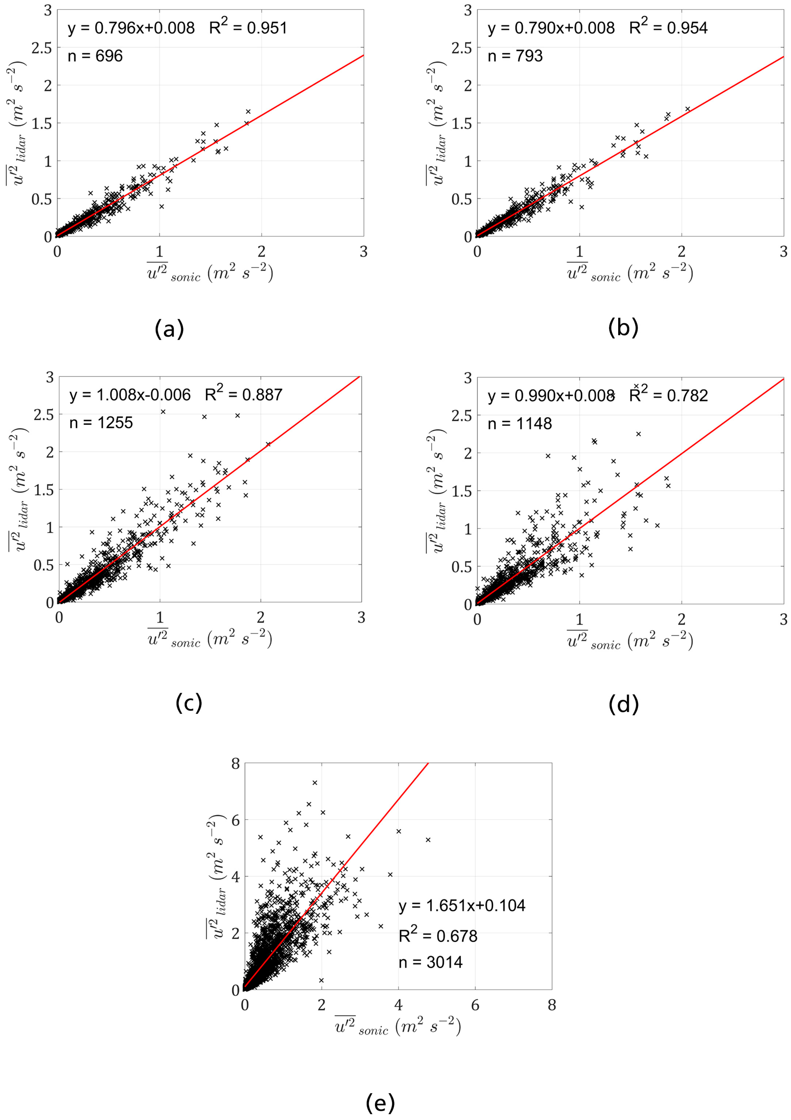
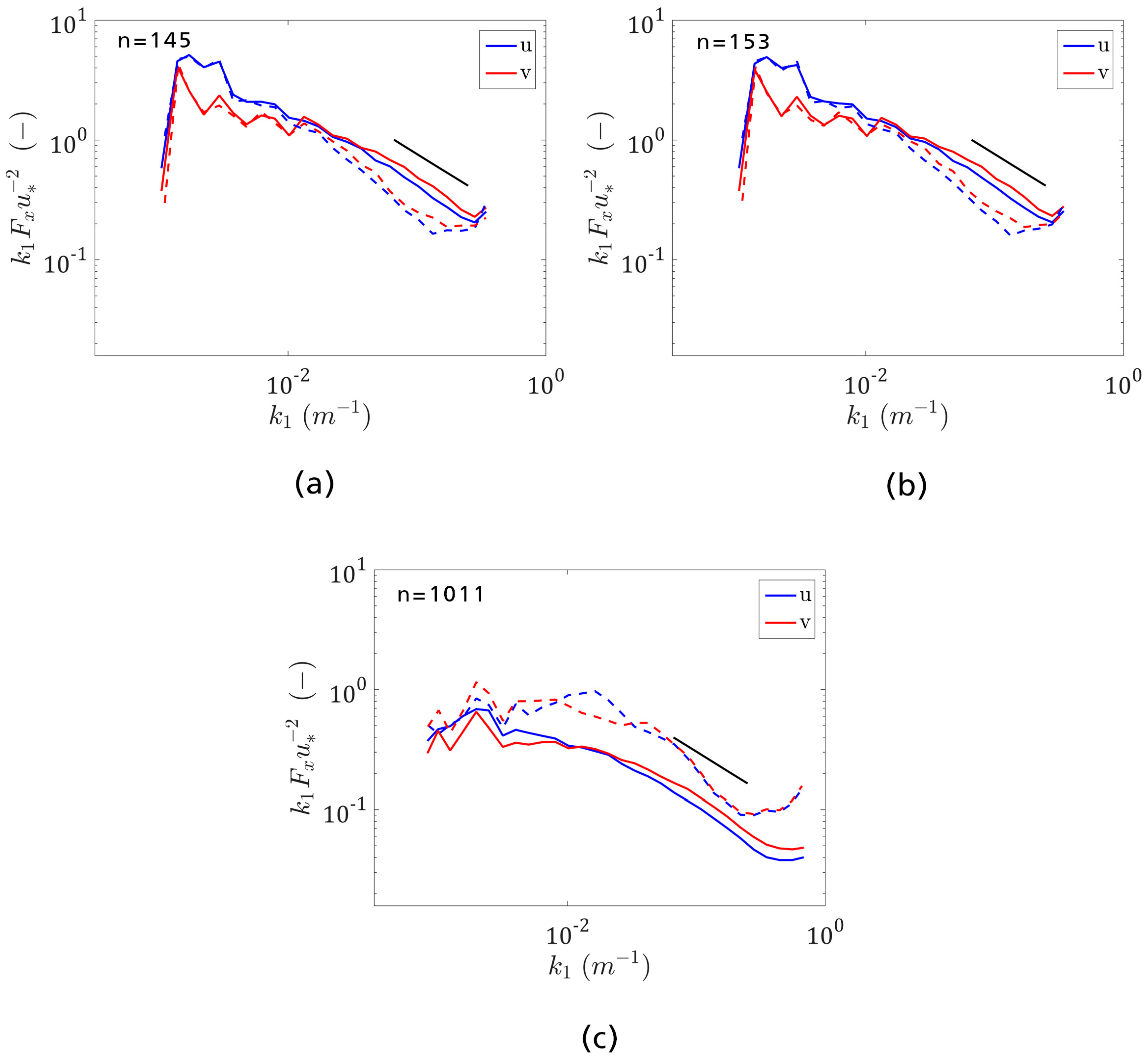
3.2.2. Second-Order Statistics of the Horizontal Wind Vector Components

This section presents the second-order statistics (variances and spectra) of the horizontal wind components $u$ and $v$. The second-order statics for the $w$ component can be found in Section 3.1.2. (MA WindScanner). Figure 7 displays the scatter plots and linear-regression statistics for the different ML combinations and the DBS lidar when compared to the sonic measurements. The differences between the DBS and ML, but also among the different ML combinations, are quite large. Almost identical linear-regression statistics can be observed for the SW/SE/EE and SW/SE combinations (Figure 7a,b). The R² values of the linear regression for $\overline{u^{\prime 2}}$ and $\overline{v^{\prime 2}}$ are similar to the statistics of $\overline{{v^{\prime }}_{r }^2}$ (Table 2 and Figure 3). Also the slope indicates a similar underestimation of $\overline{u^{\prime 2}}$ (and $\overline{v^{\prime 2}}$) of about 20%. Looking at the spectra of SW/SE/EE and SW/SE, one can clearly see the effects of line averaging which causes the reduction in $\overline{u^{\prime 2}}$ and $\overline{v^{\prime 2}}$ (Figure 8a,b). As for $v_r$, an attenuation in the spectral density from approx. $k_1={10}^{-2} {\mathrm{m}}^{-1}$ for $u$ and $v$ can be observed. The line averaging effect thus also causes the reduced $\overline{u^{\prime 2}}$ and $\overline{v^{\prime 2}}$ in SW/SE/EE and SW/SE.

The scatter in the inter-comparison between the SW/EE and SE/EE is larger than for SW/SE/EE and SW/SE and the slope of the linear regression shifts close to 1. One of the reasons for the increased scatter in the ML combinations using two WindScanners including the EE system might be that the EE system has an inclination angle which is not close to 0°. In the wind-vector reconstruction for two scanners, the $w$ component is assumed to be 0 m·s⁻¹. Some of $\overline{w^{\prime 2}}$ will thus contaminate the measurement of $\overline{u^{\prime 2}}$ and $\overline{v^{\prime 2}}$. Moreover, as discussed earlier, the direction of the flow in relation to the beam directions will also influence the error propagation for the individual components, especially if the angle between the beams is small [38]. In the experimental setup it is, however, difficult to separate these effects as they are likely to be correlated.

This observation suggests that for the ML method, an adequate positioning of the lidar devices is even more important for measuring turbulence quantities than for the mean wind speed.

In general, random measurement errors in the time series will always lead to an increased variance. Therefore, both the contamination by the $w$ component and the unfavourable angles in the lidar combination lead to increased $\overline{u^{\prime 2}}$ and $\overline{v^{\prime 2}}$ in the lidar measurement. The slope values close to the 1:1 line are thus likely a result of the combination of these measurement errors and the line averaging, which act in opposing directions.

The comparison between the DBS system and the sonic indicates a clear overestimation of $\overline{u^{\prime 2}}$ and $\overline{v^{\prime 2}}$ by the DBS system (Figure 7e and

Table 3. Summary of the linear-regression statistics for $\overline{u^{\prime 2}}$ and $\overline{v^{\prime 2}}$ for different lidar configurations; values in brackets are statistics for which periods with ${\overline{u}}_{sonic}<4 \mathrm{m}·{\mathrm{s}}^{-1}$ have been excluded; R² is the goodness of the fit, $m$ is the slope and $b$ the intersect of the of the linear regression.

	SE SW EE	SW SE	SE EE	SW EE	WC
$\overline{\mathit{u}{\prime }^{\mathbf{2}}}$
m	0.796 (0.829)	0.790 (0.816)	1.008 (1.026)	0.990 (0.916)	1.651 (1.531)
b (m·s−1)	0.008 (0.006)	0.008 (0.009)	−0.006 (-0.011)	0.008 (0.006)	0.104 (0.070)
R2	0.951 (0.963)	0.954 (0.967)	0.887 (0.896)	0.782 (0.865)	0.678 (0.796)
$\overline{\mathit{v}{\prime }^{\mathbf{2}}}$
m	0.825 (0.800)	0.822 (0.800)	0.884 (0.861)	0.883 (0.890)	1.822 (1.731)
b (m·s−1)	0.003 (0.008)	0.004 (0.009)	-0.006 (-0.007)	0.020 (0.018)	0.076 (0.038)
R2	0.962 (0.963)	0.966 (0.966)	0.903 (0.930)	0.861 (0.901)	0.689 (0.737)

). Also, the R² values are lower than for all ML combinations. The spectra of the DBS system show a significant contamination of the variance measurements across almost the whole wavenumber range. Only for very large $k_1$ are the spectra for the $u$ component of the DBS lidar and the sonic close together. For the $u$ component, a local maximum can be observed around approx. $k_1={10}^{-1.8} {\mathrm{m}}^{-1}$. The $v$ spectrum of the DBS lidar is higher than the sonic spectrum for the whole wave number range and a (smaller) second maximum can be observed around $k_1={10}^{-1.4} {\mathrm{m}}^{-1}$. For higher wave numbers, the spectra then quickly drop off.

The exact shape of the measured spectra of a Windcube does not only depend on the atmospheric conditions and measurement heights, but will also vary with the flow direction towards the scanning geometry of the Windcube [10]. It is thus difficult to explain all features of the measured spectra.

The strong positive deviations from the sonic spectra in this range are likely to be caused by the cross-contamination effects between $\overline{u^{\prime 2}}$, $\overline{v^{\prime 2}}$ and especially by the contamination of the horizontal variances by $\overline{w^{\prime 2}}$. The short region where the spectra are almost horizontal at the high wavenumber end is likely to be caused by the algorithm which derives the wind vector from the measurements of $v_r$. In analogy with the internal software of the Windcube v2, in this paper the wind vector was calculated whenever a new measurement of $v_r$ was available—i.e., at a frequency of approx. 0.89 Hz. One full rotation, however, takes five measurements of $v_r$ and thus acts similarly to a moving average filter [41].

The relatively strong overestimation in the measured variances by the Windcube compared to some other studies using similar instruments (Windcube v1 and v2) [9,19] is likely to be related to the great measurement height (188 m) and thus the large distance between the different beams. In parts, it might also be caused by a dominance of unstable conditions which are more frequent during the summer season and the inhomogeneous flow caused by the terrain complexity.

In Table 3, we also provide the statistics for periods when ${\overline{u}}_{sonic}>4\mathrm{m}·{\mathrm{s}}^{-1}$, as this filter criterion is often used in applications and studies in the wind-energy sector, thereby allowing a more direct comparison to other experiments. For the ML combinations SW/SE/EE, SW/SE and SE/EE, there is only a small change in the linear-regression statistics. For the Windcube v2 and the SW/EE, which have lower R² values, R² significantly improves after the application of the ${\overline{u}}_{sonic}>4 \mathrm{m}·{\mathrm{s}}^{-1}$ criterion.

4. Conclusions

Two of the biggest challenges for ground-based remote sensing in wind energy are the systematic errors in the mean wind speed which can be introduced by complex flow in complex terrain and the inability of traditional profiling devices to accurately measure turbulence. This paper experimentally explores the improvements in these two areas which can be made using the multi-lidar (ML) technique. For this purpose, results from the Kassel 2014 Experiment are presented, during which multiple WindScanners and a Doppler beam swinging (DBS) lidar were operated surrounding a reference mast in complex terrain.

The comparison of the radial wind velocities between the WindScanner measurements and a reference sonic shows that, given an accurate setup, an excellent agreement with the reference sonic could be achieved for individual systems, even if they are positioned several kilometres from the mast. Combination of multiple lidars to an ML measurement demonstrate that this also holds true for the derivation of the horizontal wind speed. ML wind speeds were considerably closer to the mast reference than the DBS lidar at this complex terrain site. The significantly reduced scatter and the smaller directional deviation in comparison with the reference sonic clearly demonstrate the advantages of focusing multiple lidar beams at one point over the classical DBS-profiling method. Correction methods (based on e.g., flow models) can be avoided, which can significantly reduce the uncertainty in applications like wind resource assessments or site calibrations. Exploiting the flexibility of the WindScanner technology, the measurements presented here could be extended to a scan of multiple measurement locations within a planned windfarm site. Especially in complex terrain this could significantly reduce the uncertainty associated with the horizontal extrapolation of the wind resource. For research applications like flow model validation, the ML technique removes the constraints of a mast measurement for an accurate measurement of the horizontal wind speed.

The ML measurements of $\overline{{v^{\prime }}_{r }^2}$, $\overline{u{\prime }^2}$ and $\overline{v{\prime }^2}$ (for SW/SE/EE and SW/SE) showed a high correlation to the reference sonic. However, while larger scale turbulence was accurately captured, due to the relatively large measurement volume and the associated path averaging, attenuation for higher wave numbers could be observed. This results in an overall underestimation of the variances. An obvious way forward would be to reduce the measurement volume. With currently available lidar technology, however, this comes at the cost of a reduced measurement range and, therefore, reduces the flexibility of ML measurements. An alternative is to develop correction methods for the variance which is lost due to the line averaging. First-order corrections could be based on model spectra as often done for eddy-covariance measurements (e.g., [42]). The spectral transfer function, however, needs further attention. Alternatively, the correction could be based on an extrapolation of the spectra in the inertial sub-range [43,44]. This, however, requires that a part of the inertial sub-range is not affected by line averaging. More sophisticated approaches could exploit e.g., the spectral broadening of the received backscatter [25,45,46]. The results for the variance measurements of the DBS lidar clearly illustrate the errors introduced by cross-contamination in this technique and reiterate the unreliability of turbulence measurements from profiling lidars.

From a practical perspective, it is interesting that the good results of the ML method could also be maintained if only two lidars were used. This reduces the additional costs, which are one of the disadvantages of the ML method, when compared to the DBS lidar (or other profiling lidar). Differences between the different dual-lidar ML systems are likely to be mainly caused by the setup or, more precisely, the different angles between the WindScanners. While the mean wind speed is only slightly affected, the variances of the horizontal wind-speed components seem to be more sensitive to an unfavourable setup of the WindScanners. A detailed analysis of the effect of the setup on the accuracy of ML measurements is part of ongoing investigations.

References

1. Gottschall, J.; Courtney, M.S.; Wagner, R.; Jørgensen, H.E.; Antoniou, I. Lidar profilers in the context of wind energy—A verification procedure for traceable measurements. Wind Energy 2012, 15, 147–159. [Google Scholar] [CrossRef]
2. International Electrotechnical Commission. IEC 61400-12 Wind Turbines—Part 12-1: Power Performance Measurements of Electricity Producing Wind Turbines (2nd Committee Draft), 2nd ed.; International Electrotechnical Commission: Geneva, Switzerland, 2013. [Google Scholar]
3. Fördergesellschaft Windenergie und andere Erneuerbare Energien e.V. (FGW). TR6 Bestimmung von Windpotenzial und Energieerträgen. Available online: http://www.wind-fgw.de/TR.html (accessed on 20 September 2016).
4. Bingöl, F.; Mann, J.; Foussekis, D. Conically scanning lidar error in complex terrain. Meteorol. Z. 2009, 18, 189–195. [Google Scholar] [CrossRef]
5. Bradley, S.; Strehz, A.; Emeis, S. Remote sensing winds in complex terrain—A review. Meteorol. Z. 2015, 24, 547–555. [Google Scholar]
6. Klaas, T.; Pauscher, L.; Callies, D. Lidar-mast deviations in complex terrain and their simulation using CFD. Meteorol. Z. 2015, 24, 591–603. [Google Scholar]
7. Sathe, A.; Mann, J. A review of turbulence measurements using ground-based wind lidars. Atmos. Meas. Tech. 2013, 6, 3147–3167. [Google Scholar] [CrossRef] [Green Version]
8. Sathe, A.; Banta, R.; Pauscher, L.; Vogstad, K.; Schlipf, D.; Wylie, S. Estimating Turbulence Statistics and Parameters from Ground- and Nacelle-Based Lidar Measurements; IEA Wind Expert Report; DTU Wind Energy: Roskilde, Denmark, 2015. [Google Scholar]
9. Sathe, A.; Mann, J.; Gottschall, J.; Courtney, M.S. Can wind lidars measure turbulence? J. Atmos. Ocean. Technol. 2011, 28, 853–868. [Google Scholar] [CrossRef]
10. Sathe, A.; Mann, J. Measurement of turbulence spectra using scanning pulsed wind lidars. J. Geophys. Res. 2012, 117. [Google Scholar] [CrossRef] [Green Version]
11. Newman, J.F.; Klein, P.M.; Wharton, S.; Sathe, A.; Bonin, T.A.; Chilson, P.B.; Muschinski, A. Evaluation of three lidar scanning strategies for turbulence measurements. Atmos. Meas. Tech. 2016, 9, 1993–2013. [Google Scholar] [CrossRef]
12. Sathe, A.; Mann, J.; Vasiljevic, N.; Lea, G. A six-beam method to measure turbulence statistics using ground-based wind lidars. Atmos. Meas. Tech. 2015, 8, 729–740. [Google Scholar] [CrossRef] [Green Version]
13. Eberhard, W.L.; Cupp, R.E.; Healy, K.R. Doppler lidar measurement of profiles of turbulence and momentum flux. J. Atmos. Ocean. Technol. 1989, 6, 809–819. [Google Scholar] [CrossRef]
14. Mann, J.; Cariou, J.-P.; Courtney, M.S.; Parmentier, R.; Mikkelsen, T.; Wagner, R.; Lindelöw, P.; Sjöholm, M.; Enevoldsen, K. Comparison of 3D turbulence measurements using three staring wind lidars and a sonic anemometer. Meteorol. Z. 2009, 18, 135–140. [Google Scholar] [CrossRef]
15. Vasiljevic, N. A Time-Space Synchronization of Coherent Doppler Scanning Lidars for 3D Measurements of Wind Fields. Ph.D. Thesis, Technical University of Denmark, Roskilde, Denmark, 2014. [Google Scholar]
16. Fuertes, F.C.; Iungo, G.V.; Porté-Agel, F. 3D turbulence measurements using three synchronous wind lidars: Validation against Sonic Anemometry. J. Atmos. Ocean. Technol. 2014, 31, 1549–1556. [Google Scholar] [CrossRef]
17. Berg, J.; Vasiljevíc, N.; Kelly, M.; Lea, G.; Courtney, M. Addressing spatial variability of surface-layer wind with long-range WindScanners. J. Atmos. Ocean. Technol. 2015, 32, 518–527. [Google Scholar] [CrossRef]
18. Mann, J. The spatial structure of neutral atmospheric surface-layer turbulence. J. Fluid Mech. 1994, 273, 141–168. [Google Scholar] [CrossRef]
19. Newman, J.F.; Bonin, T.A.; Klein, P.M.; Wharton, S.; Newsom, R.K. Testing and validation of multi-lidar scanning strategies for wind energy applications. Wind Energy 2016. [Google Scholar] [CrossRef]
20. Mann, J.; Angelou, N.; Arnqvist, J.; Callies, D.; Cantero, E.; Chávez Arroyo, R.; Courtney, M.; Cuxart, J.; Dellwik, E.; Gottschall, J.; et al. Complex terrain experiments in the New European Wind Atlas. Philos. Trans. R. Soc. A 2016. in review. [Google Scholar]
21. Tatarskii, V.I.; Muschinski, A. The difference between Doppler velocity and real wind velocity in single scattering from refractive index fluctuations. Radio Sci. 2001, 36, 1405–1423. [Google Scholar] [CrossRef]
22. Huffaker, R.M.; Hardesty, R.M. Remote sensing of atmospheric wind velocities using solid-state and CO2 coherent laser systems. Proc. IEEE 1996, 84, 181–204. [Google Scholar] [CrossRef]
23. Frehlich, R. Effects of wind turbulence on coherent Doppler lidar performance. J. Atmos. Ocean. Technol. 1997, 14, 54–75. [Google Scholar] [CrossRef]
24. Lindelöw, P.J.P.; Mohr, J.J.; Peucheret, C.; Feuchter, T.; Christensen, E.L. Fiber Based Coherent Lidars for Remote Wind Sensing; Technical University of Denmark, DTU: Kgs. Lyngby, Denmark, 2008. [Google Scholar]
25. Banakh, V.A.; Smalikho, I.N. Estimation of the turbulence energy dissipation rate from the pulsed Doppler lidar data. Atmos. Ocean. Opt. 1997, 10, 957–965. [Google Scholar]
26. Kaimal, J.C.; Wyngaard, J.C.; Haugen, D.A. Deriving power spectra from a three-component sonic anemometer. J. Appl. Meteorol. 1968, 7, 827–837. [Google Scholar] [CrossRef]
27. Cariou, J.-P.; Leopshere, Paris, France. Personal communication, 2016.
28. International Electrotechnical Commission. IEC 61400-1 Wind Turbines—Part 1: Design Requirements; International Electrotechnical Commission: Geneva, Switzerland, 2005. [Google Scholar]
29. Veers, P.S. Three-Dimensional Wind Simulation; Sandia National Laboratories: Albuquerque, NM, USA, 1988. [Google Scholar]
30. Mann, J. Wind field simulation. Probab. Eng. Mech. 1998, 13, 269–282. [Google Scholar] [CrossRef]
31. Farr, T.G.; Rosen, P.A.; Caro, E.; Crippen, R.; Duren, R.; Hensley, S.; Kobrick, M.; Paller, M.; Rodriguez, E.; Roth, L.; et al. The shuttle radar topography mission. Rev. Geophys. 2007, 45. [Google Scholar] [CrossRef]
32. Vasiljevic, N.; Lea, G.; Hansen, P.; Jensen, H.M. Mobile Network Architecture of the Long-Range WindScanner System; DTU Wind Energy: Roskilde, Denmark, 2016. [Google Scholar]
33. Kaimal, J.C.; Finnigan, J.J. Atmospheric Boundary Layer Flows: Their Structure and Measurement; Oxford University Press: New York, NY, USA, 1994. [Google Scholar]
34. Foken, T.; Leuning, R.; Oncley, S.R.; Mauder, M.; Aubinet, M. Corrections and data quality control. In Eddy Covariance: A Practical Guide to Measurement and Data Analysis; Aubinet, M., Vesala, T., Papale, D., Eds.; Springer Netherlands: Dordrecht, The Netherlands, 2012; pp. 85–131. [Google Scholar]
35. Mauder, M.; Oncley, S.P.; Vogt, R.; Weidinger, T.; Ribeiro, L.; Bernhofer, C.; Foken, T.; Kohsiek, W.; de Bruin, H.; Liu, H. The energy balance experiment EBEX-2000. Part II: Intercomparison of eddy-covariance sensors and post-field data processing methods. Bound. Lay Meteorol. 2007, 123, 29–54. [Google Scholar] [CrossRef]
36. Angelou, N.; Mann, J.; Sjöholm, M.; Courtney, M. Direct measurement of the spectral transfer function of a laser based anemometer. Rev. Sci. Instrum. 2012, 83, 033111. [Google Scholar] [CrossRef] [PubMed] [Green Version]
37. Sjöholm, M.; Mikkelsen, T.; Mann, J.; Enevoldsen, K.; Courtney, M. Spatial averaging-effects on turbulence measured by a continuous-wave coherent lidar. Meteorol. Z. 2009, 18, 281–287. [Google Scholar] [CrossRef]
38. Stawiarski, C.; Träumner, K.; Knigge, C.; Calhoun, R. Scopes and challenges of dual-Doppler lidar wind measurements — an error analysis. J. Atmos. Ocean. Technol. 2013, 30, 2044–2062. [Google Scholar] [CrossRef]
39. Bradley, S.; Perrott, Y.; Behrens, P.; Oldroyd, A. Corrections for wind-speed errors from sodar and lidar in complex terrain. Bound. Lay. Meteorol. 2012, 143, 37–48. [Google Scholar] [CrossRef]
40. Newsom, R.K.; Berg, L.K.; Shaw, W.J.; Fischer, M.L. Turbine-scale wind field measurements using dual-Doppler lidar. Wind Energy 2015, 18, 219–235. [Google Scholar] [CrossRef]
41. Canadillas, B.; Bégué, A.; Neumann, T. Comparison of turbulence spectra derived from Lidar and sonic measurements at the offshore platform FINO1. In Proceedings of the 10th German Wind Energy Conference (DEWEK 2010), Bremen, Germany, 17–18 November 2010.
42. Moore, C.J. Frequency response corrections for eddy correlation systems. Bound. Lay. Meteorol. 1986, 37, 17–35. [Google Scholar] [CrossRef]
43. Hogan, R.J.; Grant, A.L.M.; Illingworth, A.J.; Pearson, G.N.; O’Connor, E.J. Vertical velocity variance and skewness in clear and cloud-topped boundary layers as revealed by Doppler lidar. Q. J. R. Meteorol. Soc. 2009, 135, 635–643. [Google Scholar] [CrossRef]
44. Barlow, J.F.; Halios, C.H.; Lane, S.E.; Wood, C.R. Observations of urban boundary layer structure during a strong urban heat island event. Environ. Fluid Mech. 2015, 15, 373–398. [Google Scholar] [CrossRef]
45. Smalikho, I.; Köpp, F.; Rahm, S. Measurement of atmospheric turbulence by 2-μm Doppler lidar. J. Atmos. Ocean. Technol. 2005, 22, 1733–1747. [Google Scholar] [CrossRef]
46. Mann, J.; Peña, A.; Bingöl, F.; Wagner, R.; Courtney, M.S. Lidar scanning of momentum flux in and above the atmospheric surface layer. J. Atmos. Ocean. Technol. 2010, 27, 959–976. [Google Scholar] [CrossRef]
Figure 1. Sketch of the multi-lidar (ML) and Doppler beam swinging (DBS) strategies next to a reference mast with a sonic as used in this study. Note that the angles and positions of the lidars differ from the instrument setup for reasons of illustrative clarity.
Remotesensing 08 00782 g001
Figure 2. Instrumental setup during the measurement campaign. Left: aerial photograph (data source: published with kind permission of ©Hessische Verwaltung für Bodenmanagement und Geoinformation (HVBG)) with circles indicating the locations of the lidar and the met mast; the locations which are used in this study are indicated in black. Right: terrain (data source: Shuttle Radar Topography Mission [31] version 2.1) and trajectories of the intersecting lidar beams for the ML measurement. The windcube v2 (WC) is also located at the MA position.
Remotesensing 08 00782 g002
Figure 3. Variance of the radial velocity measurements of the WindScanners ( v r   2 ¯ l i d a r ) against the respective variance in the direction of the beam derived from the sonic anemometer ( v r   2 ¯ s o n i c ) when the wind direction was close to parallel (±15°) to the azimuth angle of the WindScanner for (a) SE; (b) SW; (c) EE; grey diamonds indicate the unfiltered sonic measurements; blue crosses are the sonic data after the application of (10). The sonic data was filtered with | ζ ^ ( k 1 ) | 2 to separate out the effects of the temporal averaging.
Remotesensing 08 00782 g003
Figure 4. Spectra of v r measured by different WindScanners and the sonic anemometer when the wind direction was close to parallel (±15°) to the azimuth angle of the WindScanner (ac); (d) spectra of the MA location and the w component of the sonic anemometer; sonic time series have been aggregated to 0.5 Hz before calculation of the spectra to account for the temporal averaging effect and the associated filter function ζ ^ ( k 1 ) ; the black line indicates the theoretical −2/3-slope in the inertial subrange; (e) spectral transfer function | ζ ^ | 2 T v r derived from the average of the normalised spectra in (ac); only periods with u ¯ s o n i c > 4   m · s 1 and u 2 ¯ s o n i c > 0.2   m 2 · s 2 (SW, SE, EE), and w 2 ¯ s o n i c > 0.1   m 2 · s 2 (MA) were used in the spectral averaging; n indicates the number of periods used for averaging.
Remotesensing 08 00782 g004
Figure 5. Scatter plots of V h ¯   from different lidar configurations against the reference sonic at 188 m; (a) SE/SW/EE; (b) SE/SW; (c) SE/EE; (d) SW/EE; (e) Windcube v2 next to the mast; (ad) are measurements from WindScanners in ML mode; the Windcube in (e) is operated in DBS mode. For ML combinations with only two beams, w = 0   m · s 1 is assumed in the wind-vector reconstruction; n indicates the number of value pairs displayed in the individual scatter plots.
Remotesensing 08 00782 g005
Figure 6. (a) mean of the directional deviation in V h ¯   between the sonic and the different lidar configurations; (b) same as (a) but for the SE/EE combination with and without the correction for w ¯ ; see text for details; periods during which V h ¯   s o n i c < 4   m · s 1 were excluded from the comparison to increase the comparability to other complex terrain measurements reported in the literature. Also, bins with n < 5 are not displayed; error bars denote ± one standard deviation.
Remotesensing 08 00782 g006
Figure 7. Scatter plots of u 2 ¯   from different lidar configurations against the reference sonic at 188 m; (a) SE, SW and EE; (b) SE and SW; (c) SE and EE; (d) SW and EE; (e) Windcube v2 next to the mast; (ad) are measurements from WindScanners in ML mode; the Wincube is operated in DBS mode. For ML combinations with only two beams, w = 0   m · s 1 is assumed in the wind-vector reconstruction; n indicates the number of value pairs displayed in the individual scatter plots.
Remotesensing 08 00782 g007
Figure 8. Normalised spectra of u and v . For (a) SW/SE/EE, (b) SW/SE and (c) Windcube v2 next to the mast; solid lines are the sonic spectra; dashed lines are the lidar spectra; sonic time series have been aggregated to 0.5 Hz (a and b) and 0.89 Hz before calculation of the spectra; only periods with u ¯ s o n i c > 4   m · s 1 and u 2 ¯ s o n i c > 0.2   m 2 · s 2 were used in the spectral averaging; u * is the friction velocity computed from the sonic anemometer measurements; the black line indicates the theoretical −2/3 slope in the inertial subrange; n indicates the number of periods used for averaging.
Remotesensing 08 00782 g008