Satellite Based Mapping of Ground PM_2.5 Concentration Using Generalized Additive Modeling

Abstract

Satellite-based PM_2.5 concentration estimation is growing as a popular solution to map the PM_2.5 spatial distribution due to the insufficiency of ground-based monitoring stations. However, those applications usually suffer from the simple hypothesis that the influencing factors are linearly correlated with PM_2.5 concentrations, though non-linear mechanisms indeed exist in their interactions. Taking the Beijing-Tianjin-Hebei (BTH) region in China as a case, this study developed a generalized additive modeling (GAM) method for satellite-based PM_2.5 concentration mapping. In this process, the linear and non-linear relationships between PM_2.5 variation and associated contributing factors, such as the aerosol optical depth (AOD), industrial sources, land use type, road network, and meteorological variables, were comprehensively considered. The reliability of the GAM models was validated by comparison with typical linear land use regression (LUR) models. Results show that GAM modeling outperforms LUR modeling at both the annual and seasonal scale, with obvious higher model fitting-based adjusted R² and lower RMSEs. This is confirmed by the cross-validation-based adjusted R² with values of GAM-based spring, summer, autumn, winter, and annual models, which are 0.92, 0.78, 0.87, 0.85, and 0.90, respectively, while those of LUR models are 0.87, 0.71, 0.84, 0.84, and 0.85, respectively. Different to the LUR-based hypothesis of the “straight line” relations, the “smoothed curves” from GAM-based apportionment analysis reveals that factors contributing to PM_2.5 variation are unstable with the alternate linear and non-linear relations. The GAM model-based PM_2.5 concentration surfaces clearly demonstrate their superiority in disclosing the heterogeneous PM_2.5 concentrations to the discrete observations. It can be concluded that satellite-based PM_2.5 concentration mapping could be greatly improved by GAM modeling given its simultaneous considerations of the linear and non-linear influencing mechanisms of PM_2.5.

1. Introduction

As a primary air pollutant in most cities in China, fine particulate matter with an aerodynamic diameter less than 2.5 µm (PM_2.5) have been associated with significant adverse impacts on ecological environment and public health (e.g., respiratory problems, cardiovascular and lung diseases) [1,2,3,4]. According to the Global Burden of Disease 2010 Study [5], over 1.2 million people lost lives in China due to exposure to outdoor PM_2.5, accounting for 38% of the total number caused by ambient particulate matter pollution worldwide. Thus, accurately understanding the space–time distributions and associated dynamic variations of PM_2.5 concentrations is urgently needed to provide a scientific basis for the effective prevention and control of PM_2.5-related health risk.

Remote sensing was initially employed to estimate the ground-level PM_2.5 concentrations based on satellite-retrieved aerosol optical depth (AOD) almost three decades ago [6,7,8]. Attributed to the superiority in large spatial coverage and relatively lower cost, satellite-based mapping of ground PM_2.5 concentration has, therefore, become an increasingly prominent solution, recently, to complement the ground measurements of sparse regular stationary monitoring sites [9]. In this process, some typical statistical models have been developed, such as land use regression (LUR) models and geographically-weighted regression (GWR) models based on LUR. While these models can integrate the AOD, auxiliary meteorological and geographical parameters (e.g., land use data) to estimate PM_2.5 concentration with an acceptable accuracy [10,11,12], most of them depend on the presumed linear relationships between the measured PM_2.5 concentrations and certain influencing factors. As a result, the inherent complex chemical and physical influencing mechanisms between PM_2.5 and impacting factors are totally ignored in modeling. These are usually considered by the chemical transport model [13]. However, the chemical transport model approach is very demanding in computing time and memory, which seriously limits its use in large problems. Therefore, a simplified empirical statistical model is recommended for PM_2.5 estimation with high resolution, which can relax the linearity constraint between variables and, meanwhile, consider the effect of both emission sources and dispersion conditions without intensive computations.

As a popular nonlinear modeling method, generalized additive modeling (GAM) is able to capture the highly non-linear and non-monotonic relationships between variables. Compared with model-driven methods, GAM is more like a data-driven method. The relationships between variables in GAM models are determined by the data themselves, instead of being pre-assumed. Due to its successful applications in spatial pattern simulation and driving factors identification in ecological modeling [14,15], the GAM approach has been gradually applied in air quality modeling studies. The results indicate that the flexible nonlinear structure offered by GAM might better represent the potential relationships between wide-range PM_2.5 concentrations and predictors, though dispersion and chemical reaction are not only nonlinear in space [11,16,17,18].

However, as these reported studies were almost conducted in specific sites or cities with limited geographical extent, the possibility of the GAM approach in reflecting the spatial heterogeneity characteristics of PM_2.5 concentrations from a global or holistic perspective is still unclear. Meanwhile, the predictor variables’ contributions to PM_2.5 concentrations also lack detailed recognition. Additionally, these studies were mostly based on a single time scale, hence the temporal fluctuations of GAM models’ performance in estimating PM_2.5 concentrations are not fully taken into account. In other words, explanatory covariates and their associations with PM_2.5 concentrations may vary with changing time scales, and this implies the necessity of evaluating the stability and sensitivity of GAM modeling in estimating PM_2.5 concentrations over the time scale.

In this study, we therefore attempted to develop a GAM method for satellite based PM_2.5 concentration mapping by simultaneously considering the linear and non-linear relationships between PM_2.5 variation and associated contributing factors by taking the Beijing-Tianjin-Hebei (BTH) region as a case. The overall objective of this research was, to explore the applicability of the nonparametric GAM modeling in dealing with the nonlinearity of predictor variables; to evaluate the temporal sensitivity of GAM models at multiple time scales; as well as to identify the driving mechanism of prominent contributing factors to PM_2.5 concentrations. The results will be significantly instructive to deeply understand the formation and variation process of ground PM_2.5 concentrations and would be strongly supportive to the satellite based spatial distribution mapping of PM_2.5 concentrations.

2. Data and Methods

2.1. Study Area

The Beijing-Tianjin-Hebei (BTH) region is an urban agglomeration located in the Northern China, covering the entire Beijing municipality, Tianjin municipality and Hebei province (latitude range (36°05′N–42°37′N), longitude range (113°11′E–119°45′E)) (Figure 1). With the long history of industrial development and urban expansion, the BTH region has become one of the most polluted regions in China [19,20]. Frequent foggy and hazy weather with extremely high PM_2.5 concentrations over this region has attracted increasing worldwide attention [21]. It has been reported that the major sources of PM_2.5 in the BTH region are industrial emissions, coal combustion, vehicle exhausts, dust, biomass burning, and secondary sources [22,23]. Studies have shown that unfavorable topographical and meteorological factors (e.g., temperature, wind speed, humidity, and precipitation), as well as human activities (e.g., industrial production, traffic emissions, and other pollutant emission related activities in daily life) greatly contribute to the formation and variation of PM_2.5 pollution in this region [24,25].

2.2. Data Collection and Preprocessing

According to previous remote sensing-based research findings [9,26,27], the data that could be used as potential covariates to predict PM_2.5 concentrations in this study are AOD, PM_2.5 emissions-related data, such as pollution sources, road networks, land use/cover, population, as well as dispersion condition data, including meteorological parameters and terrain data.

2.2.1. In Situ PM_2.5 Data

Hourly PM_2.5 concentrations (μg/m³) in one year (1 June 2013–30 May 2014) observed at 78 monitoring sites in the BTH region were collected from the official website of China Environmental Monitoring Center (CEMC) (http://106.37.208.233:20035/). The ground-measured hourly PM_2.5 concentrations were monitored using the tapered element oscillating microbalance method (TEOM). To assure the validity of data, a strict validation procedure was conducted using a quality control criterion according to the Chinese National Ambient Air Quality Standards (CNAAQS). All missing or invalid data due to instrument malfunctions were removed from the original data, for example, the same measurement repeatedly reported for several successive hours, significantly larger measurements, or measurements with less than 20 records a day. After this, approximately 95% of the original 658,045 records were kept. The seasonal average and annual average PM_2.5 concentrations were then calculated for each station based on these quality-controlled hourly data and prepared as the dependent variable for the modeling followed.

2.2.2. Satellite-Retrieved AOD Data

As the most validated, accessible, and accurate dataset today [28,29], the daily level 2 (L2) AOD products (Collection 5.1) with a 10 km spatial resolution from Terra and Aqua MODIS (Moderate Resolution Imaging Spectroradiometer) were downloaded from the Atmospheric Archive and Distribution System (LAADS Web; http://ladsweb.nascom.nasa.gov/) over the time period of 1 June 2013–30 May 2014. These AOD data at 550 nm wavelength in the Collection 5.1 was retrieved by algorithms of dark target (DT) or dark blue (DB) overland [30]. The C005 MODIS-derived aerosol products were compared to global sunphotometer (AERONET) data with 85,463 valid MODIS/AERONET collocations (at 0.55 μm), and >66% (one standard deviation) fell within an expected error (EE) envelope of ±(0.05 + 15%) over land [31]. In this process, only the AOD data with the best quality assurance confidence flag (flag = 3) was employed and averaged as the daily AODs to minimize the influence of the AOD inaccuracy. The overall mean value of AODs (unitless) during the one-year study period was 0.36 with values ranging from 0.08 to 0.74. To reduce the negative influence of cloud on the quality of MODIS images and AODs in the study domain, we fitted a linear regression to define the relationship between the Terra MODIS AOD (MOD04) and the Aqua MODIS AOD (MYD04). We used this regression to predict the missing AOD value (i.e., predict MOD04 with the available MYD04, and vice versa), then MOD04 and MYD04 were averaged as the daily AOD if both of them were available [27,32]. Finally, all the remediated AODs were transformed to seasonal and annual average to improve spatial coverage.

2.2.3. PM_2.5 Emissions Related Data

To accurately simulate PM_2.5 concentrations without data in regional emission inventory, the pollution sources, road network, land use/cover, and population data, are employed to indirectly characterize the PM_2.5 emissions in this study, which possibly depict the industrial production or surface dust, vehicle exhaust, and other daily life-related emission sources.

In the national geographic conditions monitoring of the BTH region in 2013, pollution sources data associated with the rise of PM_2.5 concentrations, including fine-scale ground dust surfaces and locations of industrial plants, were captured. Ground dust surfaces were classified into the open pit field, stacked substance, construction site, natural bare surface, crush stampede yard, and others. Industrial plants were classified into the iron and steel smelting and rolling processing plants, thermal power plants, heat production and supply plants, cement building materials plants, petrochemical plants, non-ferrous metal smelting and processing plants, coal mining plants, paper and paper products plants, and pharmaceutical manufacturing plants. Road network data of 2013 referring to the traffic emissions were clipped from the national road network of China (http://ngcc.sbsm.gov.cn). Roads included in this study are expressway, national, provincial, county, and urban roads. Land use/cover data at a 30-m resolution in 2013 from the Chinese Geographical Information Monitoring Cloud Platform (http://www.dsac.cn/ServiceCase/Detail/10502) were reclassified into the built-up, forest, grasslands, waterbody, and others. The 1 km grid-based population data in 2013 was collected from the Center for Resources and Environmental Sciences, Chinese Academy of Sciences (RESDC) (http://www.resdc.cn).

2.2.4. Dispersion Conditions Data

Variation of ambient PM_2.5 concentration is not only influenced by PM_2.5 emission sources referenced in Section 2.2.3, but can be more affected by dispersion conditions such as meteorological and topography conditions, which have been proved by several previous studies [33,34]. Thus, meteorological data and topography conditions data are included into the model structure in this study.

The daily surface meteorological parameters were downloaded from the China Meteorological Data Sharing Service System (http://cdc.cma.gov.cn/), including temperature, wind speed, relative humidity, atmospheric pressure, and precipitation, from 26 Global Telecommunication System (GTS) stations distributed across the BTH region in the study period. Corresponding to the time scales of preprocessed PM_2.5 data, the mean values of temperature, wind speed, relative humidity, pressure, and the sum values of precipitation was preprocessed at the annual and seasonal scale for each monitoring sites. In this process, a strict data quality check procedure was conducted using a quality control method according to the Chinese National Meteorological Information Center (CNMC). Additionally, the DEM covering the BTH region with a resolution of 90 m produced by NASA was downloaded from USGS (http://www2.jpl.nasa.gov/srtm/dataprod.htm).

2.2.5. Data Integration

For data integration, the characteristic values of all these potential predictors were collected or preprocessed at the seasonal and annual scale from the measurements. They were extracted at each PM_2.5 stationary monitoring site and prepared as the modeling inputs of ArcGIS 10.3 software. In this process, the meteorological parameters with ground-based measurements were spatially interpolated to the fine grid of 10 km, which corresponds to the grid resolution of AOD datasets. For predictors with spatial scaling effects (e.g., land use/cover), the characteristic values were extracted at a 500–5000 m buffering radius based on previous findings [35,36]. Finally, PM_2.5, fused AOD, meteorological parameters, pollution sources, road network, land use/cover, terrain, and population for all PM_2.5 monitoring sites were matched by PM_2.5 monitoring site IDs for model development. Detailed information of the potential predictor variables can be found in

Table 1. Potential predictor variables for GAM and LUR modeling.

GIS Dataset	Predictor Variables		Unit	Buffer Size (m)
AOD	AOD		unitless	NA
Meteorological parameters	Temperature		K	NA
	Wind speed		m/s	NA
	Relative humidity		%	NA
	Atmospheric pressure		hPa	NA
	Precipitation		mm	NA
Pollution sources	Percentage of ground dust area in a buffer	Open pit field	%	500, 1000, 2000, 3000
		Stacked substance	%	500, 1000, 2000, 3000
		Construction site	%	500, 1000, 2000, 3000
		Natural bare surface	%	500, 1000, 2000, 3000
		Crush stampede yard	%	500, 1000, 2000, 3000
		Else	%	500, 1000, 2000, 3000
	Number of industrial plants in a buffer	Iron and steel smelting and rolling processing plants	count	400, 600, 800, 1000, 2000, 30,000
		Thermal power plants	count	400, 600, 800, 1000, 2000, 30,000
		Heat production and supply plants	count	400, 600, 800, 1000, 2000, 30,000
		Cement building materials plants	count	400, 600, 800, 1000, 2000, 30,000
		Petrochemical plants	count	400, 600, 800, 1000, 2000, 30,000
		Non-ferrous metal smelting and processing plants	count	400, 600, 800, 1000, 2000, 30,000
		Coal mining plants	count	400, 600, 800, 1000, 2000, 30,000
		Paper and paper products plants	count	400, 600, 800, 1000, 2000, 30,000
		Pharmaceutical manufacturing plants	count	400, 600, 800, 1000, 2000, 30,000
	Distance to the nearest industrial plants	Iron and steel smelting and rolling processing plants	m	NA
		Thermal power plants	m	NA
		Heat production and supply plants	m	NA
		Cement building materials plants	m	NA
		Petrochemical plants	m	NA
		Non-ferrous metal smelting and processing plants	m	NA
		Coal mining plants	m	NA
		Paper and paper products plants	m	NA
		Pharmaceutical manufacturing plants	m	NA
Road network	Length of all roads in a buffer		m	50, 60, 70, 80, 90, 100, 150, 250, 300, 350, 400, 450, 500, 1000, 1500, 2000, 2500, 3000, 3500, 4000, 4500, 5000
Land use/cover	Percentage of built-up area in a buffer		%	500, 1000, 1500, 2000, 2500, 3000, 3500, 4000, 4500, 5000
	Percentage of forests area in a buffer		%	500, 1000, 1500, 2000, 2500, 3000, 3500, 4000, 4500, 5000
	Percentage of grasslands area in a buffer		%	500, 1000, 1500, 2000, 2500, 3000, 3500, 4000, 4500, 5000
	Percentage of water area in a buffer		%	500, 1000, 1500, 2000, 2500, 3000, 3500, 4000, 4500, 5000
Terrain	DEM elevation		m	NA
Population	Population density		count	NA

NA = not available.

.

2.3. GAM Modeling

2.3.1. GAM Structure

GAM is a semi-parametric extension of the generalized linear model (GLM) with assumed additive functions and smooth components [37]. Generally, a generalized additive model in the context of using an identity link function with a Gaussian error distribution to estimate PM_2.5 concentration can be expressed as follows:

$$\begin{array}{ll}P{M}_{2.5,s}& ={\beta }_{0,s}+g\left(AO{D}_s\right)+g\left(Meteorologicalparameter{s}_s\right)+g\left(Pollutionsource{s}_s\right)\\ & +g\left(Roadnetwor{k}_s\right)+g\left(Landuse/cove{r}_s\right)+g\left(Terrai{n}_s\right)+g\left(Populatio{n}_s\right)\end{array}$$

where, s is the unique identify number of PM_2.5 monitoring sites, PM_2.5,s is the estimation of seasonal or annual average PM_2.5 concentration serving as the dependent variables of a site s, and AOD_s, Meteorological parameters_s, Pollution sources_s, Road network_s, Land use/cover_s, Terrain_s, and Population_s are independent variables at the corresponding site. β_0,s is the model intercept; g( ) is the smooth function to be estimated for predictor variables.

2.3.2. Thin Plate Regression Splines

Thin plate splines provide a general solution to the problem of estimating the smooth function “g( )” of multiple predictor variables [38]. The thin plate regression spline approach has turned out to be the optimal approximations to the thin plate splines with the considerable practical advantage of greatly enhanced computational efficiency and stability [39]. It can be used to efficiently incorporating multidimensional smoothers into GAMs in a manner that allows statistically well-founded model selection for such models. In this study the non-linear relationships were fitted with thin plate regression splines using automatically optimized smoothing parameters by the method of generalized cross-validation (GCV) as implemented by Wood’s R package “mgcv” [40].

2.3.3. Model Development and Validation

We chose an automatic forward-backward stepwise variable selection procedure (step-wise GAM procedure) to select the best fitting GAM models. This step algorithm uses the Akaike information criterion (AIC) statistic, taking into account both the information explained by the model and its complexity to evaluate models [41]. The final GAMs presented in this article are determined based on the criteria of the lowest AIC value and the highest adjusted R². A significance test was also conducted using the 0.05 level to check whether each term remaining in the finalized model was statistically significant. Furthermore, fitted relationships between PM_2.5 concentrations and particular linear or non-linear predictor variables were visualized using partial response plots and marginal effects. The overall fit of a GAM model was measured using a summary of adjusted fitting R² and root mean square error (RMSE) between the estimated PM_2.5 concentrations and observed ones. Considering the varying meteorological conditions and anthropogenic emissions, GAM models for seasonal and annual datasets were separately developed in this study.

Furthermore, we used a 10-fold cross-validation (10-CV) [42] to test the potential overfitting of the established GAM models. To be more detailed, the dataset was randomly divided into 10 folds, among which one fold was selected as the validation set and the remaining folds were the training sets. Predictions of the validation set were generated using those GAM models obtained through fitting the training set and the auxiliary data. This process was repeated 10 times until all samples were tested, and then the overall fit R² values and RMSEs between the estimated PM_2.5 concentrations and remaining observed ones are employed as the validation statistics. Meanwhile, these overall fit R² values and RMSEs were further compared with those from traditional LUR models developed based on the simple linear regression using the same datasets. We also compared the seasonal and annual averages of in situ PM_2.5 concentrations from 78 monitoring sites with the annual and seasonal mean predicted PM_2.5 concentrations based on the GAMs in both model fitting and validating. Additionally, in order to visually illustrate the fine variations of PM_2.5 concentrations within the BTH region, grid point-based predictions of annual and seasonal mean PM_2.5 concentrations at a spatial resolution of 10 km (including 2022 points) were estimated using the final robust GAM models and, consequently, employed to produce the continuous raster surfaces of PM_2.5 concentrations in ArcGIS 10.3.

3. Results

3.1. Model Fitting and Validation

As showed in

Table 2. Predictor variables for GAM and LUR models.

	GAM Models Established	LUR Models Established
Spring (N = 78)	PM2.5 ≈ s(AOD) + s(WS) + s(TEMP) + s(RH)	PM2.5 ≈ AOD + WS + TEMP + RH
Summer (N = 78)	PM2.5 ≈ AOD + s(FOR(5000 m)) + s(BUI(5000 m)) + s(TEMP)	PM2.5 ≈ AOD + TEMP + PRE
Autumn (N = 78)	PM2.5 ≈ s(AOD) + s(WS) + s(ELEV) + s(GD(3000 m))	PM2.5 ≈ AOD + PREC + WS + GD(3000 m)
Winter (N = 78)	PM2.5 ≈ s(AOD) + s(CS(2000 m)) + s(TEMP) + WS	PM2.5 ≈ AOD + TEMP + WS + CS(2000 m)
Annual (N = 78)	PM2.5 ≈ s(AOD) + s(TEMP) + s(GRA(5000 m)) + s(SS(2000 m)) + WS + PRE	PM2.5 ≈ AOD + WS + GD(3000 m) + PM(600 m)

Significant with p < 0.05; N is the total amount of the records in compared pairs; AOD = Aerosol Optical Depth; WS = wind speed; TEMP = temperature; RH = relative humidity; PRE = atmospheric pressure; GD = percentage of all ground dust area; CS = percentage of construction site area; SS = percentage of stacked substance area; BUI = percentage of built-up area; FOR = percentage of forests area; GRA = percentage of grasslands area; ELEV = elevation; PM = number of papermaking plant.

, seasonal and annual mean PM_2.5 and matched predictors were fitted at 78 monitoring sites (N = 78) using the GAM model and the traditional LUR model, respectively. All of the predictors listed in this table are clear with very small p-values (<0.05), indicating the statistically significant relationship between predictors and corresponding PM_2.5 concentrations. Based on the GAM models’ fitting results, spatial auto-correlation and significance tests (α = 0.05) are also conducted for model residual terms using Moran’s I in the ArcGIS software. The test results shows no significant spatial auto-correlation. We also ran diagnostics of the GAM models with the function “gam.check” in R software [40]. Results show that variances are homogeneous and residuals are distributed normally.

However, these relationships would vary across time. For example, the GAM model in spring had four smoothed terms—AOD, wind speed, temperature, and relative humidity—but these smoothed terms change to the percentage of construction site areas within 2000 m, temperature, and AOD in winter. Moreover, a comparison of the predictors from GAM models and LUR models clearly demonstrates that the predictors for these two types of models are the same in spring and winter, but they are inconsistent in summer, autumn, and the entire study period. Meanwhile, the optimal buffering sizes among predictors are also different. For example, the optimal buffering size for the ground dust area is 3000 m, while that for the built-up area is 5000 m.

A comparison of the performance between the GAM models and LUR models is presented in

Table 3. Comparison of model fitting and cross-validation results for the GAM and LUR models.

Season	Model Fitting					Cross-Validation
	Adj R2		RMSE (μg/m3)			Adj R2		RMSE (μg/m3)
	GAM	LUR	GAM	LUR	Bias (%) *	GAM	LUR	GAM	LUR	Bias (%) *
Spring (N = 78)	0.96	0.87	4.43	7.96	44.4	0.92	0.87	6.23	8.31	25.1
Summer (N = 78)	0.88	0.72	6.52	9.68	32.6	0.78	0.71	8.91	9.85	9.5
Autumn (N = 78)	0.94	0.83	6.88	11.60	40.7	0.87	0.84	10.49	12.68	17.3
Winter (N = 78)	0.90	0.84	11.33	12.20	7.1	0.85	0.84	14.05	15.13	7.1
Annual (N = 78)	0.96	0.83	4.82	9.32	48.3	0.90	0.85	7.52	9.78	23.1

* Bias (%) = (LUR RMSE − GAM RMSE)/LUR RMSE × 100%; N is the total amount of the records in compared pairs.

. As the table shows, the predictive performances of GAM models during the whole study period are stable with a mean adjusted R² of 0.93 and the fitting adjusted R² are found to be highest in spring and annual (R² = 0.96) and lowest in summer (R² = 0.88). Correspondingly, the mean, highest and lowest adjusted R² of LUR models are 0.82, 0.87, and 0.72. Meanwhile, the superiority of GAM models to LUR models in estimating PM_2.5 concentrations is also confirmed by those RMSEs and associated biases in this table. This is also true in the model cross-validation step while the GAM models have obviously higher adjusted R² and lower RMSEs than the LUR models.

Figure 2 shows the scatterplots for the GAM model fitting and cross-validation results. For the model fittings, the adjusted R² values are 0.96, 0.88, 0.94, 0.90, and 0.96 for spring, summer, autumn, winter, and annual models, respectively. However, the CV R² values are 0.92, 0.78, 0.87, 0.85, and 0.90 correspondingly for the GAM models, lower than the model fitting, suggesting that our models might be slightly overfitted. However, the CV R² of the GAM models are significantly higher than those of the LUR models, and the RMSEs are much lower. Our findings suggest that despite a slight overfitting in the GAM models, the overall prediction accuracy is significantly improved when consider the linear and non-linear relationships between PM_2.5 concentration variations and contributing factors.

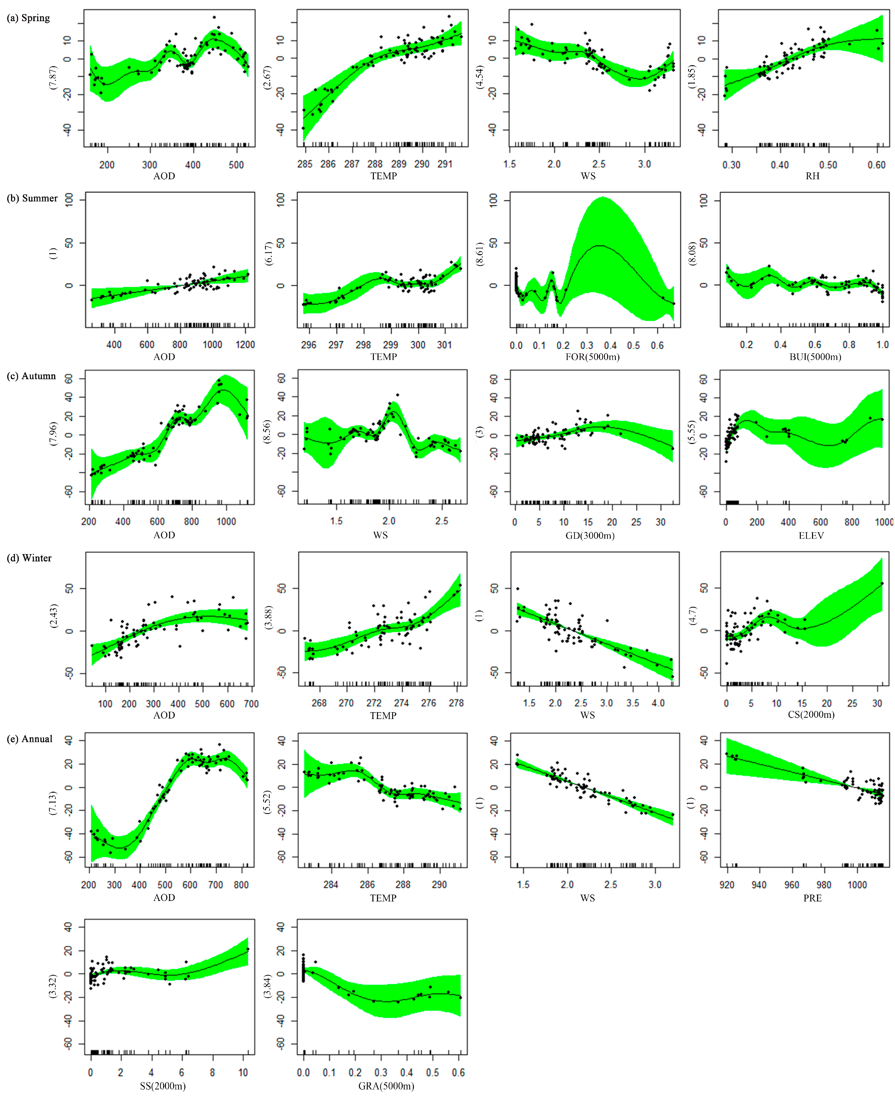
3.2. Contributing Factors of GAM Models

Figure 3 shows the individual smoothed curves for each predictor variable in GAM models. Note that a straight fitted line, corresponding to nearly one degree of freedom in Figure 3, suggests the predictor variable is fitted with a parametric linear term rather than a smoothed term. For all others, the shape of smoothed curves describes the non-linear nature of the relationships. Clearly, there are intertwined relationships between PM_2.5 concentrations and associated influencing factors. These relationships vary among predictors, as the different response curves illustrate.

Moreover, comparison of the response curves for a certain predictor across seasons and those across the entire study period further demonstrates that the contribution of a factor to PM_2.5 concentrations is not stable. This is especially clear for predictors such as AOD and wind speed. In summer and winter, AOD’s increase linearly contributes the increasing PM_2.5 concentrations, but this relationship changed to undulating non-linear ones in other periods. Among the meteorological parameters, effects of wind speed on PM_2.5 concentrations seem to vary with seasons. The PM_2.5 concentrations decreases linearly with the increase of wind speed in winter and the entire study period, and clear non-linear relationships can be observed in spring and autumn, especially the obvious wave changes in autumn.

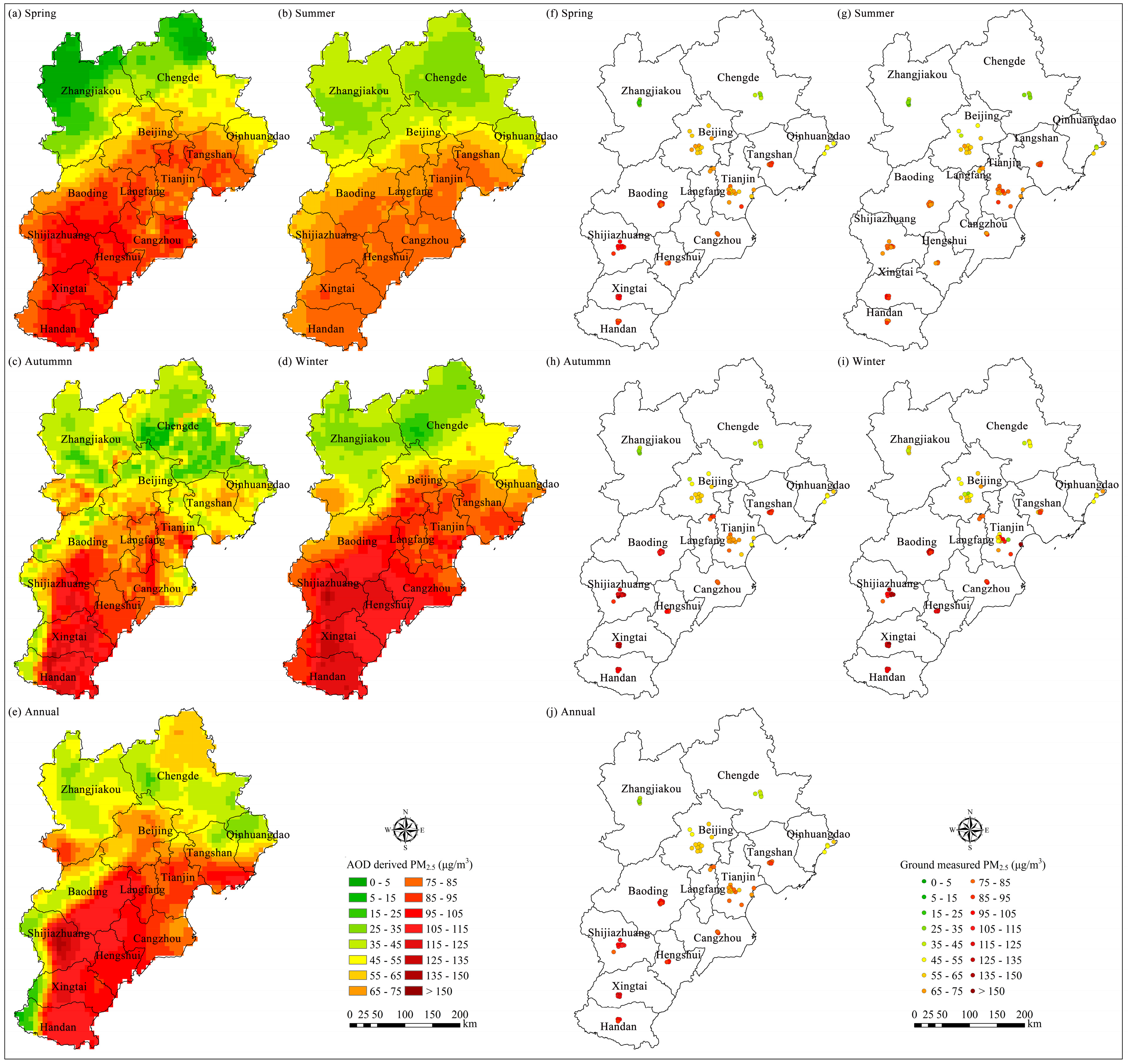
3.3. PM_2.5 Concentration Surfacesacross Time Scales

Figure 4 shows the seasonal mean and annual mean spatial patterns of the estimated PM_2.5 concentrations at a resolution of 10 km during the study period in the BTH region. To examine the spatial and seasonal prediction accuracy of the GAM model, the ground PM_2.5 measurements are also shown in Figure 4.

Clearly, the temporal and spatial patterns of AOD-derived PM_2.5 concentrations are very similar to ground measurements. Overall, the spatial patterns of the annual and seasonal mean predicted PM_2.5 concentrations are similar, with a significant north-to-south increasing gradient, and these continuous PM_2.5 concentration surfaces clearly reveal more detailed information than the stationary monitoring sites.

Spatially, higher concentrations of simulated PM_2.5 (>75 µg/m³) normally occurred in the eastern plain areas beside the Taihang Mountains, especially the internal cities of Baoding, Shijiazhuang, Xingtai, and Handan. However, the west and north parts of the Taihang Mountains have lower PM_2.5 concentrations in comparison with the plain area. Strong seasonality of PM_2.5 concentrations can also be found from the PM_2.5 concentration surfaces. Winter is the most polluted season with a mean predicted concentration of 73.8 µg/m³, while summer is the cleanest season with a mean predicted concentration of 57.5 µg/m³. The mean predicted PM_2.5 concentration is 64.2 µg/m³ in spring and 60.7 µg/m³ in autumn. The annual mean PM_2.5 estimates during the one-year study period is 69.4 µg/m³ with values varying from 13.3 µg/m³ to 133.7 µg/m³ among stations, which is almost two times higher than the level 2 value of CNAAQS and the World Health Organization Air Quality Interim Target-1 (WHO IT-1) standard of 35 µg/m³ [43].

4. Discussion

Due to the sparse distribution of stationary monitoring sites, satellite data with wide spatial coverage is growing as one of the most important supplementary tools to estimate PM_2.5 concentrations in a greater geographical space. In this process, related factors, such as meteorological parameters and pollution sources, are almost linearly integrated into the typical LUR modeling, despite the fact that the linear influencing mechanism on PM_2.5 concentration is not always suitable for all contributing factors. For this, this study develops a GAM method for satellite-based PM_2.5 concentration mapping and evaluates its temporal sensitivity by simultaneously considering the linear and non-linear relationships between PM_2.5 variation and the contributing factors.

As expected, GAM models clearly show better performance in estimating PM_2.5 concentrations with satellite based AOD compared with the benchmark LUR models in the BTH region. The CV R² (i.e., 0.90) and RMSE (i.e., 7.52 μg/m³) at the annual scale are even better than any previously reported ones (i.e., CV R² = 0.87 and RMSE = 19.2 μg/m³) in LUR modeling [44]. This result definitely confirms the necessity of GAM modeling in simultaneously involving the linear and non-linear hypothesis between PM_2.5 variation and associated factors in the accurate estimation of PM_2.5 concentrations. Moreover, the difference of the finally determined predictor variables of GAM models and LUR models suggests that satellite-based PM_2.5 estimation can be achieved using a nonlinear statistical technique with highly attributable factors rather than those simply identified with linearly empirical-statistical modeling.

Meanwhile, results in Table 2 also reveal that predictor variables in the final GAM models of this study differ markedly by season except for the AOD. Overall, the relationship between AOD and PM_2.5 is always positive and consistent for all of the GAM models across seasonal and annual scales, sometimes even with nonlinear undulations. Nevertheless, this relationship varies significantly with regions over time because the aerosol chemical components and the optical properties are spatially and temporally inhomogeneous. This finding actually confirms, again, the feasibility and fair stability of GAM modeling in satellite-based estimation of PM_2.5 concentration. However, the contribution of auxiliary factors varies much in this process due to the influence of the complex interactions between meteorological conditions and pollution sources. For example, PM_2.5 concentrations tended to decrease in spring, autumn, and winter with the higher wind speeds in terms of the acceleration of atmospheric dilution and diffusion in this study, but the wind speed is not a factor that significantly influences the PM_2.5 variations in summer. Therefore, it is necessary to detect the real attributable factors impacting PM_2.5 variations at different periods of time when initiating policies to reduce PM_2.5 pollution.

Overall, most associations between the selected predictors and PM_2.5 concentrations illustrated in Figure 3 are within our expectation. For meteorological parameters, higher wind speeds tend to decrease PM_2.5 concentrations, on account of the atmospheric dilution and diffusion process. Higher temperatures are associated with higher PM_2.5 concentrations, which accelerate the production of secondary aerosols, and also evaporate ammonium nitrate and organic aerosols to some extent. Relative humidity is positively correlated with PM_2.5 concentration, possibly because water drops absorb PM_2.5 at high humidity, which may aggravates the accumulation of particulate matter at the same time. Higher pressure is usually associated with greater concentrations. This can be explained by the fact that it is associated with stable air conditions, which decrease the pollutant dispersion to some extent. To our knowledge, lower wind speed, together with higher temperatures and humidity, is usually accompanied with temperature inversion or foggy weather in spring and winter, which is beneficial to an atmospheric surface layer to maintain a stable state and, therefore, hindered the diffusion of PM_2.5 in both vertical and horizontal directions, as well as facilitates the formation of secondary particles. Land use predictors, such as grasslands, would decrease PM_2.5 concentration probably owning to the adsorption and retardation capacity of vegetation, which also protects the surface soil and prevent the surface dust. However, built-up area and forests area follow nonlinear undulating patterns in relation to PM_2.5 concentration and we have found no obvious reason for this. As a result, differential dynamic effects of the impacting factors of PM_2.5 at different periods should be taken into consideration when initiating policies to reduce PM_2.5 pollution in China. This study also verifies that investigating the effects of impacting factors of PM_2.5 concentration using nonparametric additive regression models is reasonable and applicable.

Compared with previous studies with limited data accessibility, this study might be the first one with refined industrial polluting sources and ground dust surfaces for PM_2.5 concentration estimation. With these refined data input, we clearly find that industrial plants and ground dust are the two most important contributing sources to the variations of PM_2.5 concentrations in the BTH region through GAM modeling. The number of industrial plants may better reflect the industrial land use and industry intensity. The contribution of ground dust to PM_2.5 is also significant, which is identified as one of the major sources of PM_2.5 in this region. These results indicate that specific pollution sources are helpful for improving the satellite-based empirical-statistical modeling of PM_2.5 concentrations. They actually also suggest that satellite-based GAM modeling could potentially depict the real pollution sources, which cause the variation of PM_2.5 concentration, by considering the influencing mechanism through the non-linear hypothesis of the relationship between PM_2.5 concentrations and influencing factors.

With the robust GAM models developed in this study, the seasonal and annual spatial distribution of PM_2.5 concentrations in the BTH region is successfully plotted. While the monitoring site-based accuracy of these figures are theoretically higher than those previously reported [9]. The spatial heterogeneity of PM_2.5 concentrations illustrated in Figure 4 actually implies the defect of GAM modeling. Similar to LUR modeling, the coefficient of each predictor variable in a GAM model is spatially consistent, but this does violate the fact that the impact of an attributable factor on the PM_2.5 concentration variation is generally spatially dependent. This might be the reason of the too smoothed effects of PM_2.5 concentrations in Figure 4, such as the area of Shijiazhuang city. In this way, further work can focus on the improvement of the GAM modeling in depicting the spatial distributions of PM_2.5 concentrations with a fine spatial resolution. It is possible to implement this work by introducing the satellite-based AODs at 3 km or 1 km scales. Additionally, considering the specific advantages of the non-linear hypothesis in simulating the instant variation of PM_2.5 concentration, GAM models in the future could be developed on a short-term scale, such as daily or even hourly scales. In this process, a full space–time model would be needed to better demonstrate the spatial-temporal variation of PM_2.5 concentrations as GAMs are unable to differentiate spatial heterogeneity of factors contributing to changing PM_2.5 over time, which might lead to the residual spatial autocorrelation.

5. Conclusions

Aiming to modify the unreasonable linear hypothesis of current satellite-based methods for PM_2.5 concentration estimation, GAM models considering the linear and non-linear relationships between PM_2.5 variation and associated contributing factors were proposed in this study. In the case of the BTH region, China, GAM models at both the seasonal and annual scales clearly outperformed typical LUR models in simulating PM_2.5 concentrations, with the CV R² values of 0.92, 0.78, 0.87, 0.85, and 0.90, respectively, and RMSEs at 6.23, 8.91, 10.49, 14.05, and 7.52 μg/m³, respectively. The spatial variations and seasonal variations of PM_2.5 concentrations in the BTH region can also be depicted by GAM models. Results of this study highlight that GAM modeling is a robust method for satellite-based estimation of PM_2.5 concentrations using the adaptively integrated linear and non-linear statistical modeling techniques. With the capacity of fusing spatial heterogeneity of attributable factors, GAM modeling could be a promising way for fine spatial-temporal scale mapping of PM_2.5 concentrations in the coming future and consequently promotes the widespread applications of remote sensing in air pollution mapping.

References

1. Pope, C.A., III; Dockery, D.W. Health effects of fine particulate air pollution: Lines that connect. J. Air Waste Manag. 2006, 56, 709–742. [Google Scholar] [CrossRef]
2. Sacks, J.D.; Stanek, L.W.; Luben, T.J.; Johns, D.O.; Buckley, B.J.; Brown, J.S.; Ross, M. Particulate matter-induced health effects: Who is susceptible? Environ. Health Perspect. 2011, 119, 446–454. [Google Scholar] [CrossRef] [PubMed]
3. Crouse, D.L.; Peters, P.A.; van Donkelaar, A.; Goldberg, M.S.; Villeneuve, P.J.; Brion, O.; Khan, S.; Atari, D.O.; Jerrett, M.; Pope, C.A., III; et al. Risk of nonaccidental and cardiovascular mortality in relation to long-term exposure to low concentrations of fine particulate matter: A Canadian national-level cohort study. Environ. Health Perspect. 2012, 120, 708. [Google Scholar] [CrossRef] [PubMed]
4. Zou, B.; Wilson, J.G.; Zhan, F.B.; Zeng, Y. Air pollution exposure assessment methods utilized in epidemiological studies. J. Environ. Monit. 2009, 11, 475–490. [Google Scholar] [CrossRef] [PubMed]
5. Lim, S.S.; Vos, T.; Flaxman, A.D.; Danaei, G.; Shibuya, K.; Adair-Rohani, H.; AlMazroa, M.A.; Amann, M.; Anderson, H.R.; Andrews, K.G.; et al. A comparative risk assessment of burden of disease and injury attributable to 67 risk factors and risk factor clusters in 21 regions, 1990–2010: A systematic analysis for the Global Burden of Disease Study 2010. Lancet 2013, 380, 2224–2260. [Google Scholar] [CrossRef]
6. Boys, B.L.; Martin, R.V.; van Donkelaar, A.; MacDonell, R.J.; Hsu, N.C.; Cooper, M.J.; Yantosca, R.M.; Lu, Z.; Streets, D.G.; Zhang, Q.; et al. Fifteen-year global time series of satellite-derived fine particulate matter. Environ. Sci. Technol. 2014, 48, 11109–11118. [Google Scholar] [CrossRef] [PubMed]
7. Van Donkelaar, A.; Martin, R.V.; Brauer, M.; Kahn, R.; Levy, R.; Verduzco, C.; Villeneuve, P.J. Global estimates of ambient fine particulate matter concentrations from satellite-based aerosol optical depth: Development and application. Environ. Health Perspect. 2010, 118, 847–855. [Google Scholar] [CrossRef] [PubMed]
8. Li, C.; Hsu, N.C.; Tsay, S.C. A study on the potential applications of satellite data in air quality monitoring and forecasting. Atmos. Environ. 2011, 45, 3663–3675. [Google Scholar] [CrossRef]
9. Zou, B.; Pu, Q.; Bilal, M.; Weng, Q.; Zhai, L.; Nichol, J.E. High-resolution satellite mapping of fine particulates based on geographically weighted regression. IEEE Trans. Geosci. Remote Sens. 2016, 13, 495–499. [Google Scholar] [CrossRef]
10. Song, W.; Jia, H.; Huang, J.; Zhang, Y. A satellite-based geographically weighted regression model for regional PM2.5 estimation over the Pearl River Delta region in China. Remote Sens. Environ. 2014, 154, 1–7. [Google Scholar] [CrossRef]
11. Liu, Y.; Paciorek, C.J.; Koutrakis, P. Estimating regional spatial and temporal variability of PM2.5 concentrations using satellite data, meteorology, and land use information. Environ. Health Perspect. 2009, 117, 886–892. [Google Scholar] [CrossRef] [PubMed] [Green Version]
12. Ma, Z.; Hu, X.; Huang, L.; Bi, J.; Liu, Y. Estimating ground-level PM2.5 in China using satellite remote sensing. Environ. Sci. Technol. 2014, 48, 7436–7444. [Google Scholar] [CrossRef] [PubMed]
13. Zou, B.; Zhan, F.B.; Wilson, J.G.; Zeng, Y. Performance of AERMOD at different time scales. Simul. Model. Pract. Theory 2010, 18, 612–623. [Google Scholar] [CrossRef]
14. Jowett, I.G.; Parkyn, S.M.; Richardson, J. Habitat characteristics of crayfish (Paranephrops planifrons) in New Zealand streams using generalised additive models (GAMs). Hydrobiologia 2008, 596, 353–365. [Google Scholar] [CrossRef]
15. Leathwick, J.R.; Elith, J.; Hastie, T. Comparative performance of generalized additive models and multivariate adaptive regression splines for statistical modelling of species distributions. Ecol. Model. 2006, 199, 188–196. [Google Scholar] [CrossRef]
16. Chen, C.C.; Wu, C.F.; Yu, H.L.; Chan, C.-C.; Cheng, T.S. Spatiotemporal modeling with temporal-invariant variogram subgroups to estimate fine particulate matter PM2.5 concentrations. Atmos. Environ. 2012, 54, 1–8. [Google Scholar] [CrossRef]
17. Li, L.; Wu, J.; Ghosh, J.K.; Ritz, B. Estimating spatiotemporal variability of ambient air pollutant concentrations with a hierarchical model. Atmos. Environ. 2013, 71, 54–63. [Google Scholar] [CrossRef] [PubMed]
18. Ma, Z.W.; Hu, X.F.; Sayer, A.M.; Levy, R.; Zhang, Q.; Xue, Y.G.; Tong, S.L.; Bi, J.; Huang, L.; Liu, Y. Satellite-based spatiotemporal trends in PM2.5 concentrations: China, 2004–2013. Environ. Health Perspect. 2015. [Google Scholar] [CrossRef] [PubMed]
19. Xu, P.; Chen, Y.; Ye, X. Haze, air pollution, and health in China. Lancet 2013, 382, 2067. [Google Scholar] [CrossRef]
20. Chang, Y. China needs a tighter PM2.5 limit and a change in priorities. Environ. Sci. Technol. 2012, 46, 7069–7070. [Google Scholar] [CrossRef] [PubMed]
21. Gao, M.; Guttikunda, S.K.; Carmichael, G.R.; Wang, Y.; Liu, Z.; Stanier, C.O.; Saide, P.E.; Yu, M. Health impacts and economic losses assessment of the 2013 severe haze event in Beijing area. Sci. Total Environ. 2015, 511, 553–561. [Google Scholar] [CrossRef] [PubMed]
22. Dan, M.; Zhuang, G.; Li, X.; Tao, H.; Zhuang, Y. The characteristics of carbonaceous species and their sources in PM2.5 in Beijing. Atmos. Environ. 2004, 38, 3443–3452. [Google Scholar] [CrossRef]
23. Zheng, M.; Salmon, L.G.; Schauer, J.J.; Zeng, L.; Kiang, C.S.; Zhang, Y.; Cass, G.R. Seasonal trends in PM2.5 source contributions in Beijing, China. Atmos. Environ. 2005, 39, 3967–3976. [Google Scholar] [CrossRef]
24. Che, H.; Xia, X.; Zhu, J.; Li, Z.; Dubovik, O.; Holben, B.; Goloub, P.; Chen, H.; Estelles, V.; Cuevas-Agulló, E.; et al. Column aerosol optical properties and aerosol radiative forcing during a serious haze-fog month over North China Plain in 2013 based on ground-based sunphotometer measurements. Atmos. Chem. Phys. 2014, 14, 2125–2138. [Google Scholar] [CrossRef] [Green Version]
25. Guo, S.; Hu, M.; Zamora, M.L.; Peng, J.; Shang, D.; Zheng, J.; Du, Z.; Wu, Z.; Shao, M.; Zeng, L.; et al. Elucidating severe urban haze formation in China. Proc. Natl. Acad. Sci. USA 2014, 111, 17373–17378. [Google Scholar] [CrossRef] [PubMed]
26. Meng, X.; Chen, L.; Cai, J.; Zou, B.; Wu, C.F.; Fu, Q.; Zhang, Y.; Liu, Y.; Kan, H. A land use regression model for estimating the NO2 concentration in shanghai, China. Environ. Res. 2015, 137, 308–315. [Google Scholar] [CrossRef] [PubMed]
27. Fang, X.; Zou, B.; Liu, X.; Sternberg, T.; Zhai, L. Satellite-based ground PM2.5 estimation using timely structure adaptive modeling. Remote Sens. Environ. 2016, 186, 152–163. [Google Scholar] [CrossRef]
28. Remer, L.A.; Kaufman, Y.J.; Tanré, D.; Mattoo, S.; Chu, D.A.; Martins, J.V.; Li, R.-R.; Ichoku, C.; Levy, R.C.; Kleidman, R.G.; et al. The MODIS aerosol algorithm, products, and validation. J. Atmos. Sci. 2005, 62, 947–973. [Google Scholar] [CrossRef]
29. Levy, R.C.; Remer, L.A.; Mattoo, S.; Vermote, E.F.; Kaufman, Y.J. Second-generation operational algorithm: Retrieval of aerosol properties over land from inversion of Moderate Resolution Imaging Spectroradiometer spectral reflectance. J. Geophys. Res. Atmos. 2007, 112. [Google Scholar] [CrossRef]
30. Levy, R.C.; Remer, L.A.; Tanré, D.; Mattoo, S.; Kaufman, Y.J. Algorithm for Remote Sensing of Tropospheric Aerosol over Dark Targets from MODIS: Collections 005 and 051: Revision 2; 2009. Available online: http://modisatmos.gsfc.nasa.gov/_docs/ATBD_MOD04_C005_rev2.pdf (accessed on 9 January 2016).
31. Levy, R.C.; Remer, L.A.; Kleidman, R.G.; Mattoo, S.; Ichoku, C.; Kahn, R.; Eck, T.F. Global evaluation of the Collection 5 MODIS dark-target aerosol products over land. Atmos. Chem. Phys. 2010, 10, 10399–10420. [Google Scholar] [CrossRef] [Green Version]
32. Lee, H.J.; Liu, Y.; Coull, B.A.; Schwartz, J.; Koutrakis, P. A novel calibration approach of MODIS AOD data to predict PM2.5 concentrations. Atmos. Chem. Phys. 2011, 11, 7991–8002. [Google Scholar] [CrossRef]
33. Liu, Y.; Franklin, M.; Kahn, R.; Koutrakis, P. Using aerosol optical thickness to predict ground-level PM2.5 concentrations in the St. Louis area: A comparison between MISR and MODIS. Remote Sens. Environ. 2007, 107, 33–44. [Google Scholar] [CrossRef]
34. Tian, J.; Chen, D. A semi-empirical model for predicting hourly ground-level fine particulate matter (PM2.5) concentration in southern Ontario from satellite remote sensing and ground-based meteorological measurements. Remote Sens. Environ. 2010, 114, 221–229. [Google Scholar] [CrossRef]
35. Zou, B.; Peng, F.; Wan, N.; Wilson, J.G.; Xiong, Y. Sulfur dioxide exposure and environmental justice: A multi-scale and source-specific perspective. Atmos. Pollut. Res. 2014, 5, 491–499. [Google Scholar] [CrossRef]
36. Zou, B.; Luo, Y.; Wan, N.; Zheng, Z.; Sternberg, T.; Liao, Y. Performance comparison of LUR and OK in PM2.5 concentration mapping: A multidimensional perspective. Sci. Rep. 2015, 5, 8698. [Google Scholar] [CrossRef] [PubMed]
37. Hastie, T.J.; Tibshirani, R.J. Generalized additive models. Stat. Sci. 1986, 1, 297–310. [Google Scholar] [CrossRef]
38. Duchon, J. Splines Minimizing Rotation-Invariant Semi-Norms in Sobolev Spaces. In Constructive Theory of Functions of Several Variables; Springer: Berlin/Heidelberg, Germany, 1977; pp. 85–100. [Google Scholar]
39. Wood, S.N. Thin plate regression splines. J. R. Stat. Soc. Ser. B 2003, 65, 95–114. [Google Scholar] [CrossRef]
40. Wood, S.N. MGCV: GAMs and generalized ridge regression for R. R News 2001, 1, 20–25. [Google Scholar]
41. Chambers, J.M.; Hastie, T.J. Statistical Models in S; CRC Press, Inc.: Boca Raton, FL, USA, 1991. [Google Scholar]
42. Rodriguez, J.D.; Perez, A.; Lozano, J.A. Sensitivity analysis of k-fold cross validation in prediction error estimation. IEEE Trans. Pattern Anal. Mach. Intell. 2010, 32, 569–575. [Google Scholar] [CrossRef] [PubMed]
43. Chinese National Ambient Air Quality Standards, GB 3095-2012. Available online: http://kjs.mep.gov.cn/hjbhbz/bzwb/dqhjbh/dqhjzlbz/201203/t20120302_224165.htm (accessed on 12 January 2016).
44. Meng, X.; Fu, Q.; Ma, Z.; Chen, L.; Zou, B.; Zhang, Y.; Xue, W.; Wang, J.; Wang, D.; Kan, H.; Liu, Y. Estimating ground-level PM10 in a Chinese city by combining satellite data, meteorological information and a land use regression model. Environ. Pollut. 2016, 208, 177–184. [Google Scholar] [CrossRef] [PubMed]
Figure 1. Sketch map of the Beijing-Tianjin-Hebei (BTH) region in this study.
Remotesensing 09 00001 g001
Figure 2. Scatterplots of GAM model fitting and validating results. The dashed line is the 1:1 line as a reference. (ae) are GAM model fitting results of spring, summer, autumn, winter, and annual, respectively; (fj) are 10-fold validating results for GAM model of spring, summer, autumn, winter, and annual, respectively.
Remotesensing 09 00001 g002
Figure 3. Partial response plots of PM2.5 predictors. The individual smoothed curve for each predictor variable is shown as solid lines, with 95% confidence limits shown as shaded areas. The x-axis represents the frequency of data; the y-axis represents the marginal effects. Estimated degrees of freedom for each smooth term are given as the number in y-axis caption. (ae) are partial response plots for GAM model of spring, summer, autumn, winter, and annual, respectively. AOD = aerosol optical depth; WS = wind speed; TEMP = temperature; RH = relative humidity; PRE = atmospheric pressure; GD = percentage of all ground dust area; CS = percentage of construction site area; SS = percentage of stacked substance area; BUI = percentage of built-up area; FOR = percentage of forests area; GRA = percentage of grasslands area; ELEV = elevation; and PM = number of papermaking plants.
Remotesensing 09 00001 g003
Figure 4. Comparisons of seasonal and annual mean AOD-derived PM2.5 and ground-measured PM2.5 concentrations. (ae) are AOD-derived PM2.5 concentrations of spring, summer, autumn, winter, and annual, respectively; (fj) are ground-measured PM2.5 concentrations of spring, summer, autumn, winter, and annual, respectively.
Remotesensing 09 00001 g004