Automated Reconstruction of Building LoDs from Airborne LiDAR Point Clouds Using an Improved Morphological Scale Space

Abstract

Reconstructing building models at different levels of detail (LoDs) from airborne laser scanning point clouds is urgently needed for wide application as this method can balance between the user’s requirements and economic costs. The previous methods reconstruct building LoDs from the finest 3D building models rather than from point clouds, resulting in heavy costs and inflexible adaptivity. The scale space is a sound theory for multi-scale representation of an object from a coarser level to a finer level. Therefore, this paper proposes a novel method to reconstruct buildings at different LoDs from airborne Light Detection and Ranging (LiDAR) point clouds based on an improved morphological scale space. The proposed method first extracts building candidate regions following the separation of ground and non-ground points. For each building candidate region, the proposed method generates a scale space by iteratively using the improved morphological reconstruction with the increase of scale, and constructs the corresponding topological relationship graphs (TRGs) across scales. Secondly, the proposed method robustly extracts building points by using features based on the TRG. Finally, the proposed method reconstructs each building at different LoDs according to the TRG. The experiments demonstrate that the proposed method robustly extracts the buildings with details (e.g., door eaves and roof furniture) and illustrate good performance in distinguishing buildings from vegetation or other objects, while automatically reconstructing building LoDs from the finest building points.

1. Introduction

Three-dimensional (3D) building models play an important role in urban planning and management, telecommunications, tourism, disaster relief and evaluation, environmental simulation, vehicle navigation, and so on [1]. Automatically reconstructing building models at different levels of detail (LoDs) is important for various applications. For example, the finest model would be taken as the basis for assessing solar potential of rooftops [2], and a coarser model could satisfy personal navigation in a mobile device [3].

The LoDs of buildings are the multiple representations of 3D building models. In the past decade, many researchers have concentrated on the generation of LoDs from the finest 3D building models [4,5,6,7,8]. Generally, most methods derive coarse LoD models by employing the operators of simplification and aggregation on a fine-scale 3D building model [5,7] or on the 2D ground plans [4,6,9]. However, there are many definitions for LoDs, and the standard is still not unified [4,10]. After the CityGML (OGC City Geography Markup Language) standard was published [1], many studies focused on deriving coarse models from a fine-scale 3D model according to the framework of CityGML. Mao et al. generated CityGML models by simplification and aggregation, and then transformed the generated CityGML models to a CityTree for realizing dynamic zoom functionality in real time [6]. Fan and Meng proposed a three-step approach to simplify and aggregate 2D ground plans and generalize roof structures [4]. Verdie et al. generated building LoDs from the finest LoD to the coarsest LoD based on surface meshes [11]. In a word, the above-reported methods generate 3D building models at different LoDs from a fine-scale building model. However, reconstructing a fine-scale building model is quite expensive and may not be relevant for many applications. Moreover, the number of levels for discrete LoDs is fixed and thus limited in the framework of CityGML, and the large difference between two adjacent building LoDs could cause a big jump from one level to another level in the visualization [3,10]. Hence, automatically reconstructing a 3D building model at desired levels from 3D information of buildings rather than from a fine-scale 3D building model is an economical and flexible way to meet the user’s requirements.

Airborne Light Detection and Ranging (LiDAR) has become a mature technology for capturing 3D information of buildings [12], which could be taken as the basis for generating building LoDs. At present, robustly extracting building points from various and complex urban scenes is still a challenging issue [13,14]. In the last decade, numerous methods have been reported for extracting building information from airborne laser scanning points, including DSM (Digital Surface Model)-based methods [15], point cloud-based methods [16] and methods based on imagery-fusing point clouds [17]. With the improvement of point density and the penetrating capacity of commercial LiDAR systems (e.g., Full Waveform LiDAR systems), the point cloud-based methods could be more suitable for complicated urban scenes. In general, segmentation-based methods and supervised learning-based methods are two main solutions for building extraction based on point clouds. Supervised learning-based methods [18,19,20,21,22,23] first select some building and non-building data as samples for training classifiers, and then extract building points. However, it is time consuming in selecting samples, and the result is highly dependent on samples [14]. Segmentation-based methods begin by splitting point clouds into disjointed segments, and then extract building segments with some prior knowledge or assumptions [16,24,25,26,27]. Generally, segmentation-based methods are widely utilized in various engineering applications. These methods take each segment as an individual unit, although many features derived from a single local segment cannot describe the differences between buildings and other objects properly, causing classification errors. Fortunately, it can perform better when the method combines features derived from the entire object with features derived from the local neighbors, just like the human visual system distinguishes different objects from the whole to the local [28]. The key step is to link the relationship between the segments of a building and the entire building, and it is of great importance to generate building LoDs from extracted segments.

Scale-space theory lays a sound foundation for representing one object from a finer level to a coarser level [29]. It gradually ignores the details and merges parts of an object into a group with the increasing of the scale and could directly generate an arbitrary level from the finest point clouds when the corresponding scale is given. Moreover, it maintains the spatial relations between adjacent scales, and provides a good way to imitate the human visual system (HVS) for perceiving objects ranging from whole to local details [28]. Generally, scale spaces can be constructed by wavelet transform [30], Gaussian smoothing [31], and mathematical morphology [32]. The scale space constructed by mathematical morphology is non-linear, and it is good for maintaining the shape of an object. It has been widely used in various fields, such as signal processing and image processing [29]. Vu et al. generated a DSM from airborne laser scanning point clouds and constructed the scale space with area morphology for building extraction by fusing spectral imageries, and providing the simple models with multi-scale representation [33]. Nevertheless, loss of information (e.g., the multiple returns) in the generation of DSMs affect the extraction of buildings, and the method ignores the local details (e.g., dormers and other roof elements) of the building model in the multi-scale representation. Fortunately, the scale space constructed by the morphological reconstruction (e.g., opening and closing by reconstruction) generates the LoDs of an object by controlling the scale (e.g., the size of a structuring element in morphology). It could better describe the local changes of objects across different levels by the smoothing operators of opening and closing [32]. Hence, we propose a novel method to extract building points and generate 3D building LoDs from airborne LiDAR point clouds by applying the morphological scale space, where each level is directly generated from point clouds by the morphological reconstruction. The main contributions of the proposed method are as follows.

• Directly construct the scale space from airborne laser scanning point clouds by applying the morphological reconstruction with planar segment constraints for feature preservation, and a TRG (topological relationship graph) is created for representing the spatial relations between segments across levels;
• Generate 3D building LoDs from the extracted building points based on the TRG, and the building LoD with a specified level could be automatically reconstructed from the finest building points.

The remainder of this paper is organized as follows. An improved morphological scale-space for point clouds is elaborated in Section 2. Section 3 describes the generation of building LoDs from airborne laser scanning point clouds based on the improved morphological scale space. In Section 4, the experimental studies that were undertaken to evaluate the proposed method are outlined. Finally, conclusions are drawn at end of this paper.

2. An Improved Morphological Scale Space for Point Clouds

The improved morphological scale space is iteratively constructed by a morphological reconstruction with planar segment constraints with the increasing of scale. Moreover, the topological relationship graph (TRG) describing the spatial relations between different levels of one object is generated for extracting building points and reconstructing 3D building LoDs.

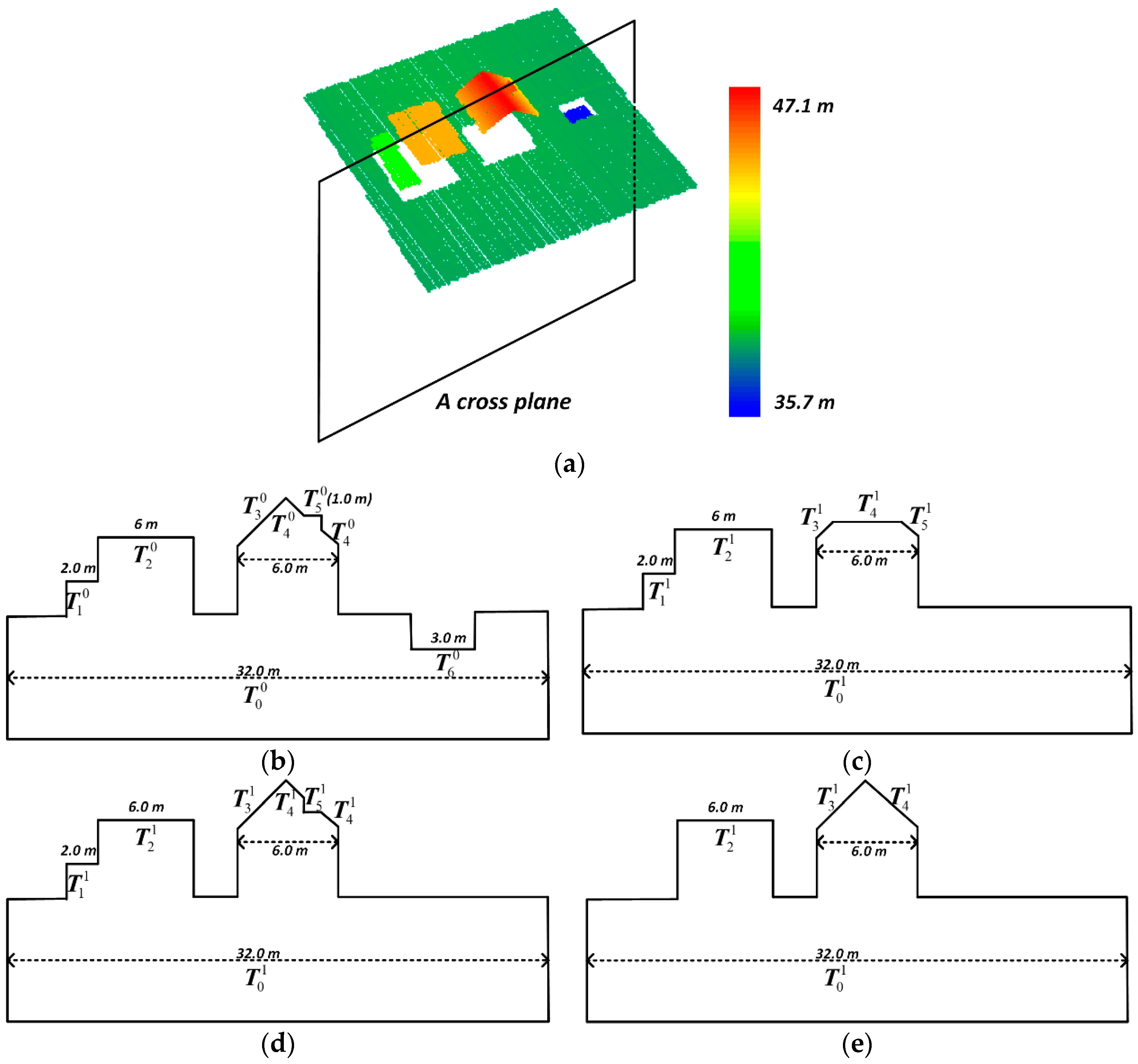
2.1. A Morphological Reconstruction for Each Level with Planar Segment Constraints

The improved morphological reconstruction on the point clouds includes two steps, the opening by reconstruction and the closing by reconstruction. Although the exterior shape of an object could be maintained, part of an inclined roof may be flattened during the morphological reconstruction. It leads to a failure in linking the topology between different levels. To overcome the drawback, the result of a plane segmentation is adopted as constraints. The improved morphological reconstruction is described as follows.

Let P = {p₀, p₁,…, p_n} be the point clouds. $P$ is segmented by the plane segmentation method of [34] and small segments are removed by the threshold $t_N$, which is defined as the number of points in one segment. The remained segments are denoted as PS = {PS₀, PS₁, PS₂,…}, and all points in the removed segments are pushed into one set of individual points. Moreover, the slope of each segment is calculated, and each segment is robustly labeled as horizontal or inclined by Equation (1) to avoid the disturbance of noises.

$$L_{p{s}_i}=\{\begin{array}{cc}1& if{S}_{p{s}_i}\ge t_S\\ 0& if{S}_{p{s}_i}<t_S\end{array}$$

(1)

where $S_{p{s}_i}$ is the slope of the segment $p{s}_i$; $t_S$ is the slope threshold; $L_{p{s}_i}$ is assigned to 1 or 0 for marking one segment to be horizontal or inclined.

Then, the opening reconstruction operator is defined as follows: Set an arbitrary value $s$ as the current scale, which is taken as the radius of a window $B_s$, and perform an opening operator on point clouds $P$ according to Equation (2) to flatten the sharp details, which are smaller than two times $s$, and the result is denoted as $P_{OPEN}$. $P_{OPEN}$ is taken as the marker point clouds, and $P$ is the mask point clouds. A geodesic dilation with a window $B_I$ is adopted iteratively according to Equations (3) and (4) until the result is stable [32]. The result of the opening by reconstruction is denoted as $P_{OPEN\_REC}={\delta }_P^{\left(n\right)}\left(P_{OPEN}\right)$.

$$P_{OPEN}=\left(P\ominus B_s\right)\oplus B_s$$

(2)

$${\delta }_P^{\left(1\right)}\left(P_{OPEN}\right)=\left(P_{OPEN}\oplus B_I\right)\wedge P$$

(3)

$${\delta }_P^{\left(n\right)}\left(P_{OPEN}\right)={\delta }_P^{\left(1\right)}\circ {\delta }_P^{\left(1\right)}\circ \dots \circ {\delta }_P^{\left(1\right)}\left(P_{OPEN}\right)$$

(4)

where $\oplus$ is the operator of the dilation; $\ominus$ is the operator of the erosion; $\delta$ is the operator of the geodesic dilation; $\wedge$ stands for the point-wise minimum; $n$ is the iteration number.

The closing reconstruction operator is defined as follows: Perform a closing operator with the disc window ($B_s$) on $P_{OPEN\_REC}$ according to Equation (5) to remove lower details, which are smaller than two times $s$, and the result is denoted as $P_{CLOSE}$. $P_{CLOSE}$ is taken as the marker point clouds, and $P_{OPEN\_REC}$ is the mask point clouds. A geodesic erosion is adopted iteratively according to Equations (6) and (7) until the result is stable [32]. The result of the closing by reconstruction $P_{CLOSE\_REC}={\epsilon }_{P_{OPEN\_REC}}^{\left(n\right)}\left(P_{CLOSE}\right)$ is regarded as the reconstruction result at the level of $s$.

$$P_{CLOSE}=\left(P_{\mathit{OPEN}\_\mathit{REC}}\oplus B_s\right)\ominus B_s$$

(5)

$${\epsilon }_{P_{OPEN\_REC}}^{\left(1\right)}\left(P_{CLOSE}\right)=\left(P_{CLOSE}\ominus B_I\right)\vee P_{OPEN\_REC}$$

(6)

$${\epsilon }_{P_{OPEN\_REC}}^{\left(n\right)}\left(P_{CLOSE}\right)={\epsilon }_{P_{OPEN\_REC}}^{\left(1\right)}\circ {\epsilon }_{P_{OPEN\_REC}}^{\left(1\right)}\circ \dots \circ {\epsilon }_{P_{OPEN\_REC}}^{\left(1\right)}\left(P_{CLOSE}\right)$$

(7)

where $\epsilon$ is the operator of geodesic erosion, $\vee$ stands for the point-wise maximum, and $n$ is the number of iterations.

For example, one building is illustrated in Figure 1a, and Figure 1b shows a cross-section of that building. Figure 1c shows the result of the morphological reconstruction at the scale of 2 m. It shows that $T_6^0$ is flattened onto the larger segment, but $T_3^0$ and $T_4^0$ are erroneously processed as three segments ($T_3^1,T_4^{1}and{T}_5^1$). The phenomenon is the canonical cut-off problem in the morphological operator [35] and will result in a failure of relinking the relationships between these segments from adjacent levels. In order to address the problem, a segment is restricted to two states after the morphological reconstruction: one horizontal segment or itself. The result of plane segmentation ($PS$) is adopted to correct the result of morphological reconstruction. First, we design an indicator to check whether a segment becomes horizontal or not after the morphological reconstruction. If the elevation difference $h_{p{s}_i}$ as described by Equation (8) is less than a threshold $t_{SH}$, the segment is marked as horizontal in Equation (9). Otherwise, the elevations of the point in the segment are recovered by the corresponding value after the morphological reconstruction. Figure 1d is the result after the modification.

$$h_{p{s}_i}=(h_{MAX}-h_{MIN})\times L_{p{s}_i}$$

(8)

$$L_{p{s}_i}^{*}=\{\begin{array}{cc}1& if{h}_{p{s}_i}\ge t_{SH}\\ 0& if{h}_{p{s}_i}<t_{SH}\end{array}$$

(9)

where $h_{MAX}$ and $h_{MIN}$ are the maximum and minimum elevation in the segment $p{s}_i$ after morphological reconstruction; $h_{p{s}_i}$ is the indicator; $t_{SH}$ is the threshold; and $L_{p{s}_i}^{*}$ is the judged result by the indicator.

Additionally, although some segments are smaller than twice the scale, they may fail to be removed. For example, there are two small segments $T_1^1$ and $T_5^1$ in Figure 1d, which is the morphological reconstruction result at the scale of 2 m, and they fail to flatten into the segments $T_0^1$ and $T_4^1$. Therefore, the method automatically edits these false segments through two steps. The first step is that the method detects these false segments according to their size and relationship with the neighboring segments. For the first case $T_1^1$, the method first groups all segments into different clusters according to adjacent segments with a minor elevation difference in the vertical direction, and each cluster is taken as an individual structure. Then, segments of any cluster which is smaller than two times the scale are detected. For the second case $T_5^1$, the method checks each small segment with a width less than twice the scale. If a small segment is included in another segment which is larger than two times the scale, the small segment will be detected. After detection of false segments, the method searches a neighboring segment with the width larger than twice the scale to modify each false segment. Figure 1e is the final result of the improved morphological reconstruction at the scale of 2 m.

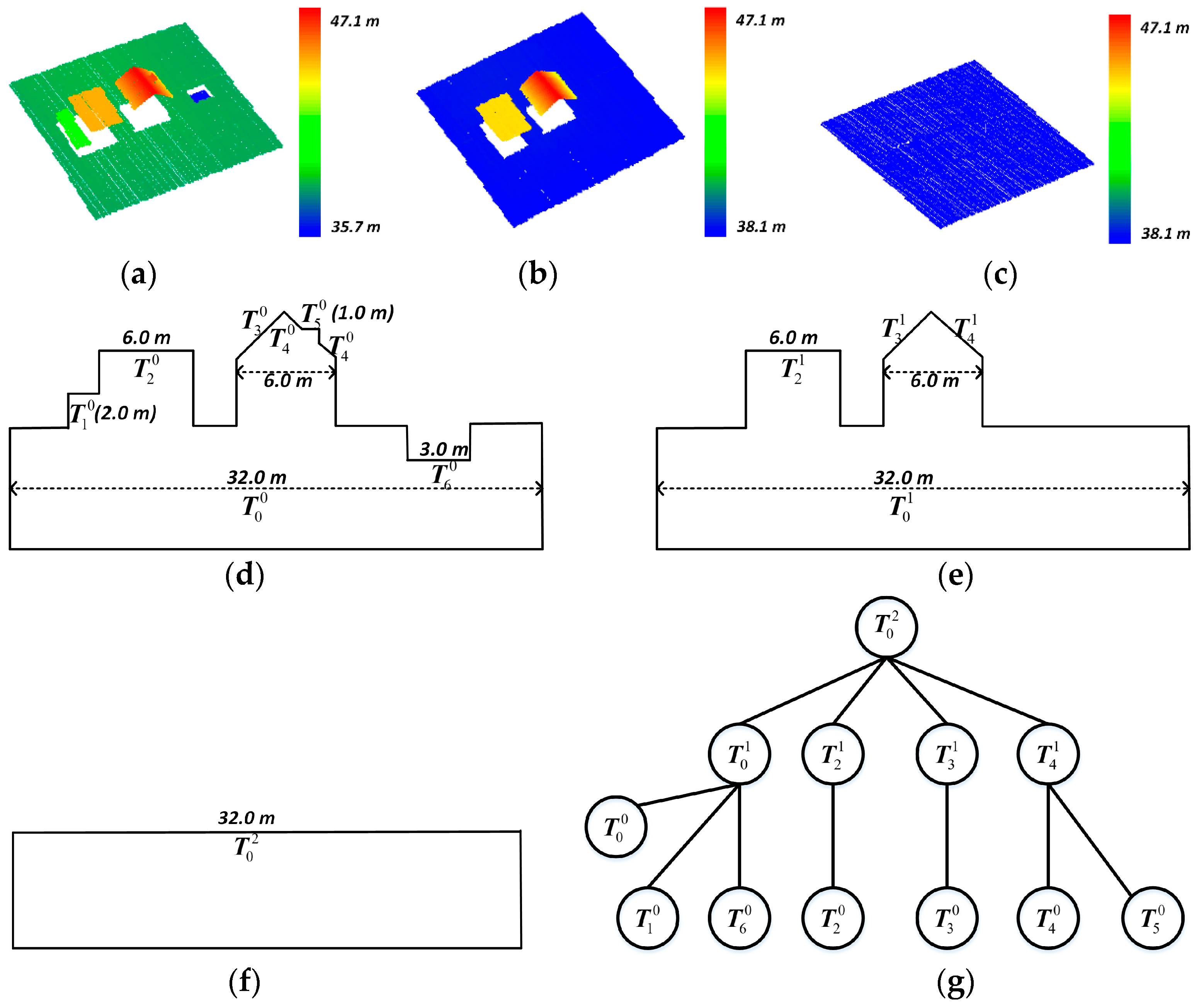
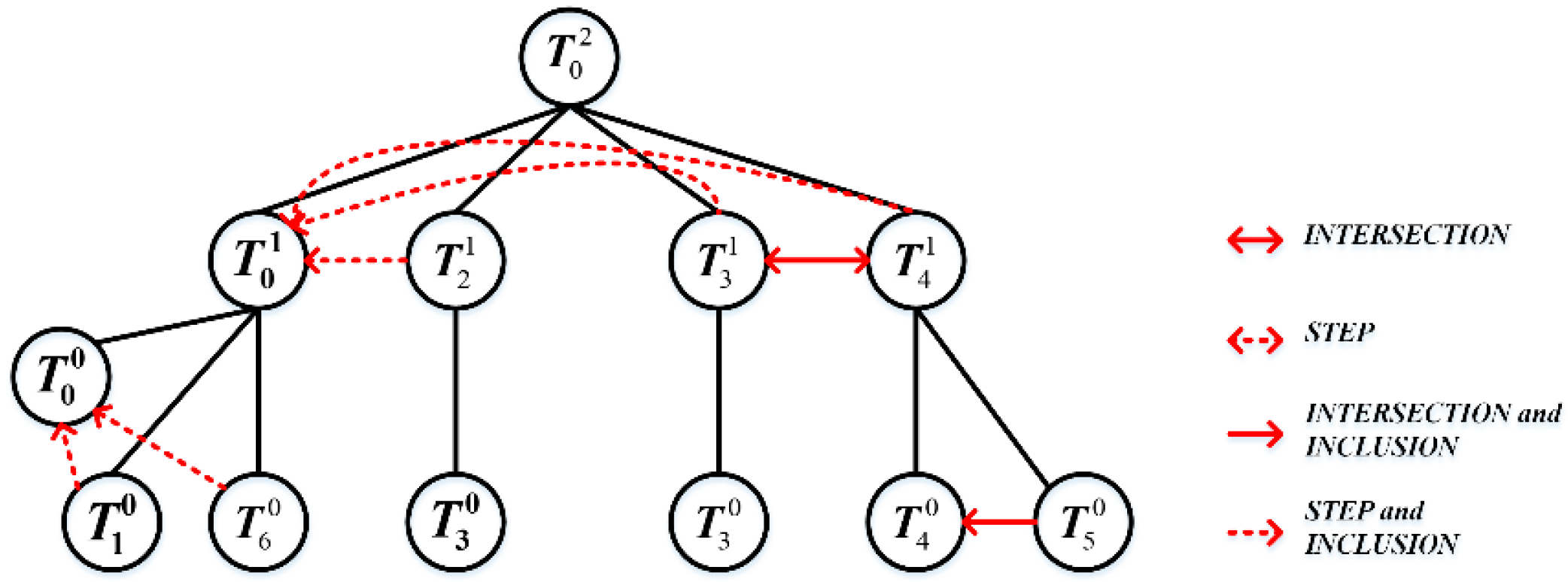
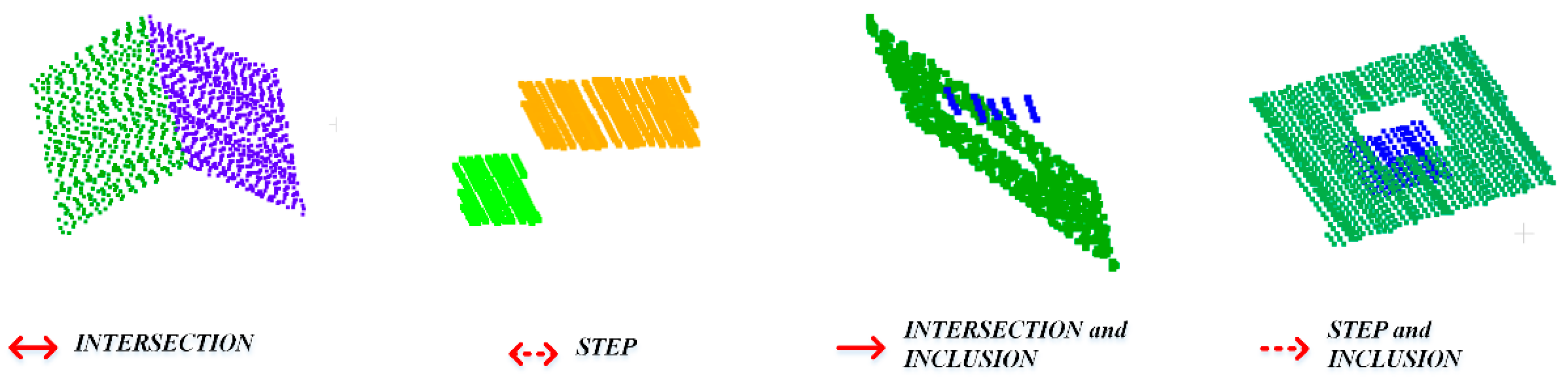
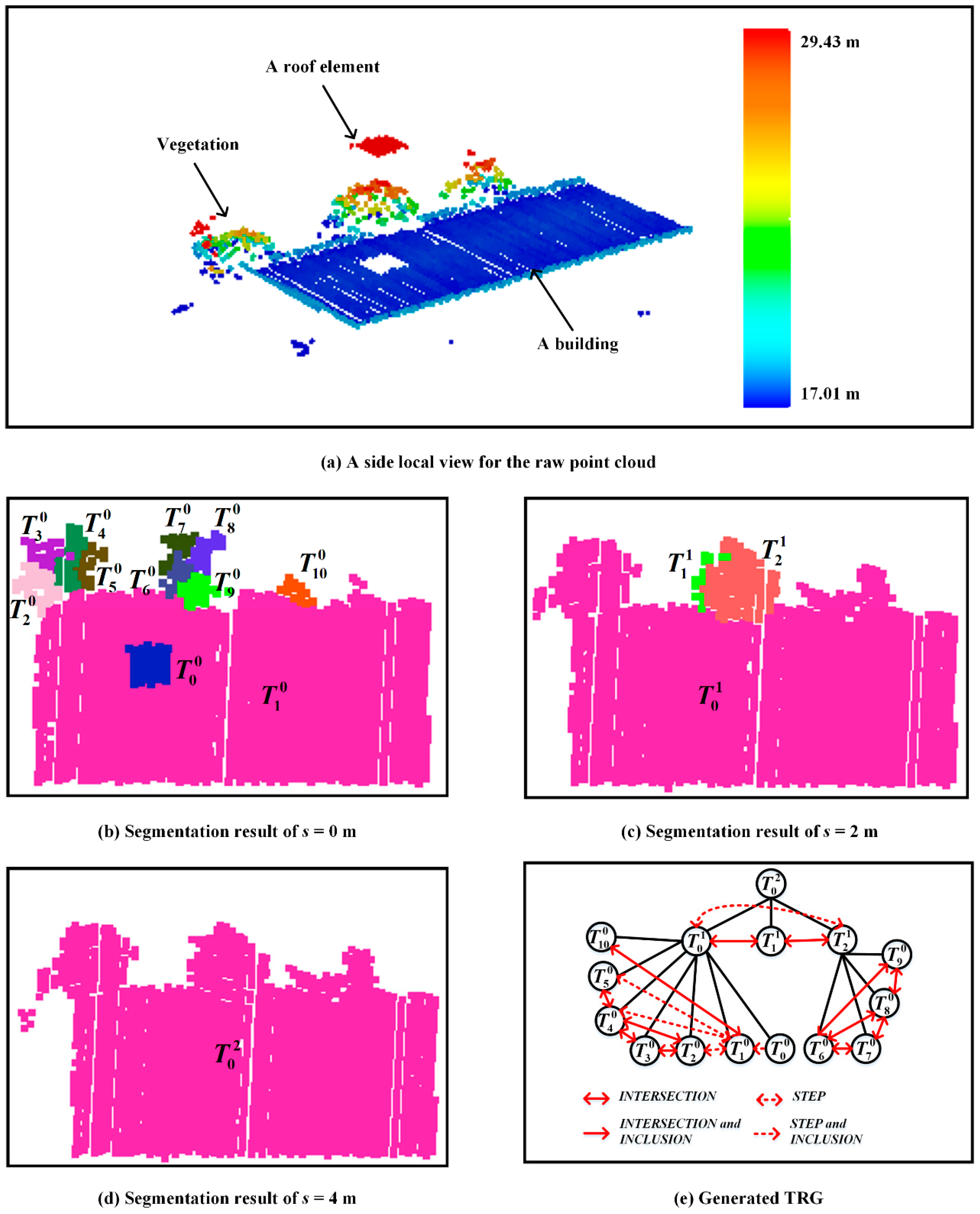
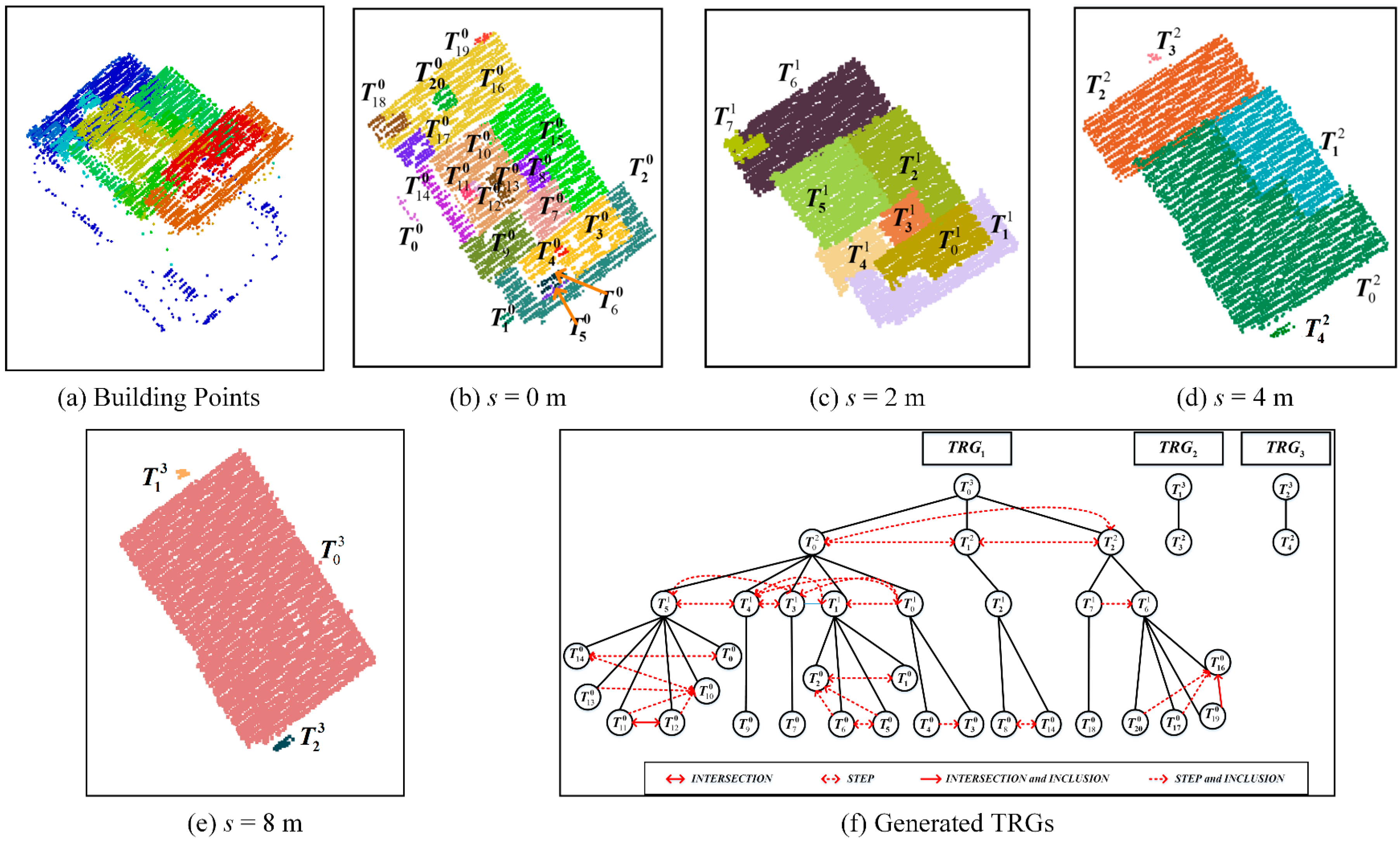
2.2. Generating the Morphological Scale Space and Constructing the Topological Relationship Graph (TRG)

To generate the scale space for an object, the improved morphological reconstruction is iteratively executed with the increasing of the scale. Hence, for one object, a scale space is constructed by employing a series of scale values ($S=\left\{s_0,s_1,s_2,\dots ,s_n\right\}$) until all points of the object are located on a horizontal plane, and each scale value indicates one level. It is clear that the points of one object have been portioned as different segments at each level. Sequentially, topological relationship graphs (TRGs) across levels can thus be created by linking the spatial relations between segments of adjacent levels, and each segment of one level is taken as a node. The rule of linking is that if most points from one segment in a fine level can be found in another segment of the next coarse level by the point index, the spatial relation between them is recorded. Figure 2 is an example of generating scale space and constructing topological relationship graphs within one building, and the scales are defined as $S=\left\{2,4,8,16,\dots \right\}$, where the former scale is half of the latter scale. Figure 2a is the raw point clouds, and Figure 2d is a corresponding cross-section. There are seven segments, and the size of each segment is annotated. Figure 2b,e are the results of the improved morphological reconstruction at the scale of 2 m. $T_1^0$, $T_5^0$ and $T_6^0$ are flattened, and $T_3^0$ and $T_4^0$ are preserved. Figure 2c,f are the final results of the improved morphological reconstruction, and the maximum scale is 4 m. Figure 2g is the generated TRG.

Moreover, the proposed method labels the topological relationship between each two adjacent segments for each level in the generated TRG, where the level is in order from the coarsest to the finest. For the labeling, four types of situations are designed, namely, INTERSECTION, STEP, INTERSECTION and INCLUSION, STEP and INCLUSION, as shown in Figure 3. The steps of labeling are described as follows:

Step 1: all segments are grouped into different clusters according to their father node. For example, segments of the third level in Figure 2g would be grouped into four clusters, which are the set of $\left\{\left\{T_0^0,T_1^0,T_6^0\right\},\left\{T_2^0\right\},\left\{T_3^0\right\},\left\{T_4^0,T_5^0\right\}\right\}$.

Step 2: arbitrary two segments in one cluster are judged whether they are neighboring in the horizontal direction. Two neighboring segments are denoted as a segment pair. For example, the cluster $\left\{T_0^0,T_1^0,T_6^0\right\}$ would result in one set of two pairs {$\left\{T_0^0,T_1^0\right\},\left\{T_0^0,T_6^0\right\}$}.

Step 3: traverses the segment pairs in each cluster one by one, derives an intersection line from the segment pair, and labels the relationship of the pair as either INTERSECTION or STEP. More specifically, if the distance between the points in the segment pair and the intersection line is less than one threshold (e.g., two times the point spacing), the relationship is labeled as INTERSECTION. Otherwise, it is labeled as STEP. On the other hand, if points of one segment are fully located in the exterior boundary of another segment in a segment pair, the relationship is labeled as INCLUSION as well. Additionally, the relationship between the segments from different clusters could be derived from their father nodes. For example, the labeled result of Figure 2g is illustrated in Figure 4.

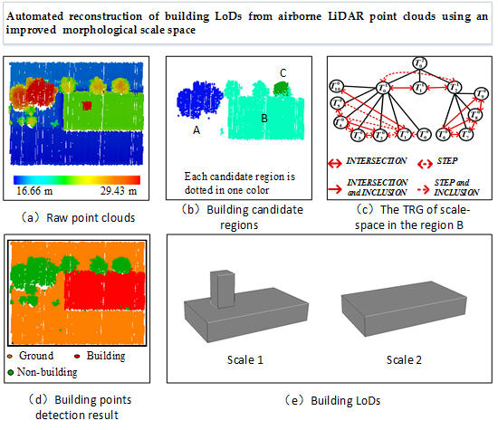
3. Generating Building Levels of Detail (LoDs) Based on the Improved Morphological Scale Space

Figure 5 illustrates the flowchart of the proposed method. Four key steps are integrated to generate 3D building LoDs from airborne laser scanning point clouds, namely, detection of building candidate regions, generation of the improved morphological scale space, detection of building points, and generation of building LoDs.

3.1. Building Candidate Region Extraction and Generation of the Morphological Scale Space

Buildings in an urban scene have different structures with highly variable sizes and stories. In general, the maximum scale is determined by their sizes and structures in the scale space. That is to say, different buildings may be assigned different values for the maximum scales. Hence, the candidate region of each building is first detected from the point clouds for adaptively tuning the maximum value, and then the morphological scale space is generated for each candidate region respectively.

Step 1: The filtering method of [36] is utilized to separate ground points from non-ground points. The filtering method classifies the points into a set of segments and one set of individual points by point cloud segmentation, which are filtered by segment-based filtering and multi-scale morphological filtering, respectively. Therefore, the non-ground points include two sets, non-ground segments and non-ground individual points. Figure 6b is the filtering result of Figure 6a, and Figure 6c is the non-ground segments.

Step 2: Extract the candidate region of each building. First, the non-ground segments are clustered via a region-growing method with the constraint of two-dimensional Euclidean distance, and the distance threshold is specified as two times that of the point spacing. Then, with the assumption that one building has a certain area, width and large elevation differences with its neighboring terrain areas, the clusters are classified by Equation (10) to obtain the candidate building clusters. Finally, each candidate building cluster is buffered with a distance (e.g., 3 m) to obtain a buffer area, which is regarded as the candidate region of each building object. The buffer operator aims to ensure the completeness of an object. For example, Figure 6d is the result of extracting candidate regions.

$$cBuilds=\left\{S{C}_i\in SC|\begin{array}{c}Rule1:Num\left(Bound\left(S{C}_i\right)>t_H\right)>0.25\times Num\left(Bound\left(S{C}_i\right)\right)\&\&\\ Rule2:Width\left(S{C}_i\right)>t_W\&\&\\ Rule3:Area\left(S{C}_i\right)>t_A\end{array}\right\}$$

(10)

where $cBuilds$ denotes the candidate building clusters; $SC$ is the set of clusters, and $S{C}_i$ is the ith cluster; $Bound()$ is used to extract boundary points of each cluster; $Num()$ is a counter of points satisfying the condition of the elevation difference; $Width()$ and $Area()$ calculate the width and area of a cluster; $t_W$, $t_A,$ $t_H$ are three thresholds of the width, area and elevation difference respectively. $t_W$ and $t_A$ should be tuned according to the scene (e.g., a modern megacity or a village), where $t_A$ could be specified as 2.0–100.0 m², and $t_W$ could be specified as 2.0–10.0 m. $t_H$ could be specified as a value in consideration of a building no lower than 1.5 m.

Step 3: Generate the morphological scale space and the corresponding TRGs. Once the candidate region of one building object is determined, the morphological scale space is generated according to Section 2, and the corresponding TRGs are recorded as well. Generally, the root of a TRG represents the entire object region, and the leaf nodes of a TRG are the segments of an object region in the minimum scale. The relationships between segments from the same level are also labeled in the generated TRG. For the generation of the morphological scale space, in consideration of time efficiency, a set of scales $S=\left\{2,4,8,16,\dots \right\}$ is specified for iteratively generating each level of scale space, whereby the former scale value is half of the later. An example is illustrated in Figure 7.

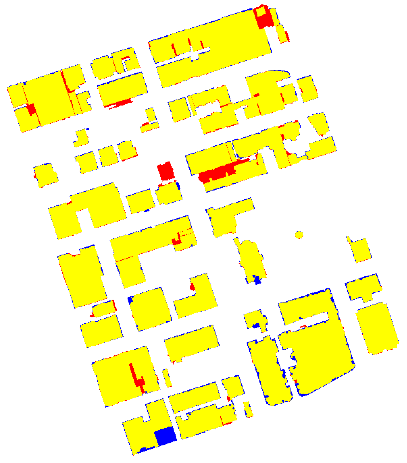
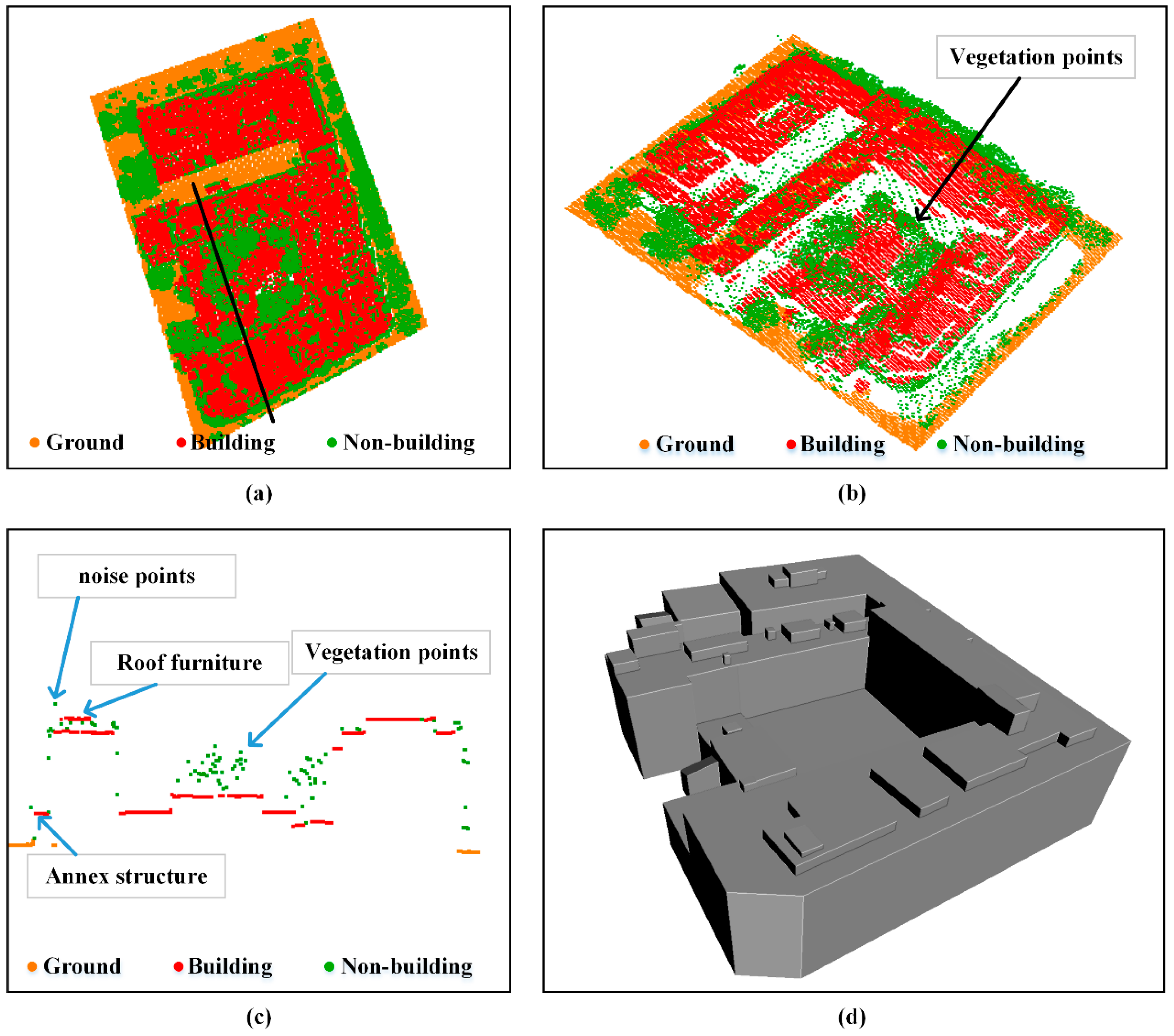
3.2. Building Point Detection

A method based on the generated TRGs is employed to extract building points from each building candidate region. The method distinguishes buildings from other points in consideration of the entire object and its changes across scales. The method includes two steps. The first step is to label the building TRGs, and the second step is to remove non-building points from the building TRG.

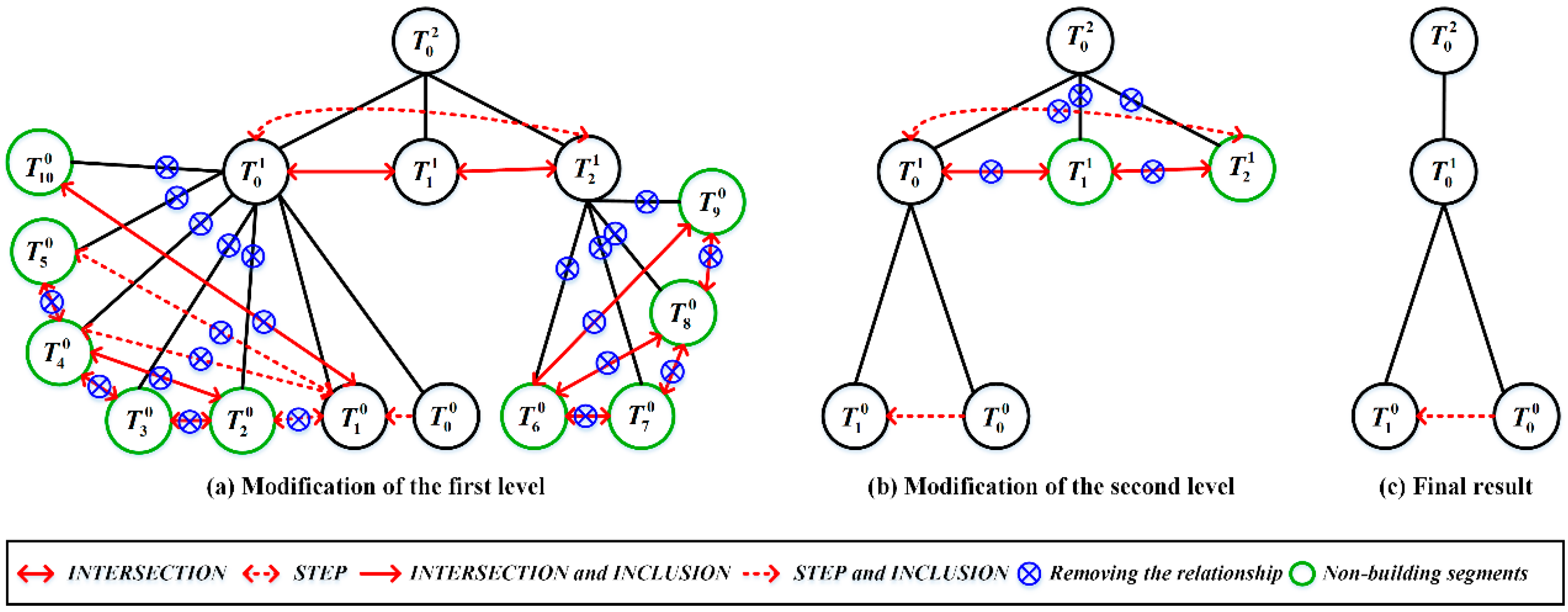
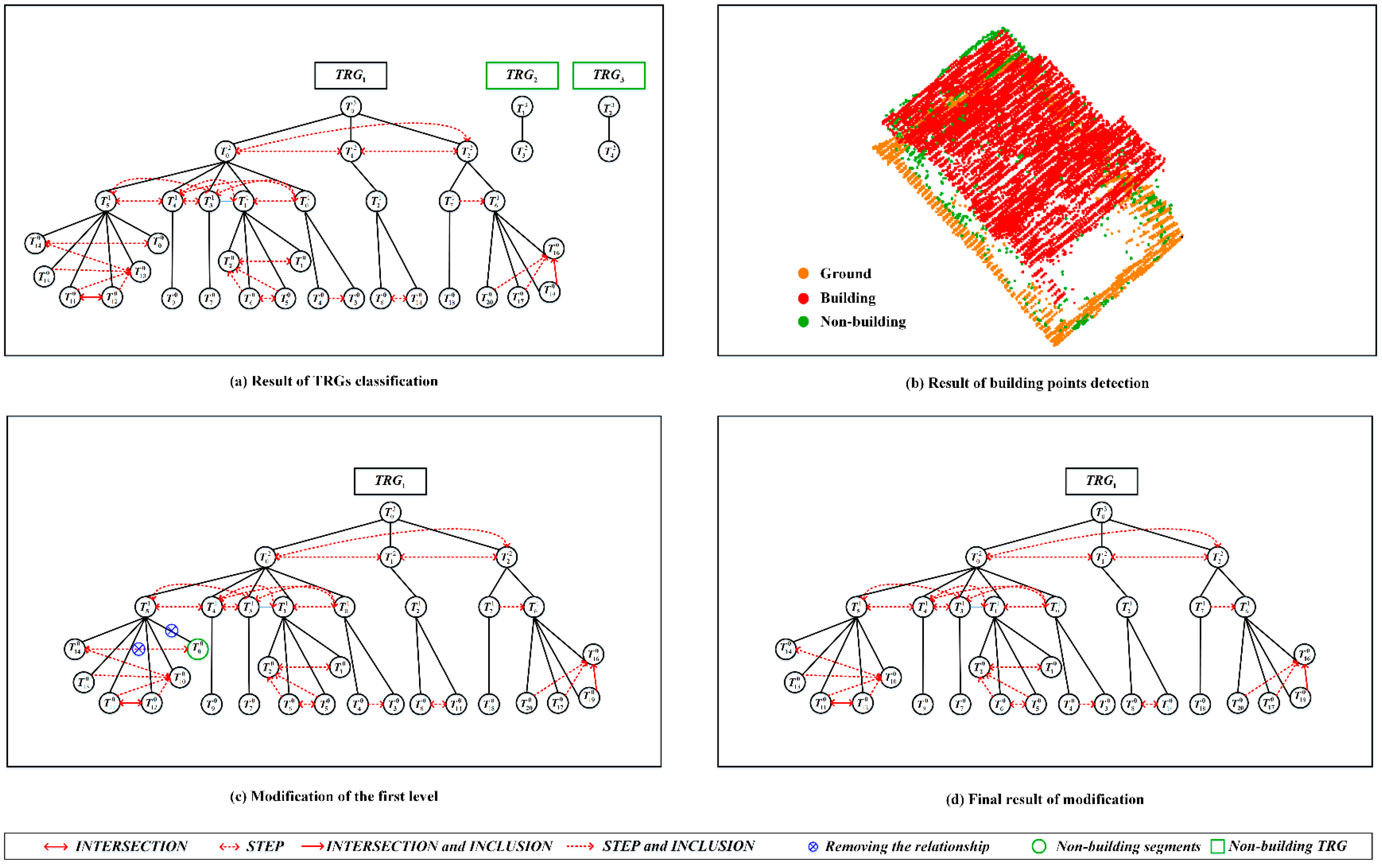
3.2.1. Classification of TRGs

The method first classifies all TRGs into building TRGs and non-building TRGs by five features, as listed in

Table 1. Five features based on the TRG.

Features	Descriptions	Characteristics
The area of the TRG ($A$)	The area of the TRG	The areas of buildings and large trees are large, and the areas of small objects (e.g., vehicles, low vegetation and street furniture) are small
The width of the TRG ($W$)	The width of the TRG	The widths of buildings and large trees are large, and the widths of small objects (e.g., vehicles, low vegetation and street furniture) are small
The area ratio of the segments ($A{R}_{MIN-MAX}$)	The value is the ratio between the minimum and the maximum area of segments across scales. It reflects the result of segmentation for objects in different scales	The value of a building is large, and that of a tree may be small
The area ratio of ground points ($A{R}_{G-O}$)	The ratio in areas between the entire object and the ground points in the corresponding region. It reflects the penetrating capacities in different objects	The value of a building generally approximates zero, and it may be higher in the area of vegetation
The ratio of segmented points ($PN{R}_{MIN-MAX}$)	The ratio in the number of segmented points between the minimum scale and the maximum scale. It reflects the changing of surface characteristics across scales and the penetrating capacities in different objects	The value of a building is large, and it is small for vegetation

. The five features are mainly related to geometrical sizes, surface characteristics, the penetrating capacities within different objects, and the changing characteristics of objects across scales. The classification rules are defined in Equation (11). For example, Figure 6e is the result of TRG classification.

$$buildTRGs=\left\{pTR{G}_i\in ATRGs|\begin{array}{c}Rule1:A>t_A\&\&\\ Rule2:W>t_W\&\&\\ \begin{array}{c}Rule3:A{R}_{MIN-MAX}>t_{ARMM}\&\&\\ Rule4:A{R}_{G-O}<t_{ARGO}\&\&\\ Rule5:PN{R}_{MIN-MAX}>t_{PNRMM}\end{array}\end{array}\right\}$$

(11)

where $buildRegions$ is the set of building TRGs, $ATRGs$ is the set of all TRGs, $pTR{G}_i$ is $i\mathrm{th}$ TRG, $t_A$, $t_W$, $t_{ARMM}$, $t_{ARGO}$ and $t_{PNRMM}$ are thresholds of five features, respectively. The threshold $t_{ARMM}$ should be determined by several factors, such as the flatness of an object. Generally, it should not be lower than 0.5. For the threshold $t_{ARGO}$, in theory, it should be near zero. However, because of the structure and material of a building, there may be a lot of ground points below roofs. Therefore, the value of $t_{ARGO}$ ranges from 0.2 to 0.6. The threshold of $t_{PNRMM}$ is mainly relevant to the penetrating capacity and the surface characteristics, and it could be larger than 0.5.

3.2.2. Extraction of the Final Building Points from Each Building TRG

Although TRGs have been classified, there may be some other objects (e.g., vegetation, vehicles) in the building TRGs, and these objects should be removed. Generally, these objects consist of small segments or individual points in the minimum scale, and they are near the border of the building region. Therefore, the process is described as follows.

Step 1: The method detects the small segments by an area threshold $t_{SA}$ in the minimum scale, and non-ground points removed in the process of segmentation are also detected. The detected points are labeled as unclassified points. Generally, the threshold $t_{SA}$ is specified as 3.0–5.0 m².

Step 2: The unclassified points are grouped into different clusters by a region-growing method with the constraint of two-dimensional Euclidean distance.

Step 3: For each cluster, the distance between its boundary and the border of the building region is calculated. And then, the cluster will be determined whether it locates inside the building region or near the border of the building region by one distance threshold, which is also specified as two times that of the point spacing. If a cluster locates inside the building region, it would be classified as building. Otherwise, five features are calculated after reconstructing a new TRG for each unclassified cluster, and each unclassified cluster is labeled as building or non-building by Equation (11).

Figure 6f is the result of extracting the final building points of Figure 6a. Two trees near the building are removed. Based on the detection result, the nodes of non-building segments would be removed from the finest level to the coarsest level, and the relationships of these segments are also removed at the same time. The process is illustrated in Figure 8. Moreover, if there are non-building child nodes, the non-building points should also be removed the father node. For example, points of $T_{10}^0$ should be removed from the segments $T_0^1$ and $T_0^2$.

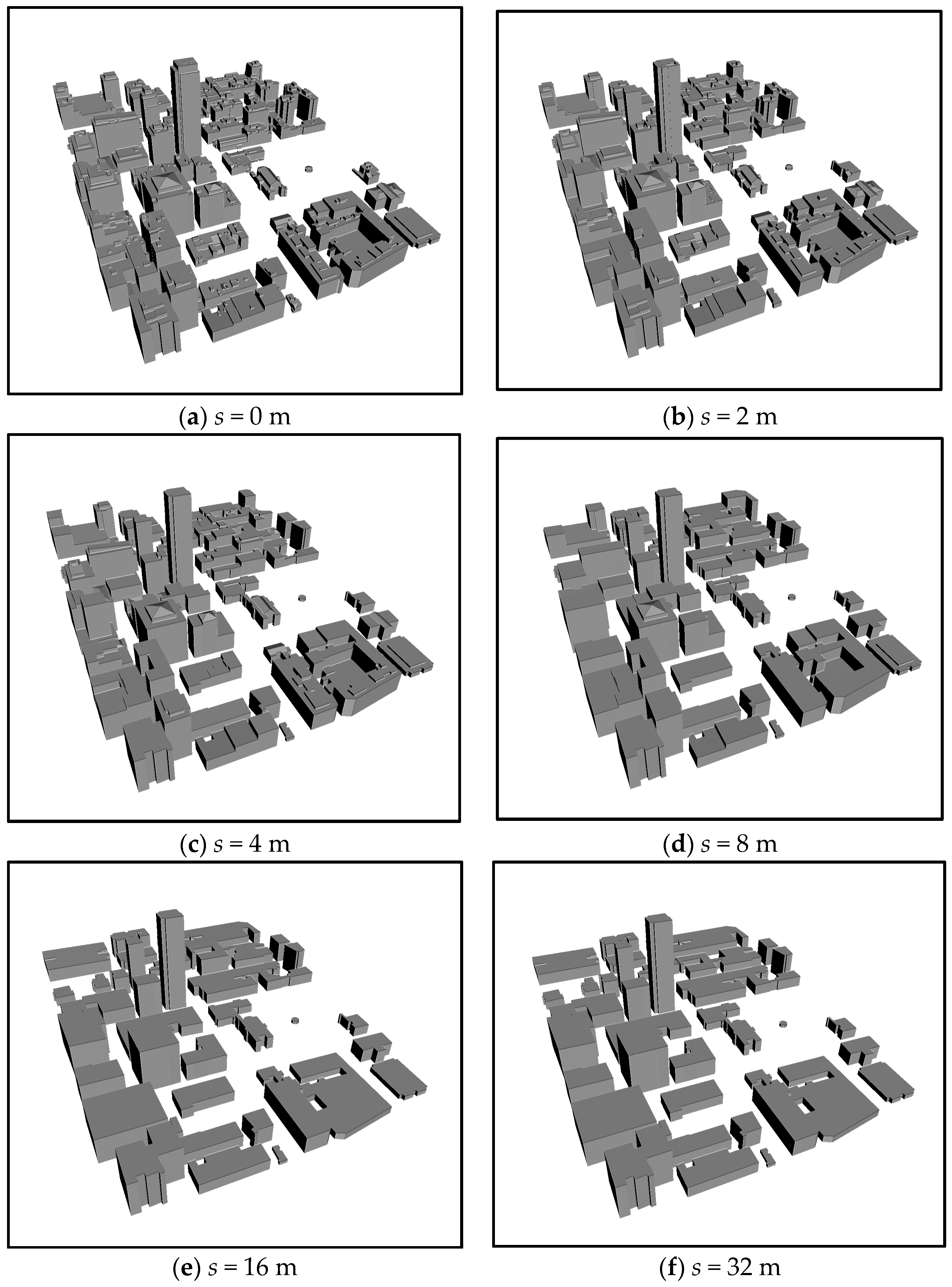
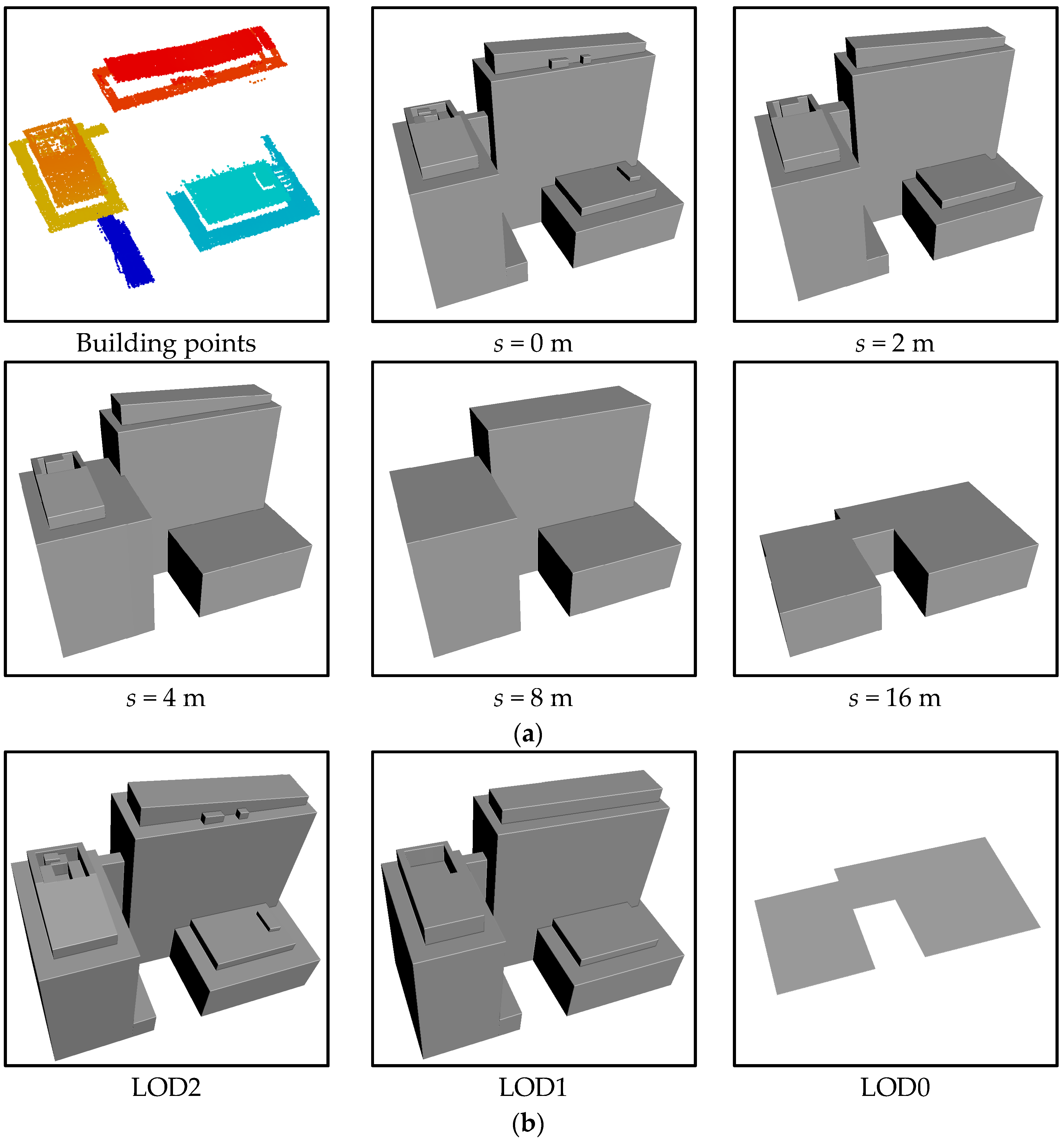
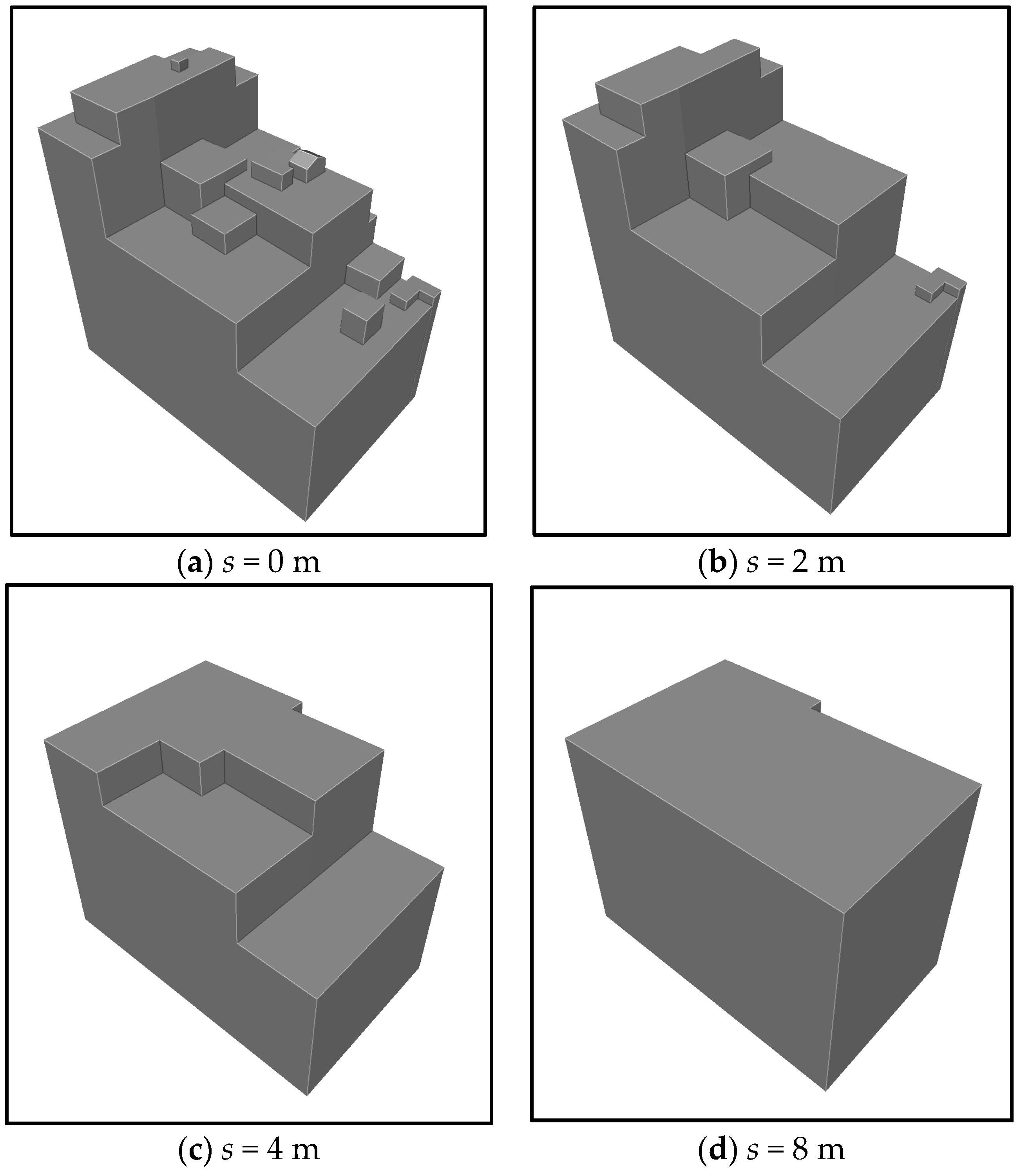
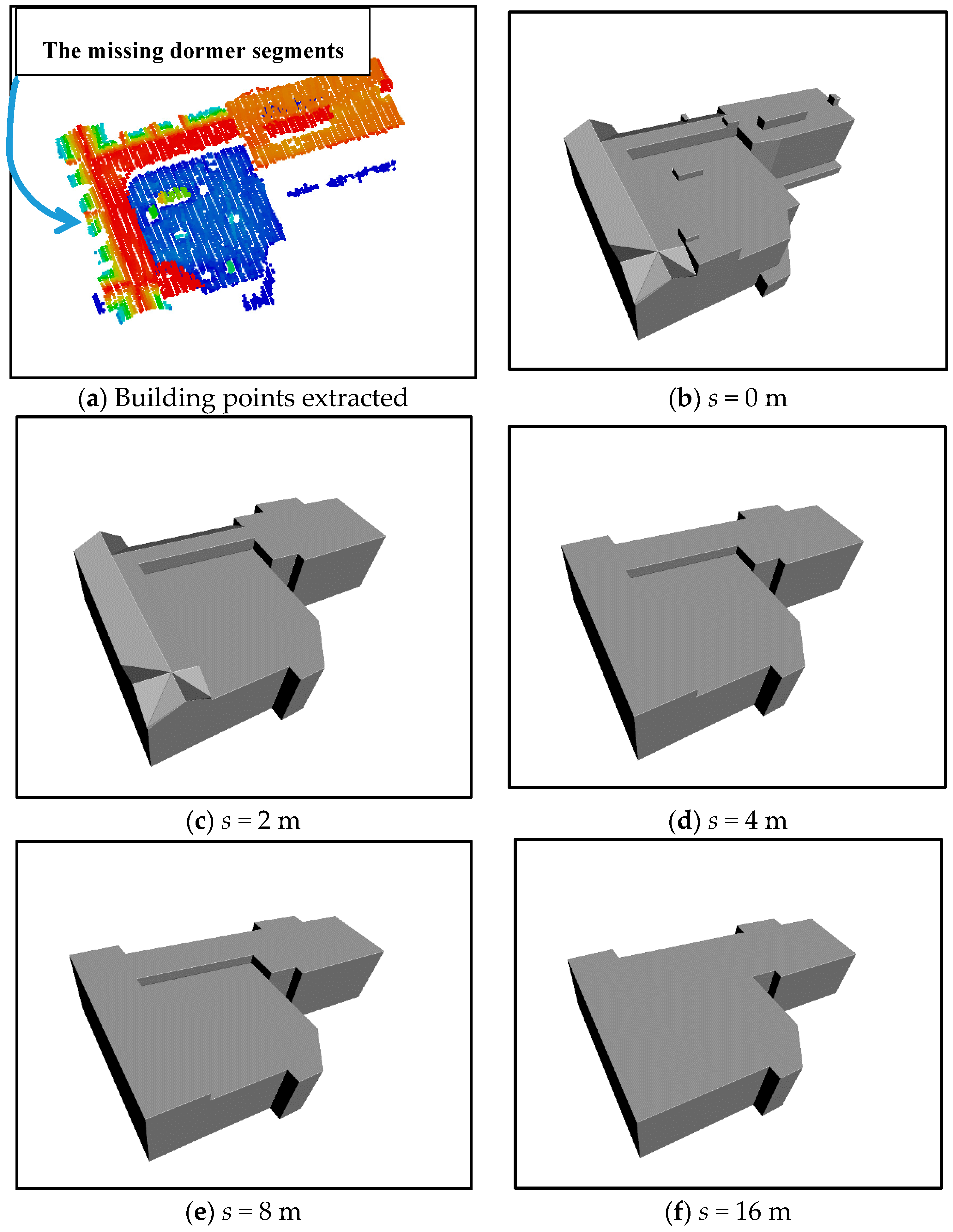
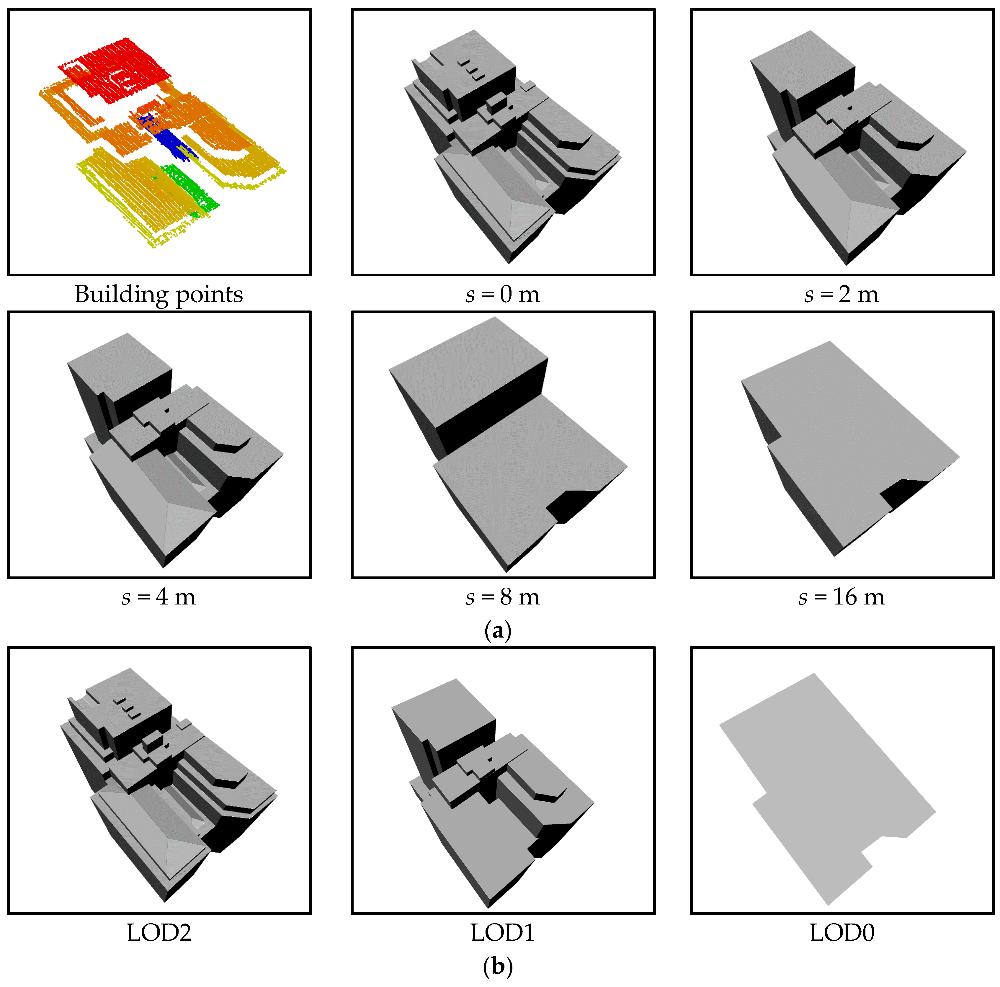
3.3. Building LoD Generation

After automatically extracting building points and modifying the corresponding TRG, the method reconstructs each building in each scale by the cycle graph analysis method of [37] to obtain the corresponding building LoDs. The main steps of reconstructing a building model are as follows. First, a graph about the topological relationship between each two adjacent segments from the same level is constructed, and it is derived from the labeled TRG. Simultaneously, the feature lines are also derived from each two adjacent segments. Then, roof corners are obtained by a strategy for detecting closed cycles in the graph. The corner points are used to fix the ending points of the corresponding feature lines. Finally, one building model is reconstructed by the combination of feature lines. Two cases are illustrated in

Table 2. First example of generating the LoDs for the building of Figure 6.

Scale Values	Multi-Scale Roof Data	Plane Segmentation Results	Building LoDs
0 m
2 m

and

Table 3. Second example of generating the LoDs for a building with gable roofs and dormers.

Scale Values	Multi-Scale Roof Data	Plane Segmentation Results	The Final TRG	Building LoDs
0 m
2 m
4 m

.

4. Experimental Results and Analysis

The experiment was conducted on the Toronto dataset (as shown in Figure 9) provided by International Society for Photogrammetry and Remote Sensing (ISPRS) to validate the performance of the proposed method. The area of this dataset is about 403 m × 532 m, and the elevation ranges from 40 to 190 m. There are 58 buildings larger than 2.5 m², and the corresponding building area is 88,249.8 m². The dataset is located in a commercial zone with representative scene characteristics of a modern megacity. Moreover, the area is covered by the high-rise and multi-story buildings with complex rooftop structures, which are very suitable for verifying the proposed method.

The procedure of the proposed method was executed to extract building points and generate the LoDs for each building. The parameters involved in the proposed method are listed in

Table 4. Parameter settings.

Parameters	Values	Description	Steps
$t_A$/m2	50	The area threshold	Building candidate region extraction
$t_W$/m	5	The width threshold
$t_H$/m	1.5	The threshold of describing the elevation difference between the boundary points of a building and the DEM
$t_N$	10	This parameter is used to remove very small segments in plane segmentation	The generation of the scale space
$t_S$/°	10	A threshold for the slope parameter
$t_{SH}$/m	0.2	It is a threshold of the elevation difference for determining a segment is inclined or horizontal after morphological reconstruction
$t_{ARMM}$	0.5	The area ratio of the segments across levels of a TRG	Building point detection
$t_{ARGO}$	0.5	The area ratio of ground points within a TRG
$t_{PNRMM}$	0.5	The ratio of segmented points across levels of a TRG
$t_{SA}$/m2	5	An area threshold for detecting small segments near buildings

. The point clouds were first filtered into non-ground points and ground points. The result is shown in Figure 10a, and the non-ground segments are showed in Figure 10b. Then, building candidate regions were extracted, as illustrated in Figure 10c. For each building candidate region, the improved morphological scale space and the labeled TRG were generated, TRGs were classified, and building points were detected, as shown in Figure 10d–f. Then, the building LoDs were reconstructed. Figure 11, Figure 12 and Figure 13 are the processes for extracting building points and reconstructing building LoDs from the building candidate region PB of Figure 10c. The result of reconstructing the building LoDs for the entire scene is shown in Figure 14. It can be seen that roof structures change from complicated to simple with the increasing scale until each roof becomes a plane. Therefore, the reconstructed building models at different LoDs can serve various urban monitoring and analysis applications. Moreover, the number of levels for each building self-adapts to its size and roof structures, ranging from three levels to six levels. More importantly, the proposed method can reconstruct the roof model with any one scale from the finest building points by the morphological reconstruction. The coarser roof model does not need to be generated from the finest roof model. For example, the proposed method could directly generate the level s = 4 m from the raw building points. This is very helpful to save the cost and satisfy the user’s requirement.

The high quality of building point detection results was the prerequisite for reconstructing building LoDs in a scene. Hence, the result of building point detection was submitted to the organization ISPRS for evaluation [38]. The evaluation result is shown in Figure 15, and the details can be found on the website [39]. Several indicators are adopted for quantitative evaluation, including Completeness ($CP$), Correctness ($CR$) and Quality ($Q$) at the pixel or object level, and the total Root Mean Square (RMS) of reference boundaries. The result is listed in

Table 5. Evaluation result by ISPRS; the best results are highlighted.

Methods	Per_Area/%			Per_Object/%			RMS/m
	CP	CR	Q	CP	CR	Q
The proposed method	94.7	95.5	90.6	98.3	96.6	95.0	0.8
WHUY2 [34]	95.1	89.3	85.4	96.6	94.6	91.6	1.2
TUM [41]	85.1	80.0	70.1	86.2	92.3	80.4	1.6
FIE [40]	96.6	90.6	87.8	98.3	98.2	96.6	1.2
ITCM [42]	80.5	82.1	68.5	96.6	22.9	22.7	1.5
MAR2 [15]	93.7	94.9	89.2	98.3	94.9	93.4	2.8
MON2 [43]	95.1	91.1	87.0	100	83.6	83.6	1.1
Z_GIS [44]	93.0	94.5	88.2	96.6	96.5	93.3	1.0
MIN	80.5	80	68.5	86.2	22.9	22.7	0.8
MAX	96.6	95.5	90.6	100	98.2	96.6	2.8

. It can be seen that the Correctness values are 95.5% at the pixel level, and 96.6% at the object level. The high values show that the proposed method can robustly distinguish buildings from vegetation or other objects. It may benefit from the combination of features derived from the local and the whole of an object. In this result, there are only two false positives at the object level. The false positives are large objects with smooth surfaces, which are very easily classified as buildings. The Completeness values are 94.7% at the pixel level, and 98.3% at the object level. The values indicate the method could robustly extract buildings, as shown in the yellow areas of Figure 15. Additionally, the proposed method could also preserve annex structures and rooftop furniture well by taking large parts of the building and small structures as a whole in the process of detecting buildings, and robustly removing noise and vegetation points on the roofs, as illustrated in Figure 16. In order to further analyze the performance of the proposed method, the comparison between the proposed method and the other methods [13] is listed in Table 5, showing that the proposed method has the best qualities in detecting buildings at the pixel level and the total RMS, and only the method of FIE [40] obtained a better performance than the proposed method at the object level. Therefore, the result of building point detection could provide a good foundation for the reconstruction of building LoDs. However, some small segments near the boundary of a building may be erroneously removed, as shown in Figure 15 (dotted in blue), thereby resulting in incorrect building LoDs reconstruction. Figure 17 shows an example of reconstructing building LoDs for a building with complex rooftop structure. Because the points of dormers are few, they failed to be detected, as illustrated in Figure 17a. The model of s = 0 m also missed several dormers, as shown in Figure 17b.

Finally, we selected two cases to describe the results of reconstructing building LoDs in the local view, and the results were compared with the building LoDs in the framework of CityGML. The first case is a connected building in Figure 18, where there is an ensemble of three parts with annex structures and roof furniture. Figure 18a is the result of the proposed method, and Figure 18b is the result based on CityGML. It shows that the proposed method could find the corresponding model matching to each level of building LoDs based on CityGML. For example, the model of s = 0 m is the same with LoD2, the model of s = 2 m approximates LoD1, and the model of s = 16 m is similar to the LoD0, where only the elevation of the model of s = 16 m is assigned the minimum elevation of the building points. Moreover, the models based on CityGML have only three levels, but the models of the proposed method have five levels with a more gradual change for reducing the difference between two adjacent levels. In the visualization of multi-scale representations for a building, the result of the proposed method could have a smaller jump between two adjacent levels. The second case is a building with multiple stories, where there are various types of roof structures (e.g., flat roofs and gable roofs), as shown in Figure 19. Figure 19a is the result of the proposed method, and Figure 19b is the result based on the CityGML. It also shows the models of the proposed method have a smaller change between two adjacent levels. In addition, the inclined roofs are preserved in the model of s = 2 m from the proposed method, while each roof is flat in the LoD1 of the CityGML.

5. Conclusions

In this study, we propose a method to reconstruct building levels of detail (LoDs) by using an improved morphological scale-space. After separating ground and non-ground points, the candidate region of each building is detected. The scale-space of each building candidate region is obtained by iteratively using the improved morphological reconstruction. Topological relationship graphs (TRGs) are generated by relinking the relationships of segments between two adjacent scales. Then, building points are detected by features based on TRG, and the TRG will be modified after detection. Finally, the proposed method reconstructs the roof model for each building at each scale. To verify the validities and the robustness of the proposed method, the Toronto dataset from International Society for Photogrammetry and Remote Sensing (ISPRS) was selected to extract building points and reconstruct building LoDs. The results of building point detection were submitted to ISPRS for evaluation, and the building LoDs were compared with the building LoDs based on the CityGML. The results demonstrate that the proposed method has a good performance in robustly extracting the buildings with details (e.g., roof furniture) and distinguishing buildings from vegetation or other objects. More importantly, the proposed method can directly reconstruct building LoDs from airborne Light Detection and Ranging (LiDAR) point clouds with the adaptive number of levels while maintaining the spatial relations between adjacent levels. However, some small parts of buildings may be missed, which affects the quality of building LoDs. In the future, we will incorporate spatial reasoning to improve the performance of extracting building details.

References

1. Gröger, G.; Kolbe, T.H.; Nagel, C.; Häfele, K.H. OGC City Geography Markup Language (CityGML) Encoding Standard; Open Geospatial Consortium: Wayland, MA, USA, 2012. [Google Scholar]
2. Jochem, A.; Hofle, B.; Rutzinger, M.; Pfeifer, N. Automatic roof plane detection and analysis in airborne lidar point clouds for solar potential assessment. Sensors 2009, 9, 5241–5262. [Google Scholar] [CrossRef] [PubMed]
3. Biljecki, F.; Ledoux, H.; Stoter, J.; Zhao, J. Formalisation of the level of detail in 3D city modelling. Comput. Environ. Urban Syst. 2014, 48, 1–15. [Google Scholar] [CrossRef]
4. Fan, H.; Meng, L. A three-step approach of simplifying 3D buildings modeled by CityGML. Int. J. Geogr. Inf. Sci. 2012, 26, 1091–1107. [Google Scholar] [CrossRef]
5. Forberg, A. Generalization of 3D building data based on a scale-space approach. ISPRS J. Photogramm. Remote Sens. 2007, 62, 104–111. [Google Scholar] [CrossRef]
6. Mao, B.; Ban, Y.; Harrie, L. A multiple representation data structure for dynamic visualisation of generalised 3D city models. ISPRS J. Photogramm. Remote Sens. 2011, 66, 198–208. [Google Scholar] [CrossRef]
7. Thiemann, F.; Sester, M. Segmentation of buildings for 3D-generalisation. In Proceedings of the ICA Workshop on Generalisation and Multiple Representation, Leicester, UK, 20–21 August 2004.
8. Kada, M. 3D building generalization based on half-space modeling. Int. Arch. Photogramm. Remote Sens. Spat. Inf. Sci. 2006, 36, 58–64. [Google Scholar]
9. Sester, M. Generalization based on least squares adjustment. Int. Arch. Photogramm. Remote Sens. Spat. Inf. Sci. 2000, 33, 931–938. [Google Scholar]
10. Biljecki, F.; Ledoux, H.; Stoter, J. An improved LOD specification for 3D building models. Comput. Environ. Urban Syst. 2016, 59, 25–37. [Google Scholar] [CrossRef]
11. Verdie, Y.; Lafarge, F.; Alliez, P. LOD Generation for urban scenes. ACM Trans. Graph. 2015, 34, 1–14. [Google Scholar] [CrossRef]
12. Shan, J.; Toth, C.K. Topographic Laser Ranging and Scanning, Principles and Processing; CRC Press: London, UK, 2008; Volume 15, pp. 423–446. [Google Scholar]
13. Rottensteiner, F.; Sohn, G.; Gerke, M.; Wegner, J.D.; Breitkopf, U.; Jung, J. Results of the ISPRS benchmark on urban object detection and 3D building reconstruction. ISPRS J. Photogramm. Remote Sens. 2014, 93, 256–271. [Google Scholar] [CrossRef]
14. Tomljenovic, I.; Höfle, B.; Tiede, D.; Blaschke, T. Building extraction from airborne laser scanning data, an analysis of the state of the art. Remote Sens. 2015, 7, 3826–3862. [Google Scholar] [CrossRef]
15. Mongus, D.; Lukač, N.; Žalik, B. Ground and building extraction from LiDAR data based on differential morphological profiles and locally fitted surfaces. ISPRS J. Photogramm. Remote Sens. 2014, 93, 145–156. [Google Scholar] [CrossRef]
16. Jochem, A.; Höfle, B.; Wichmann, V.; Rutzinger, M.; Zipf, A. Area-wide roof plane segmentation in airborne LiDAR point clouds. Comput. Environ. Urban Syst. 2012, 36, 54–64. [Google Scholar] [CrossRef]
17. Zhao, Z.; Duan, Y.; Zhang, Y.; Cao, R. Extracting buildings from and regularizing boundaries in airborne lidar data using connected operators. Int. J. Remote Sens. 2016, 37, 889–912. [Google Scholar] [CrossRef]
18. Xu, S.; Vosselman, G.; Oude Elberink, S. Multiple-entity based classification of airborne laser scanning data in urban areas. ISPRS J. Photogramm. Remote Sens. 2014, 88, 1–15. [Google Scholar] [CrossRef]
19. Zhang, J.; Lin, X.; Ning, X. SVM-based classification of segmented airborne LiDAR point clouds in urban areas. Remote Sens. 2013, 5, 3749–3775. [Google Scholar] [CrossRef]
20. Chehata, N.; Guo, L.; Mallet, C. Airborne lidar feature selection for urban classification using random forests. Int. Arch. Photogramm. Remote Sens. Spat. Inf. Sci. 2009, 39, 207–212. [Google Scholar]
21. Niemeyer, J.; Rottensteiner, F.; Soergel, U. Contextual classification of lidar data and building object detection in urban areas. ISPRS J. Photogramm. Remote Sens. 2014, 87, 152–165. [Google Scholar] [CrossRef]
22. Guo, B.; Huang, X.; Zhang, F.; Sohn, G. Classification of airborne laser scanning data using JointBoost. ISPRS J. Photogramm. Remote Sens. 2015, 100, 71–83. [Google Scholar] [CrossRef]
23. Gu, Y.; Wang, Q.; Xie, B. Multiple kernel sparse representation for airborne LiDAR data classification. IEEE Trans. Geosci. Remote Sens. 2016, 1–21. [Google Scholar] [CrossRef]
24. Awrangjeb, M.; Fraser, C. Automatic segmentation of raw LIDAR data for extraction of building roofs. Remote Sens. 2014, 6, 3716–3751. [Google Scholar] [CrossRef]
25. Richter, R.; Behrens, M.; Döllner, J. Object class segmentation of massive 3D point clouds of urban areas using point cloud topology. Int. J. Remote Sens. 2013, 34, 8408–8424. [Google Scholar] [CrossRef]
26. Sánchez-Lopera, J.; Lerma, J.L. Classification of lidar bare-earth points, buildings, vegetation, and small objects based on region growing and angular classifier. Int. J. Remote Sens. 2014, 35, 6955–6972. [Google Scholar] [CrossRef]
27. Yan, J.; Zhang, K.; Zhang, C.; Chen, S.-C.; Narasimhan, G. Automatic construction of 3-D building model from Airborne LIDAR data through 2-D snake algorithm. IEEE Trans. Geosci. Remote Sens. 2015, 53, 3–14. [Google Scholar]
28. Ullman, S.; Vidal-Naquet, M.; Sali, E. Visual features of intermediate complexity and their use in classification. Nat. Neurosci. 2002, 5, 682–687. [Google Scholar] [CrossRef] [PubMed]
29. Goutsias, J.; Vincent, L.; Bloomberg, D.S. Mathematical Morphology and Its Applications to Image and Signal Processing; Computational Imaging and Vision; Kluwer: Dordrecht, The Netherlands, 2000. [Google Scholar]
30. Jung, C.R.; Scharcanski, J. Adaptive image denoising and edge enhancement in scale-space using the wavelet transform. Pattern Recognit. Lett. 2003, 24, 965–971. [Google Scholar] [CrossRef]
31. Lopez-Molina, C.; De Baets, B.; Bustince, H.; Sanz, J.; Barrenechea, E. Multiscale edge detection based on Gaussian smoothing and edge tracking. Knowl. Based Syst. 2013, 44, 101–111. [Google Scholar] [CrossRef]
32. Vincent, L. Morphological grayscale reconstruction in image analysis, applications and efficient algorithms. IEEE Trans. Image Process. 1993, 2, 176–201. [Google Scholar] [CrossRef] [PubMed]
33. Vu, T.T.; Yamazaki, F.; Matsuoka, M. Multi-scale solution for building extraction from LiDAR and image data. Int. J. Appl. Earth Obs. Geoinf. 2009, 11, 281–289. [Google Scholar] [CrossRef]
34. Yang, B.; Xu, W.; Dong, Z. Automated extraction of building outlines from airborne laser scanning point clouds. IEEE Geosci. Remote Sens. 2013, 10, 1399–1403. [Google Scholar] [CrossRef]
35. Cui, Z.; Zhang, K.; Zhang, C.; Chen, S.C. A multi-pass generation of DEM for urban planning. In Proceedings of the International Conference on Cloud Computing and Big Data (CloudCom-Asia), Fuzhou, China, 16–19 December 2013.
36. Yang, B.; Huang, R.; Dong, Z.; Zang, Y.; Li, J. Two-step adaptive extraction method for ground points and breaklines from lidar point clouds. ISPRS J. Photogramm. Remote Sens. 2016, 119, 373–389. [Google Scholar] [CrossRef]
37. Perera, G.S.; Maas, H.G. Cycle graph analysis for 3D roof structure modelling, Concepts and performance. ISPRS J. Photogramm. Remote Sens. 2014, 93, 213–226. [Google Scholar] [CrossRef]
38. Rutzinger, M.; Rottensteiner, F.; Pfeifer, N. A comparison of evaluation techniques for building extraction from airborne laser scanning. IEEE J. Sel. Top. Appl. Earth Obs. Remote Sens. 2009, 2, 11–20. [Google Scholar] [CrossRef]
39. ISPRS Benchmark Test Results—WHU_YD. Available online: http://www2.isprs.org/commissions/comm3/wg4/results.html (accessed on 10 October 2016).
40. Bulatov, D.; Rottensteiner, F.; Schulz, K. Context-based urban terrain reconstruction from images and videos. In Proceedings of the XXII ISPRS Congress of the International Society for Photogrammetry and Remote Sensing ISPRS Annals, Melbourne, Australia, 25 August–1 September 2012.
41. Wei, Y.; Yao, W.; Wu, J.; Schmitt, M.; Stilla, U. Adaboost-based feature relevance assessment in fusing lidar and image data for classification of trees and vehicles in urban scenes. Int. Arch. Photogramm. Remote Sens. Spat. Inf. Sci. 2012, 1, 323–328. [Google Scholar] [CrossRef]
42. Gerke, M.; Xiao, J. Fusion of airborne laserscanning point clouds and images for supervised and unsupervised scene classification. ISPRS J. Photogramm. Remote Sens. 2014, 87, 78–92. [Google Scholar] [CrossRef]
43. Awrangjeb, M.; Lu, G.; Fraser, C. Automatic building extraction from LiDAR data covering complex urban scenes. Int. Arch. Photogramm. Remote Sens. Spat. Inf. Sci. 2014, 40, 25–32. [Google Scholar] [CrossRef]
44. Tomljenovic, I.; Blaschke, T.; Höfle, B.; Tiede, D. Potential and idiosyncrasy of object-based image analysis for airborne Lidar-based building detection. South-East. Eur. J. Earth Obs. Geomat. 2014, 3, 517–520. [Google Scholar]
Figure 1. Improved morphological reconstruction for a building. (a) Raw point clouds of a building; (b) A cross-section of the raw point clouds, where the cross plane is illustrated in (a), and the width of each segment is annotated; (c) Result of morphological reconstruction at the scale of 2 m, where parts of the inclined roofs T 3 0 and T 4 0 are flattened; (d) Result of recovering the inclined segments T 3 0 and T 4 0 ; (e) Result of modifying false segments, where T 1 1 and T 5 1 are flattened onto the larger segment.
Remotesensing 09 00014 g001
Figure 2. Generation of scale-space and the topological relationship graph within a building. (ac) Results of morphological reconstruction at the first scale ( s = 0   m ), the second scale ( s = 2   m ) and the third scale ( s = 4   m ); (df) Results of scale space are displayed by cross-sections, and the location of the cross plane is illustrated in Figure 1a; (g) Topological relationship graph, which is generated by relinking the relationship between two segments from adjacent levels.
Remotesensing 09 00014 g002
Figure 3. Four types of the relationship between two adjacent segments, which are dotted in different colors.
Remotesensing 09 00014 g003
Figure 4. Labeling the relationship between the pair of two adjacent segments from each level of the generated topological relationship graph (TRG), and two adjacent segments should be from the same father node. When two adjacent segments are from different father nodes, the relationship is not labeled, and it could be derived from their father nodes.
Remotesensing 09 00014 g004
Figure 5. Flowchart of generating building LoDs from Airborne LiDAR point clouds.
Remotesensing 09 00014 g005
Figure 6. An example for building point detection. (a) Raw point cloud. There are a building and several trees, and three trees are near to the building; (b) Filtering result. Ground and non-ground points are separated; (c) Some non-ground segments; (d) Generated building candidate regions by grouping non-ground segments; (e) Result of TRG classification. Only one candidate region is labeled as a building; (f) Non-building points near the building are removed, and the remained points are classified as building points.
Remotesensing 09 00014 g006
Figure 7. Generating the TRG for the building candidate region B of Figure 6d. (a) Raw point cloud; (bd) Segmentation results of three scales. Each segment is dotted in one color, and each segment is annotated with a unique identification; (e) Generating TRG according to the method in Section 2.
Remotesensing 09 00014 g007
Figure 8. Modifying one TRG (i.e., Figure 7e) from the finest level to the coarsest level after building point detection. If all points in the segment are classified as non-building, the segment node and its relationships are removed from the TRG.
Remotesensing 09 00014 g008
Figure 9. Raw point clouds of the Toronto dataset provided by International Society for Photogrammetry and Remote Sensing (ISPRS).
Remotesensing 09 00014 g009
Figure 10. Detecting buildings from the Toronto dataset. (a) Filtering result; (b) Non-ground segments, and each segment is dotted in one color; (c) Result of generating building candidate regions, where each region is dotted in one color; (d) Result of TRG classification; (e) Result of extracting buildings; (f) Result of the extracted buildings, and different buildings are dotted in different colors.
Remotesensing 09 00014 g010
Figure 11. Generating the scale space and the corresponding TRG for a building candidate region PB in Figure 10c. (a) Point clouds of the building candidate region; (be) Segmentation results at four scales, where different segments are dotted in different colors. Additionally, each segment is annotated with a unique identification; (f) Generated TRGs.
Remotesensing 09 00014 g011
Figure 12. Extracting building points and modifying the TRG from the building candidate region PB in Figure 10c. (a) TRG classification. Two TRGs are classified as non-building, and one TRG is labeled as a building; (b) Final result of building point detection; (c,d) Process of modifying the TRG according to the result of building point detection, and only one segment node is removed.
Remotesensing 09 00014 g012
Figure 13. Reconstructing the building LoDs of the building candidate region PB in Figure 10c, where there are four levels. The roof structures are changed from complicated to simple with the increasing scale. (a) The building model within the scale of 0 m. (b) The building model within the scale of 2 m. (c) The building model within the scale of 4 m. (d) The building model within the scale of 8 m.
Remotesensing 09 00014 g013
Figure 14. Results of reconstructing the building LoDs in the entire scene. The roof structures are changed from complicated to simple with the increasing of the scale. Because different buildings have different levels, the model of the maximum scale is utilized at a larger scale. (a) The building models within the scale of 0 m. (b) The building models within the scale of 2 m. (c) The building models within the scale of 4 m. (d) The building models within the scale of 8 m. (e) The building models within the scale of 16 m. (f) The building models within the scale of 32 m.
Remotesensing 09 00014 g014
Figure 15. Elevation result provided by ISPRS. Yellow pixels are true positives, red pixels are false positives, and blue pixels are false negatives.
Remotesensing 09 00014 g015
Figure 16. A result of detecting a building. (a) top-view of the building detection result; (b) side-view of the building detection result; (c) cross-section of the black line in (a) for detailed description of the building detection result, where roof furniture and annex structures are preserved, and vegetation points and noise points are removed; (d) corresponding building model at the scale of 0 m.
Remotesensing 09 00014 g016
Figure 17. An example for describing some problems in the result of building LoDs. Because some dormers are missed in the building point detection, the models of some levels may be incomplete. (a) Extracted building points. (b) The building model within the scale of 0 m. (c) The building model within the scale of 2 m. (d) The building model within the scale of 4 m. (e) The building model within the scale of 8 m. (f) The building model within the scale of 16 m.
Remotesensing 09 00014 g017
Figure 18. Comparison of LoDs from CityGML and the proposed method for a connected building. (a) Building LoDs from the proposed method; (b) Building LoDs from CityGML.
Remotesensing 09 00014 g018
Figure 19. Comparison of LoDs from CityGML and the proposed method for a building with multiple stories. (a) Building LoDs from the proposed method; (b) Building LoDs from CityGML.
Remotesensing 09 00014 g019