Article

Joint Sparse Sub-Pixel Mapping Model with Endmember Variability for Remotely Sensed Imagery

1
College of Surveying and Geo-Informatics, Tongji University, 1239 Siping Road, Shanghai 200092, China
2
Hyperspectral Computing Laboratory, Department of Technology of Computers and Communications, Escuela Politecnica, University of Exremadura, Cáceres 10003, Spain
3
State Key Laboratory of Information Engineering in Surveying, Mapping, and Remote Sensing, Wuhan University, Wuhan 430079, China
*
Author to whom correspondence should be addressed.
Remote Sens. 2017, 9(1), 15; https://doi.org/10.3390/rs9010015
Submission received: 5 September 2016 / Revised: 17 December 2016 / Accepted: 21 December 2016 / Published: 29 December 2016
(This article belongs to the Special Issue Spatial Enhancement of Hyperspectral Data and Applications)

Abstract

:
Spectral unmixing and sub-pixel mapping have been used to estimate the proportion and spatial distribution of the different land-cover classes in mixed pixels at a sub-pixel scale. In the past decades, several algorithms were proposed in both categories; however, these two techniques are generally regarded as independent procedures, with most sub-pixel mapping methods using abundance maps generated by spectral unmixing techniques. It should be noted that the utilized abundance map has a strong impact on the performance of the subsequent sub-pixel mapping process. Recently, we built a novel sub-pixel mapping model in combination with the linear spectral mixture model. Therefore, a joint sub-pixel mapping model was established that connects an original (coarser resolution) remotely sensed image with the final sub-pixel result directly. However, this approach focuses on incorporating the spectral information contained in the original image without addressing the spectral endmember variability resulting from variable illumination and environmental conditions. To address this important issue, in this paper we designed a new joint sparse sub-pixel mapping method under the assumption that various representative spectra for each endmember are known a priori and available in a library. In addition, the total variation (TV) regularization was also adopted to exploit the spatial information. The proposed approach was experimentally evaluated using both synthetic and real hyperspectral images, and the obtained results demonstrate that the method can achieve better results by considering the impact of endmember variability when compared with other sub-pixel mapping methods.

Graphical Abstract

1. Introduction

Mixed pixels are frequent in remotely sensed images due to coarse spatial resolution. Given the assumption that two or more different land-cover classes may exist in a single pixel, spectral unmixing techniques have been commonly used to quantitatively estimate the proportion of each pure spectral constituent (endmember) in a mixed pixel by establishing the relationship between the measured spectra of the pixel and the corresponding representative spectra of the land-cover classes [1,2]. The obtained abundance map can indicate the quantitative proportions of the land-cover classes in the mixed pixel, whereas the spatial distribution of each endmember in the pixel can be further estimated using sub-pixel mapping techniques.
Sub-pixel mapping, which in most cases can be regarded as a subsequent procedure to spectral unmixing, aims to arrange the spatial location of possible classes inside each mixed pixel given the obtained abundance map [3,4]. Under the principle of spatial dependence inspired by Tobler’s first law [5], sub-pixel mapping techniques can convert a low-resolution (LR) abundance map into a finer classification result by dividing the pixel into numerous smaller sub-pixels and allocating each sub-pixel to a certain class.
In the literature, many efforts have been directed towards the development of sub-pixel mapping techniques aimed at obtaining a finer classification map from a lower spatial resolution image [6,7,8,9,10,11,12,13,14,15,16,17,18,19,20,21,22,23], such as the pixel-swapping algorithm [6,7], the Hopfield neural network [8,9], the spatial attraction model [10,11,12], genetic algorithms [13,14], multi-agent systems [15], maximum a posteriori (MAP) based techniques [16,17,18], and differential evolution [19]. However, most of these algorithms attempt to retrieve the finer map from a previously estimated set of abundance maps, which is commonly obtained by using spectral unmixing techniques. Therefore, the final sub-pixel mapping results strongly rely on the unmixing step, which is directly responsible for the quality of the abundance maps. While the two steps are performed independently, errors in the first step may propagate to the second one during the process. Moreover, an assumption is implicitly embedded in the “unmixing-mapping” procedure that the abundance map with higher accuracy always generates a better sub-pixel mapping result. However, this deduction needs to be further verified and therefore it is meaningful to develop sub-pixel mapping algorithms which act on the original remotely sensed images directly.
To address the inaccuracy of the utilized abundance map and improve the sub-pixel mapping performance, many researchers have attempted to incorporate the information of the original coarse remotely sensed image into the sub-pixel mapping model [24,25,26,27,28,29,30,31,32,33]. A Markov random field (MRF) model based approach was firstly introduced to generate super-resolution land cover maps from remote sensing data by Kasetkasem [24]. Then a supervised fuzzy c-means approach was proposed in [26] which incorporates the pixel-unmixing criterion in the objective function. To ensure the spectral consistency between the final sub-pixel mapping result and the original utilized coarse remotely sensed image, a spectral term based on the Gaussian maximum likelihood was incorporated into the sub-pixel mapping model [28]. In [29] the object boundaries, which are obtained from remotely sensed images by segmentation, are integrated into the sub-pixel model as an additional structural constraint. Additionally, a spectral difference between the original and the inversed signatures is calculated as part of the objective function of the commonly used genetic algorithm [30].
Although a better sub-pixel mapping result can be obtained by the aforementioned methods, which consider the inaccuracy of the abundance map, the abundance map is still needed as the intermediary part of the process for most methods. Therefore, it is essential to develop sub-pixel mapping algorithms which act on the original remotely sensed images directly. However, when it comes to the way of generating the sub-pixel mapping result from the original remotely sensed images directly, another issue arises which is a common problem in remote sensing researches. Owing to the environmental, atmospheric, and temporal factors, the spectral signatures of an identical material can vary greatly [34,35]. By ignoring these variations, errors are introduced and propagated throughout image analysis such as spectral unmixing and sub-pixel mapping. Therefore, it is necessary to consider the impact of endmember variability in remotely sensed image processing and many different methods that account for spectral variability have been studied such as the multiple endmember spectral mixture analysis [36], endmember bundles approaches [37], sparse unmixing [38] and multivariate statistical distribution based methods [39].
In this paper, a joint sparse sub-pixel mapping method (JSSM) was designed to combine the procedures of spectral unmixing and sub-pixel mapping together by introducing a so-called sub-pixel abundance map, which indicates the proportions of sub-pixels belonging to different land cover classes. In this way, the original remotely sensed image and the final sub-pixel map can be connected without the need for intermediate abundance maps, and the propagation of errors in the model can be mitigated. Moreover, the variable representative spectra for each endmember are selected as a priori and available in a library. In this way, endmember variability can be incorporated as a sparse constraint into the sub-pixel mapping model. Additionally, the total variation (TV) regularizer was also adopted to exploit the spatial characteristic of the deserved result. Since this model is built, the sub-pixel abundance map can be updated by the alternating direction method of multipliers (ADMM) algorithm and furthermore, the sub-pixel mapping result can be obtained.
The remainder of the paper is organized as follows. Section 2 outlines the sub-pixel mapping problem and Section 3 provides a detailed description of the proposed JSSM method. Section 4 explores the performance of the method using both synthetic and real hyperspectral data. Section 5 concludes the paper with some remarks and hints at plausible future research lines.

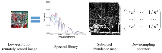
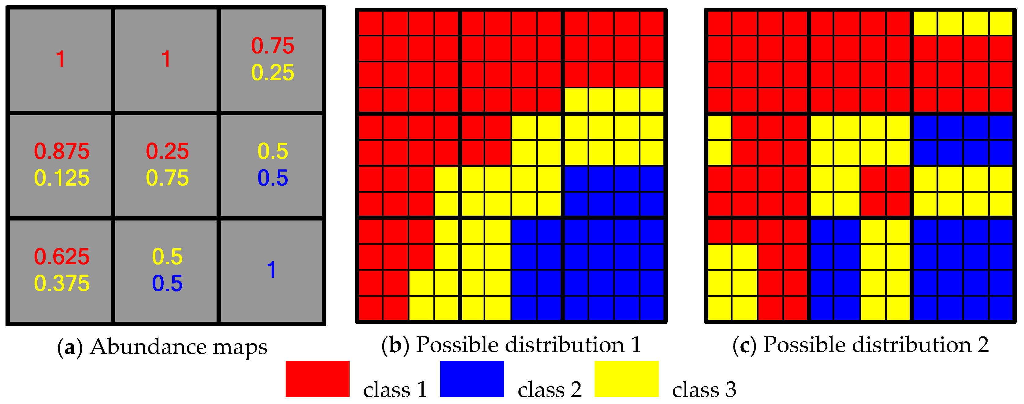
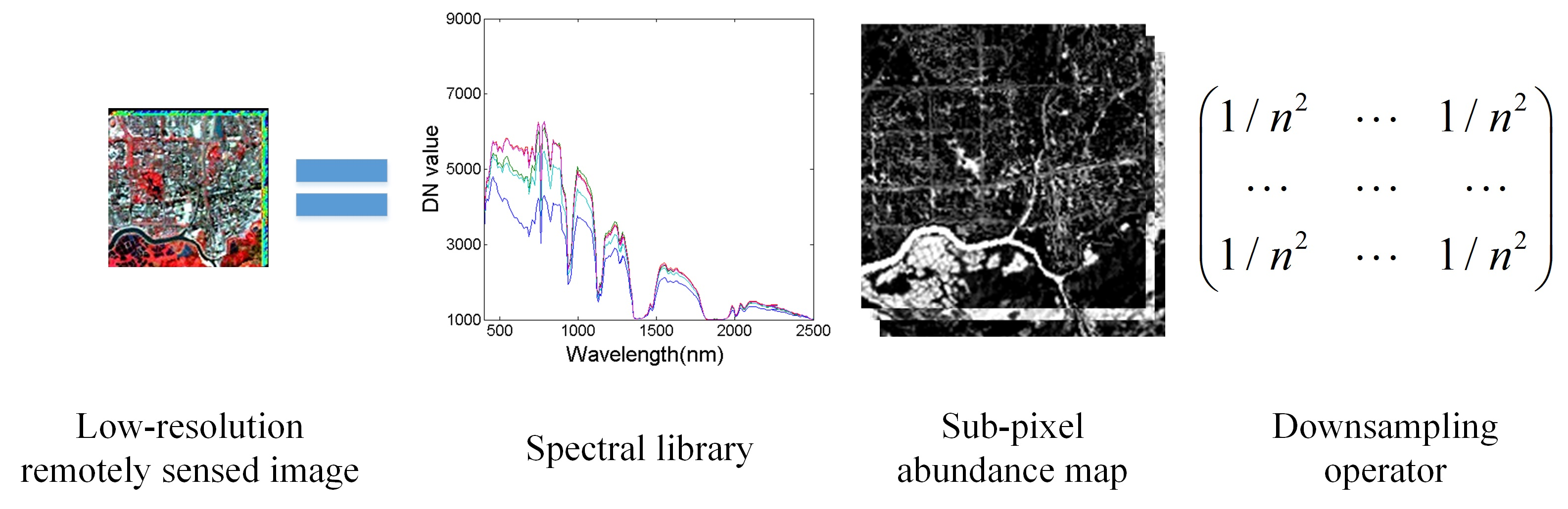
2. Sub-Pixel Mapping Problem

The key issue in a sub-pixel mapping problem is how to determine an optimal sub-pixel distribution of each class within a pixel. Spatial dependence has been regarded as a criterion that is related to the tendency of spatially close observations to be more alike than more distant observations [3]. As illustrated in Figure 1, given an abundance map obtained by spectral unmixing techniques, each coarse pixel can be divided into s × s sub-pixels, where s represents the scale factor. The number of sub-pixels for each land-cover class can be then determined by the fractional values of different classes. Figure 1 shows a sub-pixel mapping example with three classes. As shown in Figure 1a, a coarse pixel is divided into 16 (4 × 4) sub-pixels, where the scale fraction s equals 4, and 0.5 in the fraction image in red, which means that 8 (16 × 0.5) sub-pixels belong to land-cover class 1. Figure 1b,c describe two possible distributions of sub-pixels. Given the principle of spatial dependence, the former is perceived to be more optimal.

3. The Proposed Joint Sparse Subpixel Mapping Model

3.1. Basic JSSM Model

First of all, we define the formulations and notations used in this paper. Let Y = [ y 1 , , y n ] b × n be the observed remotely sensed image with b spectral bands and n pixels, let M = [ m 1 , , m p ] b × p collect the spectral signatures of p endmembers (p equals to the number of land cover classes if the endmember variability is not considered) present in Y , let A = [ a 1 , , a n ] p × n stand for the abundance maps associating with Y and M . Following the linear mixture model, we have
Y = M A + N s . t . :   A 0 ,   1 p T A = 1 n T
where N b × n is the noise in the data, A 0 and 1 p T A = 1 n T are the so called nonnegative and sum-to-one constraints, 1 p T = [ 1 , 1 , , 1 ] T is a column vector of size p of 1s. Commonly, the endmember spectra are collected from the observed remotely sensed image manually or determined by endmember extraction methods such as vertex component analysis (VCA) [40] and N-FINDR [41].
Let Z = [ Z 1 , , Z v ] p × v be the sub-pixel abundance map, where v = n × s 2 is the number of sub-pixels in, Z and s is the scaling factor. An explicit relationship between the abundance maps and the introduced sub-pixel abundance map can be established by resorting to a downsampling matrix as follows:
A = Z W ,
where W = [ d 1 , , d n ] v × n is the downsampling matrix, which can be constructed as
W = ( I l 1 s T ) T ( I r 1 s T ) T s 2 ,
where l and r are the number of lines and columns in Y , respectively, and the total number of samples in the observed image Y is n = l × r . In (3), denotes the Kronecker operator, I is an identity matrix with suitable dimension.
Then a joint model can be generated by combining (1) and (2):
Y = M Z W + N s . t . :   Z 0 ,   1 p T Z = 1 v T
where Z 0 and 1 p T Z = 1 v T , similar to those in (1), are the nonnegative and sum-to-one constraints, respectively. In this way, we can directly associate the final sub-pixel abundance map Z with the coarser image Y , along with the constraints.
As mentioned before, it is essential to take the endmember variability into consideration for the joint sub-pixel mapping model. In this paper, the popular sparse representation theory was utilized. The idea of sparse representation was firstly introduced for spectral unmixing of hyperspectral images considering that pure signatures may not present in the input data [42,43]. It assumes that mixed pixels can be expressed in the form of linear combinations of a number of pure spectral signatures known in advance and available in a library. In this proposed JSSM model, a number of endmember spectra are selected from the remotely sensed images manually for each land cover class to represent the endmember variability and an endmember library can therefore be generated. Then the fixed endmember matrix M = [ m 1 , , m p ] b × p in (4) is replaced by the spectral library D = [ d 1 , d q ] b × q as (5) shows. Specifically, q = i = 1 p q i is the number of endmember spectra in the library in which p is the observed number of land cover classes and q i is the number of collected spectra for certain class i.
Y = D Z W + N
Due to the small number of endmembers contributing to a mixed pixel, Z q × v is extremely sparse due to most of the lines being full of zeros. This sparse problem for the hyperspectral image can therefore be written as:
min Z Z 0   s . t .   Y D Z W F 2 δ
where Z 0 denotes the number of nonzero components of Z and δ 0 is the tolerated error derived from the noise or the model itself. Commonly the L 0 term can be replaced by the L 1 norm and this problem can be restated as follows [44,45]:
min Z Z 1   s . t .   Y D Z W F 2 δ
where Z 1 = | Z i , j | and the above constraint optimization problem can be converted into an unconstrained version by minimizing the respective Lagrangian function:
min Z 1 2 Y D Z W F 2 + λ Z 1 + τ R + ( Z )
where the parameter λ is a non-negative parameter which controls the relative weight of the sparsity of the solution and the term τ R + ( Z ) is the non-negative constraint. Moreover, the sum-to-one constraint is not considered as suggested by [42,43,46,47]. The term τ R + ( Z ) is defined in the set R + and obeys rules such as τ R + ( Z ) = 0 when Z R + , otherwise τ R + ( Z ) = + .

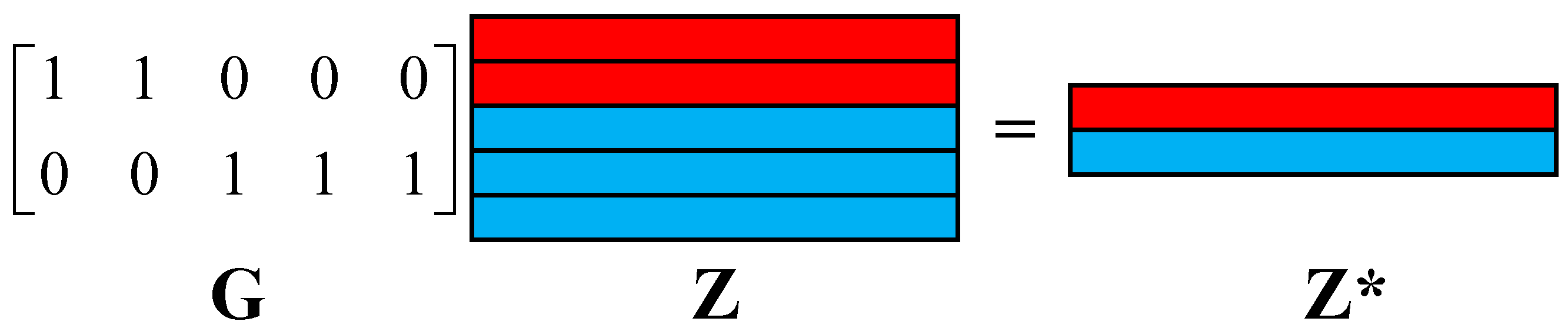
3.2. Spatial Prior Constraint

Owing to the ill-posed nature of the sub-pixel mapping problem which aims to generate a fine map from the coarser image, a spatial prior constraint is further imposed to regularize the problem. In this paper, the anisotropic TV model [48] is utilized by promoting piecewise smooth transitions in the sub-pixel abundance map. Moreover, it would be more suitable to conduct this operator on the class domain and not the endmember domain considering its physical interpretation as Figure 2 shows. It can be seen that the sub-pixel abundance map for all endmembers in the library should be first grouped according to the categories of endmembers for different classes.
Then the utilized TV operator can be imposed on Z* as (9).
T V ( Z* ) = x Z* 1 + y Z* 1 ,
where x and y are linear operators denoting the horizontal and vertical first-order differences. It is obvious that only the two directions are taken into consideration to represent the spatial dependence. For pixel i of class k in image Z*, its two-dimensional position can be indicated as (m, u) in which i = m × n × s + u and i v . Then each elements in x Z* and y Z* can be computed as Z k , i x = Z k [ m + 1 , u ] Z k [ m , u ] and Z k , i y = Z k [ m , u + 1 ] Z k [ m , u ] , respectively, where m = f l o o r ( i / ( n × s ) ) and u = i m × n × s . By combing the two linear operators, this TV model can be defined as:
T V ( Z* ) = x Z* y Z* 1 = Z* 1 = G Z 1

3.3. Optimization

With these definitions, this optimization problem can be rewritten as
min Z 1 2 Y D Z W F 2 + λ T V G Z 1 + λ Z 1 + τ R + ( Z )
where λ T V is the regularization parameter for the TV term. To solve this problem, the widely used alternating direction method of multipliers [43,49] is employed to decompose (11) into a sequence of simpler ones. By introducing auxiliary variables, the following constrained problem can be obtained.
min Z , V 1 , V 2 , V 3 , V 4 , V 5 , V 6 1 2 Y D V 2 F 2 + λ T V V 4 1 + λ V 5 1 + τ R + ( V 6 ) , s u b j e c t   t o V 1 = Z V 2 = V 1 W V 3 = G Z V 4 = V 3 V 5 = Z V 6 = Z
The expanded augmented Lagrangian formula is then obtained in (13) by adding the many ancillary terms that utilize the ADMM in the optimization problem (12).
J ( Z , V 1 , V 2 , V 3 , V 4 , V 5 , V 6 , S 1 , S 2 , S 3 , S 4 , S 5 , S 6 ) = 1 2 Y D V 2 F 2 + λ T V V 4 1 , 1 + λ V 5 1 , 1 + τ R + ( V 6 ) + μ 2 ( Z V 1 S 1 F 2 + V 1 W V 2 S 2 F 2 + G Z V 3 S 3 F 2 + V 3 V 4 S 4 F 2 + Z V 5 S 5 F 2 + Z V 6 S 6 F 2 )
where μ is the penalty parameter. In the following part, we elaborate on how to split the complicated optimization relation (13) based on the ADMM strategy, and give details of the derivation of the JSSM.
To achieve the solution Z of the augmented Lagrangian formula by performing an alternating minimization process, the partial derivative of (13) can be written as:
Z k + 1 min Z   J ( Z , V 1 k , V 2 k , V 3 k , V 4 k , V 5 k , V 6 k , S 1 k , S 2 k , S 3 k , S 4 k , S 5 k , S 6 k ) Z k + 1 ( G T G + 3 I ) 1 * { ( V 1 k + S 1 k ) + G T ( V 3 k + S 3 k ) + ( V 5 k + S 5 k ) + ( V 6 k + S 6 k ) }
The optimization of V i can be computed as follows, which is obtained by means of derivation. First, we compute the optimization of V 1 k + 1 as follows:
V 1 k + 1 { ( Z k + 1 S 1 k ) + ( V 2 k + S 2 k ) W T } ( I + W W T ) 1
Similarly, the optimization of V 2 k + 1 and V 3 k + 1 can be written as (16) and (17).
V 2 k + 1 ( D T D + μ I ) 1 ( D T Y + μ ( V 1 k + 1 W S 2 k ) )
V 3 k + 1 ( T + I ) 1 ( G Z k + 1 S 3 k + T ( V 4 k + S 4 k ) )
Here, is a convolution operator and it can be computed using the discrete Fourier transform diagonalization band by band as in [43]. Moreover, as the L 1 norm is not differentiable, in the case of L 1 sparse approximation of V 4 and V 5 , the solution is obtained by a soft shrinkage operator, as follows:
V 4 k + 1 s o f t ( V 3 k + 1 S 4 k , λ T V μ )
V 5 k + 1 s o f t ( Z k + 1 S 5 k , λ μ )
According to the definition of τ R + , the optimization of V 6 can be:
V 6 k + 1 max ( Z k + 1 S 6 k , 0 )
Finally, the Lagrangian multipliers are updated:
S 1 k + 1 S 1 k Z k + 1 + V 1 k + 1 S 2 k + 1 S 2 k V 1 k + 1 W + V 2 k + 1 S 3 k + 1 S 3 k G Z k + 1 + V 3 k + 1 S 4 k + 1 S 4 k V 3 k + 1 + V 4 k + 1 S 5 k + 1 S 5 k Z k + 1 + V 5 k + 1 S 6 k + 1 S 6 k Z k + 1 + V 6 k + 1
In summary, the ADMM strategy can be utilized as indicated in Equations (14)–(21) iteratively until a given number of iterations or a tolerance value of adjacent results is achieved. Moreover, the ADMM method is initialized as Z 0 = V i 0 = S i 0 = 0 ,   i [ 1 , 6 ] and the maximum iterative time is set as 200 in case the given stop threshold cannot be satisfied.
As a result, the sub-pixel abundance map Z can be obtained and it should be further grouped as Figure 1 shows to obtain the sub-pixel abundance map Z* in class domain where the value Z k , i * in Z* denotes the proportion of pixel i belonging to class k. Then the sub-pixel mapping result O with p classes can be expressed as O = f ( Z* ) , which means that it can be generated with the sub-pixel abundance map Z*, and different functions f ( ) can be used to convert the abundance map to a final sub-pixel mapping result. In this paper, a simple winner-takes-all strategy was designed to generate the final sub-pixel mapping result O as follows,
O i = j   i f   Z j , i * = max { Z k , i * | k ( 1 , p ) }

4. Experiments and Analysis

The proposed JSSM has been compared with three traditional sub-pixel mapping algorithms, including the attraction model (AM) [10], Hopfield neural network (HNN) [8], and MRF [24], in which AM and HNN are based on an obtained abundance map while the MRF can be conducted on the original remotely sensed image directly. Additionally, the abundance fractions in the abundance map act as a mandatory constraint for the sub-pixel mapping result generated by the AM method, while for HNN, a soft constraint strategy is utilized which means the final sub-pixel mapping result does not need to satisfy the abundance fraction constraint. Moreover, the abundance map can also be classified and further rescaled to generate a finer classification map which was also used to compare with the proposed JSSM method and this strategy is named as the hard classification (HC) method. Additionally, two spectral unmixing methods, FCLS [50] and SUnSAL-TV [43], were employed to generate the abundance maps for AM, HC, and HNN. Moreover, the endmember library used in the JSSM method was also applied for SUnSAL-TV while for FCLS, only one representative spectrum was determined for each endmember. Owing to the fact that the spectral curves of the identical land cover class vary greatly and it is hard to determine a most representative endmember for each class, the average spectral signature for each class is generate as the input of FCLS. For the utilized HNN method, the parameters were set as follows: λ is 100, k1 = k2 = k3 = 1, dt = 0.01. Moreover, different parameters were tested for SUnSAL-TV and the abundance map, with the highest accuracy on comparing with the reference abundance map, was selected as the one used for the following sub-pixel mapping procedure. In the proposed JSSM method, three parameters were taken into consideration as mentioned above: the spatial constraint parameter λ T V , the sparsity constraint parameter λ , and the penalty parameter μ .
In our experiments, three synthetic and one real hyperspectral images were used to evaluate the proposed JSSM method in comparison to other techniques. For the synthetic image experiments, an original high-resolution remotely sensed image was firstly degraded to obtain a low-resolution image by applying an averaging filter. The low-resolution image was then used to obtain different sub-pixel mapping results with spectral unmixing and sub-pixel mapping techniques. The high-resolution remotely sensed image can be classified to generate a reference classification map to evaluate different sub-pixel mapping methods. For the real experiment, spectral unmixing and sub-pixel mapping algorithms were applied on the low resolution hyperspectral image and the classification result of a high resolution image, which covers an identical area to the low resolution one, was used as the reference map.
Our accuracy assessment was undertaken using the overall (OA), average (AA) and individual classification (IA) accuracies, as well as the Kappa coefficient. Moreover, the root-mean-square error (RMSE) index was also utilized to evaluate the generated abundance results with two different spectral unmixing techniques by comparing with the reference abundance map which was generated from the reference classification map.
In addition, to test the statistical significance of the differences in accuracy for results of the proposed method and other algorithms, the McNemar’s test [51] was used to compare the misclassification rates with the different methods. For the two classification maps C 1 and C 2 , the McNemar’s test compares the number of pixels misclassified in C 1 , but not in C 2 ( M 12 ), with the number of pixels misclassified in C 2 while not in C 1 ( M 21 ). If M 12 + M 21 20 , the X 2 can be considered as a chi-squared distribution (with one degree of freedom) [52], [53] as (23):
X 2 = ( | M 12 M 21 | 1 ) 2 M 12 + M 21 χ 1 2
The McNemar’s test accepts the hypothesis that the two classification methods have the same error rate at significance level ε if the value is less than or equal to χ ε , 1 2 [54]. In other words, if the McNemar’s value is greater than χ ε , 1 2 , the two classification algorithms are significantly different. In this paper, the significance level ε is set as 0.05, which means χ ε , 1 2 = 3.84 .
The remainder of this section is organized as follows. First, we provide an evaluation of the accuracy achieved by the proposed approach (in comparison to other sub-pixel mapping approaches) using synthetic data. Then we provide an assessment and comparison using real hyperspectral scenes. The last section concludes with an evaluation of the impact of parameter settings on the newly developed JSSM approach.

4.1. Synthetic Experiments

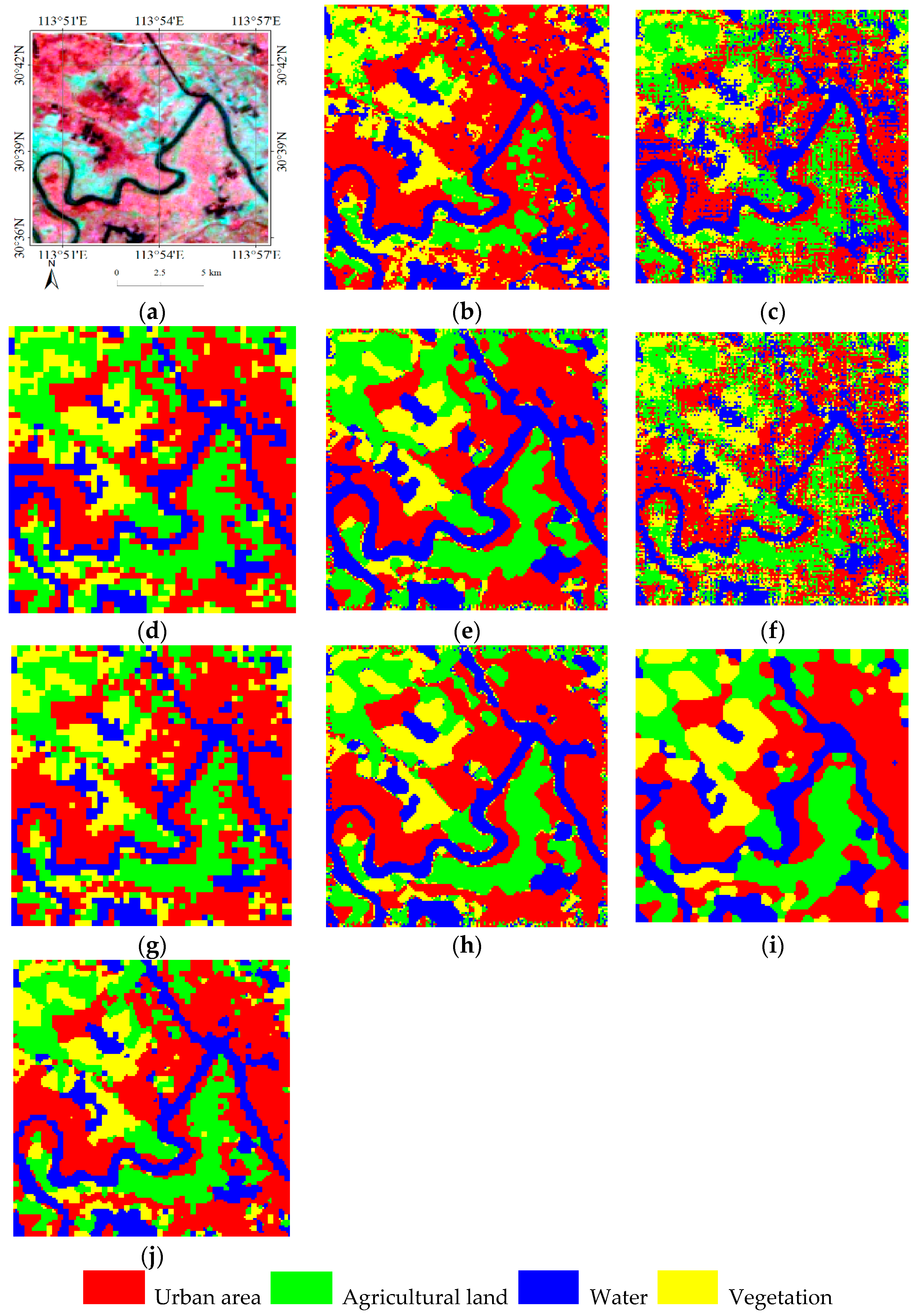
4.1.1. Synthetic Image 1: HJ-1A

To simulate a real world situation under a fully controlled scenario, we used a real hyperspectral data set which was obtained by a Chinese environmental satellite, HJ-1A [55]. The HJ-1A satellite has a hyperspectral sensor with 115 spectral bands (in the spectral range from 0.45 to 0.95 μm) and spatial resolution of 100 m per pixel. The utilized HJ-1A image (150 × 150 pixels) was acquired on 19 August 2009 and was used as the original image in our experiments. The study site is located in Hanchuan City, Hubei Province, central China, and its surrounding area. Four land-cover classes, i.e., urban, agricultural land, water, and vegetation are used to characterize this image as Figure 3b shows. This image was degraded artificially to obtain a low-resolution synthetic image given a scale factor of three in this experiment.
As illustrated in Figure 3, the abundance map used as initial condition can severely impact the final sub-pixel mapping results. Because of this, it can be observed for the FCLS based sub-pixel mapping results that there are small pepper and salt patches existing for the whole image. For the HNN, MRF, and JSSM in which the abundance fractions can be altered, better results can be obtained. It still can be observed that many algorithms can generate similar results. Like results of HNN and MRF, our method can also eliminate some details due to model error and excessive smoothing. There is a trade-off between smoothing and detail preservation, in the sense that smoothing can restrain the model error while potentially eliminating small features. However, this kind of trade-off is inevitable owing to the nature of sub-pixel mapping, which aims to generate a finer classification map from the low-resolution remotely sensed image.
Table 1 shows a quantitative comparison of the AM, HC, HNN, MRF and the proposed JSSM methods. It is obvious that the sub-pixel mapping results of traditional methods are greatly affected by the spectral unmixing errors. It should be noted that the relationship between the accuracies of spectral unmixing and sub-pixel mapping is not monotonic as expected by many researches if the abundance fractions acts as a constraint. Although SUnSAL-TV can generate a better abundance map (RMSE value is 0.180) than that of FCLS, the sub-pixel mapping results exhibit worst performance when the AM method is utilized. Therefore, it is reasonable to develop sub-pixel mapping algorithms, which are conducted on the original remotely sensed image, such as MRF and JSSM. It can be seen that the proposed JSSM shows an improvement when compared with the traditional sub-pixel mapping methods, regardless of which spectral unmixing methods are utilized to generate the abundance map. When compared with the MRF, a slight improvement can also be observed in all quantitative indexes. For example, a gain of 0.91% in AA is obtained for the proposed method from the MRF method. Moreover, the McNemar’s test is a useful tool for determining if two classification methods have significantly different prediction rates. From Table 1, it can be seen that most of the values of the McNemar’s test, except MRF, are greater than the critical value (3.84). This implies that the proposed method has significantly different prediction rates compared with most traditional algorithms. Generally, the proposed JSSM can exhibit better performance by considering the endmember variability in sub-pixel mapping for a remotely sensed image.

4.1.2. Synthetic Image 2: Flightline C1 (FLC1)

In this section, we use an aerial data set with agricultural crop species and land use (the band number is 12) by an optical mechanical line scanner referred to as the University of Michigan M-7 system. The flightline used in this experiment (called FLC1) was collected on 28 June 1966 [56]. It was taken over the southern part of Tippecanoe County of Indiana. The size in pixels of the image is 80 × 160 pixels and the low-resolution image was generated using a resize factor of four as Figure 4a shows. Then a classification result was obtained for FLC1 by classifying the original high-resolution image with the commercial eCognition software. A total of eight land cover classes can be distinguished in Figure 4b–h give the sub-pixel mapping results.
As illustrated in Figure 4, it is obvious that the impact of the abundance map is quite important for the subsequent sub-pixel mapping procedure for traditional methods. As most land classes are kinds of agricultural crop species, it is easier to observe higher between-class similarity and the within-class dispersion. Therefore, the sub-pixel mapping results would be more susceptible to endmember variability. It can be seen that many pixels are misclassified by the MRF in which the endmember variability is not considered and the proposed JSSM method performs better. Moreover, owing to the special characteristic of the FLC1 dataset that contains few tiny features, the JSSM method can generate an acceptable visual result by imposing spatial regularization.
Table 2 shows a quantitative comparison of the AM, HC, HNN, MRF and the proposed JSSM methods. Different from the HJ-1A dataset mentioned above, it should be noted that SUnSAL-TV based sub-pixel mapping results show a better performance than that of FCLS here with a lower RMSE for the abundance map. From the quantitative results of HJ-1A and FLC1 datasets, the conclusion can therefore be drawn that the abundance map with higher accuracy cannot assure a better sub-pixel mapping result if the abundance fractions acts as the constraint. By incorporating this rich information in the original remotely sensed image, a great improvement in quantitative statistics can be observed for JSSM. The quantitative indexes lead to the same conclusion as the visual assessment for JSSM compared with MRF and the proposed JSSM exhibits better accuracies for AA, OA, and Kappa indexes. The OA increases from 85.54% to 92.39% for the JSSM compared with the MRF which results from the consideration of endmember variability. The McNemar’s test also demonstrates that JSSM gives significant different results compared to the critical value (3.84). Therefore, it can be concluded that the proposed JSSM performs better than other sub-pixel mapping methods from visual and quantitative assessments.

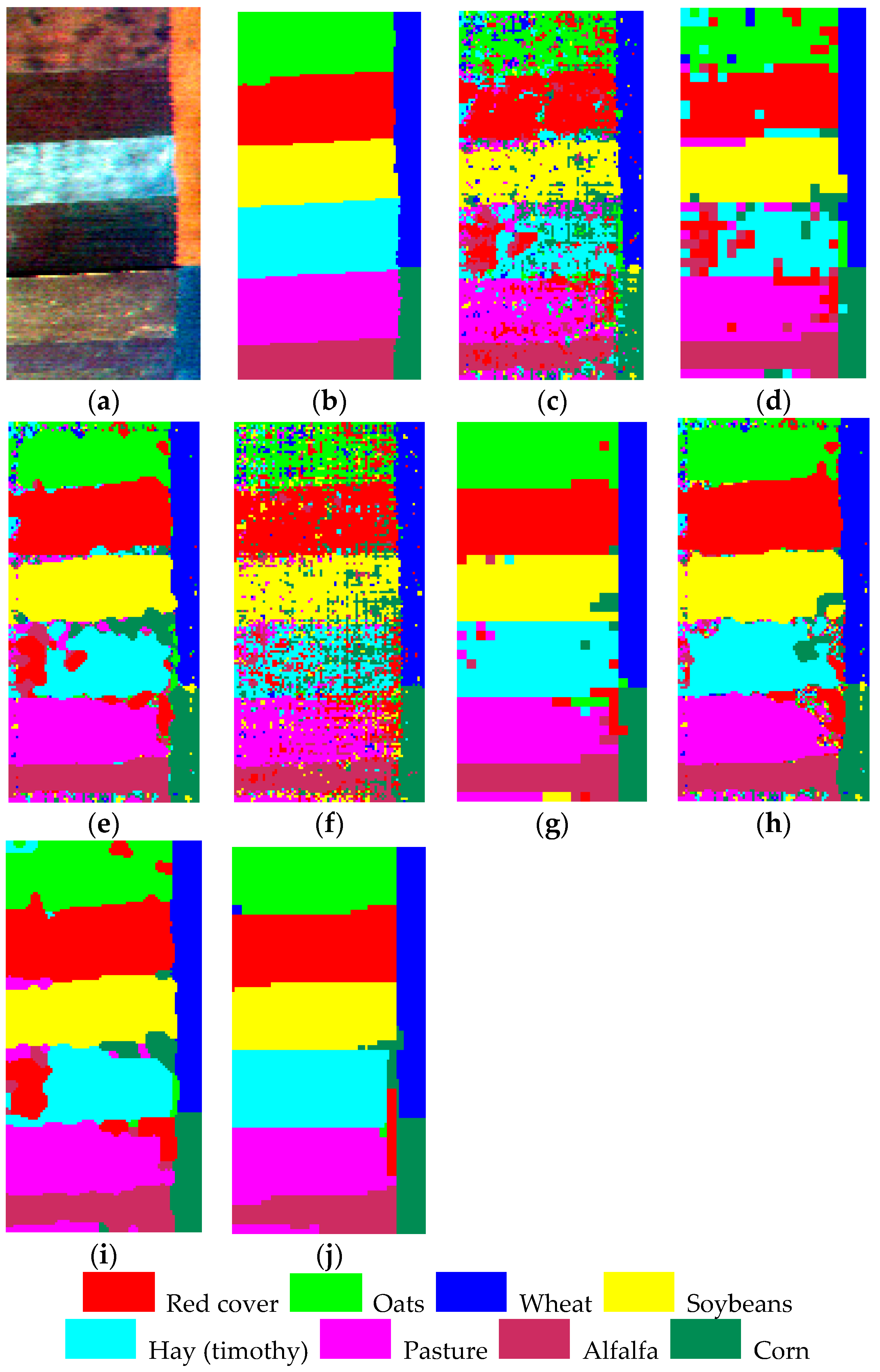
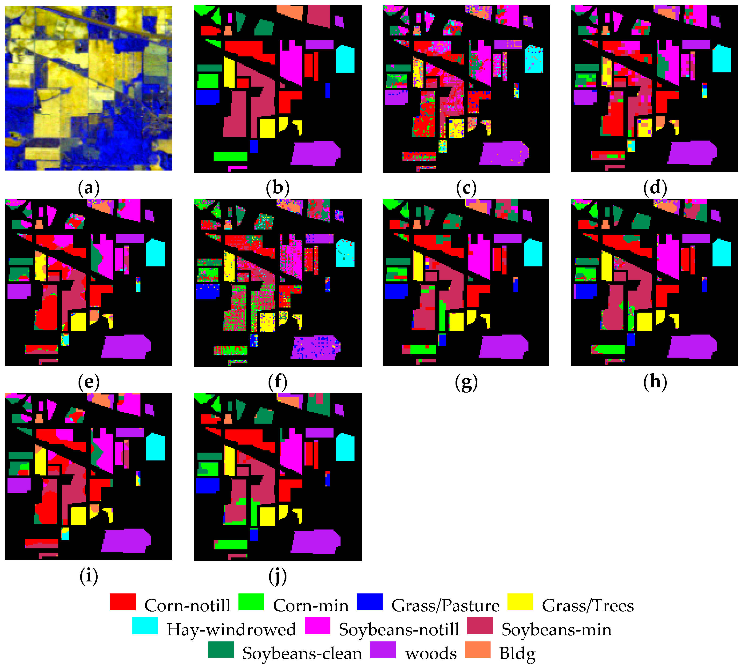
4.1.3. Synthetic Image 3: AVIRIS Indian Pines

The third image used in experiments is the commonly used AVIRIS Indian Pines dataset. Ten land cover classes were considered for classification. The utilized image is composed of 144 × 144 pixels and 220 bands, the ground truth data is also provided as the reference. The scale factor was set as three and Figure 5a shows the degraded AVIRIS hyperspectral image cube; Figure 5b shows the ground truth data in which 10 major land-cover classes can be distinguished and Figure 5c–h illustrate the sub-pixel mapping results with different algorithms.
The utilized Indian Pines image is well known for its land cover class spectral variability and severe noises in fields such as image classification and denoising. Therefore, the utilization of the endmember library can play an important role in the sub-pixel mapping procedure. For the Indian Pines image, the same conclusions can be drawn as for the previous two datasets. For the abundance map based sub-pixel mapping results, many isolated small false features can be found owing to the errors in the abundance map. While for the JSSM methods, these kinds of errors can be mitigated. Compared with the reference map, it can be seen that the proposed JSSM method can exhibit better performance by incorporating various endmember spectra of land cover classes than that of MRF. As shown in Figure 5, it can be distinguished that many patches of class Soybeans-clean are badly contaminated by other classes as the result of MRF while in the JSSM result, more homogeneous areas can be observed.
The sub-pixel mapping accuracies obtained in this experiment are listed in Table 3 to evaluate the effectiveness of the proposed method in quantitative fashion. It can be seen that the SUnSAL-TV based results show a great improvement compared with FCLS based results for both the abundance map and sub-pixel maps owing to the consideration of class spectral variability. The SUnSAL-TV based methods can even exhibit comparable results to the JSSM method. Moreover, it is easy to notice the big gaps between the JSSM and MRF methods for all quantitative indexes. For example, the JSSM improves the Kappa coefficient from 0.496 to 0.825 when compared with MRF. Generally, a better result can be obtained with the proposed JSSM quantitatively, especially for those images suffering from severe conditions of endmember variability.

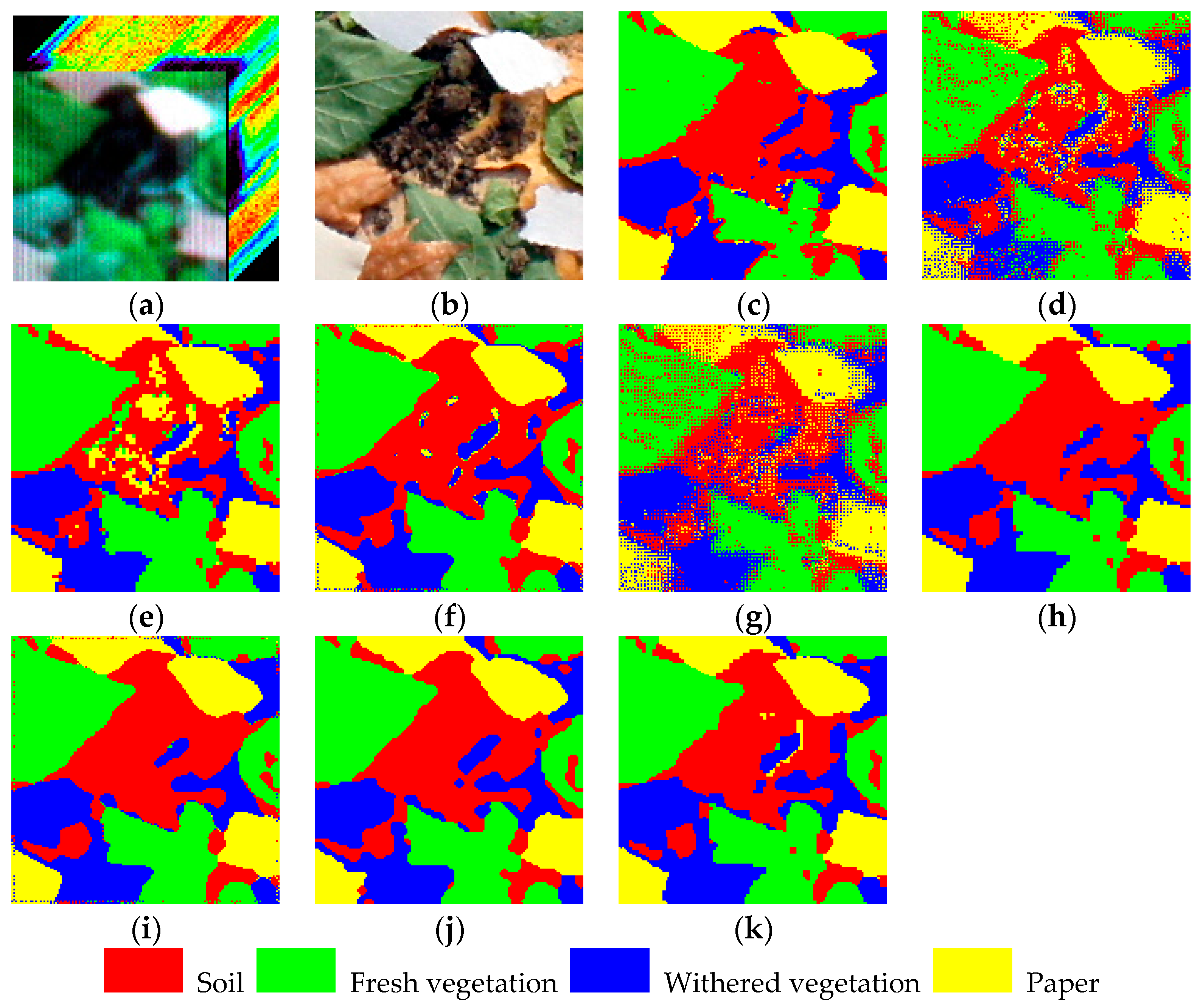
4.2. Real Experiment-Nuance Dataset

To evaluate the practical application of the proposed method, a real experiment was implemented by acquiring a real hyperspectral image and a higher resolution color image for the same area, simultaneously. The original (low resolution) hyperspectral image (80 × 80 pixels) was collected using the Nuance NIR imaging spectrometer. The acquired hyperspectral image has 46 bands, and the spectral range is from 650–1100 nm, with 10 nm spectral sampling interval. The higher resolution color image (160 × 160 pixels) was obtained by a digital camera for the same scene, and the considered scale factor was two. The reference classification map was obtained by classifying the high resolution color image using the SVM. Four major land-cover classes can be distinguished in this experiment: soil, fresh vegetation, withered vegetation, and white paper. Figure 6a–c illustrates the original hyperspectral image, the high resolution color image, and the high resolution classification map used as reference, respectively. Figure 6d–i shows the sub-pixel mapping results obtained using AM, HC, HNN, MRF, and the proposed JSSM approach, respectively.
As shown in Figure 6, it is obvious that the proposed method can provide a better visual result compared with FCLS based sub-pixel mapping algorithms. Moreover, it can be seen that the difference between the JSSM and some other results is not so distinct. It is because the utilized Nuance image was acquired with a ground based imaging spectrometer and therefore, the impact of atmospheric and illumination conditions on the spectral variability can be suppressed. However, it still can be distinguished from the Figure 6 that the proposed JSSM shows a better result in some regions such as the shape of the paper at the bottom left of this image.
The accuracies and statistics of the different methods are listed in Table 4. As illustrated in this table, the proposed JSSM also provides improvements in this experiment in terms of all indexes when compared with other sub-pixel mapping results. Although the MRF method can generate a comparable result with JSSM owing to the inconspicuous endmember variability for the Nuance dataset, the JSSM method still increases the AA from 86.64% to 87.49%, a gain of 0.85%, when compared with the MRF method. Moreover, the McNemar’s value indicates that JSSM gives a significantly different performance, compared to the other methods. Generally, both the visual assessment and quantitative accuracies indicate that JSSM performs better than the other sub-pixel mapping methods tested in this work.

4.3. Discussion

In the proposed JSSM method, three parameters were taken into consideration: the spatial constraint parameter λ T V , the sparsity constraint parameter λ and the penalty parameter μ . These parameters have a great impact on the objective criteria’s optimization, or are sensitive to different data and significantly influence the sub-pixel mapping accuracy. To ensure our conclusions can be generalized to datasets with different gray level ranges, all images considered in the experiments were normalized to the range 0–1. We let all parameters vary from 10−6 to 10−1 at a rate of 5 and Figure 7 and Figure 8 depict the impact of different values of parameters on the obtained accuracy for all considered experiments. Besides, the performance of the proposed JSSM method under different scale factors were also tested.

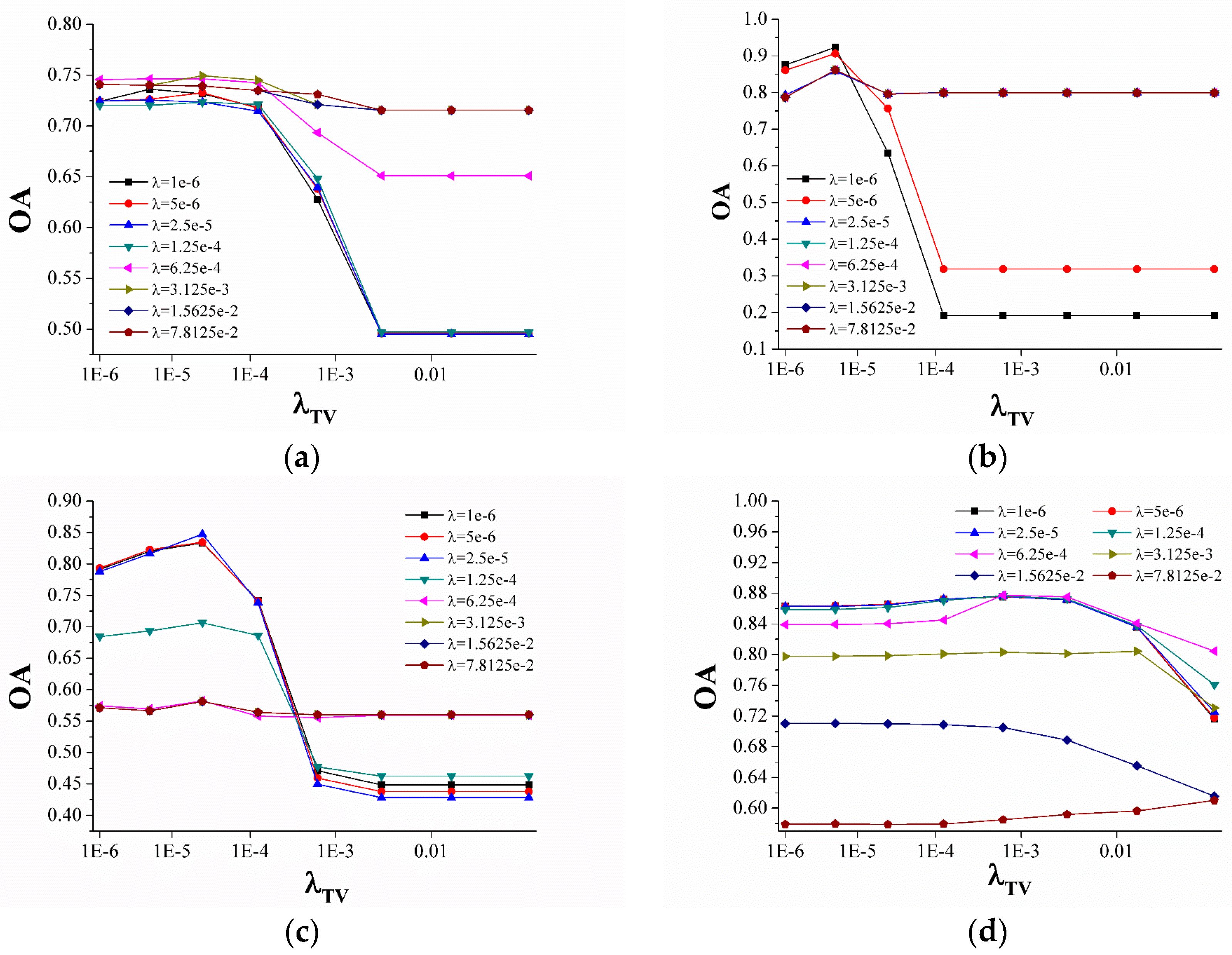
4.3.1. The Impact of the Penalty Parameter μ

To evaluate the impact of the penalty parameter μ , the highest accuracy of different μ values is obtained for all experimental datasets as Figure 7 shows. It can be seen that the trends for different datasets are not so consistent with each other. For the simulated FLC1 and Indian Pines images, the accuracy will decrease greatly since a certain threshold is satisfied. While for HJ-1A, the curve is more flat and a higher accuracy is further achieved with a greater value of μ for the Nuance dataset. However, acceptable results can be generated with a relative small value of μ for all datasets as shown in Figure 7. Therefore, the selection of the penalty parameter can be limited to around 10−3 empirically.

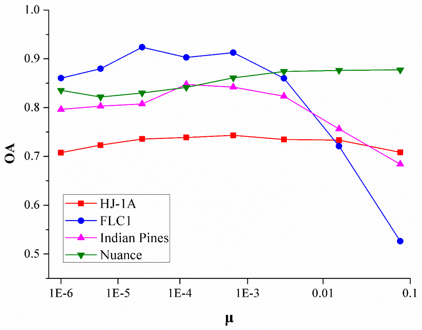
4.3.2. The Impact of the Regularization Parameter λ T V and λ

For the two regularization parameters, the optimal penalty parameter is determined firstly for different datasets. Figure 8 illustrates the accuracies of different parameters λ T V and λ with all datasets. A similar pattern can be observed for simulated experiments and some curves are overlapped. It is easy to realize the difference of curves with simulated and real datasets; however, the same conclusions can be obtained that relative small values of λ T V and λ can also give acceptable sub-pixel mapping results, while for the Indian Pines and Nuance datasets, a greater value of λ can make the accuracy decrease dramatically. Generally, the values of λ T V and λ can be set around 10−5 to ensure the generalization.

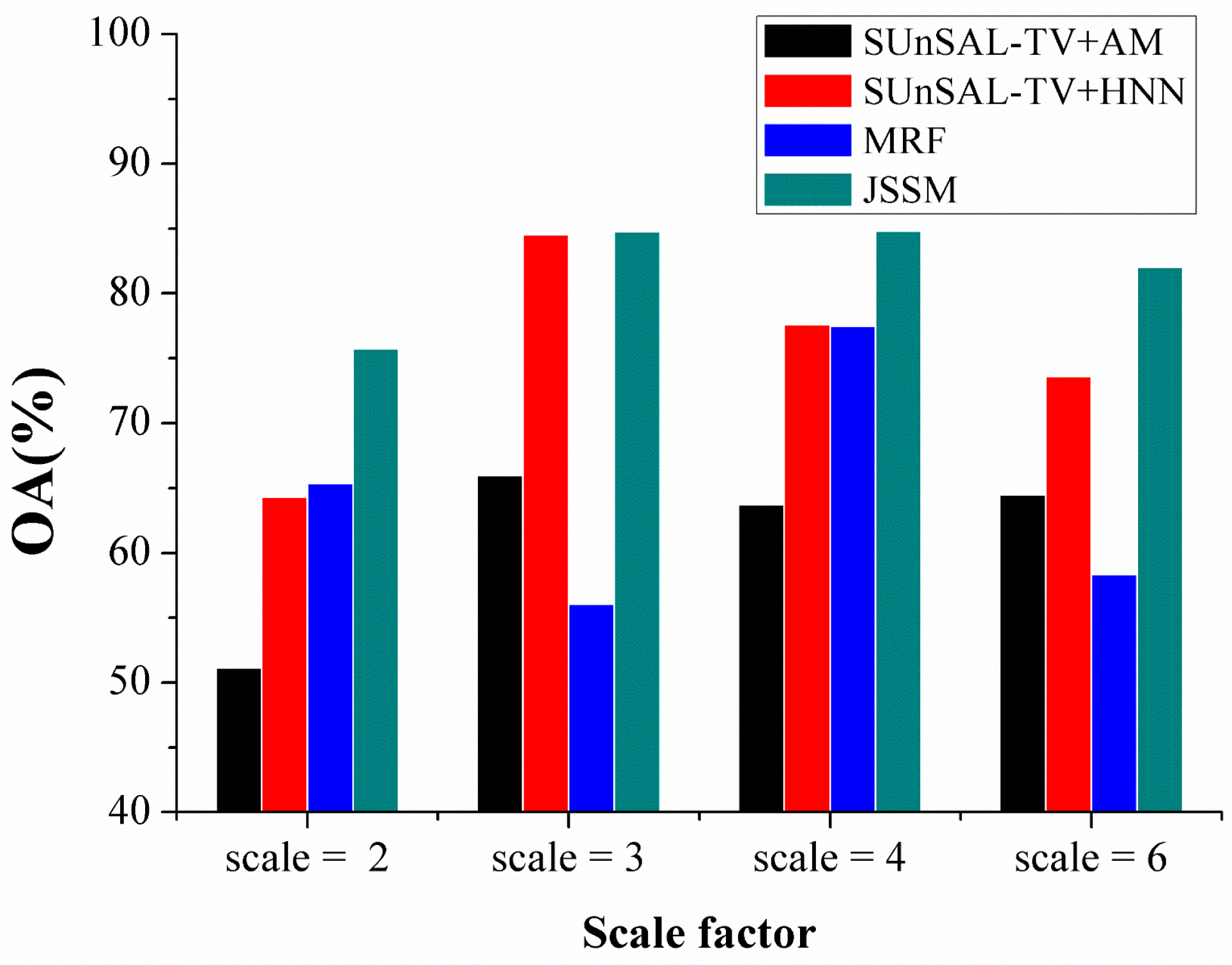
4.3.3. The Impact of Different Scale Factors

In the previous experiments, the scale factor was set as two, three, or four for different datasets. To illustrate the performance of the proposed JSSM under different scale factors, the simulated Indian Pines dataset was used to test different sub-pixel mapping algorithms. Figure 9 shows the accuracies of different methods when the scale factor is set as two, three, four, and six respectively. It is obvious that the proposed JSSM method generates the highest accuracies for different scale factors compared with other sub-pixel mapping methods. Moreover, it can also be found that the relationship between the accuracy of sub-pixel mapping and the scale factor is not monotonic. The sub-pixel mapping algorithms always achieve the highest accuracies when a moderate scale factor is given, such as three or four.

5. Conclusions and Future Lines

In this paper, we presented a new joint sparse sub-pixel mapping (JSSM) model for remotely sensed imagery. The proposed approach incorporates endmember variability into the sub-pixel mapping process by selecting variable representative spectra for each endmember in a library. Although the sub-pixel mapping is commonly regarded as the subsequent procedure of spectral unmixing, it is also shown in this paper that the use of a highly accurate abundance map does not always ensure a better sub-pixel mapping result. As a result, it is very important to address the problem of endmember variability for sub-pixel mapping on the original remotely sensed imagery directly, as opposed to traditional sub-pixel mapping algorithms which act on the abundance map. Compared with these traditional algorithms, which utilize a single spectrum for each endmember, the newly proposed JSSM can mitigate the impact of spectral variability and therefore provide a better sub-pixel mapping result. Our experimental results, conducted with a comprehensive database of synthetic and real images, indicate that JSSM is indeed an efficient sub-pixel mapping technique. Moreover, the proposed JSSM was also compared with its simplified version in which the endmember variability was not considered and the same conclusion can be drawn that the utilization of endmember variability improves the performance of sub-pixel mapping greatly. Although the proposed JSSM has been observed to outperform other traditional sub-pixel mapping methods, this model should be developed to incorporate additional datasets owing to the ill-posed nature of sub-pixel mapping. In this way, more robust and reliable sub-pixel mapping can be further generated. Additionally, it can also be seen in the experimental results that JSSM will give stairs (piecewise constant regions) owing to the utilization of the TV model. Our future work will focus on the extension of the proposed JSSM method for multi-temporal remotely sensed images in which the spectral variability is a severe problem owing to environmental, atmospheric, and temporal factors. Moreover, the automatic generation of the endmember library should be further taken into consideration and other spatial models, such as the non-local TV, will also be tested.

Acknowledgments

The work described in the paper was substantially supported by the China Postdoctoral Science Foundation (Project Nos. 2014M560353 and 2015T80450), the National Natural Science Foundation of China (Project Nos. 41401398, 41325005, 41201426, 41171352, 41171327, 41371344 and 41622107), the Fund of Shanghai Outstanding Academic Leaders Program (Project No. 12XD1404900), and the KwangHua Foundation of College of Civil Engineering, Tongji University.

Author Contributions

Xiong Xu, Xiaohua Tong and Antonio Plaza conceived and designed the experiments; Yanfei Zhong performed the experiments; Yanfei Zhong and Huan Xie analyzed the data; Xiaohua Tong and Liangpei Zhang contributed reagents/materials/analysis tools; Xiong Xu wrote the paper.

Conflicts of Interest

The authors declare no conflict of interest.

References

  1. Bioucas-Dias, J.M.; Plaza, A.; Camps-Valls, G.; Scheunders, P.; Nasrabadi, N.M.; Chanussot, J. Hyperspectral remote sensing data analysis and future challenges. IEEE Geosci. Remote Sens. Mag. 2013, 1, 6–36. [Google Scholar] [CrossRef]
  2. Bioucas-Dias, J.M.; Plaza, A.; Dobigeon, N.; Parente, M.; Du, Q.; Gader, P.; Chanussot, J. Hyperspectral unmixing overview: Geometrical, statistical, and sparse regression-based approaches. IEEE J. Sel. Top. Signal Process. 2012, 5, 354–379. [Google Scholar] [CrossRef]
  3. Atkinson, P.M. Mapping sub-pixel boundaries from remotely sensed images. In Innovations in GIS IV; Taylor and Francis: London, UK, 1997; Volume 12, pp. 166–180. [Google Scholar]
  4. Atkinson, P.M. Issues of uncertainty in super-resolution mapping and their implications for the design of an inter-comparison study. Int. J. Remote Sens. 2009, 30, 5293–5308. [Google Scholar] [CrossRef]
  5. Tobler, W.R. A computer movie simulating urban growth in the Detroit region. Econom. Geogr. 1970, 46, 234–240. [Google Scholar] [CrossRef]
  6. Atkinson, P.M. Sub-pixel target mapping from soft-classified, remotely sensed imagery. Photogramm. Eng. Remote Sens. 2005, 71, 839–846. [Google Scholar] [CrossRef]
  7. Su, Y.F.; Foody, G.M.; Muad, A.M.; Cheng, K.S. Combining pixel swapping and contouring methods to enhance super-resolution mapping. IEEE J. Sel. Top. Appl. Earth Observ. Remote Sens. 2012, 5, 1428–1437. [Google Scholar]
  8. Tatem, A.J.; Lewis, H.G.; Atkinson, P.M.; Nixon, M.S. Super-resolution target identification from remotely sensed images using a Hopfield neural network. IEEE Trans. Geosci. Remote Sens. 2001, 39, 781–796. [Google Scholar] [CrossRef]
  9. Li, X.; Ling, F.; Du, Y.; Feng, Q.; Zhang, Y. A spatial–temporal Hopfield neural network approach for super-resolution land cover mapping with multi-temporal different resolution remotely sensed images. ISPRS J. Photogramm. Remote Sens. 2014, 93, 76–87. [Google Scholar] [CrossRef]
  10. Mertens, K.C.; Baets, B.D.; Verbeke, L.P.C.; Wulf, R.R.D. A sub-pixel mapping algorithm based on sub-pixel/pixel spatial attraction models. Int. J. Remote Sens. 2006, 27, 3293–3310. [Google Scholar] [CrossRef]
  11. Tong, X.; Zhang, X.; Shan, J.; Xie, H.; Liu, M. Attraction-repulsion model-based subpixel mapping of multi-/hyperspectral imagery. IEEE Trans. Geosci. Remote Sens. 2013, 51, 2799–2814. [Google Scholar] [CrossRef]
  12. Xu, X.; Zhong, Y.; Zhang, L. A sub-pixel mapping method based on an attraction model for multiple shifted remotely sensed images. Neurocomputing 2014, 134, 79–91. [Google Scholar] [CrossRef]
  13. Mertens, K.C.; Verbeke, L.P.C.; Ducheyne, E.I.; Wulf, R.R.D. Using genetic algorithms in sub-pixel mapping. Int. J. Remote Sens. 2003, 24, 4241–4247. [Google Scholar] [CrossRef]
  14. Li, L.; Chen, Y.; Xu, T.; Liu, R.; Shi, K.; Huang, C. Super-resolution mapping of wetland inundation from remote sensing imagery based on integration of back-propagation neural network and genetic algorithm. Remote Sens. Environ. 2015, 164, 142–154. [Google Scholar] [CrossRef]
  15. Xu, X.; Zhong, Y.; Zhang, L. Adaptive sub-pixel mapping based on a multi-agent system for remote sensing imagery. IEEE Trans. Geosci. Remote Sens. 2014, 52, 787–804. [Google Scholar] [CrossRef]
  16. Xu, X.; Zhong, Y.; Zhang, L.; Zhang, H. Sub-pixel mapping based on a MAP model with multiple shifted hyperspectral imagery. IEEE J. Sel. Top. Appl. Earth Observ. Remote Sens. 2013, 6, 580–593. [Google Scholar] [CrossRef]
  17. Zhong, Y.; Wu, Y.; Zhang, L.; Xu, X. Adaptive MAP sub-pixel mapping model based on regularization curve for multiple shifted hyperspectral imagery. ISPRS J. Photogramm. Remote Sens. 2014, 96, 134–148. [Google Scholar] [CrossRef]
  18. Zhong, Y.; Wu, Y.; Xu, X.; Zhang, L. An adaptive subpixel mapping method based on MAP model and class determination strategy for hyperspectral remote sensing imagery. IEEE Trans. Geosci. Remote Sens. 2015, 53, 1411–1426. [Google Scholar] [CrossRef]
  19. Zhong, Y.; Zhang, L. Remote sensing image sub-pixel mapping based on adaptive differential evolution. IEEE Trans. Syst. Man Cybern. B Cybern. 2012, 42, 1306–1329. [Google Scholar] [CrossRef] [PubMed]
  20. Wang, Q.; Shi, W. Utilizing multiple subpixel shifted images in subpixel mapping with image interpolation. IEEE Geosci. Remote Sens. Lett. 2013, 11, 798–802. [Google Scholar] [CrossRef]
  21. Wang, Q.; Shi, W.; Atkinson, P.M. Sub-pixel mapping of remote sensing images based on radial basis function interpolation. ISPRS J. Photogramm. Remote Sens. 2014, 92, 1–15. [Google Scholar] [CrossRef]
  22. Ge, Y.; Chen, Y.; Li, S.; Jiang, Y. Vectorial boundary-based sub-pixel mapping method for remote-sensing imagery. Int. J. Remote Sens. 2015, 35, 1756–1768. [Google Scholar] [CrossRef]
  23. Ge, Y.; Li, S.; Lakhan, V.C. Development and testing of a subpixel mapping algorithm. IEEE Trans. Geosci. Remote Sens. 2009, 47, 2155–2164. [Google Scholar]
  24. Kasetkasem, T.; Arora, M.; Varshney, P. Super-resolution land cover mapping using a Markov random field based approach. Remote Sens. Environ. 2005, 96, 302–314. [Google Scholar] [CrossRef]
  25. Ling, F.; Fang, S.; Li, W.; Li, X.; Xiao, F.; Zhang, Y.; Du, Y. Post-processing of interpolation-based super-resolution mapping with morphological filtering and fraction refilling. Int. J. Remote Sens. 2014, 35, 5251–5262. [Google Scholar] [CrossRef]
  26. Li, X.; Ling, F.; Du, Y. Super-resolution mapping based on the supervised fuzzy c-means approach. Remote Sens. Lett. 2012, 3, 501–510. [Google Scholar] [CrossRef]
  27. Ling, F.; Du, Y.; Xiao, F.; Li, X. Subpixel land cover mapping by integrating spectral and spatial information of remotely sensed imagery. IEEE Geosci. Remote Sens. Lett. 2012, 9, 408–412. [Google Scholar] [CrossRef]
  28. Zhang, Y.; Du, Y.; Ling, F.; Wang, X.; Li, X. Spectral–spatial based sub-pixel mapping of remotely sensed imagery with multi-scale spatial dependence. Int. J. Remote Sens. 2015, 36, 2831–2850. [Google Scholar] [CrossRef]
  29. Chen, Y.; Ge, Y.; Jia, Y. Integrating object boundary in super-resolution land-cover mapping. IEEE J. Sel. Top. Appl. Earth Observ. Remote Sens. 2016. [Google Scholar] [CrossRef]
  30. Tong, X.; Xu, X.; Plaza, A.; Xie, H.; Pan, H.; Cao, W.; Lv, D. A new genetic method for subpixel mapping using hyperspectral images. IEEE J. Sel. Top. Appl. Earth Observ. Remote Sens. 2015, 9, 4480–4491. [Google Scholar] [CrossRef]
  31. Ling, F.; Du, Y.; Xiao, F.; Xue, H.; Wu, S. Super-resolution land-cover mapping using multiple sub-pixel shifted remotely sensed images. Int. J. Remote Sens. 2010, 31, 5023–5040. [Google Scholar] [CrossRef]
  32. Ling, F.; Li, X.; Xiao, F.; Fang, S.; Du, Y. Object-based sub-pixel mapping of buildings incorporating the prior shape information from remotely sensed imagery. J. Appl. Earth Obs. Geoinf. 2010, 18, 283–292. [Google Scholar] [CrossRef]
  33. Su, Y. Spatial continuity and self-similarity in super-resolution mapping: Self-similar pixel swapping. Remote Sens. Lett. 2016, 7, 338–347. [Google Scholar] [CrossRef]
  34. Somers, B.; Asner, G.; Tits, L.; Coppin, P. Endmember variability in spectral mixture analysis: A review. Remote Sens. Environ. 2011, 115, 1603–1616. [Google Scholar] [CrossRef]
  35. Zare, A.; Ho, K.C. Endmember variability in hyperspectral analysis. IEEE Signal Process. Mag. 2014, 31, 95–104. [Google Scholar] [CrossRef]
  36. Roberts, D.; Gardner, M.; Church, R.; Ustin, S.; Scheer, G.; Green, R.O. Mapping chaparral in the Santa Monica mountains using multiple endmember spectral mixture models. Remote Sens. Environ. 1998, 65, 267–279. [Google Scholar] [CrossRef]
  37. Bateson, C.A.; Asner, G.P.; Wessman, C.A. Endmember bundles: A new approach to incorporating endmember variability into spectral mixture analysis. IEEE Trans. Geosci. Remote Sens. 2000, 38, 1083–1093. [Google Scholar] [CrossRef]
  38. Castrodad, A.; Xing, Z.; Greer, J.; Bosch, E.; Carin, L.; Sapiro, G. Learning discriminative sparse representations for modeling, source separation, and mapping of hyperspectral imagery. IEEE Trans. Geosci. Remote Sens. 2011, 49, 4263–4281. [Google Scholar] [CrossRef]
  39. Zare, A.; Gader, P.; Dranishnikov, D.; Glenn, T. Spectral unmixing using the beta compositional model. In Proceedings of the IEEE Workshop on Hyperspectral Image and Signal Processing: Evolution in Remote Sensing, Gainesville, FL, USA, 25–28 June 2013.
  40. Nascimento, J.M.P.; Bioucas-Dias, J.M. Vertex component analysis: A fast algorithm to unmix hyperspectral data. IEEE Trans. Geosci. Remote Sens. 2005, 43, 898–910. [Google Scholar] [CrossRef]
  41. Winter, M. N-FINDR: An algorithm for fast autonomous spectral endmember determination in hyperspectral data. Proc. SPIE 1999, 3753, 266–277. [Google Scholar]
  42. Iordache, D.; Bioucas-Dias, J.M.; Plaza, A. Sparse unmixing of hyperspectral data. IEEE Trans. Geosci. Remote Sens. 2011, 49, 2014–2039. [Google Scholar] [CrossRef]
  43. Iordache, D.; Bioucas-Dias, J.M.; Plaza, A. Total variation spatial regularization for sparse hyperspectral unmixing. IEEE Trans. Geosci. Remote Sens. 2012, 50, 4484–4502. [Google Scholar] [CrossRef]
  44. Candès, E.; Tao, T. Decoding by linear programming. IEEE Trans. Inf. Theory 2005, 51, 4203–4215. [Google Scholar] [CrossRef]
  45. Candès, E.; Tao, T. Near-optimal signal recovery from random projections: Universal encoding strategies. IEEE Trans. Inf. Theory 2006, 52, 5406–5424. [Google Scholar] [CrossRef]
  46. Dópido, I.; Zortea, M.; Villa, A.; Plaza, A.; Gamba, P. Unmixing prior to supervised classification of remotely sensed hyperspectral images. IEEE Geosci. Remote Sens. Lett. 2011, 8, 760–764. [Google Scholar] [CrossRef]
  47. Dópido, I.; Villa, A.; Plaza, A.; Gamba, P. A quantitative and comparative assessment of unmixing-based feature extraction techniques for hyperspectral image classification. IEEE J. Sel. Top. Appl. Earth Observ. Remote Sens. 2012, 5, 421–435. [Google Scholar] [CrossRef]
  48. Ng, M.; Shen, H.; Lam, E.; Zhang, L. A total variation regularization based super resolution reconstruction algorithm for digital video. EURASIP J. Adv. Signal Process. 2007, 2007, 1–16. [Google Scholar] [CrossRef]
  49. Eckstein, J.; Bertsekas, D. On the Douglas-Rachford splitting method and the proximal point algorithm for maximal monotone operators. Math. Program. Ser. A/B 1992, 55, 293–318. [Google Scholar] [CrossRef]
  50. Heinz, D.C.; Chang, C.I. Fully constrained least square linear spectral unmixing analysis method for material quantification in hyperspectral imagery. IEEE Trans. Geosci. Remote Sens. 2001, 39, 529–545. [Google Scholar] [CrossRef]
  51. McNemar, Q. Note on the sampling error of the difference between correlated proportions or percentages. Psychometrika 1947, 12, 153–157. [Google Scholar] [CrossRef] [PubMed]
  52. Debeir, O.; Van den Steen, I.; Latinne, P.; Van Ham, P.; Wolff, E. Textural and contextual land-cover classification using single and multiple classifier systems. Photogramm. Eng. Remote Sens. 2002, 68, 597–606. [Google Scholar]
  53. Zhong, Y.; Zhang, L. An adaptive artificial immune network for supervised classification of multi-/hyperspectral remote sensing imagery. IEEE Trans. Geosci. Remote Sens. 2012, 50, 894–909. [Google Scholar] [CrossRef]
  54. Alpaydin, E. Introduction to Machine Learning; MIT Press: Cambridge, MA, USA, 2004. [Google Scholar]
  55. Bai, G. China environmental and disaster monitoring and forecasting small satellite—HJ-1A/B. Aerosp. China 2009, 5, 10–15. [Google Scholar]
  56. Hoffer, R.M. Computer-aided analysis of multispectral scanner data-the beginnings. In Proceedings of the ASPRS 2009 Annual Conference, Baltimore, MD, USA, 9–13 March 2009.
Figure 1. An example illustrating sub-pixel mapping methods. (a) Abundance maps are extracted for a 3 × 3-pixel image; (b) A possible distribution of sub-pixels in a finer resolution image in which a coarse pixel is divided into 16 (4 × 4) sub-pixels; (c) Another distribution perceived as less optimal than the one reported in (b).
Remotesensing 09 00015 g001
Figure 2. The class domain and the endmember domain for the sub-pixel abundance map. Z q × v is the sub-pixel abundance map in endmember domain with two classes (labelled as red and blue) and five endmember spectra and Z* p × v is the sub-pixel abundance map in the class domain with two classes. G p × q is a grouping matrix to transform Z into Z*.
Remotesensing 09 00015 g002
Figure 3. Sub-pixel mapping results for the synthetic dataset (HJ-1A): (a) original high-resolution remotely sensed imagery; (b) reference classification map obtained by SVM classifier; (c) sub-pixel mapping result obtained using FCLS+AM; (d) FCLS+HC; (e) FCLS+HNN; (f) SUnSAL-TV+AM; (g) SUnSAL-TV+HC; (h) SUnSAL-TV+HNN; (i) MRF; (j) JSSM.
Remotesensing 09 00015 g003
Figure 4. Sub-pixel mapping results for the synthetic dataset (FLC1): (a) original high-resolution remotely sensed imagery; (b) reference classification map obtained by eCognition software; (c) sub-pixel mapping result obtained using FCLS+AM; (d) FCLS+HC; (e) FCLS+HNN; (f) SUnSAL-TV+AM; (g) SUnSAL-TV+HC; (h) SUnSAL-TV+HNN; (i) MRF; (j) JSSM.
Remotesensing 09 00015 g004
Figure 5. Sub-pixel mapping results for the synthetic dataset (AVIRIS): (a) original high-resolution hyperspectral imagery; (b) the ground truth data as the reference classification map; (c) sub-pixel mapping result obtained using FCLS+AM; (d) FCLS+HC; (e) FCLS+HNN; (f) SUnSAL-TV+AM; (g) SUnSAL-TV+HC; (h) SUnSAL-TV+HNN; (i) MRF; (j) JSSM.
Remotesensing 09 00015 g005
Figure 6. Sub-pixel mapping results for the Nuance dataset: (a) original low-resolution hyperspectral imagery; (b) high-resolution image obtained with digital camera; (c) reference classification map obtained by SVM classifier for the high-resolution imagery; (d) sub-pixel mapping result obtained using FCLS+AM; (e) FCLS+HC; (f) FCLS+HNN; (g) SUnSAL-TV+AM; (h) SUnSAL-TV+HC; (i) SUnSAL-TV+HNN; (j) MRF; (k) JSSM.
Remotesensing 09 00015 g006
Figure 7. Comparison of the performance of the proposed method with different penalty parameter settings for all our experiments.
Remotesensing 09 00015 g007
Figure 8. A comparison of the performance of the proposed method with different regularization parameters settings for all our experiments: (a) Synthetic HJ-1A image; (b) Synthetic FLC1 image; (c) Synthetic Indian Pines dataset; (d) Real Nuance dataset.
Remotesensing 09 00015 g008
Figure 9. Comparison of the performance of different sub-pixel mapping algorithms given different scale factors for the Indian Pine dataset.
Remotesensing 09 00015 g009
Table 1. Sub-pixel mapping results for the HJ-1A dataset.
Accuracy IndexesMethods
FCLSSUnSAL-TVMRFJSSM
AMHCHNNAMHCHNN
IA (%)Urban area60.1464.6667.6161.3373.0573.7577.1475.36
Agricultural land86.9093.4595.8479.8189.7993.7293.8094.49
Water71.8961.3575.3066.5165.9271.0872.0573.20
Vegetation51.4956.6750.2655.8661.2657.5456.4360.03
AA (%)67.6169.0372.2565.8872.5174.0274.8675.77
OA (%)64.2365.8269.4263.6071.3072.5574.2274.33
Kappa0.5040.5230.5710.4930.589 0.6070.6280.632
RMSE0.1920.180Null
McNemar’s Test901.31068.4336.2962.7236.455.650.187Null
Table 2. Sub-pixel mapping results for the FLC1 dataset.
Accuracy IndexesMethods
FCLSSUnSAL-TVMRFJSSM
AMHCHNNAMHCHNN
IA (%)Red Cover76.5386.0188.4981.5594.6393.9795.3996.81
Oats58.9574.7080.7355.0794.2379.5885.8394.70
Wheat93.8094.9496.1694.2099.3598.2098.2099.67
Soybeans78.6392.1492.5377.0991.4893.4693.6896.65
Hay41.7455.5156.8943.8986.9173.3265.2488.84
Pasture62.4275.8878.7962.5277.4376.9580.5885.71
Alfalfa65.5478.2475.9365.5479.6674.7883.3082.42
Corn87.6097.2494.4994.8897.2495.2898.6298.23
AA (%)70.6581.8383.0071.8490.1285.6987.6192.88
OA (%)67.1478.9980.8467.8389.2784.2785.5492.39
Kappa0.6230.7570.7790.6310.8760.8180.8330.912
RMSE0.1420.134Null
McNemar’s Test2893.41463.81193.12742.5216.7736.4513.3Null
Table 3. Sub-pixel mapping results for the Indian Pines dataset.
Accuracy IndexesMethods
FCLSSUnSAL-TVMRFJSSM
AMHCHNNAMHCHNN
IA (%)Corn-notill44.0048.7349.9265.4679.9883.7053.7289.86
Corn-min12.5215.385.4355.0566.9766.826.1879.03
Grass/Pasture6.794.962.6186.4292.6989.562.6195.04
Grass/Trees52.8753.2273.9182.0992.0098.9685.9196.00
Hay-windrowed92.7099.1610094.38100100100100
Soybeans-notill61.8666.2764.8056.5583.3684.6866.5780.71
Soybeans-min25.5833.0235.6049.8970.7075.1939.7067.85
Soybeans-clean39.5646.4441.2864.1387.4792.3846.6898.28
woods94.7810099.9086.0710010099.81100
Bldg48.6856.2361.8952.0861.1363.7773.5863.40
AA (%)47.9352.3453.5369.2183.4385.5157.4887.02
OA (%)46.4151.3052.5465.9781.9384.5056.0484.77
Kappa0.3910.4430.4570.6110.7920.8210.4960.825
RMSE0.2130.127Null
McNemar’s Test2486.62180.22026.1965.977.90.521727.7Null
Table 4. Sub-pixel mapping results for the Nuance dataset.
Accuracy IndexesMethods
FCLSSUnSAL-TVMRFJSSM
AMHCHNNAMHCHNN
IA (%)Soil72.5067.7784.9669.2084.1984.6985.3679.62
Fresh vegetation87.9496.9794.5883.5895.6595.3194.9496.61
Withered vegetation70.0378.5277.7372.8480.2879.3380.6686.01
Paper78.2386.3184.0375.0886.0386.3385.6087.73
AA (%)77.1882.3985.3375.1886.5486.4286.6487.49
OA (%)77.7982.5386.2075.5287.23 87.1287.3687.75
Kappa0.6990.7640.8120.6690.8270.8250.8280.834
RMSE0.1900.160Null
McNemar’s Test1508.9808.784.41927.517.317.25.85Null

