Article

Improving Spectral Estimation of Soil Organic Carbon Content through Semi-Supervised Regression

1
Key Laboratory for Geo-Environmental Monitoring of Coastal Zone of the National Administration of Surveying, Mapping and GeoInformation & Shenzhen Key Laboratory of Spatial Smart Sensing and Services, Shenzhen University, Shenzhen 518060, China
2
Department of Geography, Hong Kong Baptist University, Kowloon Tong, Kowloon, Hong Kong, China
3
College of Life Sciences and Oceanography, Shenzhen University, Shenzhen 518060, China
4
School of Resource and Environmental Sciences, Wuhan University, Wuhan 430079, China
5
Suzhou Institute of Wuhan University, Suzhou 215123, China
*
Author to whom correspondence should be addressed.
Remote Sens. 2017, 9(1), 29; https://doi.org/10.3390/rs9010029
Submission received: 12 July 2016 / Revised: 14 December 2016 / Accepted: 28 December 2016 / Published: 3 January 2017
(This article belongs to the Special Issue Remote Sensing Applied to Soils: From Ground to Space)

Abstract

:
Visible and near infrared (VIS-NIR) spectroscopy has been applied to estimate soil organic carbon (SOC) content with many modeling strategies and techniques, in which a crucial and challenging problem is to obtain accurate estimations using a limited number of samples with reference values (labeled samples). To solve such a challenging problem, this study, with Honghu City (Hubei Province, China) as a study area, aimed to apply semi-supervised regression (SSR) to estimate SOC contents from VIS-NIR spectroscopy. A total of 252 soil samples were collected in four field campaigns for laboratory-based SOC content determinations and spectral measurements. Semi-supervised regression with co-training based on least squares support vector machine regression (Co-LSSVMR) was applied for spectral estimations of SOC contents, and it was further compared with LSSVMR. Results showed that Co-LSSVMR could improve the estimations of SOC contents by exploiting samples without reference values (unlabeled samples) when the number of labeled samples was not excessively small and produce better estimations than LSSVMR. Therefore, SSR could reduce the number of labeled samples required in calibration given an accuracy threshold, and it holds advantages in SOC estimations from VIS-NIR spectroscopy with a limited number of labeled samples. Considering the increasing popularity of airborne platforms and sensors, SSR might be a promising modeling technique for SOC estimations from remotely sensed hyperspectral images.

Graphical Abstract

1. Introduction

Soil organic carbon (SOC) plays important roles in chemical and physical processes of soil environment [1], and it is a key indicator of soil quality [2]. Therefore, effective estimations of SOC contents are helpful for soil quality mapping and precision agriculture [3]. Over the past several decades, visible and near infrared (VIS-NIR) reflectance spectroscopy has been proven to be an efficient, non-destructive and cost-effective alternative for SOC content estimations [1,4,5,6,7,8]. Although most previous studies have been focused on modeling SOC contents using laboratory-based reflectance spectroscopy, some studies demonstrated the feasibility of estimating SOC contents with airborne and even spaceborne hyperspectral images at within-field and regional scales [5,7].
Several regression models, such as multiple linear regression, partial least square regression [9], principal component regression, support vector machine regression (SVMR) [10], artificial neural networks and random forests, have been employed to estimate SOC contents from VIS-NIR spectroscopy [11]. In these methods, sufficient training samples describing soil variations of study areas play a decisive role in the accurate estimations of soil properties, including SOC contents [12]. Traditional soil property determination is time-consuming and costly, limiting sample size in model calibration processing. By contrast, the spectral measurements of soil samples used to derive soil properties are more efficient, and, meanwhile, a large amount of soil spectra can be obtained with hyperspectral imaging system under ideal soil and weather conditions.
In addressing the issue on combining above-mentioned traditional soil property determination method and modern spectroscopy technique, semi-supervised learning (SSL) might be an attractive solution, because it is developed to enhance model performance by employing samples with reference values (labeled samples) and those without reference values (unlabeled samples) [13]. The underlying idea of SSL is to exploit unlabeled samples to refine models initially calibrated with labeled samples. As a paradigm of SSL, co-training was first proposed by Blum and Mitchell [14], and it trains two classifiers separately on two sufficient and redundant views. An algorithm proposed by Goldman and Zhou [15] trains two classifiers on a single view using two different supervised learning algorithms, and it has drawn significant attentions in the classifications of text [16] and language sentiment [17].
The SSL with co-training has also been introduced to regression. A semi-supervised regression (SSR) approach called Co-training Regressors was proposed by Zhou and Li [18], and it generates two k-nearest neighbor models on the same dataset with different distance metrics, in which each model makes estimation on the unlabeled data for the other during the learning phase. The labeling confidence for an unlabeled sample is determined by the amount of mean square error on the labeled samples, and the final estimation is obtained by averaging the estimates of the two refined models. Although there are some problems ahead to be resolved for SSL, such as stop learning criterion and potentially introducing noise, studies [19,20] have indicated that SSL might be a promising technique both in qualitative and quantitative remote sensing, such as image classification, spectral unmixing and water quality parameter retrieval. No study has been found to apply SSR to estimate SOC contents from VIS-NIR spectroscopy.
Using laboratory-based VIS-NIR reflectance spectroscopy, this study aimed to: (i) evaluate the effectiveness of SSR in improving SOC content estimations by exploiting unlabeled samples; (ii) determine the behavior of SSR regarding to the percentage of labeled samples; and (iii) investigate the sensitivity of SSR to the number of labeled and unlabeled samples.

2. Theory and Algorithm

2.1. Least Squares Support Vector Machine Regression

Support vector machine regression (SVMR) can offer complex fitting properties by mapping training data non-linearly into a high-dimensional space using a kernel function [21]. Least squares SVMR (LSSVMR) is a modified version of SVMR [22], solving multivariate calibrations by applying least squares error in training error function. LSSVMR has a more simplified training process than SVMR [22], and it has been proved to be a favorable supervised calibration technique in estimating soil properties from VIS-NIR spectroscopy [23,24,25,26].
LSSVMR model can be expressed as follows:
y   =   i = 1 | L | α i K ( x i ,   x ) +   b
where K ( x i ,   x ) is the kernel function, | L | is the number of training samples, and α and b are the regression coefficients. The most popular kernel function is radial basis function (RBF, exp ( || x i x || 2 / 2 σ 2 ) ,   where   σ 2   is   the   width   of   the   Gaussian   function ) because of its adaptability to non-linear data [25]. RBF4, a variant of RBF kernel function ( 1 / 2 ( 3 || x i x || 2 / σ 2 ) × exp ( || x i x || 2 / 2 σ 2 ) [27], was used to generate diversity in SSR with co-training in this study. For more details about LSSVMR, please refer to the Appendix A.

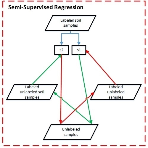
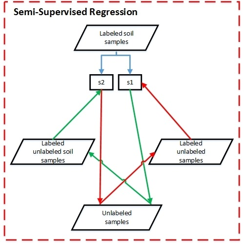
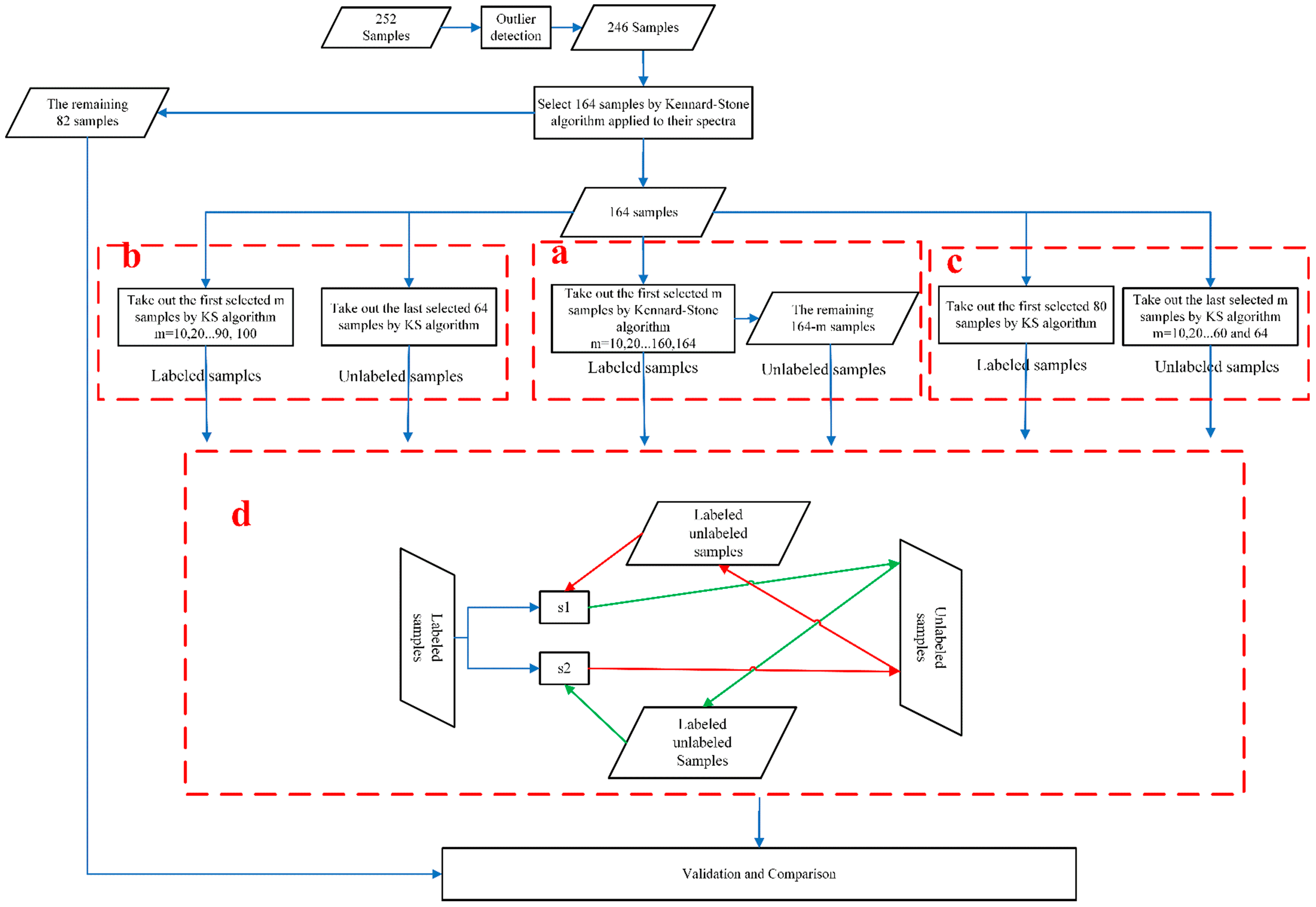
2.2. Semi-Supervised Regression with Co-Training Based on LSSVMR (Co-LSSVMR)

Let L = { ( x 1 , y 1 ) , ( x 2 , y 2 ) , , ( x | L | , y | L | ) } denote the labeled sample set, where x i represents a vector of a soil spectrum, and y i is the associated SOC content. Let U denote the unlabeled sample set, whose soil spectra are available and SOC content values are unknown.
In the SSR with co-training, two regressors are firstly trained with labeled samples, and each regressor is then gradually refined by using the unlabeled samples selected by the other regressor during the co-training progress. In this algorithm, the first key point is building two diverse regressors. In this study, the difference between the two regressors is achieved by using two different kernel functions because the solution of LSSVMR is obtained in a kernel-induced feature space. The second key point is determining the labeling confidence for the unlabeled samples. In the literature [18], the labeling confidence is rated by consulting the influence of each unlabeled sample on the labeled samples, and the sample with the highest labeling confidence is the one that reduces the most of fitting error when used in calibration. In this study, the labeling confidence on each unlabeled sample was measured by the reduction of root mean square error of leave-one-out cross-validation (RMSECV) before and after the sample was added to the training set.
Other two important problems to be addressed in SSR with co-training are the stopping criteria and model selection in learning phases. In theory, a weak learner trained with labeled samples can be raised to an arbitrary precision through the constant use of unlabeled samples [28]. However, experiments have shown that the learning performance could not be improved further after a number of learning iterations [28]. Hence, to avoid overfitting problem, the number of learning rounds is often specified [18]. However, in our initial experiments, a fixed number of learning iterations often failed to select the best model, and thus the learning phase was performed until all potential unlabeled samples were used in this study. RMSECV and root mean square error of calibration (RMSEC) were tested as model selection criterion, and the model with the lowest RMSECV or RMSEC was selected for each regressor.
In Co-LSSVMR, two LSSVMR models ( s 1 and s 2 ) generated from the labeled samples with two kernel functions (RBF and RBF4) were employed to label the unlabeled samples and to determine the labeling confidence. In each iteration, the sample with the highest confidence was used to refine the other learner. The learning process was continued until no unlabeled sample could reduce the RMSECV of the two models. After the learning phase, one model was selected for each regressor based on model selection criterion. The final estimation was obtained by averaging the estimations of these two refined models. The steps of Co-LSSVMR are illustrated in Figure 1 and summarized as follows:
(1)
Copy labeled set L to L 1 and L 2 .
(2)
Train two LSSVMR regressors s 1 and s 2 from L 1 and L 2 with RBF and RBF4 as their kernel functions, respectively.
(3)
Obtain labeling set U 1 and U 2 from the unlabeled set U using s 1 and s 2 , respectively.
(4)
Add the most confidently labeled sample x u of U 2 to L 1 , and remove x u from U 1 and U 2 . x u is the one that results in the largest reduction of RMSECV of s 2 .
(5)
Add the most confidently labeled sample x u of U 1 to L 2 , and remove x u from U 1 and U 2 . x u is the one that results in the largest reduction of RMSECV of s 1 .
(6)
Retrain s 1 and s 2 , and update the labeling values of U 1 and U 2 with s 1 and s 2 , respectively.
(7)
Repeat Steps (4)–(6) until neither L 1 nor L 2 changes.
(8)
Select a refined model for each regressor ( s 1 and s 2 ) according to the model selection criterion.
(9)
For a sample to be estimated, the average of the estimations of the two refined models is considered the final estimation.

3. Materials and Methods

3.1. Study Area and Field Sampling

Honghu City (113°07′–114°05′E, 29°38′–30°12′N) is situated in the north shore of the middle reaches of the Yangtze River and the central south of Hubei Province, China. It has a mean annual temperature of 16.6 °C and a mean annual precipitation ranging from 1000 to 1300 mm. The landform is flat and vast, with an average elevation less than 50 m. The parent material is dominated by quaternary alluvial deposits and lacustrine sediments, and the main soil types are paddy (Anthrosols) and fluvo-aquic soil (Gleysols) [29,30].
A total of 252 soil samples were collected in four field campaigns (108 on 20–21 December 2011, 60 on 10–11 July 2012, 40 on 17–19 November 2012 and 44 on 14–15 April 2013), 180 of which were fluvo-aquic soil and the others were paddy soil. At each sampling point, about 1.0 kg of surface soils (0–10 cm) was collected after wiping off plant material, plant residues, roots and stones. Each soil sample was kept in a sealed package for spectral measurement and SOC content determination in the laboratory.

3.2. Laboratory Analyses and Measurements

After being air-dried at an indoor temperature for three days and removing stones and plant residues, all soil samples were ground with an agate mortar and passed through a 20-mesh sieve (<2 mm). Each sample was placed in a 10 cm-diameter petri dish. The geometric conditions of the measurement were detailed by Shi [6]. The reflectance spectra were measured in a laboratory through an ASD FieldSpec 3 portable spectroradiometer (Analytical Spectral Devices, Inc., Boulder, CO, USA) with a wavelength range of 350–2500 nm. Its sampling intervals are 1.4 in the 350–1000 nm range and 2 in the 1000–2500 nm range, and its spectral resolutions are 3 nm in the 350–1000 nm range and 10 nm in the 1000–2500 nm range. The measured values are interpolated, and the spectroradiometer finally provides a spectrum of 2151 bands with a uniform spectral interval of 1 nm. Correction with a standardized white Spectralon panel (Labsphere, Inc., North Sutton, NH, USA) with near 100% reflectance was performed prior to each scan. An average value of 10 spectral measurements for each sample was calculated as the final reflectance spectrum. After spectral measurements were made, the SOC contents of all soil samples were determined using the Walkley and Black method [31] in the laboratory, which is based on wet oxidation in potassium dichromate.

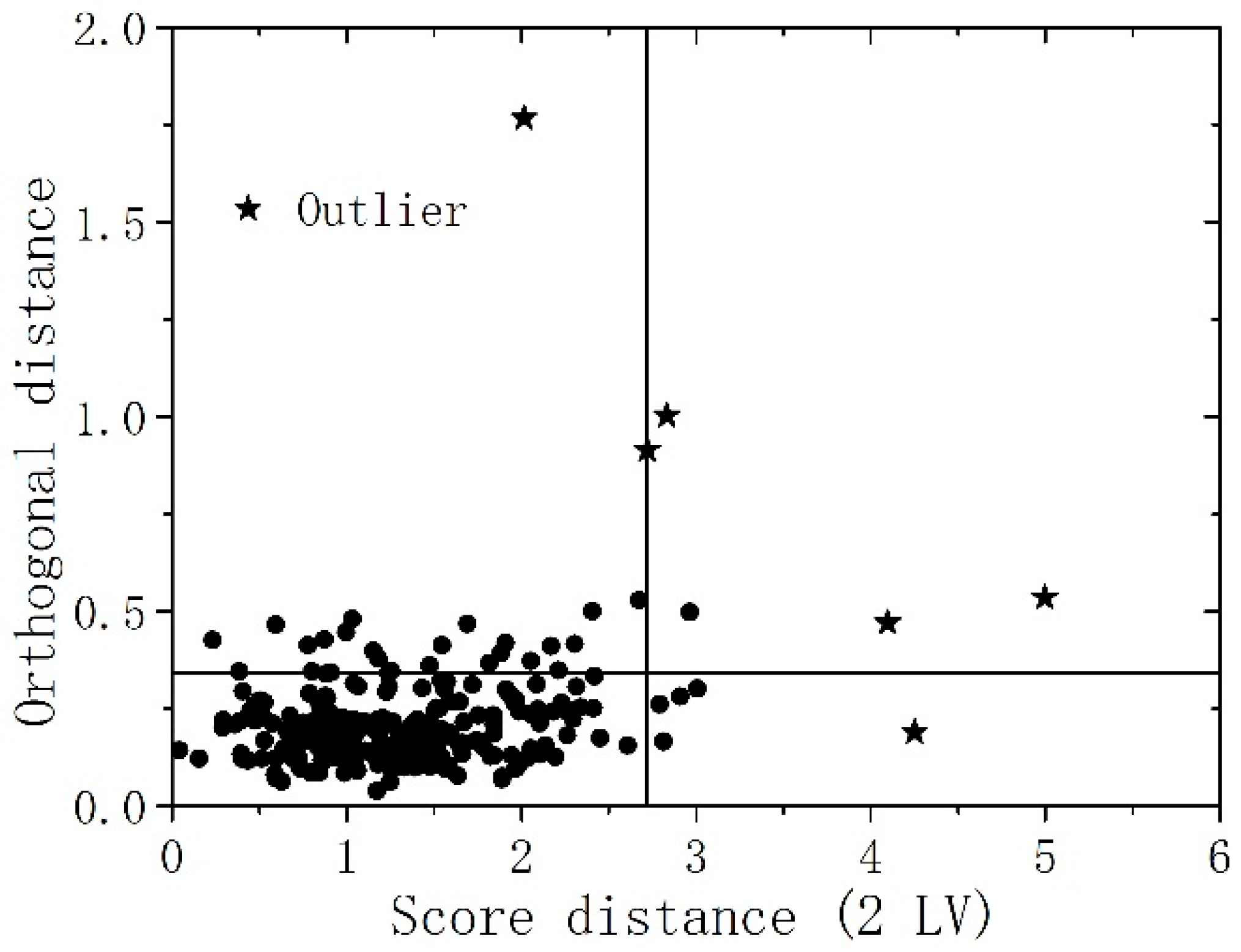
3.3. Spectral Preprocessing and Outlier Detection

Considering the high noise effects at spectral edges, the reflectance spectra were reduced to 400–2450 nm and then smoothed with the Savitzky–Golay smoothing method [32] with a second order polynomial fit and a window size of 9 data points. The outliers were detected using robust principal component analysis (ROBPCA) method, and samples with a large score distance and a large orthogonal distance within the principal component analysis (PCA) subspace were identified as outliers. The ROBPCA was implemented through a Matlab toolbox provided by Verboven and Hubert [33]. Six outliers (Figure 2) were detected and eliminated.
To reduce data dimensionality and to match the finer spectral resolution of the spectroradiometer, the reflectance spectra were resampled using 3-nm spacing intervals, providing 681 variables. The SOC contents of the remaining samples were statistically described. The soil samples were divided equally in number into four groups based on SOC content values from low to high, and the average spectrum of each group was calculated, visualized and analyzed.

3.4. Model Calibration

Models were calibrated using the settings in Figure 1a–c, respectively, to investigate the sensitivity of SSR to the percentage of labeled samples, and the number of labeled and unlabeled samples. A total of 164 out of the 246 samples were selected as candidate calibration dataset through Kennard-Stone (KS) algorithm [34]. The selected samples were recorded in the order produced by the KS algorithm. The remaining 82 samples were used as the validation dataset. For investigating the sensitivity of SSR to the percentage of labeled samples, the first m samples (m = 10, 20, …, 160, and 164) out of the 164 samples were considered as labeled samples, and the remaining 164–m samples were used as unlabeled samples in Co-LSSVMR. Considering the popularity of the partial least square regression (PLSR) in SOC content estimations [35], PLSR models were also calibrated only with the first m labeled samples and compared with LSSVMR and Co-LSVMR models.
In the above experiments, the gains in estimation accuracy were mitigated when 100 out of the 164 samples were used as labeled samples. For assessing the sensitivity of Co-LSSVMR to the number of labeled samples, the unlabeled samples were kept invariant. The last 64 samples out of the 164 samples were used as unlabeled samples, and the first m samples (m = 10, 20, …, 100) were used as labeled samples for Co-LSSVMR. The model performance was studied by increasing the labeled samples size gradually.
For investigating the sensitivity of Co-LSSVMR to the number of unlabeled samples, the labeled samples used for calibration were kept invariant. The first 80 out of the 164 samples were used as labeled samples, and the following 10, 20, …, 60, and 64 samples were considered as unlabeled samples. The model performance was studied by increasing the dataset size of unlabeled samples gradually.

3.5. Model Evaluation and Comparison

For comparing the performance of LSSVMR and Co-LSSVMR, the average of SOC estimations obtained by the two initial LSSVMR models calibrated only with labeled samples was considered as the estimation of the LSSVMR. The estimation performance was evaluated using the validation dataset, and the accuracy was assessed by the RMSE of validation (RMSEV), coefficient of determination (R2v) and ratio of inter-quartile range to RMSEV (RPIQ) [36,37]. Bellon-Maurel et al. [37] suggested that RPIQ, based on quartiles, might be a better indicator for performance estimation than residual prediction deviation (RPD). Moreover, the gains in estimation accuracy obtained by Co-LSSVMR with respect to LSSVMR were obtained by subtracting the RMSEV of Co-LSSVMR from RMSEV of LSSVMR and then dividing the result by the RMSEV of LSSVMR.
All programs, including spectra preprocessing, parameter optimization and modeling, were implemented in MATLAB 7.11.0 (www.mathworks.com), and the parallel computing toolbox was used to improve computing efficiency. The LS-SVMlab toolbox [27] was used to implement the LSSVMR.

4. Results

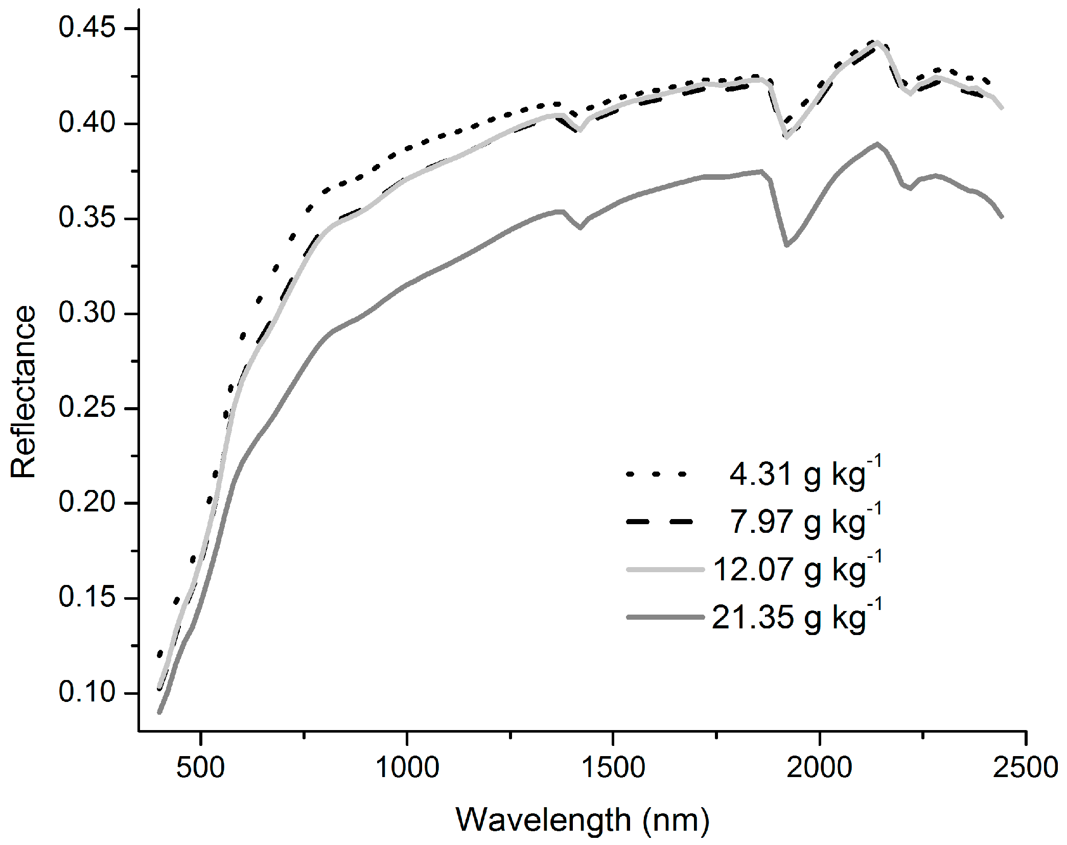
4.1. Descriptive Statistics and Reflectance Spectra of Soil Samples

The statistical descriptions of SOC contents for the whole, candidate calibration and validation datasets are shown in Table 1. The SOC contents for the whole dataset varied from 0.76 to 45.73 g·kg−1, with an average value of 11.51 g·kg−1 and a median value of 10.04 g·kg−1. The distributions of the whole, calibration and validation datasets showed a positively skewed distribution with a skewness of 1.01, 1.26 and 0.65 and a kurtosis of −0.83, 2.74 and 1.28, respectively.
The average reflectance curves show the typical patterns of soil spectra in the VIS-NIR regions with three prominent absorption features around 1400, 1900 and 2200 nm (Figure 3). The absorption region near 1400 nm is the first overtone of OH stretches, and the second region near 1900 nm is due to the combination of OH stretches and H–O–H bend [38]. The absorption near 2200 nm results from OH stretches and Al/Fe–OH bend [25]. The average reflectance with 4.31 g·kg−1 SOC is the highest, and that with 21.35 g·kg−1 SOC is the lowest. However, the spectra curves of the two other groups are very close to each other, possibly indicating the non-linear relationship between spectra and SOC contents, as SOC and other soil elements combine to produce a soil spectrum.

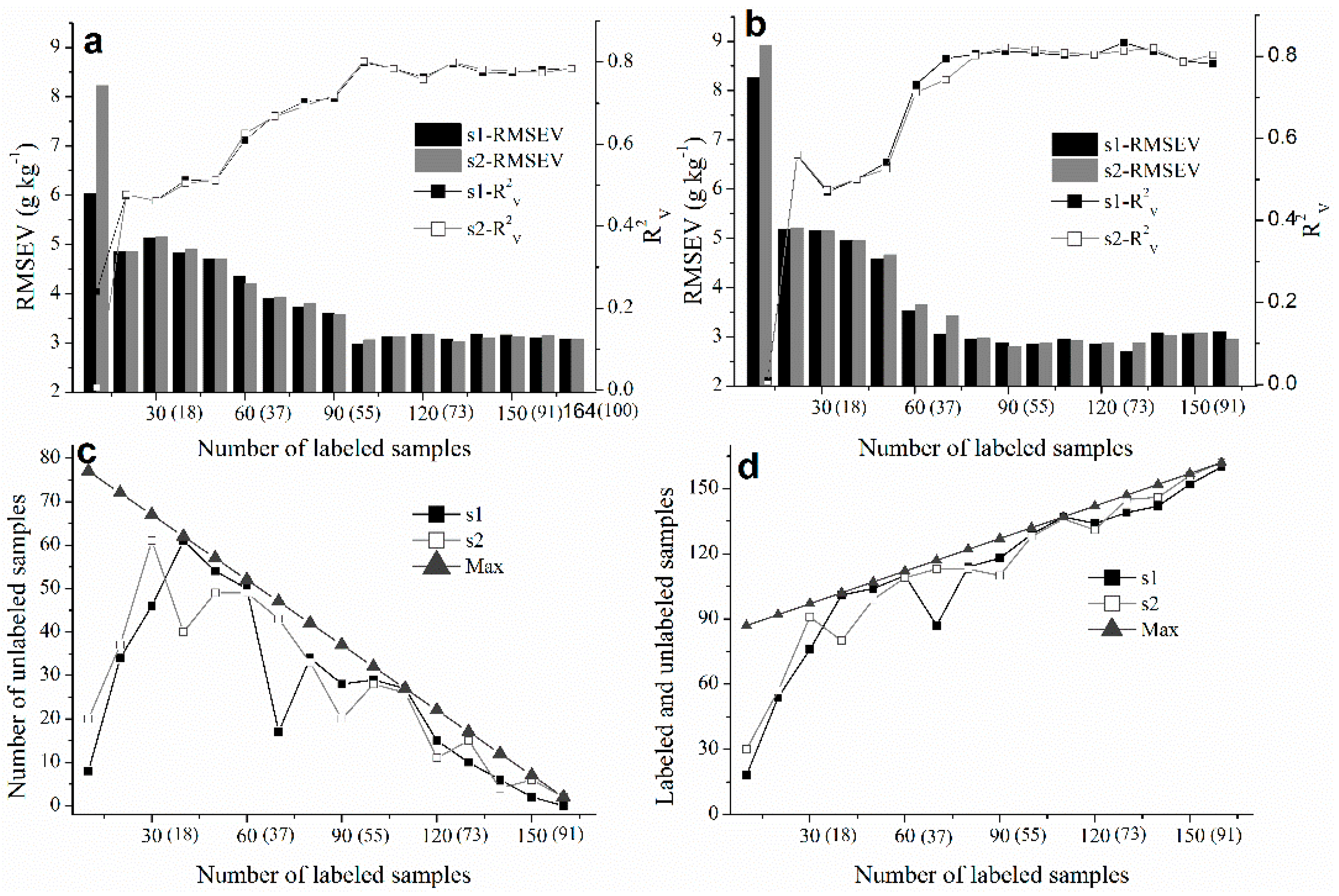
4.2. Sensitivity to the Percentage of Labeled Samples

To illustrate the models’ behavior in the co-training process, the RMSECV, RMSEC and RMSEV of the two regressors with regard to the number of unlabeled samples exploited are plotted for the scenarios of 10, 70 and 150 labeled samples used in the calibration (Figure 4). For these three cases, the RMSECV of the two regressors exhibited a decreasing trend as more unlabeled samples were incorporated in the calibration, whereas the RMSEC and RMSEV displayed different patterns. When only 10 labeled samples were used, a clear overfitting phenomenon was observed with RMSEC close to 0, whereas the validation performance of the two regressors deteriorated gradually. The calibration and validation accuracies of the two regressors obviously increased when 70 labeled samples were used. For 150 labeled samples, a slight improvement was observed for RMSEC and RMSEV.
In addition to the 10 labeled samples, the overfitting phenomena were observed when no more than 40 labeled samples were used in the calibration, which indicated that 40 samples were not sufficient to capture the SOC variations for this study area. Therefore, the cases with less than 40 labeled samples were not considered in determining the model selection criterion. The RMSE versus RMSEC and RMSE versus RMSECV are plotted (Figure 5 and Figure 6) to examine the relationships of model performance with calibration accuracy and cross-validation accuracy. In most cases, RMSEV values had a similar increasing or decreasing trend with RMSEC (Figure 5); whereas RMSEV exhibited weak correlations with RMSECV (Figure 6) because the decrease in RMSECV did not surely result in a decrease in RMSEV. Thus, the RMSEC was selected as the model selection criterion, and the refined model for each regressor was selected according to the lowest RMSEC. Moreover, the cases with fewer than 40 labeled samples in calibration also adopted this model selection criterion.
The percentage of labeled samples used in calibration had an obvious effect on the estimation accuracies of the models trained only with labeled samples as well as the refined models of Co-LSSVMR. In general, more labeled samples were more likely to result in better estimation performance (Figure 7a,b). When only 10 labeled samples were used, both models produced poor estimations with high RMSEV and low R2V. The performances of the two LSSVMR models were improved gradually as the number of the labeled samples increased to 100, in which the performance leveled (Figure 7a). No notable improvement was observed for the two refined models in Co-LSSVMR as the number of the labeled samples increased from 20 to 50; however, the estimation accuracies improved remarkably as the number of labeled samples increased from 50 to 60. Thereafter, the performances of both models were improved until they leveled at 80 labeled samples.
The number of unlabeled samples exploited and the total number of labeled and unlabeled samples used by each refined model in Co-LSSVMR are summarized in Figure 7c,d. The number of unlabeled samples used by each refined model increased quickly as the number of labeled samples increased from 10 to 30. The number displayed a decreasing trend when more than 50 labeled samples were used, which was approximately consistent with the maximum number of unlabeled samples available for each regressor. For the total number of labeled and unlabeled samples used by each refined model, the increasing trend was approximately consistent with the maximum number available for each regressor when more than 30 labeled samples were used in the calibration.
Figure 8 illustrates and compares the final estimation performances of LSSVMR and Co-LSSVMR. The RMSEV obtained by LSSVMR reduced gradually from 5.16 g·kg−1 at 30 labeled samples (RPIQ = 1.97, R2V = 0.46) to 3.12 g·kg−1 at 100 labeled samples (RPIQ = 3.31, R2V = 0.79), and then it turned relatively stable. The RMSEV obtained by Co-LSSVMR decreased sharply from 4.62 g·kg−1 at 50 labeled samples (RPIQ = 2.19, R2V = 0.53) to 3.58 g·kg−1 at 60 labeled samples (RPIQ = 2.84, R2V = 0.73), and further decreased gradually to 2.95 g·kg−1 at 80 labeled samples (RPIQ = 3.44, R2V = 0.81), where it began to level off. The RMSEV obtained by PLSR decreased gradually from 5.90 g·kg−1 at 10 samples to 3.24 g·kg−1 at 110 samples, and then it began to be stable. LSSVMR obtained its best estimations when 130 labeled samples were used (RMSEV = 3.02 g·kg−1, RPIQ = 3.35, R2V = 0.80), and Co-LSSVMR had best estimation accuracy at 110 labeled samples (RMSEV = 2.77 g·kg−1, RPIQ = 3.66, R2V = 0.83). The estimations produced by Co-LSSVMR were better than the best estimation obtained by LSSVMR when over 80 out of 164 samples were labeled samples.
The gains in estimation accuracy achieved by Co-LSSVMR with respect to LSSVMR varied with the percentage of labeled samples used in calibration (Figure 8c). When less than 40 out of the 164 samples were used as labeled samples, Co-LSSVMR had similar or poorer performance when compared with LSSVMR, whereas Co-LSSVMR had an advantage over LSSVMR with over 15% gains in accuracy when 60 to 90 labeled samples were used. Furthermore, the gains in accuracy reached a maximum of 22.52% at 80 labeled samples. The gains in accuracy obtained by Co-LSSVMR were moderate (6.64%, 11.50%, 10.04% and 8.16%) for 100 to 130 labeled samples. When more than 140 samples were labeled, Co-LSSVMR produced slightly better estimations than LSSVMR with gains in accuracy smaller than 5%.
The calibration and validation results obtained by LSSVMR and Co-LSSVMR when 80 labeled samples were used for calibration are illustrated and compared in Figure 9. The LSSVMR obtained acceptable fitting accuracy with samples scattering around the 1:1 line (Figure 9a,b), however, it tended to overestimated low SOC values and underestimated high SOC values with a slope of 0.60 and an intercept of 4.05 g·kg−1 (Figure 9c). By exploiting the unlabeled samples, Co-LSSVMR obtained better fitting accuracy (Figure 9e,f) and validation performance with a slope of 0.76 and an intercept of 2.45 g·kg−1 (Figure 9g).

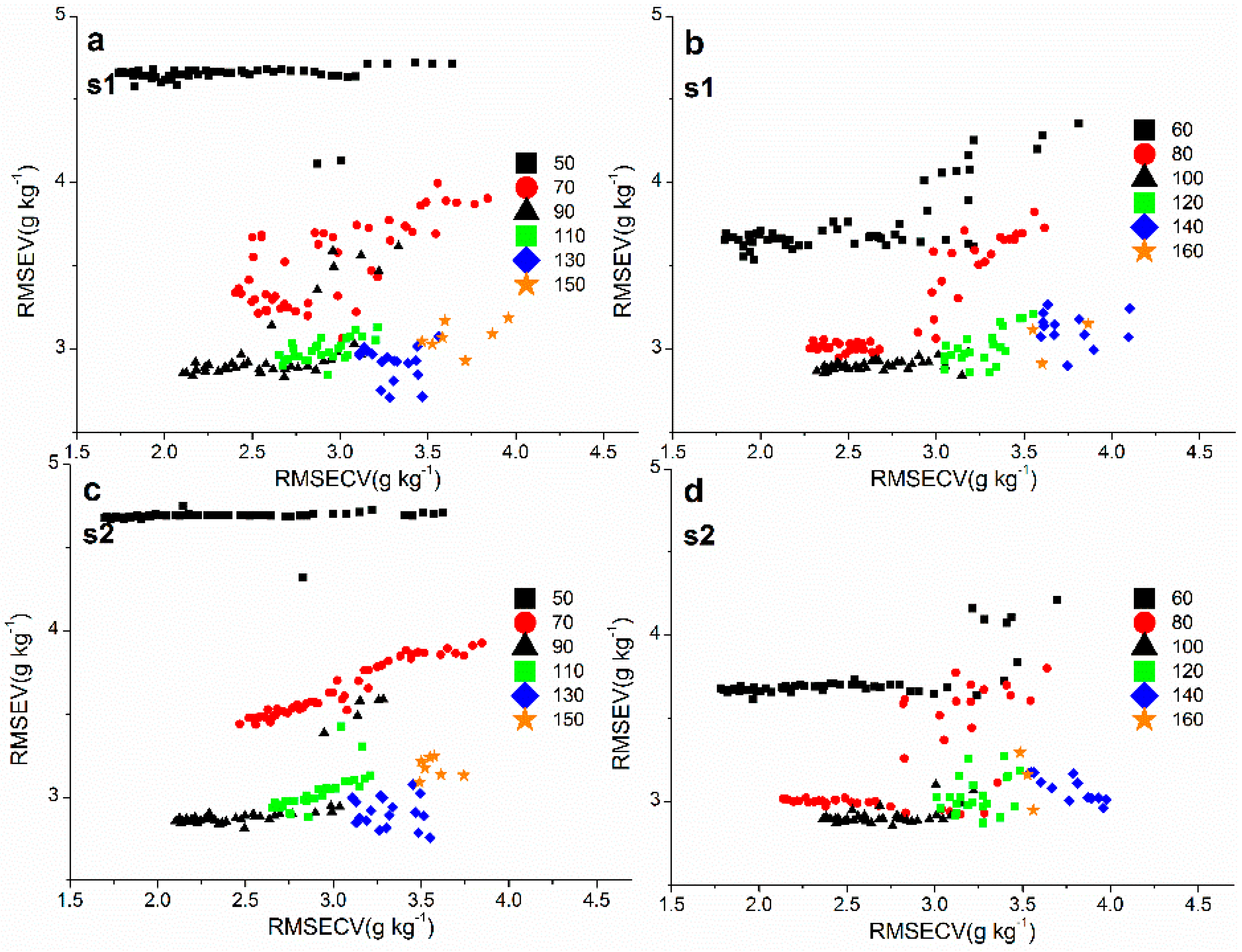
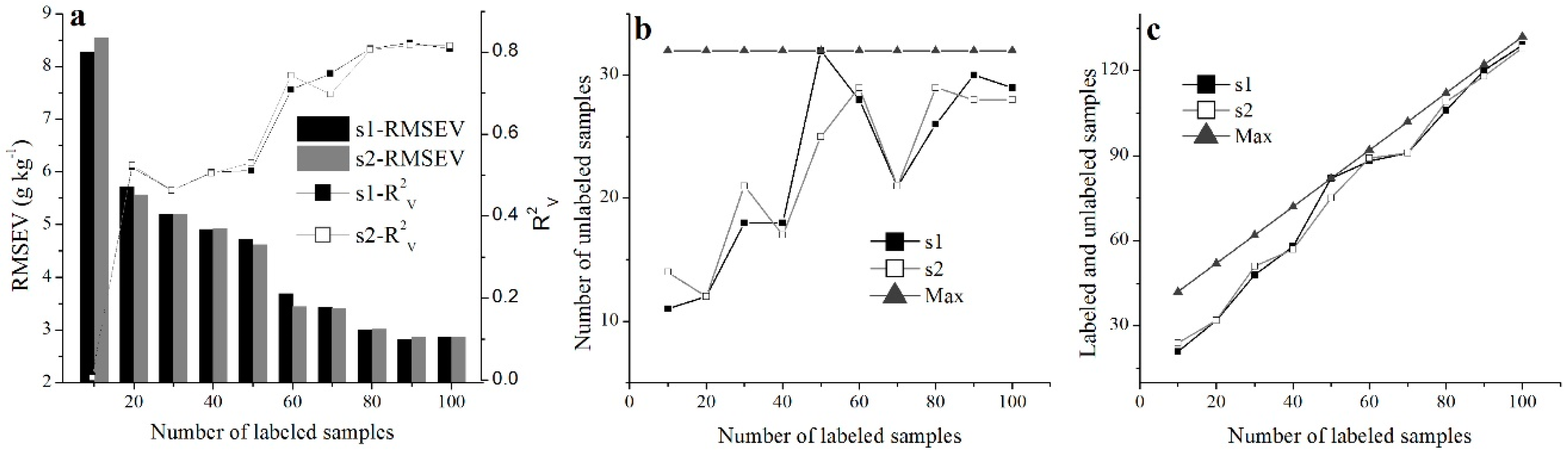
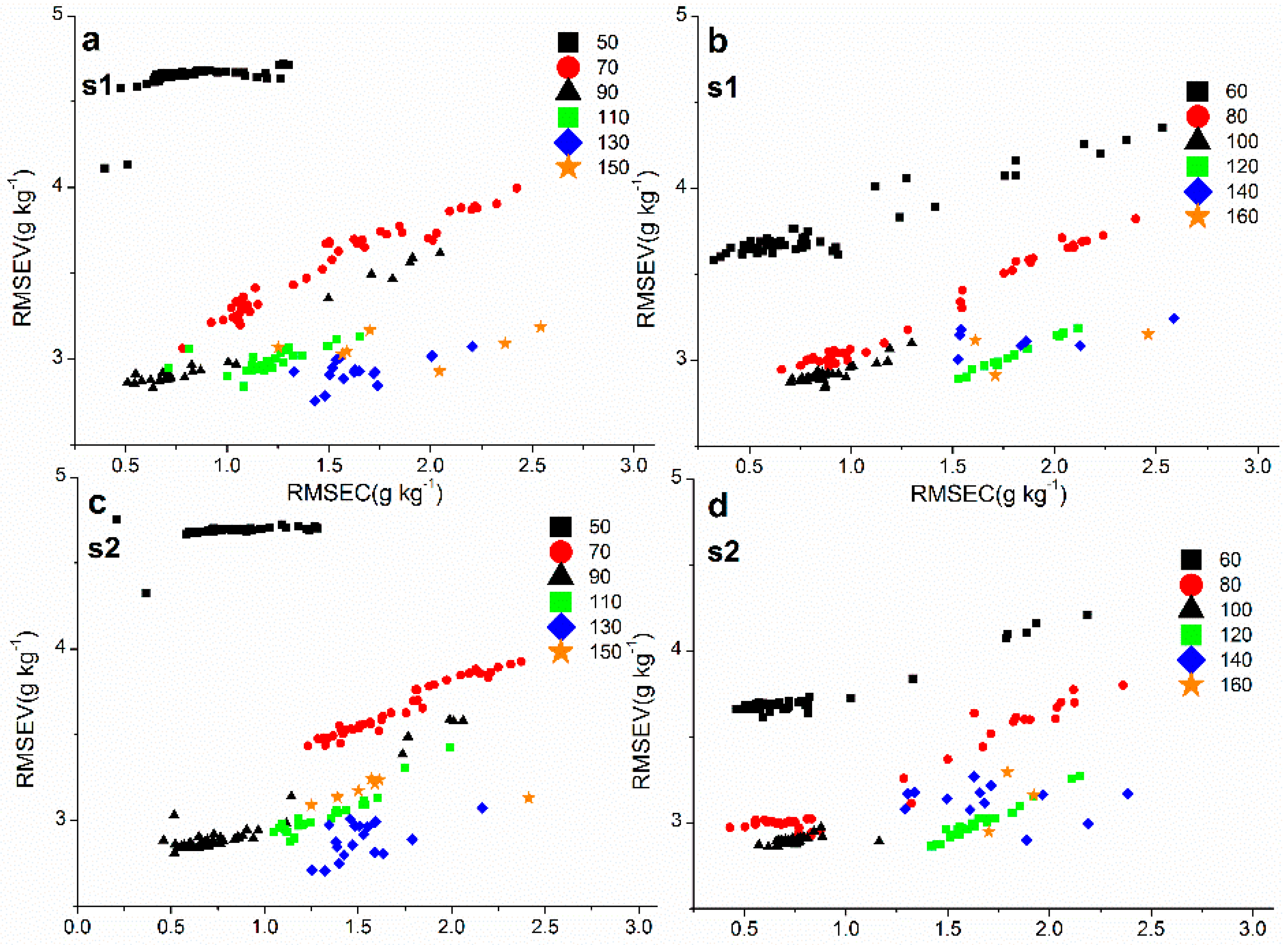
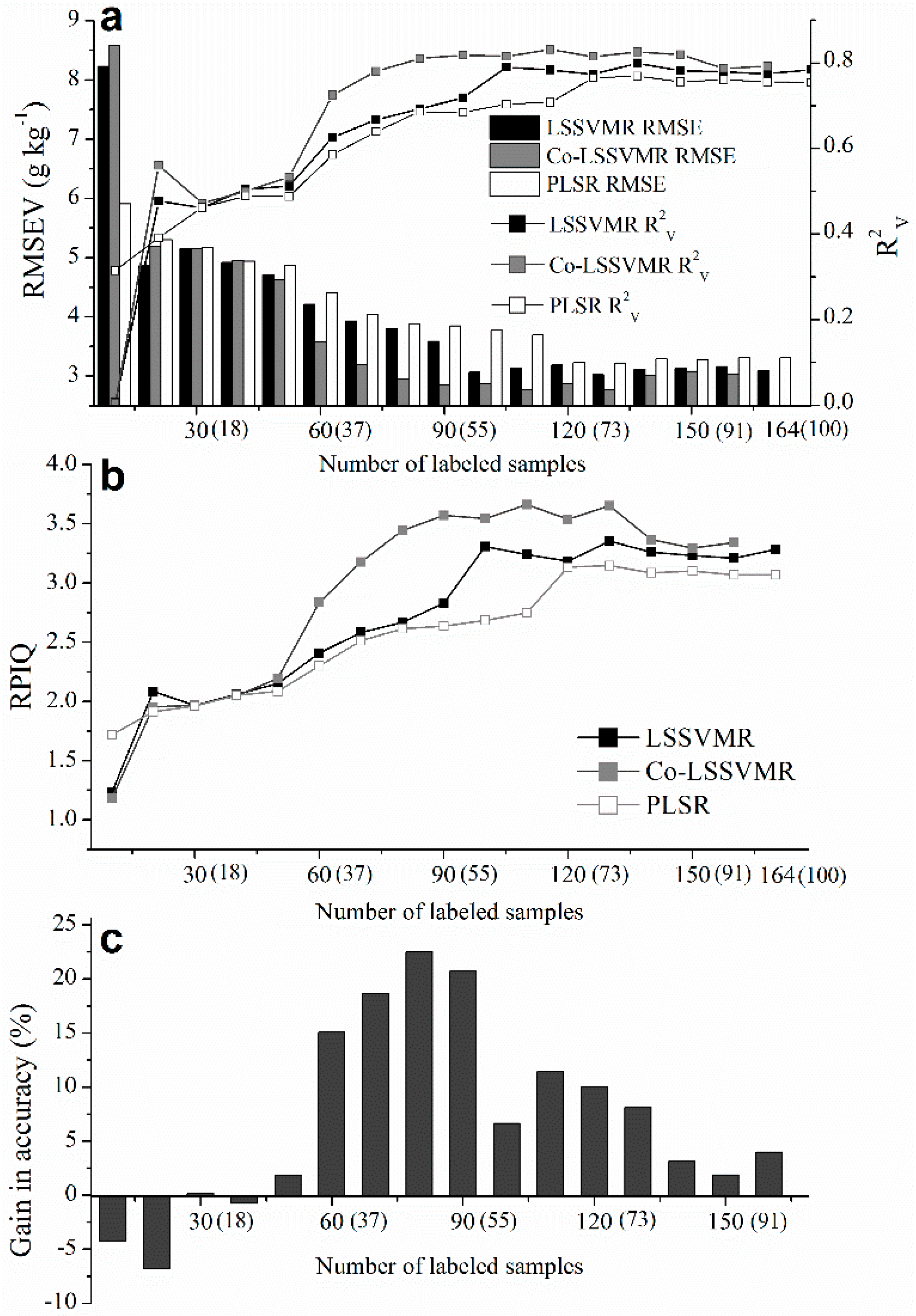
4.3. Sensitivity to the Number of Labeled Samples

Figure 10 and Figure 11 show the results obtained by Co-LSSVMR with respect to its sensitivity to the number of labeled samples. The performances of the two refined models in Co-LSSVMR and their average estimations exhibited similar patterns, improving gradually as the number of the labeled samples increased from 20 to 80. The number of the unlabeled samples included in each refined model showed an upward trend as the number of labeled samples increased from 10 to 40 (Figure 10b), while the total number of labeled and unlabeled samples in each refined model displayed an increasing trend as the number of labeled samples increased constantly (Figure 10c).
The effectiveness of Co-LSSVMR was sensitive to the number of labeled samples (Figure 11). The Co-LSSVMR produced less accurate estimations than LSSVMR when less than 40 labeled samples were used in the calibration. In addition, the gains in accuracy obtained by Co-LSSVMR were negligible even though 57 unlabeled samples were exploited when the size of the labeled samples was 50. However, Co-LSSVMR produced notable gains in accuracy ranging from 13% to 21% when 60 to 90 labeled samples were used. The gains in accuracy were reduced to 6.64% when the number of labeled samples was 100.

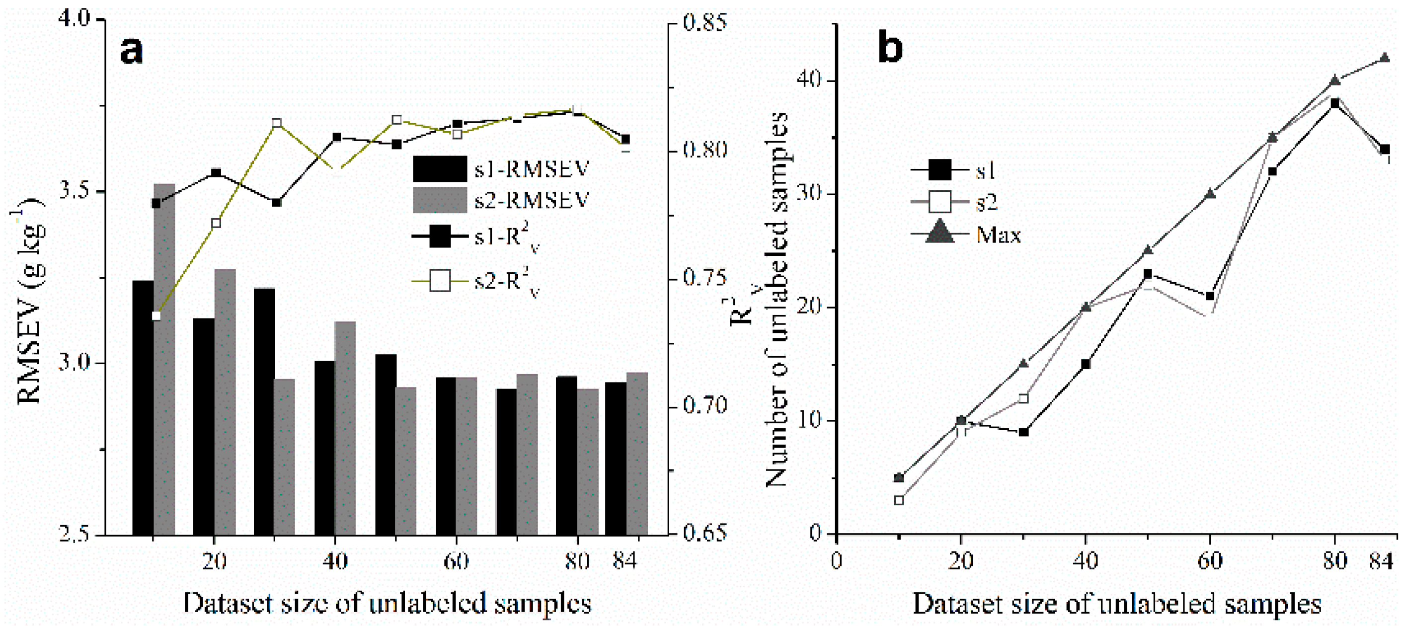
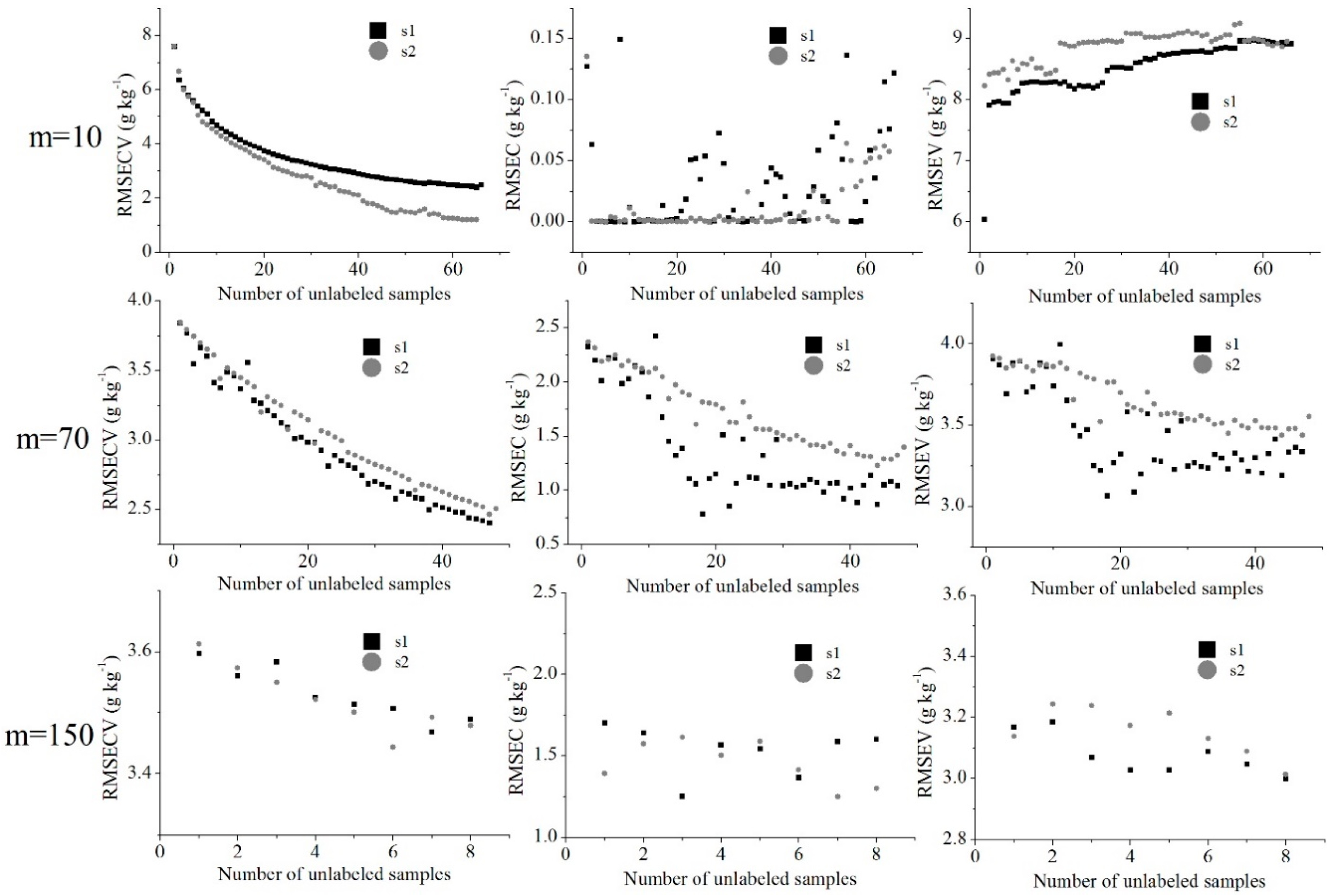
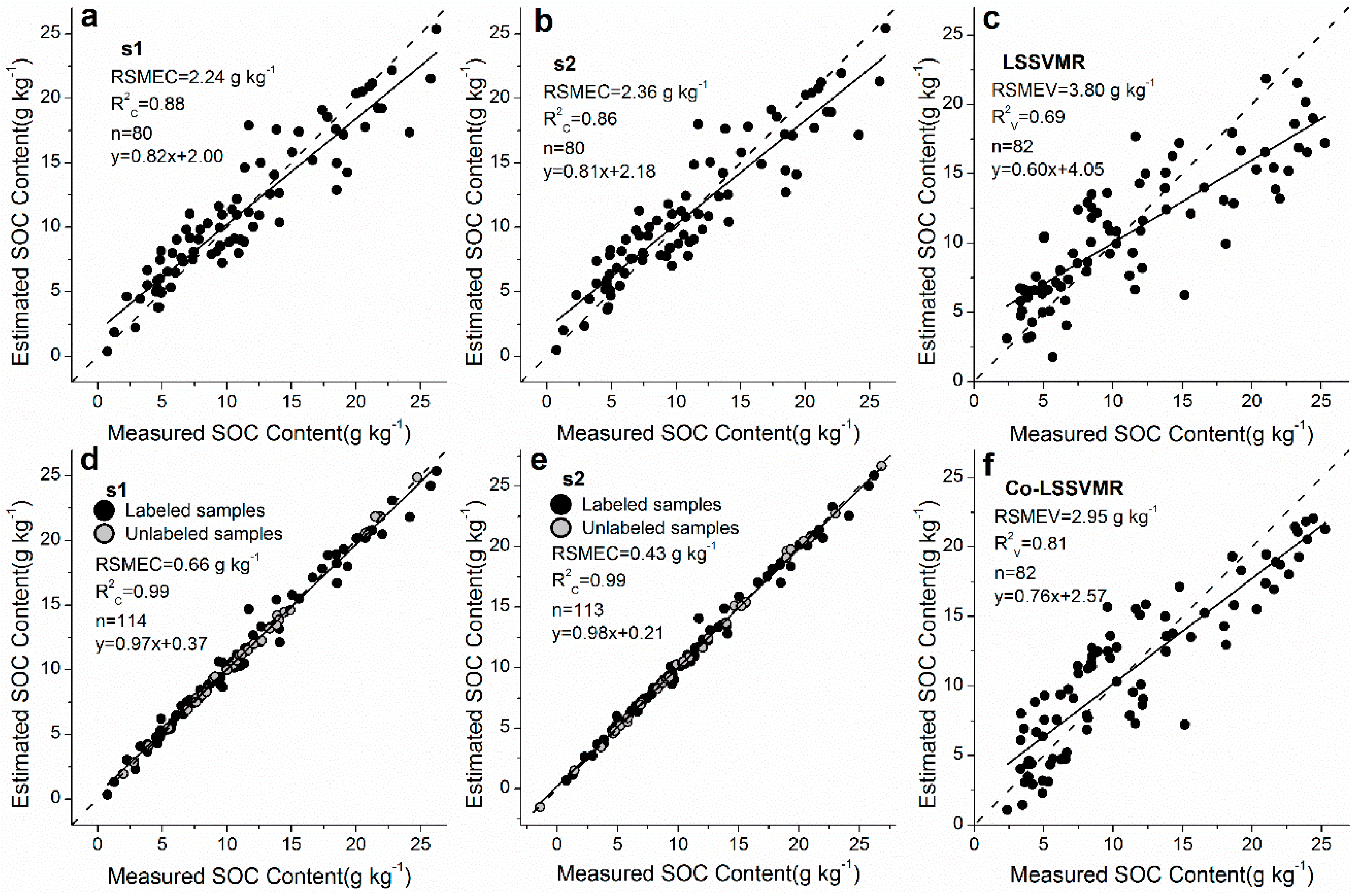
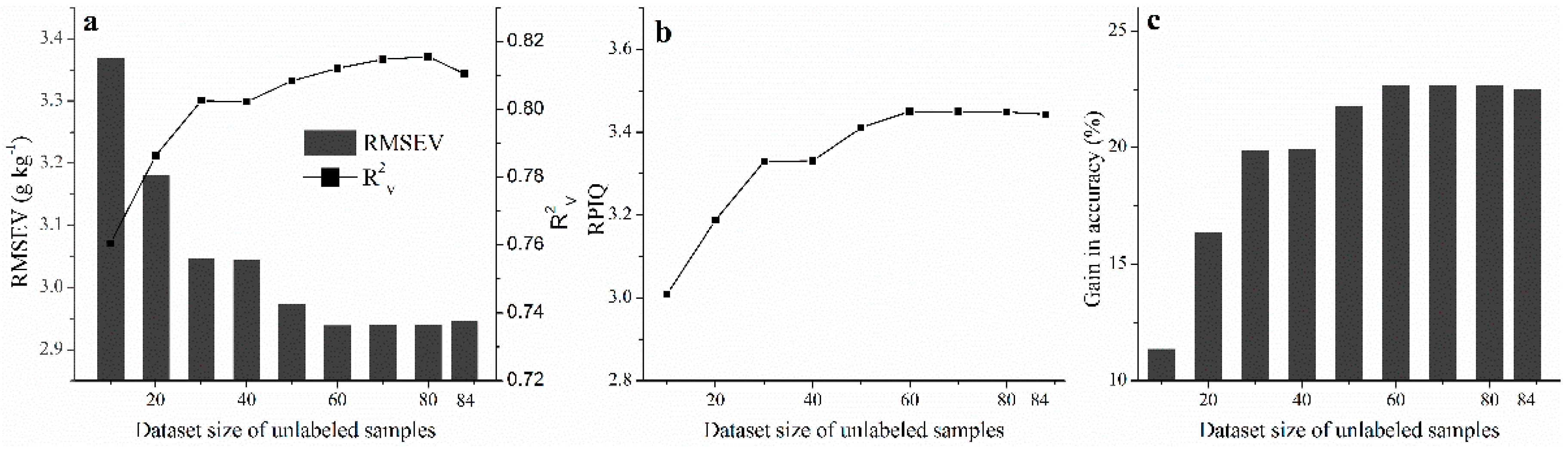
4.4. Sensitivity to the Number of Unlabeled Samples

The results obtained by Co-LSSVMR with 80 labeled samples are summarized in Figure 12 and Figure 13, which show the sensitivity of Co-LSSVMR to the pool size of unlabeled samples. The RMSEV obtained by each refined model and the difference of the RMSEV of the two refined models exhibited decreasing trends as the pool size of unlabeled samples increased from 10 to 60, whereas the number of unlabeled samples exploited by each model displayed an increasing trend. The differences of the RMSEVs of the two refined models were larger than 0.1 g·kg−1 when less than 50 unlabeled samples were available. Thereafter, the estimation performances of the two regressors tended to level off and be comparable as more unlabeled samples were available and incorporated.
The estimation accuracies of Co-LSSVMR, RMSEV decreased gradually as the dataset size of unlabeled samples increased from 10 to 60, whereas R2V, RPIQ and the gains in estimation accuracy showed increasing trends (Figure 13). Co-LSSVMR obtained good estimations with 11.36% gains in accuracy over LSSVMR when the pool size of unlabeled samples was 10. The gains in accuracy were greater than 20% when the pool size of unlabeled samples was larger than 50. The estimation performance remained stable when more than 60 unlabeled samples were available.

5. Discussion

This study demonstrated the effectiveness of SSR in estimating SOC contents from VIS-NIR spectroscopy when the number of labeled samples was limited but not excessively small. SSR is based on the assumptions that the data lie on a low-dimensional manifold embedded in a higher-dimensional space and similar inputs should have similar outputs [13]. These assumptions are valid for the scenario of estimating SOC contents with VIS-NIR spectroscopy, since they are similar to spectral matching in soil spectroscopy, which has been applied successfully to SOC contents as well as other soil characteristics estimations [39,40,41,42]. SSR obtained better SOC estimations because the unlabeled data provided helpful information on the ground-truth data distribution [43]. This statement was confirmed by our results in Figure 9, which shows that the extra unlabeled samples included in the refined models make each model more consistent with the labeled samples and accordingly produce better performance for the validation dataset.
This study found that SSR produced few model improvements or even reduced model performance when less than 50 labeled samples were used. The labeling confidence for unlabeled samples estimated by the amount of reduction of RMSECV on the labeled samples was not reliable, which was also observed by other studies [19,43,44], and such result could be explained by that a small sample dataset was not sufficient to capture information sufficient to describe the soil variations. Thus, overfitting phenomena were more likely to occur when the number of labeled samples used in calibration was small, which indicated that the model had poor generalization performance although it fitted perfectly well for the training dataset. Given the poor performance for the validation dataset, the labeling quality for the unlabeled samples should not be high, and more noises than useful information might be introduced by the addition of unlabeled samples.
We also found that SSR appeared to be more useful when the percentage of labeled samples was neither excessively large nor excessively small. As mentioned above, the performance degradation occurred at small labeled-sample size could be attributed to unreliable labeling confidence evaluation and low labeling quality. However, the labeling confidence became more reliable, and the labeling quality became high as more labeled samples were used. Thus, SSR could capture more useful information from unlabeled samples to improve the estimation accuracy. However, the usefulness of SSR seemed to be limited when the percentage of labeled samples was large enough. This finding might be explained by the following: (i) the high estimation accuracy obtained only with the labeled samples left little room for improvement [44,45]; and (ii) only a small number of unlabeled samples available for exploitation might reduce the probability of selecting highly informative unlabeled samples. Moreover, the results obtained under the fixed number of unlabeled samples exhibited a similar trend to the number of labeled samples.
Co-LSSVMR needed less labeled samples than LSSVMR to achieve good estimations, which could be explained by that the estimation performance of Co-LSSVMR improved more quickly through the use of unlabeled samples as the labeled-sample size increased. However, this study also indicated that estimating SOC contents accurately with very few labeled soil samples through SSR might be impractical. In some applications, SSL appeared to require significantly fewer labeled samples than its corresponding supervised technique in obtaining high accuracy [45], whereas the usefulness and performance of SSL was also found to be dependent on the complexity of the problems to be solved and the labeled sample size [19,44,45]. Viscarra Rossel [4] pointed out that sufficient samples, which can adequately describe the soil variation of the study area, were required for the high estimation accuracy of soil properties. The complex relationship between SOC content and soil reflectance might explain the failure to achieve accurate estimations with very few labeled samples, because soil spectrum is determined by the combinations of absorption features from different mineral components and organic matter [46,47].
We found that the effectiveness of SSR was also influenced by the dataset size of unlabeled samples. To some extent, more unlabeled samples available for exploitation were more likely to cause more gains in accuracy. Notable performance differences between the two regressors in Co-LSSVMR were observed when a limited number of unlabeled samples were available. This finding also indicated the improvement potential left for refinement, which was confirmed by the further improvements obtained with larger dataset size of unlabeled samples.
In this study, no extra stopping criteria were adopted to terminate the learning phases because of the limited number of unlabeled samples. However, testing all unlabeled samples exhaustively from a large dataset is inefficient. It is especially true for hyperspectral imaging applications, in which a large population of soil spectra can be collected [48,49,50]. In such a scenario, testing all available unlabeled samples is impractical. In addressing this problem, a representative subset of unlabeled samples must be extracted in advance [18]. Bazi et al. [19] compared three unlabeled sample selection strategies based on random sampling, variance and differential entropy and found that differential entropy outperformed the other two strategies. This study could be a good reference for future applications of SSR in estimating SOC contents with hyperspectral images.
Several modeling strategies and techniques have been explored in literatures to improve the estimations of SOC contents from hyperspectral spectroscopy. For example, Local regression is a promising modeling strategy especially for diverse datasets with large soil variations [40,42,51]. Testing the applicability of the SSR to large diverse and heterogeneous soil spectral dataset [52,53] would be a meaningful task in the future. Moreover, investigating the compatibility of SSR with these modeling strategies and techniques might be meaningful for further studies.

6. Conclusions

This study investigated the effectiveness of SSR in estimating SOC contents from laboratory-based VIS-NIR spectroscopy with a limited number of samples with reference values. The principal conclusions obtained can be summarized as follows:
(1)
Co-LSSVMR can generally produce better estimations than LSSVMR when the number of labeled samples is not excessively small (>50), and the gains in accuracy of Co-LSSVMR with respect to LSSVMR can be up to over 20%.
(2)
SSR requires less labeled samples to produce estimations of a certain accuracy.
(3)
The usefulness of SSR is sensitive to the number of labeled and unlabeled samples, and SSR is more likely to produce more gains in estimation accuracy when the number of labeled samples is neither excessively small nor excessively large, and when the unlabeled samples are sufficient.

Acknowledgments

This study was supported by the Scientific Research Foundation for Newly High-End Talents of Shenzhen University and Basic Research Program of Shenzhen Science and Technology Innovation Committee (No. JCYJ20151117105543692) and Science and Technology Bureau of Suzhou (No. SYN201309). We greatly appreciated the editor and four anonymous reviewers for their constructive suggestions and insightful comments, which helped us greatly to improve this manuscript.

Author Contributions

All authors conceived and designed the study. Huizeng Liu, Tiezhu Shi and Guofeng Wu made substantial contributions to experiments design. Huizeng Liu implemented the experiments. Yiyun Chen made substantial contributions to the field campaigns, spectral measurements and soil properties determinations. All authors discussed the basic structure of the manuscript, and Huizeng Liu finished the first draft. Tiezhu Shi, Guofeng Wu, Junjie Wang and Teng Fei reviewed and edited the draft. All authors read and approved the submitted manuscript, agreed to be listed and accepted the version for publication.

Conflicts of Interest

The authors declare no conflict of interest.

Appendix A. Least Square Support Vector Machine Regression (LSSVMR)

In LSSVM, a linear estimation is done in a kernel-induced feature space ( y   =   ω T ϕ ( x ) +   b ), where ϕ ( x ) denotes the feature map. In LSSVMR, the error ξ i quadratic norm is taken as the LSSVMR’s loss function by Suykens [22]. The optimization problem is described as follows:
m i n   J ( ω ,   ξ ) =   1 2 ω T ω +   1 2 γ i = 1 | L | ξ i 2
Subject to the equality restriction
y i =   ω T ϕ ( x i ) + b + ξ i   ,   i = 1 ,   2 ,   ,   | L |
The first part of this cost function is a weight decay, which is used to regularize weight sizes and penalize large weights. Large weights will deteriorate the generalization ability of the LSSVMR because they can cause excessive variance, so the weights converge to smaller values. The second part of Equation (A1) is the regression error for all training data. The parameter γ is the punishment factor, which determines the tradeoff between the complexity of the LSSVMR model and its accuracy in capturing the training data. The restriction supplied by Equation (A2) gives the definition of the regression error. For the optimization problem, the Lagrange function is introduced as follows:
L ( ω ,   b . ξ , α ) =   1 2 ω T ω +   1 2 γ i = 1 | L | ξ i 2 +   i = 1 | L | α i [ ω T ϕ ( x i ) + b + ξ i y i ]
In Equation (A3), α i (i = 1, 2, …, | L | ) is the introduced Lagrange multiplier [54]. To obtain the optimum, partial first derivatives of L with respect to each variable are computed and set to zero. According to the Karush–Khun–Tucker (KKT) conditions, ω and ξ can be eliminated through the two following equation:
ω i = 1 | L | α i ϕ ( x i ) = 0
γ i = 1 | L | ξ i γ = 0
An important result of this approach is that the weights (ω) can be written as linear combinations of the Lagrange multipliers with the corresponding data training ( x i ). The Lagrange multiplier α vector and b follows from solving a set of linear equations:
[ K + I γ   1 | L | T 1 | L | 0 ] [ α b ] =   [ y 0 ]
where K denotes the kernel matrix with ij t h element being ϕ ( x i ) T ϕ ( x j ) and I denotes the identity matrix | L | × | L | , 1 | L | = [ 1 ,   1 ,   1 ,   ·   ·   · ,   1   ] T . K ( x i ,   x ) =   ϕ ( x i ) T ϕ ( x ) is the so-called kernel function. Thus, the original regression function ( y =   ω T ϕ ( x ) +   b ) can be replaced by the following one:
y   =   i = 1 | L | α i K ( x i ,   x ) +   b
The most popular kernel functions in soil spectroscopy is Gaussian radial basis function (RBF) [38]. It should be noted that it is important to tune the width of the Gaussian function (σ2), in combination with the regularization constant γ, to achieve a perfect regularization model.
As mentioned above, for LSSVMR with RBF kernel two parameters have to be optimized: γ and σ. Straightforwardly, grid search can be used to optimized the two parameters, which is a global exhaustive search technique [55]. To improve the performance and save computational cost, the tuning of the parameters is conducted in two steps. First, a global optimization technique, coupled simulated annealing (CSA), is used to determine the initial values of the parameters [56]. Then, these parameters are given to a second optimization procedure using a simplex method for finding a local minimum of a function of several variables, which is devised by Nelder and Mead [57]. For two variables, a simplex is a triangle with three vertices representing the highest (worst) vertex, next highest vertex and the lowest (best) vertex. The intuition is to move away from high point towards the low point gradually. The simplex moves in several transformations that are known as “reflection”, “expansion”, “contraction”, and “shrink” to find the optimal value for the minimization problem [58]. During the optimization procedure, leave-one-out cross-validation [59] was used to determine the tuning parameters.

References

  1. Gomez, C.; Viscarra Rossel, R.A.; McBratney, A.B. Soil organic carbon prediction by hyperspectral remote sensing and field Vis-NIR spectroscopy: An Australian case study. Geoderma 2008, 146, 403–411. [Google Scholar] [CrossRef]
  2. Ladoni, M.; Bahrami, H.A.; Alavipanah, S.K.; Norouzi, A.A. Estimating soil organic carbon from soil reflectance: A review. Precis. Agric. 2010, 11, 82–99. [Google Scholar] [CrossRef]
  3. Mulla, D.J. Twenty five years of remote sensing in precision agriculture: Key advances and remaining knowledge gaps. Biosyst. Eng. 2013, 114, 358–371. [Google Scholar] [CrossRef]
  4. Viscarra Rossel, R.A.; Jeon, Y.S.; Odeh, I.O.A.; McBratney, A.B. Using a legacy soil sample to develop a mid-IR spectral library. Soil Res. 2008, 46, 1–16. [Google Scholar] [CrossRef]
  5. Stevens, A.; Udelhoven, T.; Denis, A.; Tychon, B.; Lioy, R.; Hoffmann, L.; van Wesemael, B. Measuring soil organic carbon in croplands at regional scale using airborne imaging spectroscopy. Geoderma 2010, 158, 32–45. [Google Scholar] [CrossRef]
  6. Shi, T.; Chen, Y.; Liu, H.; Wang, J.; Wu, G. Soil organic carbon content estimation with laboratory-based visible-near-infrared reflectance spectroscopy: Feature selection. Appl. Spectrosc. 2014, 68, 831–837. [Google Scholar] [CrossRef] [PubMed]
  7. Vaudour, E.; Gilliot, J.M.; Bel, L.; Lefevre, J.; Chehdi, K. Regional prediction of soil organic carbon content over temperate croplands using visible near-infrared airborne hyperspectral imagery and synchronous field spectra. Int. J. Appl. Earth Obs. Geoinf. 2016, 49, 24–38. [Google Scholar] [CrossRef]
  8. Brevik, E.C.; Calzolari, C.; Miller, B.A.; Pereira, P.; Kabala, C.; Baumgarten, A.; Jordán, A. Soil mapping, classification, and pedologic modeling: History and future directions. Geoderma 2016, 264, 256–274. [Google Scholar] [CrossRef]
  9. Viscarra Rossel, R.A.; Walvoort, D.J.J.; McBratney, A.B.; Janik, L.J.; Skjemstad, J.O. Visible, near infrared, mid infrared or combined diffuse reflectance spectroscopy for simultaneous assessment of various soil properties. Geoderma 2006, 131, 59–75. [Google Scholar] [CrossRef]
  10. Peng, X.; Shi, T.; Song, A.; Chen, Y.; Gao, W. Estimating soil organic carbon using VIS/NIR spectroscopy with SVMR and SPA methods. Remote Sens. 2014, 6, 2699–2717. [Google Scholar] [CrossRef]
  11. Viscarra Rossel, R.A.; Behrens, T. Using data mining to model and interpret soil diffuse reflectance spectra. Geoderma 2010, 158, 46–54. [Google Scholar] [CrossRef]
  12. Ramirez-Lopez, L.; Schmidt, K.; Behrens, T.; van Wesemael, B.; Demattê, J.A.; Scholten, T. Sampling optimal calibration sets in soil infrared spectroscopy. Geoderma 2014, 226–227, 140–150. [Google Scholar] [CrossRef]
  13. Chapelle, O.; Schölkopf, B.; Zien, A. Semi-Supervised Learning; MIT Press: Cambridge, MA, USA, 2006; Volume 2. [Google Scholar]
  14. Blum, A.; Mitchell, T. Combining labeled and unlabeled data with co-training. In Proceedings of the Eleventh Annual Conference on Computational Learning Theory, Madison, WI, USA, 24–26 July 1998.
  15. Goldman, S.; Zhou, Y. Enhancing supervised learning with unlabeled data. In Proceedings of ICML 2000—The Seventeenth International Conference on Machine Learning, Stanford, CA, USA, 29 June–2 July 2000.
  16. Denis, F.; Gilleron, R.; Laurent, A.; Tommasi, M. Text classification and co-training from positive and unlabeled examples. In Proceedings of the ICML 2003 Workshop: The Continuum from Labeled to Unlabeled Data, Washington, DC, USA, 21–24 August 2003.
  17. Wan, X. Co-training for cross-lingual sentiment classification. In Proceedings of the Joint Conference of the 47th Annual Meeting of the ACL and the 4th International Joint Conference on Natural Language Processing of the AFNLP, Suntec, Singapore, 2–7 August 2009.
  18. Zhou, Z.-H.; Li, M. Semi-supervised regression with co-training. In Proceedings of the 19th International Joint Conference on Artificial intelligence (IJCAI’05), Edinburgh, UK, 30 July–5 August 2005.
  19. Bazi, Y.; Alajlan, N.; Melgani, F. Improved estimation of water chlorophyll concentration with semisupervised Gaussian process regression. IEEE Trans. Geosci. Remote Sens. 2012, 50, 2733–2743. [Google Scholar] [CrossRef]
  20. Dobigeon, N.; Tourneret, J.-Y.; Chang, C.-I. Semi-supervised linear spectral unmixing using a hierarchical Bayesian model for hyperspectral imagery. IEEE Trans. Signal Process. 2008, 56, 2684–2695. [Google Scholar] [CrossRef] [Green Version]
  21. Drucker, H.; Burges, C.J.; Kaufman, L.; Smola, A.; Vapnik, V. Support vector regression machines. Adv. Neural Inf. Process. Syst. 1997, 9, 155–161. [Google Scholar]
  22. Suykens, J.A.; van Gestel, T.; de Brabanter, J.; de Moor, B.; Vandewalle, J.; Suykens, J.; van Gestel, T. Least Squares Support Vector Machines; World Scientific: London, UK, 2002; Volume 4. [Google Scholar]
  23. Gholizadeh, A.; Borůvka, L.; Saberioon, M.; Vašát, R. Visible, near-infrared, and mid-infrared spectroscopy applications for soil assessment with emphasis on soil organic matter content and quality: State-of-the-art and key issues. Appl. Spectrosc. 2013, 67, 1349–1362. [Google Scholar] [CrossRef] [PubMed]
  24. Stevens, A.; Behrens, T. Monitoring soil organic carbon in croplands using imaging spectroscopy. In Proceedings of the European Geosciences Union General Assembly Conference Abstracts, Vienna, Austria, 19–24 April 2009.
  25. Viscarra Rossel, R.A.; Behrens, T. Using data mining to model and interpret soil diffuse reflectance spectra. Geoderma 2010, 158, 46–54. [Google Scholar] [CrossRef]
  26. Gao, Y.; Cui, L.; Lei, B.; Zhai, Y.; Shi, T.; Wang, J.; Chen, Y.; He, H.; Wu, G. Estimating soil organic carbon content with visible-near-infrared (Vis-NIR) spectroscopy. Appl. Spectrosc. 2014, 68, 712–722. [Google Scholar] [CrossRef] [PubMed]
  27. Pelckmans, K.; Suykens, J.A.; van Gestel, T.; de Brabanter, J.; Lukas, L.; Hamers, B.; de Moor, B.; Vandewalle, J. LS-SVMlab: A MATLAB/C Toolbox for Least Squares Support Vector Machines; ESAT-SISTA, Katholieke Univiversiteit: Leuven, Belgium, 2002. [Google Scholar]
  28. Wang, W.; Zhou, Z.-H. Analyzing co-training style algorithms. In Machine Learning: ECML; Springer: Berlin/Heidelberg, Germany, 2007; pp. 454–465. [Google Scholar]
  29. Food and Agriculture Organization of the United Nations. World Reference Base for Soil Resources; World Soil Resources Reports; Food and Agriculture Organization of the United Nations: Rome, Italy, 1998; Volume 84, pp. 21–22. [Google Scholar]
  30. Liu, G.; Shen, S.; Yan, W.; Tian, D.; Wu, Q.; Liang, X. Characteristics of organic carbon and nutrient content in five soil types in Honghu wetland ecosystems. Acta Ecol. Sin. 2011, 31, 7625–7631. (In Chinese) [Google Scholar]
  31. Walkley, A.; Black, I.A. An examination of the Degtjareff method for determining soil organic matter, and a proposed modification of the chromic acid titration method. Soil Sci. 1934, 37, 29–38. [Google Scholar] [CrossRef]
  32. Savitzky, A.; Golay, M.J. Golay, smoothing and differentiation of data by simplified least squares procedures. Anal. Chem. 1964, 36, 1627–1639. [Google Scholar] [CrossRef]
  33. Verboven, S.; Hubert, M. LIBRA: A MATLAB library for robust analysis. Chemom. Intell. Lab. Syst. 2005, 75, 127–136. [Google Scholar] [CrossRef]
  34. Kennard, R.W.; Stone, L.A. Computer aided design of experiments. Technometrics 1969, 11, 137–148. [Google Scholar] [CrossRef]
  35. Wiesmeier, M.; Spörlein, P.; Geuß, U.; Hangen, E.; Haug, S.; Reischl, A.; Schilling, B.; Lützow, M.V.; Kögel-Knabner, I. Soil organic carbon stocks in southeast Germany (Bavaria) as affected by land use, soil type and sampling depth. Glob. Chang. Biol. 2012, 18, 2233–2245. [Google Scholar] [CrossRef]
  36. Castaldi, F.; Palombo, A.; Santini, F.; Pascucci, S.; Pignatti, S.; Casa, R. Evaluation of the potential of the current and forthcoming multispectral and hyperspectral imagers to estimate soil texture and organic carbon. Remote Sens. Environ. 2016, 179, 54–65. [Google Scholar] [CrossRef]
  37. Bellon-Maurel, V.; Fernandez-Ahumada, E.; Palagos, B.; Roger, J.-M.; Mcbratney, A. Critical review of chemometric indicators commonly used for assessing the quality of the prediction of soil attributes by NIR spectroscopy. Trends Anal. Chem. 2010, 29, 1073–1081. [Google Scholar] [CrossRef]
  38. Shi, T.; Cui, L.; Wang, J.; Fei, T.; Chen, Y.; Wu, G. Comparison of multivariate methods for estimating soil total nitrogen with visible/near-infrared spectroscopy. Plant Soil 2013, 366, 363–375. [Google Scholar] [CrossRef]
  39. Ramirez-Lopez, L.; Behrens, T.; Schmidt, K.; Rossel, R.; Demattê, J.; Scholten, T. Distance and similarity-search metrics for use with soil Vis–NIR spectra. Geoderma 2013, 199, 43–53. [Google Scholar] [CrossRef]
  40. Ramirez-Lopez, L.; Behrens, T.; Schmidt, K.; Stevens, A.; Demattê, J.A.M.; Scholten, T. The spectrum-based learner: A new local approach for modeling soil Vis–NIR spectra of complex datasets. Geoderma 2013, 195, 268–279. [Google Scholar] [CrossRef]
  41. Ramírez–López, L.; Behrens, T.; Schmidt, K.; Rossel, R.V.; Scholten, T. New approaches of soil similarity analysis using manifold-based metric learning from proximal VIS–NIR sensing data. In Proceedings of the Second Golbal Workshop on Proximal Soil Sensing, Montreal, QC, Canada, 15–18 May 2011.
  42. Shi, Z.; Ji, W.; Rossel, R.A.V.; Chen, S.; Zhou, Y. Prediction of soil organic matter using a spatially constrained local partial least squares regression and the Chinese Vis–NIR spectral library. Eur. J. Soil Sci. 2015, 66, 679–687. [Google Scholar] [CrossRef]
  43. Zhou, Z.-H.; Li, M. Semi-supervised learning by disagreement. Knowl. Inf. Syst. 2010, 24, 415–439. [Google Scholar] [CrossRef]
  44. Bazi, Y.; Melgani, F. Melgani, semisupervised PSO-SVM regression for biophysical parameter estimation. IEEE Trans. Geosci. Remote Sens. 2007, 45, 1887–1895. [Google Scholar] [CrossRef]
  45. Adankon, M.M.; Cheriet, M. Semi-supervised learning for weighted LS-SVM. In Proceedings of the 2010 International Joint Conference on Neural Networks (IJCNN), Barcelona, Spain, 18–20 July 2010.
  46. Han, L.; Sun, K.; Jin, J.; Xing, B. Some concepts of soil organic carbon characteristics and mineral interaction from a review of literature. Soil Biol. Biochem. 2016, 94, 107–121. [Google Scholar] [CrossRef]
  47. Wight, J.P.; Ashworth, A.J.; Allen, F.L. Organic substrate, clay type, texture, and water influence on NIR carbon measurements. Geoderma 2016, 261, 36–43. [Google Scholar] [CrossRef]
  48. Kanning, M.; Siegmann, B.; Jarmer, T. Regionalization of uncovered agricultural soils based on organic carbon and soil texture estimations. Remote Sens. 2016, 8, 927. [Google Scholar] [CrossRef]
  49. Steinberg, A.; Chabrillat, S.; Stevens, A.; Segl, K.; Foerster, S. Prediction of common surface soil properties based on Vis-NIR airborne and simulated EnMAP imaging spectroscopy data: Prediction accuracy and influence of spatial resolution. Remote Sens. 2016, 8, 613. [Google Scholar] [CrossRef]
  50. Diek, S.; Schaepman, M.; de Jong, R. Creating multi-temporal composites of airborne imaging spectroscopy data in support of digital soil mapping. Remote Sens. 2016, 8, 906. [Google Scholar] [CrossRef]
  51. Nocita, M.; Stevens, A.; Toth, G.; Panagos, P.; van Wesemael, B.; Montanarella, L. Prediction of soil organic carbon content by diffuse reflectance spectroscopy using a local partial least square regression approach. Soil Biol. Biochem. 2014, 68, 337–347. [Google Scholar] [CrossRef]
  52. Rossel, R.A.V.; Behrens, T.; Ben-Dor, E.; Brown, D.J.; Demattê, J.A.M.; Shepherd, K.D.; Shi, Z.; Stenberg, B.; Stevens, A.; Adamchuk, V. A global spectral library to characterize the world’s soil. Earth Sci. Rev. 2016, 155, 198–230. [Google Scholar] [CrossRef]
  53. Demattê, J.A.M.; Bellinaso, H.; Araújo, S.R.; Rizzo, R.; Souza, A.B.; Demattê, J.A.M.; Bellinaso, H.; Araújo, S.R.; Rizzo, R.; Souza, A.B. Spectral regionalization of tropical soils in the estimation of soil attributes. Rev. Ciênc. Agron. 2016, 47, 589–598. [Google Scholar] [CrossRef]
  54. Bertsekas, D.P. Constrained Optimization and Lagrange Multiplier Methods; Academic Press: Boston, MA, USA, 1982. [Google Scholar]
  55. Hsu, C.-W.; Chang, C.-C.; Lin, C.-J. A Practical Guide to Support Vector Classification; National Taiwan University: Taipei, Taiwan, 2003. [Google Scholar]
  56. Xavier-de-Souza, S.; Suykens, J.A.; Vandewalle, J.; Bollé, D. Coupled simulated annealing. IEEE Trans. Syst. Man Cybern. B 2010, 40, 320–335. [Google Scholar] [CrossRef] [PubMed]
  57. Nelder, J.A.; Mead, R. A simplex method for function minimization. Comput. J. 1965, 7, 308–313. [Google Scholar] [CrossRef]
  58. Mathews, J.H.; Fink, K.D. Numerical Methods Using MATLAB; Prentice Hall: Upper Saddle River, NJ, USA, 1999; Volume 31. [Google Scholar]
  59. Ying, Z.; Keong, K.C. Fast leave-one-out evaluation and improvement on inference for LS-SVMs. In Proceedings of the 17th International Conference on Pattern Recognition, Cambridge, UK, 23–26 August 2004.
Figure 1. Flow chart for model calibration and validation: (a) the setup for sensitivity to the percentage of labeled samples; (b) the setup for the sensitivity to the number of labeled samples; (c) the setup for the sensitivity to the number of unlabeled samples; and (d) the co-training process in semi-supervised regression (SSR).
Remotesensing 09 00029 g001
Figure 2. Scatterplot of soil reflectance spectra detected using robust principal component analysis method based on two principal components. The vertical and horizontal lines in the plot are the cutoff values of orthogonal and score distance obtained from robust principal component analysis (ROBPCA) to detect outliers, and the Star symbol refers to the outliers.
Remotesensing 09 00029 g002
Figure 3. Average reflectance of four groups and their corresponding soil organic carbon contents (g·kg−1).
Remotesensing 09 00029 g003
Figure 4. Behaviors of root mean square error of cross-validation (RMSECV), root mean square error of calibration (RMSEC) and root mean square error of validation (RMSEV) achieved by regressors s1 and s2 versus the number of unlabeled samples exploited when 10, 70 and 150 labeled samples (m) were used in Co-LSSVMR, respectively.
Remotesensing 09 00029 g004
Figure 5. Root mean square error of validation (RMSEV) versus root mean square error of calibration (RMSEC) obtained by regressor s1 (a,b); and RMSEV versus RMSEC obtained by regressor s2 (c,d) in Co-LSSVMR training phases when more than 50 labeled samples are used in calibration.
Remotesensing 09 00029 g005
Figure 6. Root mean square error of validation (RMSEV) versus root mean square error of cross-validation (RMSECV) obtained by regressor s1 (a,b); and RMSEV versus RMSECV obtained by regressor s2 (c,d) in Co-LSSVMR training phases when more than 50 labeled samples are used in calibration.
Remotesensing 09 00029 g006
Figure 7. The performances of the two models trained only with labeled samples (a); and the refined models of Co-LSSVMR (b); the number of unlabeled samples used in each refined model (c); and total number of labeled and unlabeled samples used in each refined model (d) versus the number of labeled samples and its percentage (in brackets). The “Max” in (c) indicates the maximum number of unlabeled samples available for each regressor, which is one half of the pool size of unlabeled samples, and the “Max” in (d) indicates the maximum total number of labeled and unlabeled samples available for each regressor.
Remotesensing 09 00029 g007
Figure 8. The performance of LSSVMR and Co-LSSVMR (a); ratio of inter-quartile range to RMSEV (RPIQ) of LSSVMR and Co-LSSVMR (b); and the gains in accuracy obtained by Co-LSSVMR with respect to LSSVMR (c) versus the number of labeled samples and its percentage (in brackets). For comparison, the estimation results obtained by PLSR are also plotted in (a,b).
Remotesensing 09 00029 g008
Figure 9. Scatter plots of the estimated versus measured SOC content (g·kg−1) for the calibration dataset obtained by two supervised LSSVMR models: s1 (a); and s2 (b); and for the validation dataset obtained by LSSVMR trained with 80 labeled samples (c); scatter plots of the estimated versus measured SOC content for the calibration dataset obtained by the two refined: models s1 (d); and s2 (e); and for the validation dataset (f) obtained by Co-LSSVMR, where 80 out of 164 labeled samples were labeled samples. The “Measured SOC content” for each unlabeled sample in (d,e) is the value labeled by the other regressor. The solid line is the regression line between estimated and measured values, and the dashed line is the 1:1 line.
Remotesensing 09 00029 g009
Figure 10. The performance of the two refined models of Co-LSSVMR (a); the number of unlabeled samples used in each refined model (b); and the total number of labeled and unlabeled samples used in each refined model (c) versus the number of labeled samples with 64 unlabeled samples available for exploitation. The “Max” in (b) indicates the maximum number of unlabeled samples available, which is 32, for each regressor; and the “Max” in (c) indicates the maximum total number of labeled and unlabeled samples available for each regressor.
Remotesensing 09 00029 g010
Figure 11. The performance of: Co-LSSVMR (a); RPIQ of Co-LSSVMR (b); and the gains in accuracy obtained by Co-LSSVMR with respect to LSSVMR (c) versus the number of labeled samples with 64 unlabeled samples available for exploitation.
Remotesensing 09 00029 g011
Figure 12. The performance of the two refined models of: Co-LSSVMR (a); and the number of unlabeled samples used in each refined model (b) versus the pool size of unlabeled samples with 80 labeled samples used in calibration. “Max” in (b) indicates the maximum number of unlabeled samples available for each regressor.
Remotesensing 09 00029 g012
Figure 13. The performance of: Co-LSSVMR (a); RPIQ of Co-LSSVMR (b); and the gains in accuracy obtained by Co-LSSVMR with respect to LSSVMR (c) versus the pool size of labeled samples with 80 labeled samples used in calibration.
Remotesensing 09 00029 g013
Table 1. Statistical description of the soil organic carbon (SOC) contents (g·kg−1) of soil samples.
DatasetNMinMaxMeanMedianQ1Q3Std.SkewKurtosis
Whole2460.7645.7311.5110.045.4315.856.871.01−0.83
Calibration1640.7645.7311.6410.316.1715.966.991.262.74
Validation822.3527.4611.259.608.1120.486.670.651.28
N: sample number, Min: minimum, Max: maximum, Std.: standard deviation, Q1: first quartile, Q3: third quartile.

