Next Article in Journal
Identification of Statistically Homogeneous Pixels Based on One-Sample Test
Previous Article in Journal
Assessment of Regional Vegetation Response to Climate Anomalies: A Case Study for Australia Using GIMMS NDVI Time Series between 1982 and 2006
 
 
Correction published on 16 August 2017, see Remote Sens. 2017, 9(8), 849.
Article

Rebuilding Long Time Series Global Soil Moisture Products Using the Neural Network Adopting the Microwave Vegetation Index

1
University of Chinese Academy of Sciences, Beijing 100049
2
State Key Laboratory of Remote Sensing Science, Institute of Remote Sensing and Digital Earth, Chinese Academy of Sciences, Beijing 100101, China
3
The Joint Center for Global Change Studies, Beijing 100875, China
4
Ministry of Education Key Laboratory for Earth System Modeling, Department of Earth System Science, Tsinghua University, Beijing 100084, China
5
INRA, UMR1391 ISPA, 33140 Villenave d’Ornon, France
*
Author to whom correspondence should be addressed.
Remote Sens. 2017, 9(1), 35; https://doi.org/10.3390/rs9010035
Submission received: 30 September 2016 / Revised: 16 December 2016 / Accepted: 28 December 2016 / Published: 4 January 2017

Abstract

:
This study presents a back propagation neural network (BPNN) method to rebuild a global and long-term soil moisture (SM) series, adopting the microwave vegetation index (MVI). The data used in our study include Soil Moisture and Ocean Salinity (SMOS) Level 3 soil moisture (SMOSL3sm) data, the Advanced Microwave Scanning Radiometer-Earth Observing System (AMSR-E), and Advanced Microwave Scanning Radiometer 2 (AMSR2) Level 3 brightness temperature (TB) data and L3 SM products. The BPNNs on each grid were trained over July 2010–June 2011, and the entire year of 2013, with SMOSL3sm as a training target, and taking the reflectivities (Rs) of the C/X/Ku/Ka/Q bands, and the MVI from AMSR-E/AMSR2 TB data, as input, in which the MVI is used to correct for vegetation effects. The training accuracy of networks was evaluated by comparing soil moisture products produced using BPNNs (NNsm hereafter) with SMOSL3sm during the BPNN training period, in terms of correlation coefficient (CC), bias (Bias), and the root mean square error (RMSE). Good global results were obtained with CC = 0.67, RMSE = 0.055 m3/m3 and Bias = −0.0005 m3/m3, particularly over Australia, Central USA, and Central Asia. With these trained networks over each pixel, a global and long-term soil moisture time series, i.e., 2003–2015, was built using AMSR-E TB from 2003 to 2011 and AMSR2 TB from 2012 to 2015. Then, NNsm products were evaluated against in situ SM observations from all SCAN (Soil Climate Analysis Network) sites (SCANsm). The results show that NNsm has a good agreement with in situ data, and can capture the temporal dynamics of in situ SM, with CC = 0.52, RMSE = 0.084 m3/m3 and Bias = −0.002 m3/m3. We also evaluate the accuracy of NNsm by comparing with AMSR-E/AMSR2 SM products, with results of a regression method. As a conclusion, this study provides a promising BPNN method adopting MVI to rebuild a long-term SM time series, and this could provide useful insights for the future Water Cycle Observation Mission (WCOM).

Graphical Abstract

1. Introduction

Land surface soil moisture (SM), which is the water stored in the upper soil layer, is a key variable to improve our understanding of the energy and water cycles in the Earth system; thus, it is an important parameter in climate, hydrology, and environment [1,2,3,4]. SM plays a crucial role in a large number of applications, including numerical weather prediction, disaster monitoring, crop yield prediction, flood and drought damage estimation, water resources management, greenhouse gas accounting, civil protection, and epidemiological modeling of water borne diseases [5,6,7,8]. SM, as a key parameter in the water cycle process, has been endorsed by the Global Climate Observing System (GCOS) as one of 50 Essential Climate Variables (ECVs), which are required to support the work of the United Nations Framework Convention on Climate Change (UNFCCC) and the Intergovernmental Panel on Climate Change (IPCC). As many applications mentioned above require a soil moisture record that spans a longer period than the lifetime of a single sensor, SM is required for both current and historical observations. There is a need to build a long time-series SM product. Lack of spatial-temporal-consistent, long time series products, existing SM data with various resolutions, and accuracy cannot provide effective support for the study of the water cycle response mechanism to global climate change, which has been identified as one of scientific objectives of the new Chinese satellite mission of WCOM [9,10]. It is necessary to build space-temporal-consistent, long time series products of SM, to answer the scientific problems in the study of the water cycle and climate change.
Both the active and passive microwave remote sensing systems can estimate SM through the observation of backscatter signals and brightness temperatures (TBs), especially passive microwaves at low frequencies. The theoretical basis of microwave remote sensing of soil moisture is that very large differences between the dielectric constants of dry soil and liquid water lead to a very large contrast between wet soil and dry soil [11,12]. Several microwave radiometers onboard satellites can be used to estimate global soil moisture, such as radiometers operating at the C band and at higher frequencies [13,14,15], including the Scanning Multichannel Microwave Radiometer (SMMR), the Special Sensor Microwave/Imager (SSM/I), the Tropical Rainfall Measuring Mission (TRMM) Microwave Imager (TMI), WindSat, AMSR-E/AMSR2, and FY-3 (FengYun 3) from China, etc. However, these radiometers are easily affected by vegetation attenuation, are insensitive to soil moisture under conditions of moderate vegetation (water content greater than ~3 kg/m2), and measurements can only represent information about the top of 1 cm of soil [11]. Since the launch of SMOS of the European Space Agency (ESA), which operates at a low frequency (L-band), several similar satellites have been successively launched, including the Aquarius- and the Soil Moisture Active Passive (SMAP) mission [1,6,16,17]. All of them can provide global observations in the L-band, in which SMOS provides TB observations with multiple incidence angles, and the SMAP mission and Aquarius/SAC-D are supposed to provide global measurements at both the L-band TB and backscatter. However, the SMAP radar stopped working in July 2015. L-band has more advantages in the retrieval of soil moisture, because it can penetrate the atmosphere and vegetation coverage (up to ~5 kg/m2 water content), and TB represents information on the upper 5 cm of soil [1].
In order to make full use of the observations accumulated by different sensors, and to build a long time series dataset, multisource soil moisture data from historical and existing data should be merged for a long period of time. Liu et al. [18] presented an approach for combining passive and active soil moisture. This research spanned the soil moisture observations period starting from 1979, and is of great significance to enhance our basic understanding of soil moisture in the water, energy and carbon cycles. In view of the similar and different payload configurations, the solutions for products rebuilding can be divided into two types: (1) Cross calibration method. For similar payload configurations of different sensors, we can use the method of cross calibration. Different sensors with similar payload configurations include SMMR, SSM/I, TMI, WindSat, AMSR-E/AMSR2, with multi-frequency bands ranging from C, X, Ku, Ka-bands to higher frequencies; different sensors with similar payload configurations also include sensors at low-frequencies, i.e., L band, such as SMOS, Aquarius, SMAP/Radiometer, etc. The reconstruction solution of long time series products in this case is takes cross calibrations between different sensors, unifies the algorithm, and applies the same algorithm to the observations of different sensors; (2) Taking the most credible retrieval products (such as SMOS products, etc.) as the standard reference, to train other data. For different sensors with low and high frequencies, such as AMSR-E, with the C, X, Ku, and Ka-band, and SMOS, with the L band, the reconstruction solution of long time series products may be the option in this case.
The NNs method is an effective nonlinear method to establish a model. It has been widely applied in remote sensing fields, including soil moisture retrieval. The general idea is to build relationships between input data (TB/backscatter, SM) and target SMs (in situ SM, model SM, or satellite SM) through NNs training, and then retrieve SM using the trained NNs. At a small scale, such as the watershed scale, NNs have been used to retrieve soil moisture, with in situ measurements as reference and airborne/satellite observations as input, including synthetic aperture radar (SAR) [19,20,21,22,23,24,25] and radiometer observations [26,27,28,29,30], or both active/passive data [31,32]. Another approach is to use a model SM as a reference to train NNs (models such as National Centers For Environmental Prediction (NCEP), European Centre For Medium Range Weather Forecasts (ECMWF), Global Land Data Assimilation System (GLDAS)), and add some auxiliary data to the input layer (Normalized Difference Vegetation Index (NDVI), land surface temperature (LST), Precipitation (PRC)) to obtain more ideal retrieval results [33,34,35]. These studies built the foundations of NN application in SM retrieval. In recent years, some researchers have used NNs method to rebuild long time series global SM products. Lu et al. [36] reconstructed a time series soil moisture dataset using SMOS and AMSR2 soil moisture products to train the NN, with daily TB, NDVI, LST, PRC, and DEM information as input data. However, this study concentrated on the Heihe River Basin, and its time-series products only had a year of products in 2012 because the limitations of AMSR2 TBs. In order to develop longer time series products, based on the ESA-funded SM fusion study program, de Jeu et al. [37,38] designed three approaches to retrieve global time series soil moisture datasets during the 2003–2013 period, with SMOS and AMSR-E datasets over the June 2010–September 2011 period. Their goal was to carry out an integration of SMOS in a consistent soil moisture climate record. The first approach was based on statistical regression, which was adopted by Al-Yaari et al. [39]. The authors retrieved global soil moisture during the 2003–2011 period using SMOSL3sm and AMSR-E TB observations as the training dataset. The second approach is a NN method developed by Rodriguez-Fernandez et al. [40], using ECMWF SM predictions and SMOSL3sm products as reference to train the NNs, with SMOS TB, ASCAT backscatter ( σ ), NDVI, and soil texture information as input data. Rodriguez-Fernandez et al. [41,42,43] compared different combinations of input data (TB, NDVI, texture) and obtained the best configuration of TB to train NN. Additionally, they analyzed the contribution of auxiliary data to the accuracy of SM retrieval. The third method, called Land Parameter Retrieval Model (LPRM) fusion, was derived by van der Schalie et al. [44]. Their research updated roughness parameterization, and optimized AMSR-E LPRM parameters for the C- and X-bands to match SMOS retrievals.
In our study, for comprehensive consideration, we adopted the second solution to rebuild long time series SM products, using a BPNN method with SMOSL3sm products as a reference. The main target of this study was to develop a reconstruction approach to obtain long time series global soil moisture datasets, on the basis of previous studies. The initial purpose of this study is to find a way to refine the former observations from the future WCOM soil moisture products, which mainly rely on L-S-C band observations. Therefore, the best option is to use SMOS observations to train the former AMSR-E/AMSR2 data. The data fusion of multi-source satellite observations lies outside of the aim of this study. On the choice of reference, from Aquarius, SMAP, and SMOS, we selected SMOS SM as the standard reference of SM products. SMOS provides multi-angular global microwave TB observations, from 2010 until the present, and its SM products have the high accuracy of 0.04 m3/m3. A great deal of research has evaluated SMOS SM products and demonstrated its high accuracy [45,46,47,48,49,50,51,52,53,54,55,56]. For the consideration of long time series, we choose AMSR-E/AMSR2 data as the training dataset because it has the same configuration and constitutes a continuous time series, for AMSR-E, lasting from 2003 to 2011, and AMSR2, lasting from 2012 to the present. In contrast to previous studies, we implemented the Microwave Vegetation Indices (MVI) as inputs in order to provide information on the effects of vegetation. Additionally, this study serves as part of the pre-feasibility studies of the scientific objectives of WCOM. We will join the modeled and WCOM observed soil moisture to produce an even better product, and then use this to refine the former observations (including SMOS, AMSR-E/AMSR2, etc.).
The rest of this paper is organized as follows. Section 2 presents the different data used in the study and the BPNN method used to retrieve soil moisture. Section 3 shows the results of BPNN and evaluates NNsm with SCAN in situ SM observations. Then, Section 4 discusses the accuracy and advantages of NNsm in comparison to satellite SM products, and the resulting datasets of other methods. Finally, Section 5 provides conclusions.

2. Used Data and Methods

2.1. Used Data

2.1.1. SMOS Data

The ESA SMOS satellite has a sun-synchronous polar orbit with a 06:00/18:00 equator overpass time of ascending and descending orbits. It provides global multi-angular TB observations at the 1.41 GHz L-band from 2010 until the present, with a resolution of 35–50 km, and the mission target of SM products is 0.04 m3/m3 [57].
The SMOSL3sm ascending product (at 06:00 local time) was selected in our study, corresponding to the AMSR-E/AMSR2 descending nighttime data (at 01:30 local time). SMOSL3sm daily products are provided by CATDS (Centre Aval de Traitement des Données). It can be freely downloaded from CATDS website from 16 January 2010, to the present. The SMOSL3sm daily product is a gridded product, with a global size of 1383 rows × 586 columns and a 25 km resolution global EASE (Equal Area Scalable Earth) grid. The format of the product is NetCDF, which is a user-friendly format. The SMOSL3sm product represents the soil moisture of the top 5 cm of the soil layer.
SMOSL3sm was used in this study in the BPNN training period, and consisted of two years of data: From 1 July 2010 to 30 June 2011, and the entire year of 2013. The first data period coincides with the AMSR-E data below, and the second data period coincides with the AMSR2 data below.

2.1.2. AMSR-E Data

AMSR-E is one of six sensors onboard the NASA Aqua satellite, which was launched on 4 May 2002, and stopped operations on 4 October 2011. It had a 13:30/01:30 equator-crossing orbit of ascending and descending orbits, with a one- to two-day repeat coverage. The AMSR-E sensor is a passive microwave radiometer operating at six frequencies, ranging from 6.925 GHz to 89.0 GHz (6.9 GHz, 10.7 GHz, 18.7 GHz, 23.8 GHz, 36.5 GHz, and 89.0 GHz). Both horizontal and vertical polarized radiations are measured at each frequency with an incidence angle of 55°. The ground spatial resolution at the nadir is 75 × 45 km for the 6.925 GHz channel (C-band), and the footprints of the higher frequencies are much smaller than that of the C-band.
AMSR-E L3 TB data and AMSR2 L3 TB data, described in Section 2.1.3, are descending nighttime data (at 01:30 local time), because, at night, surface temperatures (Ts) are more stable than during the daytime, and the vegetation temperature is closer to that of soil temperature [58]. AMSR-E L3 TB data are provided by the National Snow and Ice Data Center (NSIDC), and can be downloaded free of charge from the NSIDC. These data are provided in EASE-Grid projections [59,60] (global cylindrical) at a 25-km resolution, which is the same as SMOSL3sm data. For the dataset, spatial coverage is global, data are daily, and coverage begins 19 June 2002, and ends 27 September 2011. The TB data (in tenths of Kelvins) are two-byte unsigned integers.
We used two kinds of AMSR-E L3 SM products. One kind was the standard products of AMSR-E, derived by the NSIDC, and can be downloaded from [61]. The other type of product is based on the Land Parameter Retrieval Model (LPRM) algorithm, and can be downloaded freely [62], with a 0.25 × 0.25 resolution.
In this study, the AMSR-E L3 TB data used in the BPNN training period ranged from 1 July 2010 to 30 June 2011, which coincide with the aforementioned first period of SMOSL3sm data. The AMSR-E L3 TB used in the simulation period span from 1 January 2003 to 27 September 2011. The AMSR-E L3 SM products used to compare with NNsm have the same range as the AMSR-E L3 TB.

2.1.3. AMSR2 Data

The AMSR2 onboard the Global Change Observation Mission-Water (GCOM-W) satellite is operated by the Japan Aerospace Exploration Agency (JAXA). The aim of this satellite is to observe water circulation changes. As a follow-up mission for AMSR-E/Aqua, the sensor and satellite configurations of AMSR2 are almost the same as those of AMSR-E/Aqua, as described in last section.
AMSR2 L3 TB is produced by JAXA, and has an equi-rectangular (EQR) projection. For the dataset, spatial coverage is global, data are daily, the number of pixels for EQR projection is 0.25°, the resolution is 1440 × 720, and coverage began 3 July 2012 and is continuing today. Data can be accessed freely from the GCOM-W1 Data Providing Service.
We used two kinds of AMSR2 L3 SM products. One is the standard products of AMSR2 from JAXA, based on the lookup table method. Furthermore, it can be obtained from [63]. Another is based on the Land Parameter Retrieval Model (LPRM) algorithm, with a 0.25 × 0.25 resolution, and can be downloaded from [64].
The AMSR2 L3 TB data used in this study lasted the entire year of 2013, which coincided with the aforementioned second period of SMOSL3sm data. The AMSR2 L3 TB used in the simulation period spanned from 1 January 2013 to 31 December 2015. In order to collocate with SMOS data, the AMSR2 data with an EQR projection of 1440 × 720 are interpolated to a SMOS 1383 × 586 grid of EASE projection. The AMSR2 L3 SM used in this study ranged from 2013 to 2015.

2.1.4. In Situ Network Data
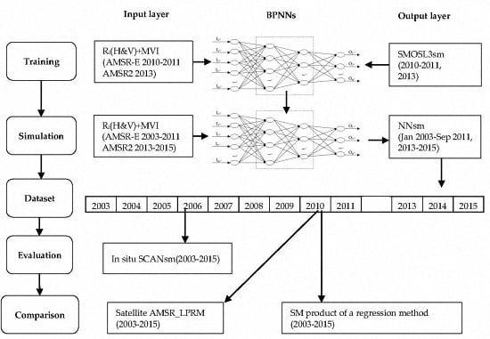
To evaluate the NNsm time series, we used in situ data from the Soil Climate Analysis Network (SCAN) [65,66]. SCAN sites are comprehensive automated weather stations that provide agricultural producers and resource managers with hourly data to monitor soil and weather conditions. Each SCAN installation can measure soil moisture and temperature at depths of 5, 10, 20 and 50 cm below ground surface. This database is available from 1 January 1996 until the present, and can provide long time series of in situ soil moisture observations that met our demands. It is an essential means of the geoscientific community for validating and improving global satellite observations and land surface models.
The sampling interval of SCAN is one hour; we use the daily average soil moisture, at a depth of 5cm, corresponding to the measurement depth of the L-band. We used 206 sites, which can provide effective data, from a total of 232 SCAN sites across the United States. We selected 15 representative SCAN sites for more detailed analysis, which covered a wide variety of land cover types, soil types, and climates [49]. The characteristics of the selected 15 sites are shown in Table 1.

2.2. Methods

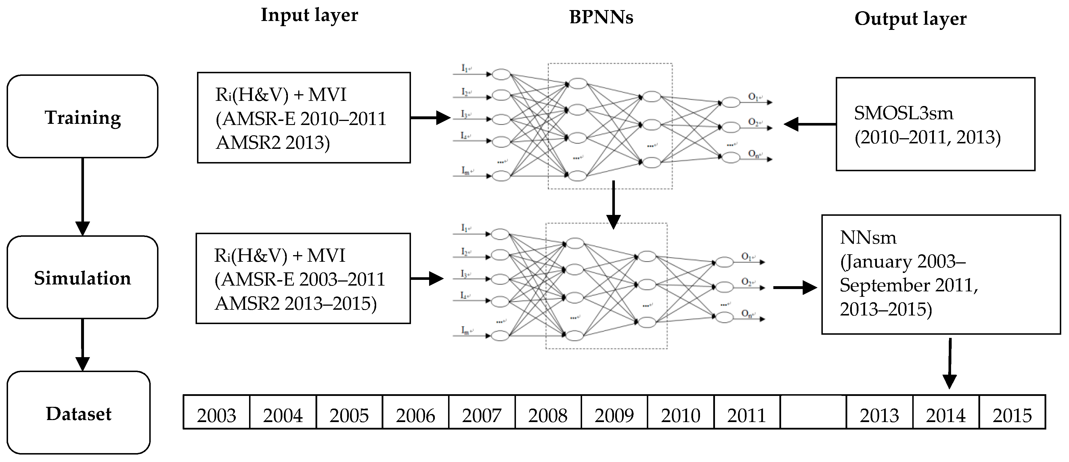
2.2.1. The BPNN Method

A neural network (NN) is a powerful nonlinear regression method. BPNN, one of the commonly-used NNs, is a type of multilayer feedforward network, in which the algorithm is trained according to error back propagation. Its learning rule is the steepest descent method, adjusting the network weights and threshold by error back propagation in order to minimize the sum of squared error of the network.
The structure of the BPNN model includes the input layer, the hidden layer, and the output layer. Our research adopted the three-layer network model with a single hidden layer. We used Matlab software to realize the training and verification of BPNN. After several tests, we selected the appropriate configurations and built the following network:
net = newff(P, T, 7, {‘tansig’, ’purelin’}, ‘trainlm’)
where P is the input vector; T is the output vector; 7 is the number of neuron nodes in the hidden layer, which is determined when the learning error does not significantly decrease with the increase of neuron nodes, after several training tests, with a small initial value of neuron nodes; ‘tansig’ is the node transfer function of the hidden layer, and it is a hyperbolic tangent sigmoid transfer function, with an arbitrary input and output, ranging from −1 to 1, which is different from the linear transfer function ‘purelin’ etc.; ‘purelin’ is the transfer function of the output layer, ‘trainlm’ is the training function that uses the Levenberg-Marquardt algorithm to estimate the training weight.
The input layer includes effective surface reflectivities (Rs) of each channel of AMSR-E/AMSR2 and the microwave vegetation index (MVI), and the output layer is the SMOSL3sm product. For the selection of key input variables in our study, we chose the Rs of the C/X/Ku/Ka/Q bands and the MVI derived from AMSR-E/AMSR2 TBs as the input layer, rather than the TBs from each channel of AMSR-E/AMSR2. Figure 1 shows the flow chart of the BPNN method.

2.2.2. Input Layer Selection

On the selection of the input layer, we start with the radiative transfer process of land surfaces. Different soil moisture contents, from dry soil to wet soil, lead to different soil dielectric constants, so the corresponding soil emissivities/reflectivities vary. The soil information is then affected by vegetation and the atmosphere and is observed by microwave sensors. The main influence factors in passive microwave retrieval of soil moisture are vegetation coverage and surface roughness. First, we adopt Rs to represent the final surface signals, which can be derived from the TB signals and the surface temperature (Ts):
R p i = 1 TB p i T s
where p is the polarization and i represents the five frequencies of AMSR-E/AMSR2. The surface temperature ( T s ) can be calculated by an empirical formula with a V polarization TB of 36.5 GHz [67]:
T s = 1.11 × TB v 36.5 15.2
Vegetation has a significant influence on total surface emissivities. The training target of the BPNN is soil moisture; in order to optimize the training relationship, we introduced the microwave vegetation index (MVI) [68] as an input for vegetation effect correction. MVI is only affected by vegetation and can express vegetation characteristics well. Previous studies have shown that MVI is related to vegetation properties and can be used for soil moisture retrieval through analytical [69] or iterative solutions [70]. In comparison to the optical vegetation indices, such as NDVI, Ratio Vegetation Index (RVI), and Leaf Area Index (LAI), MVI has the following advantages: (1) it will not be affected by the conditions of weather and lighting; (2) it will not reach saturation easily in thickly vegetated areas; and (3) it includes information about both the leafy and woody parts of vegetation, due to its greater penetration and sensitivity, while NDVI mainly responds to a thin layer of canopy. Compared to other microwave vegetation indices, such as microwave polarization difference temperature (MPDT), microwave polarization difference index (MPDI), and microwave emissivity difference vegetation index (EVDI) [71,72,73,74], MVI can remove the influence of soil background signals and only depends on vegetation properties. MVI can be derived from AMSR-E/AMSR2 TBs [68]:
MVI ( f 1 , f 2 ) = TB v ( f 2 ) TB h ( f 2 ) TB v ( f 1 ) TB h ( f 1 ) = b ( f 1 , f 2 ) × V t ( f 2 ) V t ( f 1 )
where f 1   and   f 2 are two adjacent frequencies; b is the linear coefficient of emissivity for f 1   and   f 2 ; V t is the vegetation transmission component, which is related to temperature and the overall vegetation transmissivity effect. MVI is polarization independent and is not affected by ground surface emission signals when using the ratio of polarization differences. In our study, we use the TBs of the C-band and X-band of AMSR-E/AMSR2 to calculate MVI.

2.2.3. BPNN Training

The BPNNs in Equation (1) were trained in order to determine the best relationship between the input and the output. In the training phase, we took Rs of C/X/Ku/Ka/Q bands and the MVI from AMSR-E/AMSR2 TB data as input, and used two years of SMOSL3sm data as the reference output: from 1 July 2010 to 30 June 2011, and the entire year of 2013, which coincides with the AMSR-E data and the AMSR2 data, respectively. Thus, the BPNNs were trained on each grid, over the two-year period (July 2010–June 2011, and 2013). Grids with numbers of AMSR-SMOS matching measurements (N) less than 50 were excluded.

2.2.4. Development of the NNsm Product

In the simulation phase, our input layer Rs and MVIs are derived from TBs, thus, we considered the time coverage of the AMSR-E and AMSR2 TBs. Based on the BPNNs trained in the previous step, we can develop a long-term SM dataset over 2003–2015 (except 2012) on each grid, with available AMSR-E TB from 1 January 2003 to September 2011 and AMSR2 TB from 2013 to 2015. Normally, soil moisture is not retrieved over frozen soils, thus, before the simulation, we preprocessed the TBs and TS data, removing those data where T s were lower than 273.15 K.

2.2.5. Evaluation of NNsm Product

Before application of the NNsm product, we firstly evaluate the performance of the BPNN algorithm. Because we take SMOSL3sm as a training target, we compared NNsm with SMOSL3sm during the period of the BPNN training. To evaluate long-term NNsm products, we compared NNsm products with SCAN in situ observations. The evaluation was done using the correlation coefficient (CC), the root mean square error (RMSE) and bias (Bias), defined as follows:
CC = ( x i x ¯ ) ( y i y ¯ ) ( x i x ¯ ) 2 ( y i y ¯ ) 2
where the overline indicates the mean and x i is the NNsm, y i is SMOSL3sm or SCAN in situ SM observations:
RMSE = ( x i y i ) 2 N
Bias = 1 N ( x i y i )
where N is the number of matching data.
Additionally, to better understand the similarity/dissimilarity between NNsm and other SM’s patterns with the in situ SCANsm patterns, Taylor Diagrams [75,76] were used. A Taylor Diagram provides a way of graphically summarizing how closely a pattern (or a set of patterns) matches observations. The similarity between two patterns is quantified in terms of several statistics, including their correlation (CC), their centered centered RMS difference (CRMS) and the standard deviations (SD), which are related by:
ECRMS 2 = SD 2 + 1 2 S D C C
To plot statistics of two SM products, the statistics can be normalized (and non-dimensionalized), dividing both the centered RMS difference and the SD of the two products by the SD of the in situ observations, and thus get the normalized SD (NSD) and the normalized centered RMS difference (NCRMS):
NSD = SD / SD r e f
NCRMS = CRMS / SD r e f
To understand whether SM retrievals capture the interannual variations and rainfall events, in addition to the seasonality, we compute their anomalies [18]. The anomalies (ANO) were obtained by removing the product’s seasonality SM from the original (ORI) time series:
A N O D O Y Y = O R I D O Y Y S M ¯ D O Y
where Y represents the years from 2003 to 2015, DOY means one day of the year. The seasonality S M ¯ is one time series of 366 days:
S M ¯ D O Y = ( Y = 2003 2015 O R I D O Y Y ) / N

3. Results and Analysis

3.1. BPNN Training Results

To display the training results, we compared the daily and three-day average NNsm with the corresponding reference SMOSL3sm on 2 July 2010, as shown in Figure 2. Figure 2 shows that the trained NNsm has an almost identical spatial distribution and structure with SMOSL3sm. This illustrates that the BPNN method has a good training result, and the input AMSR TB has a good nonlinear relationship with the reference SMOSL3sm.
We quantitatively evaluated the quality of the training by analyzing the agreement between the NNsm and SMOSL3sm products. The accuracy of the training results, in terms of CC, RMSE and Bias, were compared with SMOSL3sm over the training period (July 2010–June 2011, and 2013) and are shown in Figure 3.
In Figure 3a, the correlation coefficients between the reference (SMOSL3sm) and the trained SM (NNsm) are shown. The trained SM values generally correlate well with the reference SM values over most of the globe, with a global mean of CC = 0.67, and with higher values of CC (CC > 0.8) obtained over the United States, South Africa and Northwestern Africa, the south of South America, etc., and especially over Australia, where it corresponds to low to moderate vegetation coverage. Highly vegetated areas, including the Amazon and Congo rainforests, have a low correlation or failure in retrieval due to the vegetation effects. There are also areas with low vegetation coverage with poor results, such as the Arabian Peninsula. The spatial distribution of the RMSE values are plotted in Figure 3b, with a global mean of RMSE = 0.055 m3/m3. Lower RMSE values (<0.04 m3/m3) were generally distributed over arid, semi-arid, and desert regions with short and sparse vegetation or bare soil (e.g., Australia, Sahara, Southwestern United States), while high RMSE values (~0.1 m3/m3) were distributed over regions with moderate to high vegetation or alpine flora (e.g., Southeastern China, India, Southeastern Australia, Eastern United States, and locations close to the Earth’s equator). In general, the CC values are mainly moderate to high, and the RMSE values are moderate, but in an acceptable and reasonable range. Figure 3c shows the absolute value of Bias, with a magnitude of 10−3 and mean global value of Bias = −0.0005 m3/m3. The results show that the BPNN trained SM is mainly unbiased compared with the original SMOSL3sm, and it ensures the stability of the long time series of soil moisture.
In Figure 3, we can note that there is such a gap in the data such as in southern Asia. As we know, in southern Asia and the northeastern Africa, the RFI is serious. The NNs training are affected by RFI. In those areas, the NNs cannot be trained effectively or the NNs training result have a poor relationship between the input and the output, so the soil moisture cannot be retrieved correctly. The poorly retrieved NNs cause a gap in the data in southern Asia and the low correlations in northeastern Africa.
In order to better understand the accuracy of the training results, we specifically analyzed each grid that the selected SCAN sites belong to. Detailed analysis results are shown in Figure 4 and Figure 5 and Table 2. Figure 4 shows the temporal series scatterplots for the trained NNsm (red dots) versus SMOSL3sm (blue dots) over the training period (July 2010–June 2011, and 2013). As can be seen from the figures, the trend of the trained NNsm (red dots) is consistent with the trend of SMOSL3sm (blue dots), and NNsm captures the temporal dynamic of SMOSL3sm. Table 2 presents the statistical comparison between NNsm and SMOSL3sm for the training period (July 2010–June 2011, and 2013). In the analysis, we computed the statistical characteristics in terms of CC, Bias, and RMSE. Figure 5 shows the scatterplots for the trained NNsm versus SMOSL3sm and the RMSE values. In Table 2, it is obvious that the value of CC is high, ranging from 0.49 to 0.95, with an average value 0.75 of 15 selected sites and an average value 0.63 of all SCAN sites. The RMSE have an average value 0.062 m3/m3 of 15 selected sites and an average value 0.053 m3/m3 of all SCAN sites. The better values are 0.037 m3/m3 from site 2093 and 0.034 m3/m3 from site 2026; particularly, the RMSE is 0.018 m3/m3 for site 2168 for a lower dynamic range of soil moisture in an arid area. However, site 2079 has an exceptionally high RMSE value of 0.16 m3/m3. The trained net over this site cannot simulate SM well, and from the long time series in Section 3.2, the NNsm has a higher dynamic range than that of SCAN sm. The value of Bias has a magnitude of 10−3 and better ones can be 10−4 from site 2026 and site 2075. The unbiased trained results ensure the stability and consistency of the NNsm products. This indicates that the trained results are unbiased compared with original soil moisture, which is the most important factor to ensure the stability and consistency of the long time series soil moisture products.

3.2. NNsm Products and Evaluation

We further undertook assessments to evaluate the performance of the long-term NNsm products over the period of 2003 to 2015 (except 2012) with the in situ observations of the SCAN sites. The satellite standard SM products of AMSR-E/AMSR2 (AMSRsm) from NSIDC and JAXA were also added as a reference. The evaluations were done by plotting time series, and in terms of CC, RMSE and Bias, as shown in Figure 6, Figure 7, Figure 8 and Figure 9 and Table 3 (left part).
Figure 6, Figure 7, Figure 8 and Figure 9 show the temporal series scatterplots (upper panel) and anomaly time series (lower panel) for SCANsm (red line), NNsm (blue dots) and AMSRsm (green diamonds) over a long time period (2003–2015). Table 3 (left) shows the CC, RMSE and Bias of the selected SCAN sites and all SCAN sites. For the results of NNsm vs. SCANsm, the CC has a mean value 0.52 of 15 selected sites and 0.43 of all SCAN sites, ranging from 0.21 to 0.71. The RMSE has a mean value 0.084 m3/m3 for 15 selected sites and 0.078 m3/m3 for all SCAN sites. The value of Bias has a magnitude of 10−3 and an average value −0.004 of all SCAN sites. From the time series plots, it is evident that the majority of the SCAN sites have a good consistency between NNsm and SCANsm, but several SCAN sites overestimate or underestimate the soil moisture. The performance of NNsm is superior to that of AMSRsm. AMSRsm from NSIDC and JAXA underestimate soil moisture significantly and has a little variation range.
For anomaly time series, after removing the contribution of seasonal cycle, the mean value of CC is lower than that of origin time series, while the mean value of RMSE decreases, as shown in Table 2. It means that the seasonal cycles make a considerable contribution to the value of origin CC. In addition to the seasonal cycles, NNsm weakly capture the interannual variations and the rainfall events. In contrast, after removing the contribution of seasonal cycle, the AMSRsm hardly has a fluctuation, based on the little variation range of original time series. It means that AMSRsm can weakly capture the seasonal cycles and cannot capture the interannual variations and the rainfall events. Detailed analysis is presented by dividing these sites into three categories: (1) sites with strong interannual variations; (2) sites with weak interannual variations; and (3) sites in semi-arid areas.

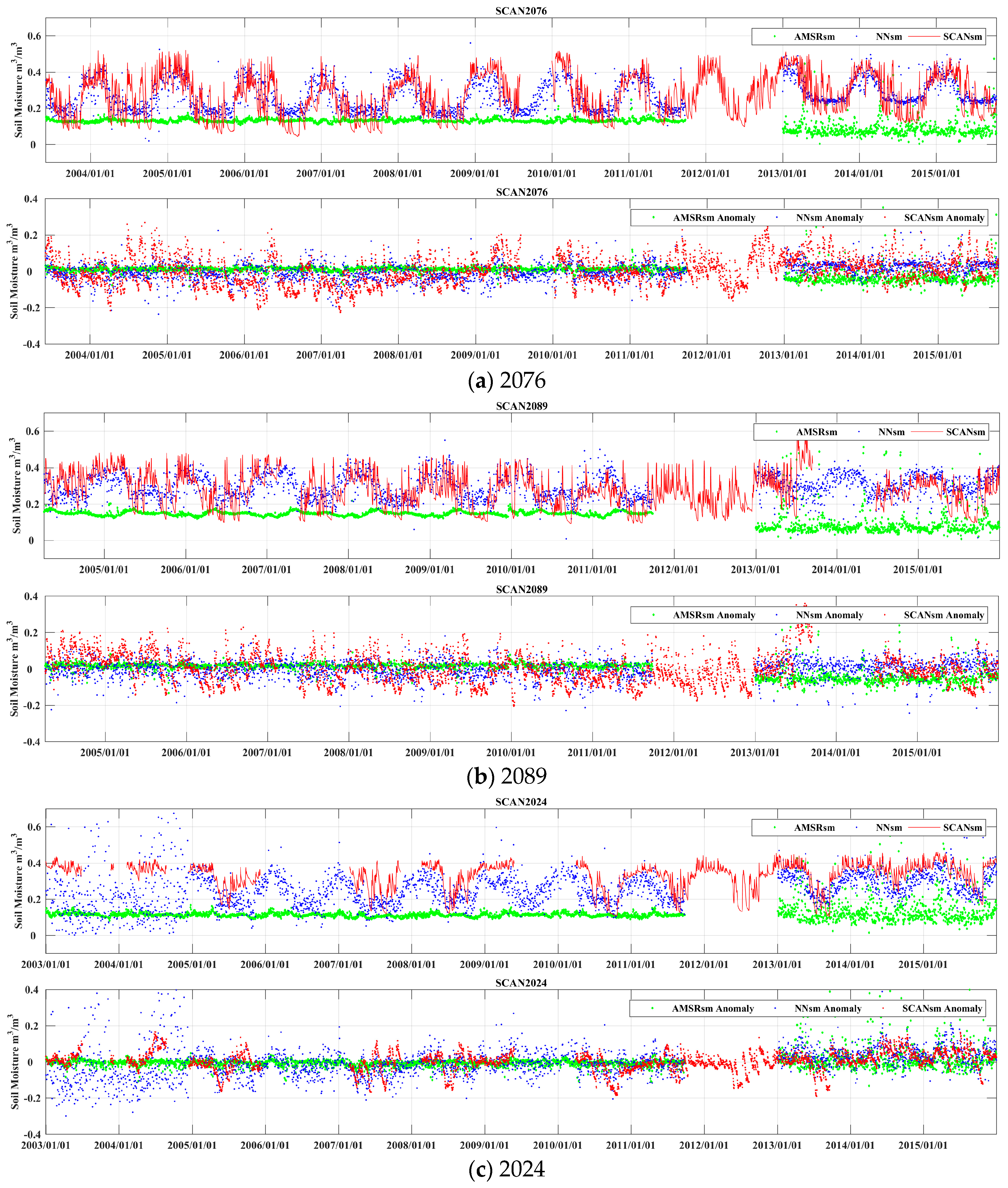
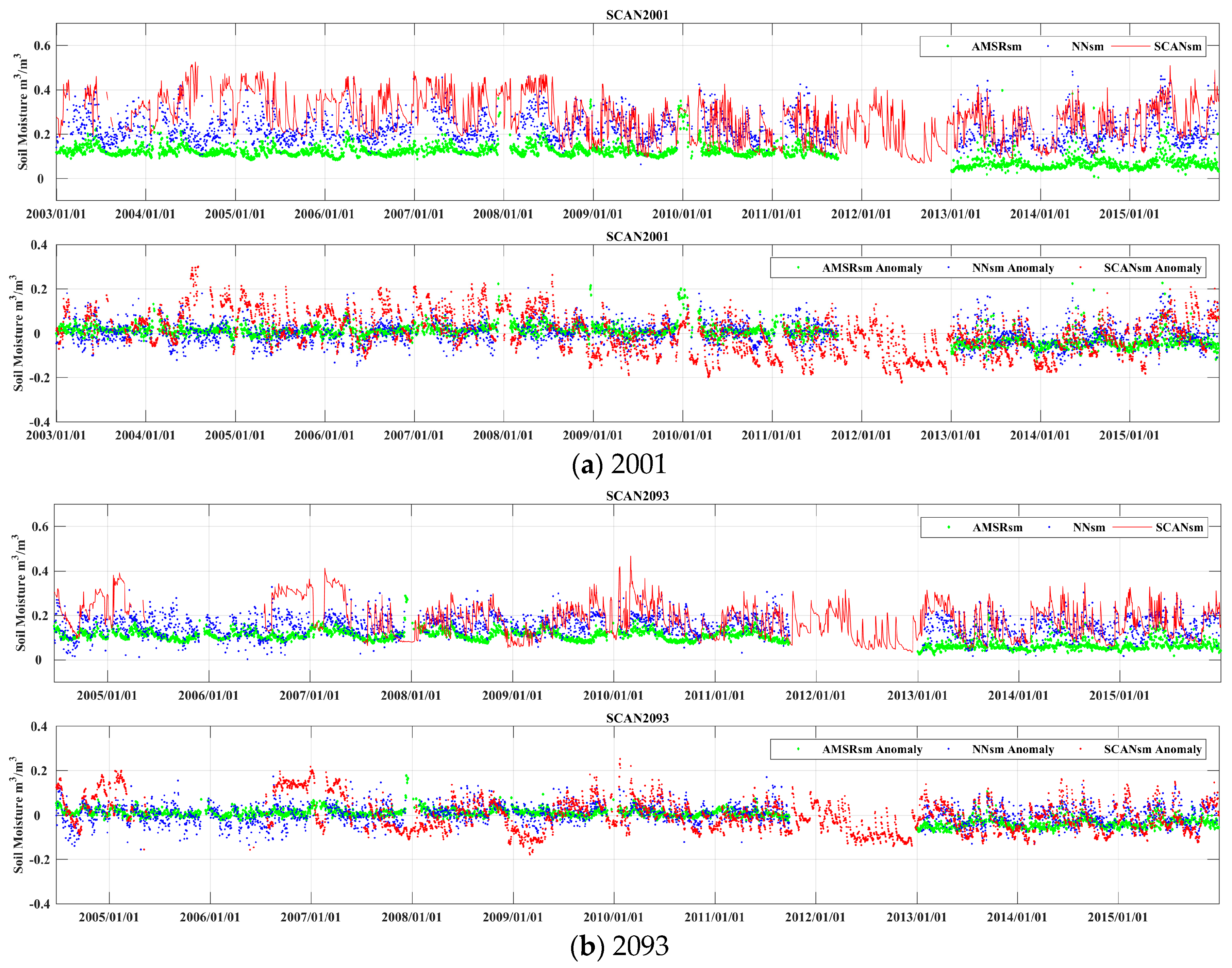
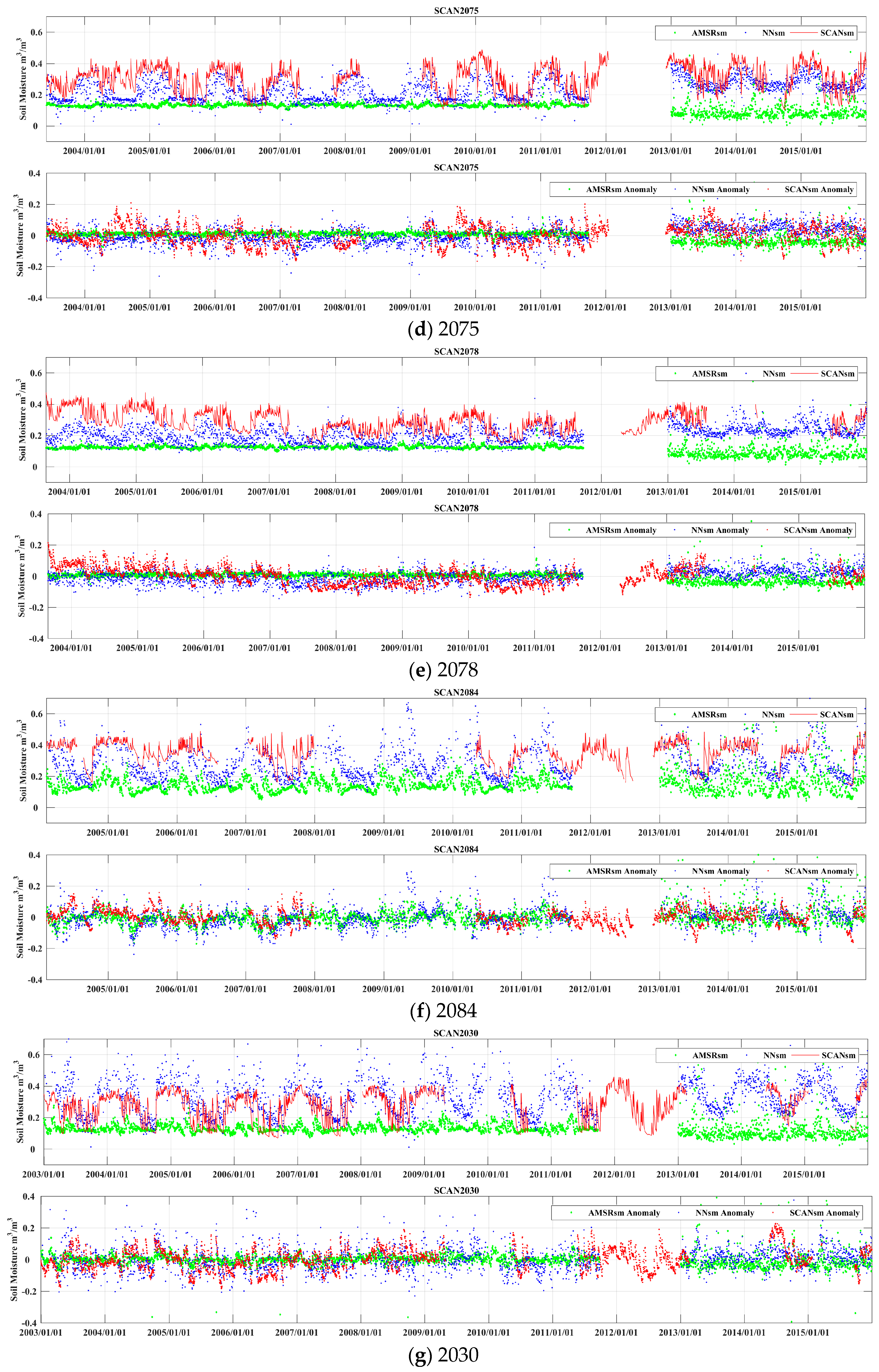
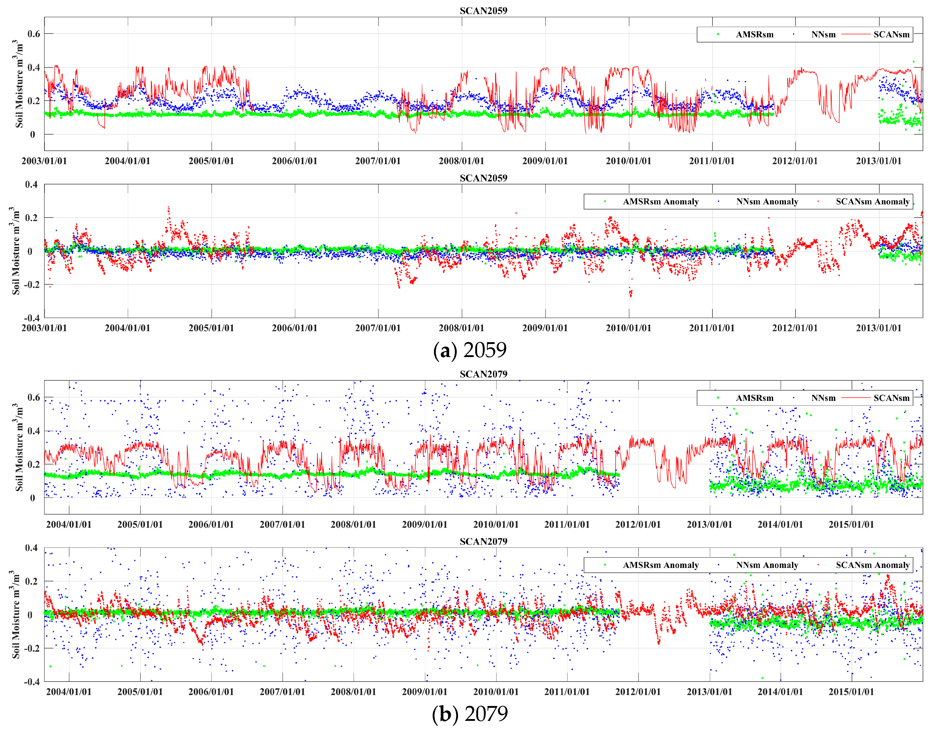
3.2.1. Sites with Strong Interannual Variations

Figure 3 shows the time series and anomaly time series for seven SCAN sites from Table 3. From these time series figures, it is obvious that the NNsm can capture the dynamic variety of SCAN in situ soil moisture well, and the interannual variation of NNsm is noteworthy. Relatively speaking, the fluctuation range of SCANsm is bigger than that of NNsm. Furthermore, there are problems in the consistency and the continuity of the soil moisture between AMSR-E and AMSR2. The most consistent sites are SCAN site 2076 and site 2089, with almost no bias. However, for SCAN site 2024, site 2075, site 2078, and site 2084, the NNsm underestimated the soil moisture by 7%, 6%, 8%, and 6%, respectively. Especially, for site 2078 and site 2084, the NNsm have obviously been underestimated from 2003 to 2006. For site 2030, the NNsm overestimated soil moisture, particularly in the peak area of interannual soil moisture variability. For anomaly time series, after removing the contribution of seasonal cycle NNsm weakly capture the interannual variations and the rainfall events, while AMSRsm cannot capture the interannual variations and the rainfall events.
Figure 7 shows the time series and anomaly time series for two SCAN sites from Table 3. From these time series figures, it is obvious that NNsm can capture the interannual dynamic variety of in situ soil moisture well, but the dynamic ranges have some differences.
Over site 2059, the dynamic range of NNsm is lower than that of SCAN in situ soil moisture. From the trained time series plot of site 2059 in Figure 4, the reference SMOSL3sm is distributed in the range of 0.1–0.3 m3/m3, so the trained NNsm is also distributed in this range. However, the SCANsm in this site range from 0 to 0.4 m3/m3. Therefore, the range difference of site 2059 is mainly derived from the difference between the reference SMOSL3sm and the in situ SCANsm.
Over site 2079, the dynamic range of NNsm is higher than that of in situ SCANsm. Land cover of this site is deciduous broadleaf forest, while around 76% of the site is a cropland/natural vegetation mosaic. The soil moisture in crop lands has a higher variety in range than that in forest areas. Therefore, NNsm has a higher dynamic range than in situ site soil moisture.
For anomaly time series, after removing the contribution of seasonal cycle, NNsm still has a smaller range and a bigger range than SCANsm, over site 2059 and 2079 respectively. AMSRsm series is almost a flat line, and cannot capture the interannual variations and the rainfall events.

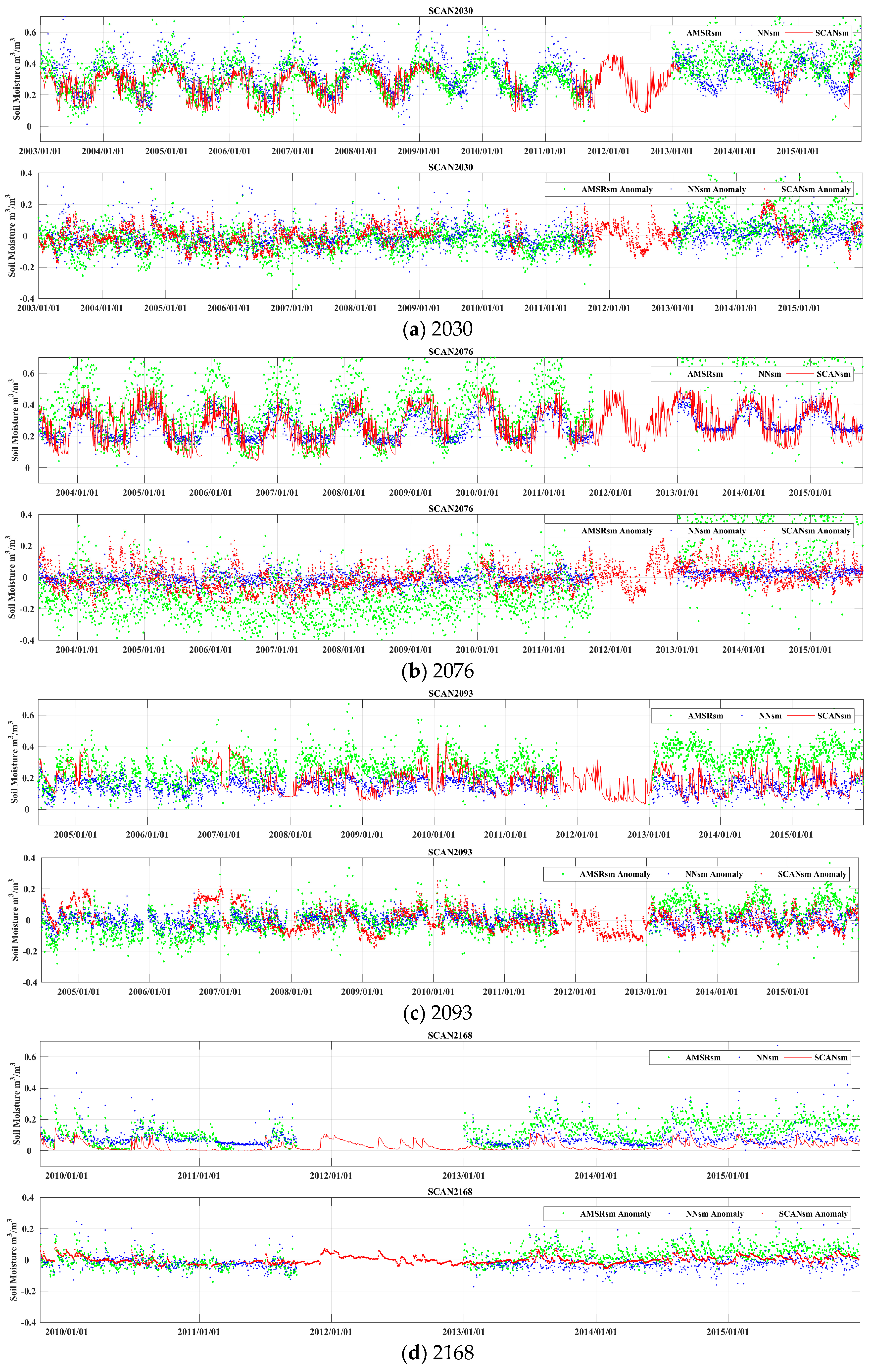
3.2.2. Sites with Weak Interannual Variations

Over site 2001 and site 2093, shown in Figure 8, NNsm is roughly in agreement with SCANsm. However, the interannual variation of soil moisture is weaker. AMSRsm underestimated the soil moisture. Through the analysis of the land cover, we found the reason for this.
The land cover of these two sites is cropland, and, around the two sites, 72% land cover of site 2001 and 84% land cover of site 2093 are croplands. Crops are short vegetation, so the soil moisture changes faster. After rain or irrigation, soil moisture content will decrease rapidly. The corresponding change trend of soil moisture over these two sites is falls rapidly after rising. Additionally, when SCANsm is higher than the overall SM level from 2003 to 2007, and is higher than that in the training period, NNsm has obvious underestimations in soil moisture.

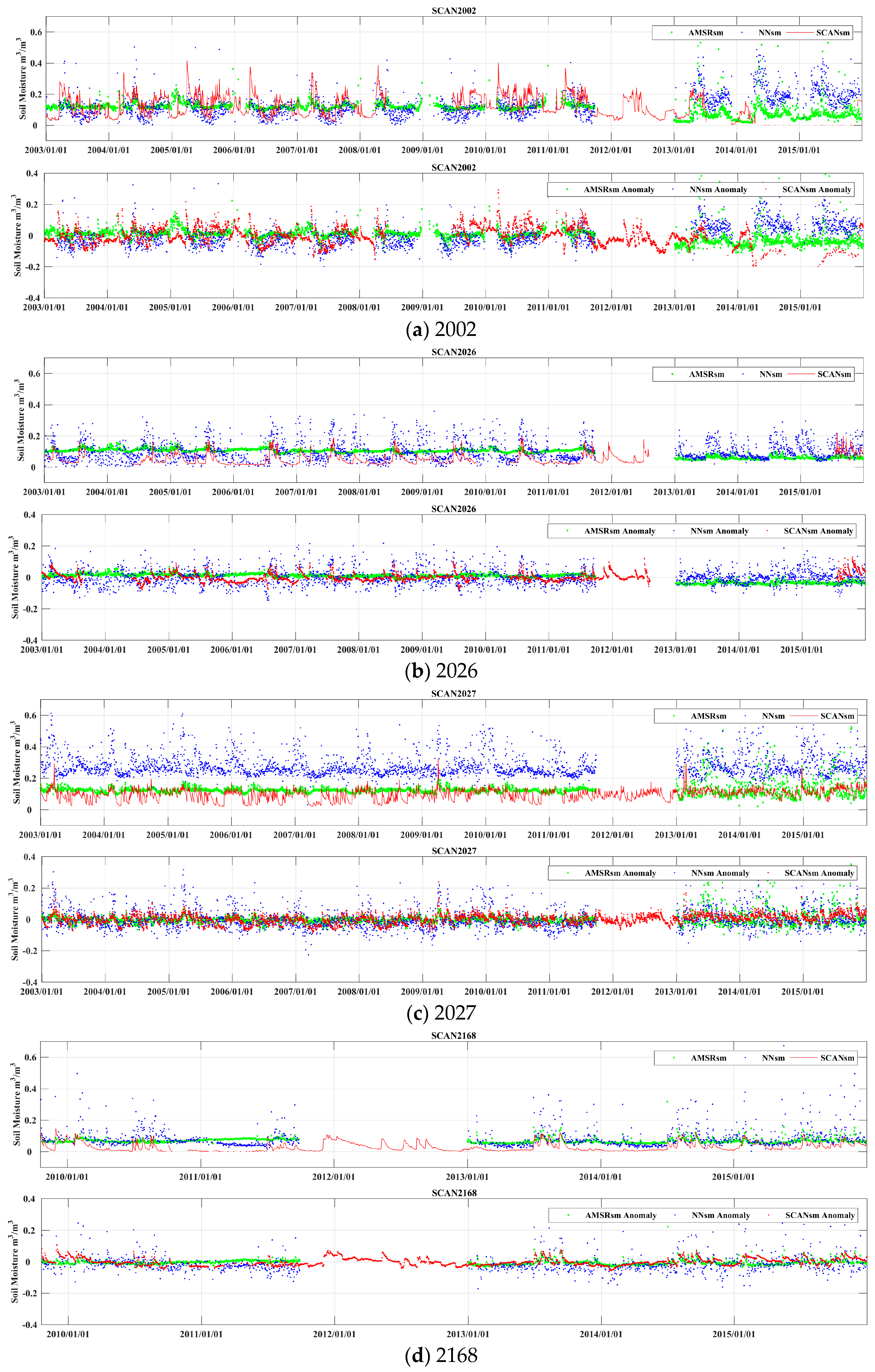
3.2.3. Sites in Semi-Arid Areas

Figure 9 shows a time series of soil moisture over four sites: Site 2002, site 2026, site 2027, and site 2168, which are located in semi-arid areas. Over these four sites, the soil moisture level is not high, and basically remains below 0.2 m3/m3. NNsm overestimates the soil moisture over site 2026, site 2027, and site 2168, particularly in the drier period, while NNsm underestimated the soil moisture of site 2002. The main landcover types around these sites are croplands, cropland/natural vegetation mosaic, and grassland and open shrublands. Around site 2027, 88% is croplands and cropland/natural vegetation mosaic. A total of 96% of the surface of site 2168 is shrubland. For site 2002, most surfaces are croplands. The surface of site 2026 is 48% grasslands and 52% open shrublands. Thus, the soil moisture of these sites changes faster.
From the trained time series plots of site 2026, site 2027, and site 2168, in Figure 4, the reference SMOSL3sm distributed at around 0.1 m3/m3, 0.1–0.5 m3/m3, and 0.1 m3/m3, so the trained NNsm also distributed in these ranges, respectively. However, the SCANsm from site 2026 and site 2168 were almost 0 m3/m3 in the drier period, and the SCANsm of site 2027 ranges from 0 to 0.2 m3/m3, which are distinctly lower than the level of in situ observations. Therefore, the differences on these sites are mainly derived from the differences between the reference SMOSL3sm and the in situ SCANsm.
Compared with SCANsm and NNsm, we can clearly find that AMSRsm has an overestimation of soil moisture. Additionally, soil moisture from AMSR-E and AMSR2 have poor consistency and continuity, especially for AMSR2 soil moisture from 2013 to 2015 over site 2002 and site 2027, while NNsm has a better consistency and continuity.
For anomaly time series over site 2027, the total shift between NNsm and SCANsm was removed, and the NNsm still overestimates the soil moisture. The NNSm can slightly capture the interannual variations.
The disagreement between the satellite derived NNsm and the in situ observations may be caused by several factors. First, satellite-derived soil moisture represents the spatial mean value within a satellite footprint, while the in situ soil moisture observations are point measurements. The scaling difference between the point observations and the surface observations will lead to a disagreement, especially in terms of RMSE and Bias [71]. In addition, the soil moisture derived from satellite data may have a different representative depth with that observed from in situ sites. The satellite-derived soil moisture may dry more rapidly after rainfall events or irrigation than that of in situ sites. Moreover, the heterogeneity in the satellite footprint will lead to the difference between the satellite grids and the in situ sites. For example, soil moisture will differ and change rapidly with cropland land cover of a site than that of a footprint with 80% forest. Despite all the above-mentioned impacting factors, NNsm reproduced the soil moisture variability and changing trends without drifts in the long-term data record well, which is essential for climate analyses.

4. Comparison and Discussion

To clarify the advantages of our retrieval results, we further discuss our soil moisture products (NNsm) by comparing them with other long-term soil moisture products, generated using alternative methods: (a) AMSR-E/2 soil moisture products generated using the same algorithm, the LPRM (Land Parameter Retrieval Model) algorithm (AMSR_LPRM hereafter), through cross-calibration; and (b) AMSR-E soil moisture retrievals through a regression method (Reg_sm hereafter) with the target reference of SMOSL3sm.

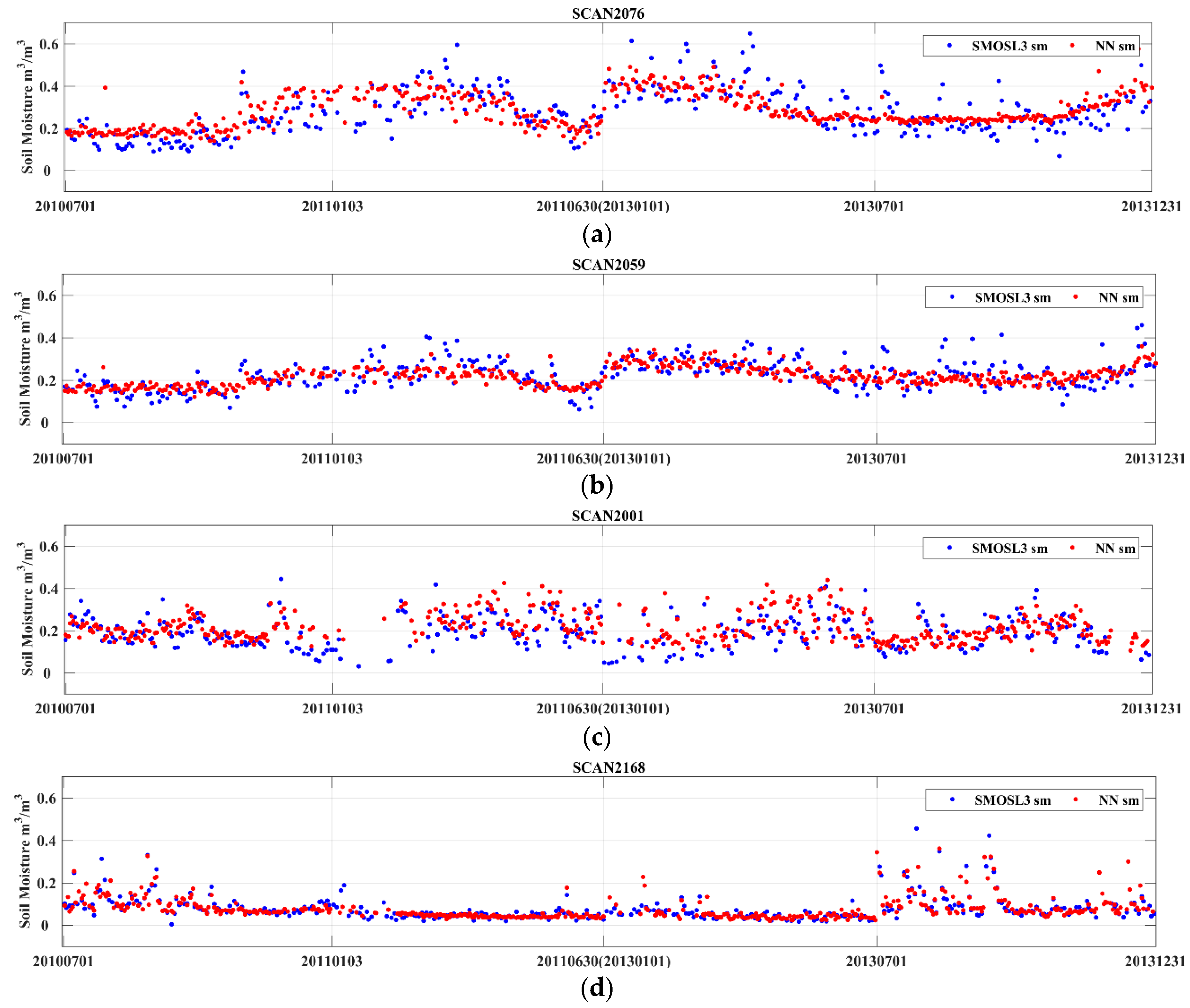
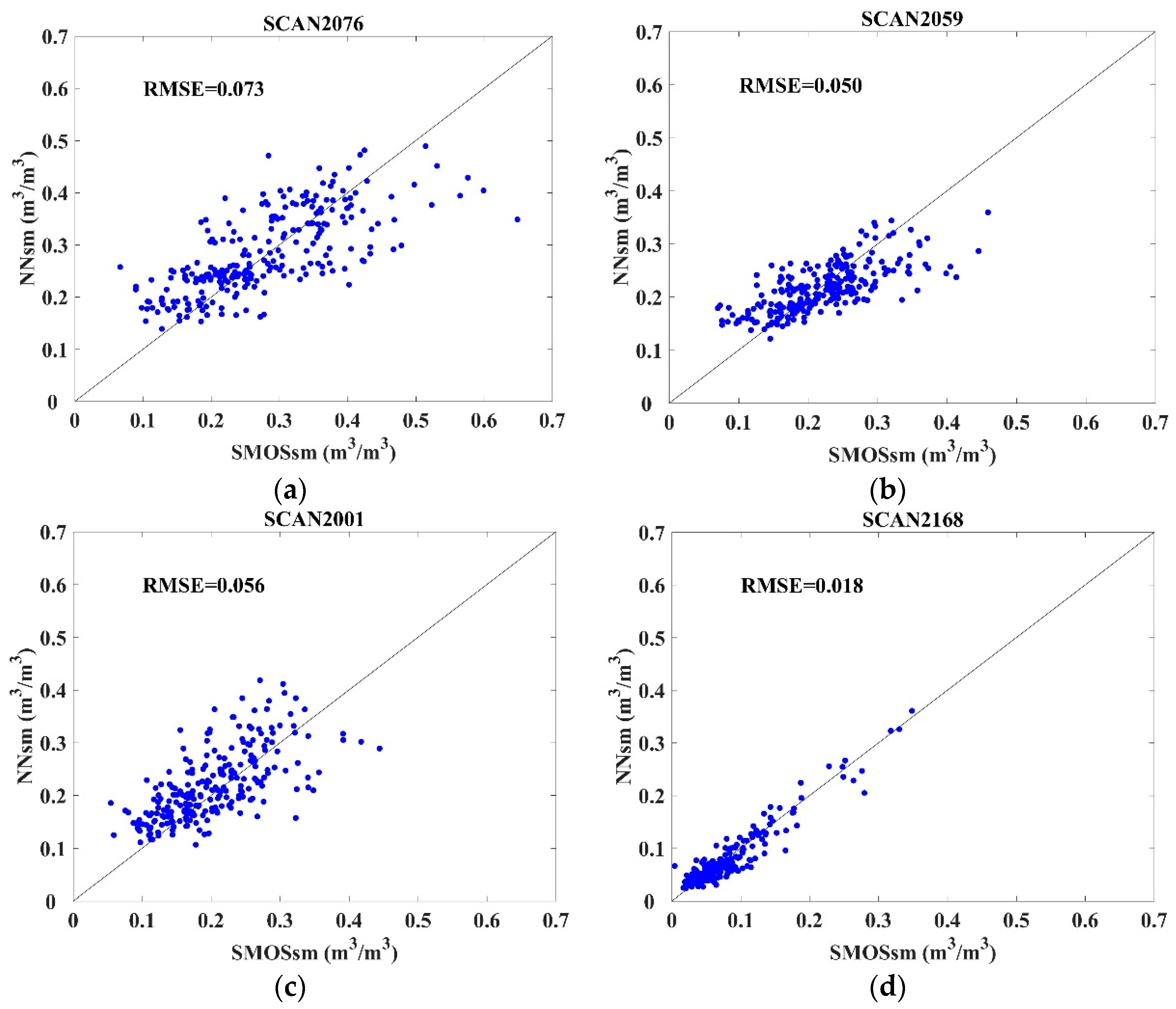
4.1. Comparing with Satellite Products

In Section 3, we compared NNsm with the reference SMOSL3sm, in situ SCANsm, and AMSRsm. It turns out that NNsm has a high consistency and accuracies relative to the reference. However, the AMSRsm from NSIDC and JAXA underestimate SM significantly. In this section, we discuss the performance of NNsm by comparing it with AMSR-E and AMSR2 soil moisture products (we call it AMSR_LPRM), generated by the same algorithm, namely the LPRM algorithm. These long time-series datasets are from two similar sensors, namely AMSR-E and AMSR2 satellite sensors, and further more they are retrieved both from the LPRM algorithm and are from one dataset, so we treated them as one long time-series datasets. We average the statistical results of the 15 selected sites, as shown in Table 3.
From the point of view of the time series (upper panel) and anomaly time series (lower panel) shown in Figure 10, it is obvious that NNsm is more consistent and continuous with SCANsm than the performance of AMSR-LPRM. AMSR_LPRM overestimate soil moisture over these sites. Additionally, the soil moisture from AMSR-E and AMSR2 are not consistent over these sites. Some panels show a shift in soil moisture in the AMSR-E period compared to the AMSR-2 period that could be explained by not accounting for possible bias between the LPRM datasets. Over site 2076, there is a big shift between the AMSR-E and AMSR2 data, so after anomaly process, AMSR-E underestimates the soil moisture and the AMSR2 overestimate the soil moisture. With respect to accuracy, NNsm has an average value of CC = 0.52 for 15 selected sites and CC = 0.43 for all sites; and NNsm has a mean value of RMSE = 0.084 for 15 selected sites and RMSE = 0.078 for all sites. These statistics of NNsm is more accurate than that of AMSR_LPRM, whether the time series or the anomaly time series.
Furthermore, the Taylor diagram is presented to display statistical comparison between NNsm (blue dots) and AMSRsm/AMSR_LPRM (green dots) with the in situ SCANsm (red dot) over the long time period (2003–2015) for all SCAN sites, as shown in Figure 11. In general, the dots (sites) are unevenly distributed in the Taylor diagram for both NNsm and AMSRsm/AMSR_LPRM, meaning that their accuracy varies from one site to another. For the left panel, the NSDs of AMSRsm are much less than the one unit of normalized NSD, indicating a little variability of AMSRsm. For the right panel, the NSDs of AMSR_LPRM are much larger than the one unit of normalized NSD, indicating a larger variability of AMSR_LPRM. While the NSD of NNsm are always around the arc of one unit, compared with that of AMSRsm/AMSR_LPRM. As shown in the diagrams, the NNsm has a slightly higher CC with SCANsm than that of AMSRsm/AMSR_LPRM, meaning that these three products have very comparable correlation with SCANsm. Additionally, most blue dots are within the arc of one unit of CRMS, indicating that NNsm matches SCANsm more.

4.2. Comparing with a Regression Method

As mentioned in the Introduction Section, Al-Yaari et al. [39] used a regression approach to retrieve global time series soil moisture datasets, with SMOSL3sm as a training reference target and AMSR-E TB as training input. We compared results NNsm with Reg_sm of the algorithm used by Al-Yaari. The comparative results are listed in Table 4 for the training and simulation period.
In the training period, compared with the reference SMOSL3sm, NNsm has a slightly higher CC 0.67 than 0.60 of Reg_sm, and NNsm has a slightly lower RMSE 0.055 m3/m3 than 0.057 m3/m3 of Reg_sm. By the statistical comparisons, we can see that our NNsm has a better training result than the Reg_sm. Moreover, the input of NNsm includes TBs from AMSR-E and AMSR2, while the input of Reg_sm is only AMSR-E TB. It makes it possible to derive continuous and longer soil moisture dataset from AMSR-E and AMSR2 TB in the next simulation step.
In the simulation period, from an accuracy perspective against SCANsm, NNsm has a slightly higher CC 0.52 than 0.49 of Reg_sm. However, the two algorithms have nearly equal RMSE when compared with in situ SCANsm. For the long-term dataset, the NNsm can simulate soil moisture from 2013 to 2015 based on AMSR-E/AMSR2 TBs, longer than the dataset from Reg_sm.

5. Conclusions

This study investigates the feasibility of a BPNN method to build a long time-term soil moisture time series using SMOSL3sm products and AMSR-E/AMSR2 TB observations. First, the BPNNs on every grid were trained using SMOSL3sm products as a training target, and we took reflectivity (R) and the MVI from AMSR-E/AMSR2 TB observations during July 2010–June 2011 and the entire year of 2013 as inputs. With these BPNNs, we built long time series of global soil moisture from 2003 to 2015, using AMSR-E TB in 2003–2011 and AMSR2 TB in 2013–2015.
We evaluated the quality of the training step over the training period (July 2010–June 2011, and 2013), and it achieved a good agreement between the NNsm and SMOSL3sm products, with a mean global value of CC = 0.67, RMSE = 0.055 m3/m3 and Bias = −0.0005 m3/m3. A specific analysis on selected SCAN sites shows that the trend of the trained NNsm is consistent with that of SMOSL3sm, with a high CC value. These results ensure the following step of building a long time series of soil moisture.
The long time series and anomaly time series of NNsm were evaluated against in situ SCANsm observations. It turns out that our result NNsm has a high consistency and accuracy with reference SMOSL3sm and the in situ SCANsm, and captured the temporal dynamics of soil moisture, with CC = 0.52, RMSE = 0.084 m3/m3 and a Bias with a magnitude of 10−3. Over most of the SCAN sites, NNsm well captures the in situ SCANsm and has strong seasonal and interannual variations. However, in some SCAN sites, although our method can capture the interannual dynamic variety well, there are some differences in the dynamic ranges between NNsm and SCANsm. This can be mainly explained by two factors, in which one is the differences between the reference SMOSL3sm and the in situ SCANsm, and the other is the heterogeneity in the satellite footprint. The soil moisture of some sites has weak interannual variations. Through our analyses we found that the land cover is mainly croplands. Thus, influenced by irrigation in these areas, soil moisture changes faster and has no obvious interannual variations. In some semi-arid sites, NNsm has overestimated or underestimated soil moisture. There are differences between the reference SMOSL3sm and the in situ SCANsm, which is the reason for overestimations or underestimations.
To further evaluate the accuracy and state the advantages of NNsm, we compared it with AMSR_LPRM products and a regression method. Comparative results show that NNsm is more consistent and continuous with SCANsm than the performances of AMSR_LPRM and Reg_sm. NNsm has significant advantages relative to the regression method, with a higher accuracy and longer time series.
For improvement and further research, we wish to continue the following work: (1) for the improvement of our BPNN method, we can test different combinations of Rs and MVI. For example, we can use low or high frequency bands of Rs and MVI, as we used all frequencies in this study, which may not be the optimal input combination for BPNN training; (2) Another direction is to train BPNNs for future WCOM. Because WCOM will have no overlapping data with AMSR-E data, we can train BPNNs using only the AMSR2 data and apply the BPNNs to cross-calibrated AMSR2 and AMSRE data.
In conclusion, through BPNNs training, this study provides a promising method to build long time series of global soil moisture products. The BPNN method can produce surface soil moisture in terms of absolute values and temporal variations. In addition, the BPNN method is independent of various ancillary data, and only relies on the reference SMOS data. This method can be applied in other satellite missions, such as SMAP and future WCOM satellite mission, so long as they have an overlap period with AMSR-E/AMSR2 observations.

Acknowledgments

This work was supported in part by the National Key Basic Research Program (2015CB953701), Key Research Program of Frontier Sciences, CAS (Grant No. QYZDY-SSW-DQC011), International S&T Cooperation Program of China (2016YFE0117300), the National Natural Science Foundation of China (41371354, 41301396) and the Youth Innovation Promotion Association (No. 2016061). The authors would like to acknowledge CATDS for providing the SMOS L3 datasets. The authors thank the NSIDC and the JAXA for providing the AMSR-E/AMSR2 TB and SM data, the NASA for providing the AMSRsm products and the ISMN for providing SCAN observations.

Author Contributions

Jiancheng Shi and Panpan Yao conceived and designed the work; Panpan Yao performed the experiments; Panpan Yao and Tianjie Zhao analyzed the data and wrote the manuscript; Hui Lu and Amen Al-Yaari provided useful suggestions, and modified the manuscript.

Conflicts of Interest

The authors declare no conflicts of interest.

References

  1. Entekhabi, D.; Njoku, E.G.; O’Neill, P.E.; Kellogg, K.H.; Crow, W.T.; Edelstein, W.N.; Entin, J.K.; Goodman, S.D.; Jackson, T.J.; Johnson, J.; et al. The soil moisture active passive (SMAP) mission. Proc. IEEE 2010, 98, 704–716. [Google Scholar] [CrossRef]
  2. Wigneron, J.P.; Calvet, J.C.; Pellarin, T.; Van de Griend, A.A.; Berger, M.; Ferrazzoli, P. Retrieving near-surface soil moisture from microwave radiometric observations: Current status and future plans. Remote Sens. Environ. 2003, 85, 489–506. [Google Scholar] [CrossRef]
  3. Fang, B.; Lakshmi, V. Soil moisture at watershed scale: Remote sensing techniques. J. Hydrol. 2014, 516, 258–272. [Google Scholar] [CrossRef]
  4. Fang, B. Disaggregation of Passive Microwave Soil Moisture for Use in Watershed Hydrology Applications. Ph.D. Thesis, University of South Carolina, Columbia, SC, USA, 2015. [Google Scholar]
  5. Su, Z.; Yacob, A.; Wen, J.; Roerink, G.; He, Y.; Gao, B.; Boogaard, H.; van Diepen, C. Assessing relative soil moisture with remote sensing data: Theory, experimental validation, and application to drought monitoring over the North China Plain. Phys. Chem. Earth Parts A/B/C 2003, 28, 89–101. [Google Scholar] [CrossRef]
  6. Kerr, Y.H.; Waldteufel, P.; Wigneron, J.P.; Delwart, S.; Cabot, F.; Boutin, J.; Escorihuela, M.J.; Font, J.; Reul, N.; Gruhier, C.; et al. The SMOS mission: New tool for monitoring key elements of the global water cycle. Proc. IEEE 2010, 98, 666–687. [Google Scholar] [CrossRef] [Green Version]
  7. Zhang, D.; Anthes, R.A. A high-resolution model of the planetary boundary layer-sensitivity tests and comparisons with SESAME-79 data. J. Appl. Meteorol. 1982, 21, 1594–1609. [Google Scholar] [CrossRef]
  8. Houser, P.R.; Shuttleworth, W.J.; Famiglietti, J.S.; Gupta, H.V.; Syed, K.H.; Goodrich, D.C. Integration of soil moisture remote sensing and hydrologic modeling using data assimilation. Water Resour. Res. 1998, 34, 3405–3420. [Google Scholar] [CrossRef]
  9. Shi, J.; Dong, X.; Zhao, T.; Du, J.; Jiang, L.; Du, Y.; Liu, H.; Wang, Z.; Ji, D.; Xiong, C. WCOM: The science scenario and objectives of a global water cycle observation mission. In Proceedings of the IEEE International Geoscience and Remote Sensing Symposium (IGARSS), Quebec City, QC, Canada, 13–18 July 2014.
  10. Dong, X.; Liu, H.; Wang, Z.; Shi, J.; Zhao, T. WCOM: The mission concept and payloads of a global water cycle observation mission. In Proceedings of the IEEE International Geoscience and Remote Sensing Symposium (IGARSS), Quebec City, QC, Canada, 13–18 July 2014.
  11. Schmugge, T.; Wilheit, T.; Webster, W., Jr.; Gloerson, P. Remote sensing of soil moisture with microwave radiometers. J. Geophys. Res. 1974, 79, 317–323. [Google Scholar] [CrossRef]
  12. Walker, J.P.; Houser, P.R. Requirements of a global near-surface soil moisture satellite mission: Accuracy, repeat time, and spatial resolution. Adv. Water Resour. 2004, 27, 785–801. [Google Scholar] [CrossRef]
  13. Gloersen, P.; Hardis, L. The scanning multichannel microwave radiometer (SMMR) experiment. In Its the Nimbus 7 User’s Guide; SEE N79-20148 11-12; NASA/Goddard Space Flight Center: Greenbelt, MD, USA, 1978. [Google Scholar]
  14. Ashcroft, P.; Wentz, F. Algorithm Theoretical Basis Document: AMSR Level 2A Algorithm; Robotics: Science & Systems: Santa Rosa, CA, USA, 2000. [Google Scholar]
  15. Njoku, E.G.; Jackson, T.J.; Lakshmi, V.; Chan, T.K.; Nghiem, S.V. Soil moisture retrieval from AMSR-E. IEEE Trans. Geosci. Remote Sens. 2003, 41, 215–229. [Google Scholar] [CrossRef]
  16. Le Vine, D.M.; Lagerloef, G.S.; Colomb, F.R.; Yueh, S.H.; Pellerano, F.A. Aquarius: An instrument to monitor sea surface salinity from space. IEEE Trans. Geosci. Remote Sens. 2007, 45, 2040–2050. [Google Scholar] [CrossRef]
  17. Bindlish, R.; Jackson, T.; Cosh, M.; Zhao, T.; O'Neill, P. Global soil moisture from the Aquarius/SAC-D satellite: Description and initial assessment. IEEE Geosci. Remote Sens. Lett. 2015, 12, 923–927. [Google Scholar] [CrossRef]
  18. Liu, Y.Y.; Dorigo, W.A.; Parinussa, R.M.; de Jeu, R.A.; Wagner, W.; McCabe, M.F.; Evans, J.P.; Van Dijk, A.I.J.M. Trend-preserving blending of passive and active microwave soil moisture retrievals. Remote Sens. Environ. 2012, 123, 280–297. [Google Scholar] [CrossRef]
  19. Baghdadi, N.; Gaultier, S.; King, C. Retrieving surface roughness and soil moisture from synthetic aperture radar (SAR) data using neural networks. Can. J. Remote Sens. 2002, 28, 701–711. [Google Scholar] [CrossRef]
  20. Jiang, H.; Cotton, W.R. Soil moisture estimation using an artificial neural network: A feasibility study. Can. J. Remote Sens. 2004, 30, 827–839. [Google Scholar] [CrossRef]
  21. Paloscia, S.; Pampaloni, P.; Pettinato, S.; Santi, E. A comparison of algorithms for retrieving soil moisture from ENVISAT/ASAR images. IEEE Trans. Geosci. Remote Sens. 2008, 46, 3274–3284. [Google Scholar] [CrossRef]
  22. Pierdicca, N.; Castracane, P.; Pulvirenti, L. Inversion of electromagnetic models for bare soil parameter estimation from multifrequency polarimetric SAR data. Sensors 2008, 8, 8181–8200. [Google Scholar] [CrossRef] [PubMed]
  23. Paloscia, S.; Pettinato, S.; Santi, E.; Notarnicola, C.; Pasolli, L.; Reppucci, A. Soil moisture mapping using Sentinel-1 images: Algorithm and preliminary validation. Remote Sens. Environ. 2013, 134, 234–248. [Google Scholar] [CrossRef]
  24. Gruber, A.; Paloscia, S.; Santi, E.; Notarnicola, C.; Pasolli, L.; Smolander, T.; Pulliainen, J.; Mittelbach, H.; Dorigo, W.; Wagner, W. Performance inter-comparison of soil moisture retrieval models for the MetOp-A ASCAT instrument. In Proceedings of the IEEE International Geoscience and Remote Sensing Symposium (IGARSS), Quebec City, QC, Canada, 13–18 July 2014; pp. 2455–2458.
  25. Paloscia, S.; Pettinato, S.; Santi, E.; Huttunen, M.; Silander, J.; Vehvilainen, B. Soil moisture maps from ENVISAT/ASAR images in a Finland area obtained by using an algorithm based on Neural Networks. In Proceedings of the Geophysical Research Abstracts, Vienna, Austria, 2–7 April 2006.
  26. Liu, S.F.; Liou, Y.A.; Wang, W.J.; Wigneron, J.P.; Lee, J.B. Retrieval of crop biomass and soil moisture from measured 1.4 and 10.65 GHz brightness temperatures. IEEE Trans. Geosci. Remote Sens. 2002, 40, 1260–1268. [Google Scholar]
  27. Del Frate, F.; Ferrazzoli, P.; Schiavon, G. Retrieving soil moisture and agricultural variables by microwave radiometry using neural networks. Remote Sens. Environ. 2003, 84, 174–183. [Google Scholar] [CrossRef]
  28. Chai, S.S.; Walker, J.P.; Makarynskyy, O.; Kuhn, M.; Veenendaal, B.; West, G. Use of soil moisture variability in artificial neural network retrieval of soil moisture. Remote Sens. 2009, 2, 166–190. [Google Scholar] [CrossRef]
  29. Liou, Y.A.; Liu, S.F.; Wang, W.J. Retrieving soil moisture from simulated brightness temperatures by a neural network. IEEE Trans. Geosci. Remote Sens. 2001, 39, 1662–1672. [Google Scholar]
  30. Santi, E.; Pettinato, S.; Paloscia, S.; Pampaloni, P.; Macelloni, G.; Brogioni, M. An algorithm for generating soil moisture and snow depth maps from microwave spaceborne radiometers: HydroAlgo. Hydrol. Earth Syst. Sci. 2012, 16, 3659–3676. [Google Scholar] [CrossRef]
  31. Notarnicola, C.; Angiulli, M.; Posa, F. Soil moisture retrieval from remotely sensed data: Neural network approach versus Bayesian method. IEEE Trans. Geosci. Remote Sens. 2008, 46, 547–557. [Google Scholar] [CrossRef]
  32. Santi, E.; Paloscia, S.; Pettinato, S.; Fontanelli, G. A prototype ann based algorithm for the soil moisture retrieval from l-band in view of the incoming SMAP mission. In Proceedings of the 13th Specialist Meeting on Microwave Radiometry and Remote Sensing of the Environment (MicroRad), Pasadena, CA, USA, 24–27 March 2014.
  33. Elshorbagy, A.; Parasuraman, K. On the relevance of using artificial neural networks for estimating soil moisture content. J. Hydrol. 2008, 362, 1–18. [Google Scholar] [CrossRef]
  34. Aires, F.; Prigent, C.; Rossow, W.B. Sensitivity of satellite microwave and infrared observations to soil moisture at a global scale: 2. Global statistical relationships. J. Geophys. Res. Atmos. 2005, 110, D1103. [Google Scholar] [CrossRef]
  35. Jiménez, C.; Clark, D.B.; Kolassa, J.; Aires, F.; Prigent, C. A joint analysis of modeled soil moisture fields and satellite observations. J. Geophys. Res. Atmos. 2013, 118, 6771–6782. [Google Scholar] [CrossRef]
  36. Lu, Z.; Chai, L.; Ye, Q.; Zhang, T. Reconstruction of time-series soil moisture from AMSR2 and SMOS data by using recurrent nonlinear autoregressive neural networks. In Proceedings of the IEEE International Geoscience and Remote Sensing Symposium (IGARSS), Milan, Italy, 26–31 July 2015; pp. 980–983.
  37. De Jeu, R.A.M.; Wigneron, J.P.; Kerr, Y.; Drusch, M.; van der Schalie, R.; Al Yaari, A.; Rodriguez, N. A study towards the integration of SMOS soil moisture in a consistent climate record. In Proceedings of the Satellite Soil Moisture Validation & Application Workshop, Amsterdam, The Netherlands, 10–11 July 2014.
  38. De Jeu, R.A.M.; Kerr, Y.; Wigneron, J.P.; Rodriguez-Fernandez, N.; Al-Yaari, A.; van der Schalie, R.; Dolman, H.; Drusch, M.; Mecklenburg, S. The integration of SMOS soil moisture in a consistent soil moisture climate record. In Proceedings of the European Geosciences Union General Assembly Conference Abstracts, Vienna, Austria, 12–17 April 2015.
  39. Al-Yaari, A.; Wigneron, J.P.; Kerr, Y.; De Jeu, R.; Rodriguez-Fernandez, N.; Van Der Schalie, R.; Al Bitar, A.; Mialon, A.; Richaume, P.; Dolman, A.; et al. Testing regression equations to derive long-term global soil moisture datasets from passive microwave observations. Remote Sens. Environ. 2016, 180, 453–464. [Google Scholar] [CrossRef]
  40. Rodriguez-Fernandez, N.; Richaume, P.; Aires, F.; Prigent, C.; Kerr, Y.; Kolassa, J.; Jimenez, C.; Cabot, F.; Mahmoodi, A. Soil moisture retrieval from SMOS observations using neural networks. In Proceedings of the IEEE International Geoscience and Remote Sensing Symposium (IGARSS), Quebec City, QC, Canada, 13–18 July 2014; pp. 2431–2434.
  41. Rodriguez-Fernandez, N.J.; Aires, F.; Richaume, P.; Kerr, Y.H.; Prigent, C.; Kolassa, J.; Cabot, F.; Jiménez, C.; Mahmoodi, A.; Drusch, M. Soil moisture retrieval using neural networks: Application to SMOS. IEEE Trans. Geosci. Remote Sens. 2015, 53, 5991–6007. [Google Scholar] [CrossRef]
  42. Rodriguez-Fernandez, N.J.; Kerr, Y.H.; De Jeu, R.A.M.; van der Schalie, R.; Wigneron, J.P.; Ayaari, A.A.; Dolman, H.; Drusch, M.; Mecklenburg, S. Long time series of soil moisture obtained using neural networks: Application to AMSR-E and SMOS. In Proceedings of the European Geosciences EGU General Assembly Conference Abstracts, Vienna, Austria, 12–17 April 2015.
  43. Rodriguez-Fernandez, N.; Kerr, Y.; Van Der Schalie, R.; De Jeu, R.; Wigneron, J.P.; Al Yaari, A.; Richaume, P.; Drusch, M.; Mecklenburg, S. Long time series of soil moisture retrieved from AMSR-E and SMOS observations. In Proceedings of the ESA-ESRIN Earth Observation for Water Cycle Science, Frascati, Italy, 20–23 October 2015.
  44. Van der Schalie, R.; de Jeu, R.; Kerr, Y.; Wigneron, J.P.; Rodriguez-fernandez, N.; Al Yaari, A.; Drusch, M.; Mecklenburg, S.; Dolman, H. A radiative transfer based approach to merge SMOS and AMSR-e soil moisture retrievals into one consistent record. In Proceedings of the ESA-ESRIN Earth Observation for Water Cycle Science, Frascati, Italy, 20–23 October 2015.
  45. Jackson, T.J.; Bindlish, R.; Cosh, M.H.; Zhao, T.; Starks, P.J.; Bosch, D.D.; Seyfried, M.; Moran, M.S.; Goodrich, D.C.; Kerr, Y.H.; et al. Validation of soil moisture and ocean salinity (SMOS) soil moisture over watershed networks in the US. IEEE Trans. Geosci. Remote Sens. 2012, 50, 1530–1543. [Google Scholar] [CrossRef] [Green Version]
  46. Wigneron, J.P.; Schwank, M.; Baeza, E.L.; Kerr, Y.; Novello, N.; Millan, C.; Moisy, C.; Richaume, P.; Mialon, A.; Al Bitar, A.; et al. First evaluation of the simultaneous SMOS and ELBARA-II observations in the Mediterranean region. Remote Sens. Environ. 2012, 124, 26–37. [Google Scholar] [CrossRef]
  47. Al-Yaari, A.; Wigneron, J.P.; Ducharne, A.; Kerr, Y.; De Rosnay, P.; De Jeu, R.; Govind, A.; Al Bitar, A.; Albergel, C.; Munoz-Sabater, J.; et al. Global-scale evaluation of two satellite-based passive microwave soil moisture datasets (SMOS and AMSR-E) with respect to land data assimilation system estimates. Remote Sens. Environ. 2014, 149, 181–195. [Google Scholar] [CrossRef] [Green Version]
  48. Al-Yaari, A.; Wigneron, J.P.; Ducharne, A.; Kerr, Y.H.; Wagner, W.; De Lannoy, G.; Reichle, R.; Al Bitar, A.; Dorigo, W.; Richaume, P.; et al. Global-scale comparison of passive (SMOS) and active (ASCAT) satellite based microwave soil moisture retrievals with soil moisture simulations (MERRA-Land). Remote Sens. Environ. 2014, 152, 614–626. [Google Scholar] [CrossRef] [Green Version]
  49. Al Bitar, A.; Leroux, D.; Kerr, Y.H.; Merlin, O.; Richaume, P.; Sahoo, A.; Wood, E.F. Evaluation of SMOS soil moisture products over continental US using the SCAN/SNOTEL network. IEEE Trans. Geosci. Remote Sens. 2012, 50, 1572–1586. [Google Scholar] [CrossRef] [Green Version]
  50. Sánchez, N.; Martínez-Fernández, J.; Scaini, A.; Perez-Gutierrez, C. Validation of the SMOS L2 soil moisture data in the REMEDHUS network (Spain). IEEE Trans. Geosci. Remote Sens. 2012, 50, 1602–1611. [Google Scholar] [CrossRef]
  51. Albergel, C.; De Rosnay, P.; Gruhier, C.; Muñoz-Sabater, J.; Hasenauer, S.; Isaksen, L.; Kerr, Y.; Wagner, W. Evaluation of remotely sensed and modelled soil moisture products using global ground-based in situ observations. Remote Sens. Environ. 2012, 118, 215–226. [Google Scholar] [CrossRef]
  52. Leroux, D.J.; Kerr, Y.H.; Al Bitar, A.; Bindlish, R.; Jackson, T.J.; Berthelot, B.; Portet, G. Comparison between SMOS, VUA, ASCAT, and ECMWF soil moisture products over four watersheds in US. IEEE Trans. Geosci. Remote Sens. 2014, 52, 1562–1571. [Google Scholar] [CrossRef] [Green Version]
  53. Collow, T.W.; Robock, A.; Basara, J.B.; Illston, B.G. Evaluation of SMOS retrievals of soil moisture over the central United States with currently available in situ observations. J. Geophys. Res. Atmos. 2012, 117. [Google Scholar] [CrossRef]
  54. Kolassa, J.; Aires, F.; Polcher, J.; Prigent, C.; Jimenez, C.; Pereira, J.M. Soil moisture retrieval from multi-instrument observations: Information content analysis and retrieval methodology. J. Geophys. Res. Atmos. 2013, 118, 4847–4859. [Google Scholar] [CrossRef]
  55. Magagi, R.; Berg, A.A.; Goïta, K.; Belair, S.; Jackson, T.J.; Toth, B.; Walker, A.; McNairn, H.; O’Neill, P.E.; Moghaddam, M.; et al. Canadian experiment for soil moisture in 2010 (CanEx-SM10): Overview and preliminary results. IEEE Trans. Geosci. Remote Sens. 2013, 51, 347–363. [Google Scholar] [CrossRef]
  56. Dall’Amico, J.T.; Schlenz, F.; Loew, A.; Dall’Amico, J.T.; Schlenz, F.; Loew, A.; Mauser, W. First results of SMOS soil moisture validation in the upper Danube catchment. IEEE Trans. Geosci. Remote Sens. 2012, 50, 1507–1516. [Google Scholar] [CrossRef]
  57. Kerr, Y.H.; Waldteufel, P.; Richaume, P.; Wigneron, J.P.; Ferrazzoli, P.; Mahmoodi, A.; Al Bitar, A.; Cabot, F.; Gruhier, C.; Juglea, S.E.; et al. The SMOS soil moisture retrieval algorithm. IEEE Trans. Geosci. Remote Sens. 2012, 50, 1384–1403. [Google Scholar] [CrossRef]
  58. Kerr, Y.H.; Njoku, E.G. A semiempirical model for interpreting microwave emission from semiarid land surfaces as seen from space. IEEE Trans. Geosci. Remote Sens. 1990, 28, 384–393. [Google Scholar] [CrossRef]
  59. Knowles, K.; Savoie, M.; Armstrong, R.; Brodzik, M.J. AMSR-E/Aqua Daily EASE-Grid Brightness Temperatures, Version 1. Available online: http://dx.doi.org/10.5067/XIMNXRTQVMOX (accessed on 2 January 2017).
  60. Knowles, K.W.; Savoie, M.H.; Armstrong, R.L.; Brodzik, M.J. AMSR-E/Aqua Daily Global Quarter-Degree Gridded Brightness Temperatures; National Snow and Ice Data Center: Boulder, CO, USA, 2011. [Google Scholar]
  61. Standard Products of AMSR-E. Available online: ftp://n5eil01u.ecs.nsidc.org/ (accessed on 29 December 2016).
  62. LPRM Algorithm Products of AMSR-E. Available online: ftp://hydro1.sci.gsfc.nasa.gov/data/s4pa/WAOB/LPRM_AMSRE_D_SOILM3.002 (accessed on 29 December 2016).
  63. Standard Products of AMSR2. Available online: https://gcom-w1.jaxa.jp/ (accessed on 29 December 2016).
  64. LPRM Algorithm Products of AMSR. Available online: ftp://hydro1.sci.gsfc.nasa.gov/data/s4pa/WAOB/LPRM_AMSR2_D_SOILM3.001/ (accessed on 29 December 2016).
  65. Dorigo, W.A.; Wagner, W.; Hohensinn, R.; Hahn, S.; Paulik, C.; Xaver, A.; Gruber, A.; Drusch, M.; Mecklenburg, S.; Oevelen, P.V.; et al. The international soil moisture network: A data hosting facility for global in situ soil moisture measurements. Hydrol. Earth Syst. Sci. 2011, 15, 1675–1698. [Google Scholar] [CrossRef]
  66. Dorigo, W.A.; Xaver, A.; Vreugdenhil, M.; Gruber, A.; Hegyiová, A.; Sanchis-Dufau, A.D.; Zamojski, D.; Cordes, C.; Wagner, W.; Drusch, M. Global automated quality control of in situ soil moisture data from the International Soil Moisture Network. Vadose Zone J. 2013, 12. [Google Scholar] [CrossRef]
  67. Holmes, T.R.H.; De Jeu, R.A.M.; Owe, M.; Dolman, A.J. Land surface temperature from Ka band (37 GHz) passive microwave observations. J. Geophys. Res. Atmos. 2009, 114. [Google Scholar] [CrossRef] [Green Version]
  68. Shi, J.; Jackson, T.; Tao, J.; Du, J.; Bindlish, R.; Lu, L.; Chen, K.S. Microwave vegetation indices for short vegetation covers from satellite passive microwave sensor AMSR-E. Remote Sens. Environ. 2008, 112, 4285–4300. [Google Scholar] [CrossRef]
  69. Zhao, T.J.; Zhang, L.X.; Shi, J.C.; Jiang, L.M. A physically based statistical methodology for surface soil moisture retrieval in the Tibet Plateau using microwave vegetation indices. J. Geophys. Res. Atmos. 2011, 116. [Google Scholar] [CrossRef]
  70. Cui, Q.; Shi, J.; Du, J.; Zhao, T.; Xiong, C. An approach for monitoring global vegetation based on multiangular observations from SMOS. IEEE J. Sel. Top. Appl. Earth Obs. Remote Sens. 2015, 8, 604–616. [Google Scholar] [CrossRef]
  71. Becker, F.; Choudhury, B.J. Relative sensitivity of normalized difference vegetation index (NDVI) and microwave polarization difference index (MPDI) for vegetation and desertification monitoring. Remote Sens. Environ. 1988, 24, 297–311. [Google Scholar] [CrossRef]
  72. Owe, M.; De Jeu, R.; Walker, J. A methodology for surface soil moisture and vegetation optical depth retrieval using the microwave polarization difference index. IEEE Trans. Geosci. Remote Sens. 2001, 39, 1643–1654. [Google Scholar] [CrossRef]
  73. De Jeu, R.A.M.; Owe, M. Further validation of a new methodology for surface moisture and vegetation optical depth retrieval. Int. J. Remote Sens. 2003, 24, 4559–4578. [Google Scholar] [CrossRef]
  74. Min, Q.; Lin, B. Remote sensing of evapotranspiration and carbon uptake at Harvard Forest. Remote Sens. Environ. 2006, 100, 379–387. [Google Scholar] [CrossRef]
  75. Taylor, K.E. Summarizing multiple aspects of model performance in a single diagram. J. Geophys. Res. Atmos. 2001, 106, 7183–7192. [Google Scholar] [CrossRef]
  76. Taylor, K.E. Taylor Diagram Primer. Available online: http://www.atmos.albany.edu/daes/atmclasses/atm401/spring_2016/ppts_pdfs/Taylor_diagram_primer.pdf (accessed on 2 January 2017).
Figure 1. Flow chart of BPNN method.
Remotesensing 09 00035 g001
Figure 2. Global soil moisture maps on 2 July 2010. (a,b) NNsm (c,d) corresponding SMOSL3sm (e,f) difference value of NNsm and SMOSL3sm. The left panels (a,c,e) show daily data and the right panels (b,d,f) show 3-day average data.
Remotesensing 09 00035 g002
Figure 3. Statistics of trained NNsm vs. SMOSL3sm over the training period (July 2010–June 2011, and 2013): (a) CC and (b) RMSE (m3/m3); (c) absolute value of Bias (m3/m3); white areas over land indicate grids with a number of data (N) lower than 50.
Remotesensing 09 00035 g003
Figure 4. Temporal series scatterplots for trained NNsm (red dots) vs. SMOSL3sm (blue dots) over the training period (July 2010–June 2011, and 2013): (a) 2076; (b) 2059; (c) 2001; and (d) 2168.
Remotesensing 09 00035 g004
Figure 5. Scatterplots for trained NNsm (y axis) vs. SMOSL3sm (x axis) over the training period (July 2010–June 2011, and 2013): (a) 2076; (b) 2059; (c) 2001; and (d) 2168.
Remotesensing 09 00035 g005
Figure 6. Time series (upper panel) and anomaly time series (lower panel) for SCANsm (red line), NNsm (blue dots) and AMSRsm (green diamonds) over the long time period (2003–2015) in sites: (a) 2076; (b) 2089; (c) 2024; (d) 2075; (e) 2078; (f) 2084; and (g) 2030.
Remotesensing 09 00035 g006aRemotesensing 09 00035 g006b
Figure 7. Time series (upper panel) and anomaly time series (lower panel) for SCANsm (red line), NNsm (blue dots) and AMSRsm (green diamonds) over the long time period (2003–2015) in sites: (a) 2059 and (b) 2079.
Remotesensing 09 00035 g007
Figure 8. Time series (upper panel) and anomaly time series (lower panel) for SCANsm (red line), NNsm (blue dots) and AMSRsm (green diamonds) over the long time period (2003–2015) in sites: (a) 2001 and (b) 2093.
Remotesensing 09 00035 g008
Figure 9. Time series (upper panel) and anomaly time series (lower panel) for SCANsm (red line), NNsm (blue dots) and AMSRsm (green diamonds) over the long time period (2003–2015) in sites: (a) 2002; (b) 2026; (c) 2027; and (d) 2168.
Remotesensing 09 00035 g009
Figure 10. Time series (upper panel) and anomaly time series (lower panel) for SCANsm (red line), NNsm (blue dots) and AMSR_LPRM (green diamonds) over the long time period (2003–2015) in sites: (a) 2030; (b) 2076; (c) 2093; and (d) 2168.
Remotesensing 09 00035 g010
Figure 11. Taylor diagram displaying a statistical comparison between NNsm (blue dots) and AMSRsm/AMSR_LPRM (green dots) (left panel is AMSRsm, right panel is AMSR_LPRM) with the time series of in situ SCANsm (red dot) over the long time period (2003–2015).
Remotesensing 09 00035 g011
Table 1. Characteristic descriptions of the selected Soil Climate Analysis Network (SCAN) sites.
NumSite IDSite NameGroup
1SCAN2076AllenFarmssites with strong interannual variations
2SCAN2089ReynoldsHomestead
3SCAN2024GoodwinCreekPasture
4SCAN2075McalisterFarm
5SCAN2078BraggFarm
6SCAN2084UAPBMarianna
7SCAN2030UAPBLonokeFarm
8SCAN2059NewbyFarm
9SCAN2079MammothCave
10SCAN2001RogersFarm#1sites with weak interannual variations
11SCAN2093Phillipsburg
12SCAN2002CrescentLake#1sites in semi-arid areas
13SCAN2026WalnutGulch#1
14SCAN2027LittleRiver
15SCAN2168JornadaExpRange
Table 2. Statistical comparison between NNsm and SMOSL3sm for training period (July 2010–June 2011, and 2013). All of these correlations are significant correlations (p-value < 0.05).
SiteIDCCRMSEBiasp-Value < 0.05
SCAN20760.730.073−0.0063yes
SCAN20890.490.114−0.0106yes
SCAN20240.750.0660.0101yes
SCAN20750.730.0540.0001yes
SCAN20780.650.0530.0067yes
SCAN20840.870.0530.0021yes
SCAN20300.840.064−0.0223yes
SCAN20590.710.0500.0038yes
SCAN20790.650.1610.0049yes
SCAN20010.660.056−0.0173yes
SCAN20930.780.037−0.0005yes
SCAN20020.860.040−0.0063yes
SCAN20260.820.0340.0003yes
SCAN20270.720.0570.0085yes
SCAN21680.950.0180.0014yes
Mean-15sites0.750.0620.004yes
Mean-allsites0.630.053−0.0017yes
Mean-global0.670.055−0.0005yes
Table 3. Comparative results for NNsm and AMSR_LPRM against in situ SCANsm (selected 15 sites) for the 2003–2015 period. The mean value is computed only when the correlations are significant correlations (p-value < 0.05).
SMNNsm AMSR_LPRM
SCANIDCCRMSEBiasp < 0.05CCRMSEBiasp < 0.05
SCAN20760.710.0800.007yes0.380.2520.230yes
SCAN20890.230.0880.017yes0.290.216−0.068yes
SCAN20240.500.084−0.075yes0.270.1560.208yes
SCAN20750.560.076−0.063yes0.330.2430.122yes
SCAN20780.460.060−0.079yes0.240.119−0.161yes
SCAN20840.650.070−0.060yes0.200.151−0.034yes
SCAN20300.690.0830.063yes0.550.1030.049yes
SCAN20590.700.086−0.029yes0.590.115−0.008yes
SCAN20790.460.1730.004yes0.170.1940.008yes
SCAN20010.560.078−0.051yes0.230.131−0.066yes
SCAN20930.470.068−0.033yes0.180.1070.111yes
SCAN20020.210.091−0.024yes0.270.1070.059yes
SCAN20260.520.0770.053yes0.360.058−0.028yes
SCAN20270.560.0560.185yes0.430.1400.215yes
SCAN21680.480.0620.061no0.570.0610.104yes
Mean-15sites0.520.0840.002yes0.340.1440.123yes
Mean-allsites0.430.078−0.004yes0.340.1270.0004yes
Mean-15sites (Anomaly)0.240.058−0.0004yes0.200.1040.087yes
Mean-allsites (Anomaly)0.280.0620.007yes0.300.0750.010yes
Table 4. Comparative results between retrieved SM and reference SM/in situ SCAN observations (selected 15 sites) in the training and simulation period. Only significant correlations (p-value < 0.05) are presented.
AlgorithmCCRMSEBiasTime PeriodInput
TrainingRetrieved SM vs. Reference SM
NNsm0.670.0550.00052010–2011, 2013AMSR-E/AMSR2
Reg_sm0.600.057-2010–2011AMSR-E
SimulationRetrieved SM vs. SCANsm
NNsm0.520.084−0.0022003–2015AMSR-E/AMSR2
Reg_sm0.490.100−0.0332003–2009AMSR-E

