
Detecting Inter-Annual Variations in the Phenology of Evergreen Conifers Using Long-Term MODIS Vegetation Index Time Series

 ,
,
Abstract
:
1. Introduction
- To derive phenological parameters from a 13-year NDVI and PRI time series based on MODIS MAIAC-corrected data and validate the observations with estimates from in-situ ecosystem gas exchange measurements.
- To compare the performance of MAIAC data in predicting phenology against the standard MODIS NDVI product.
- To assess the relative utility of NDVI versus PRI as optical indicators of seasonal variations in vegetation photosynthetic activity.
2. Methods
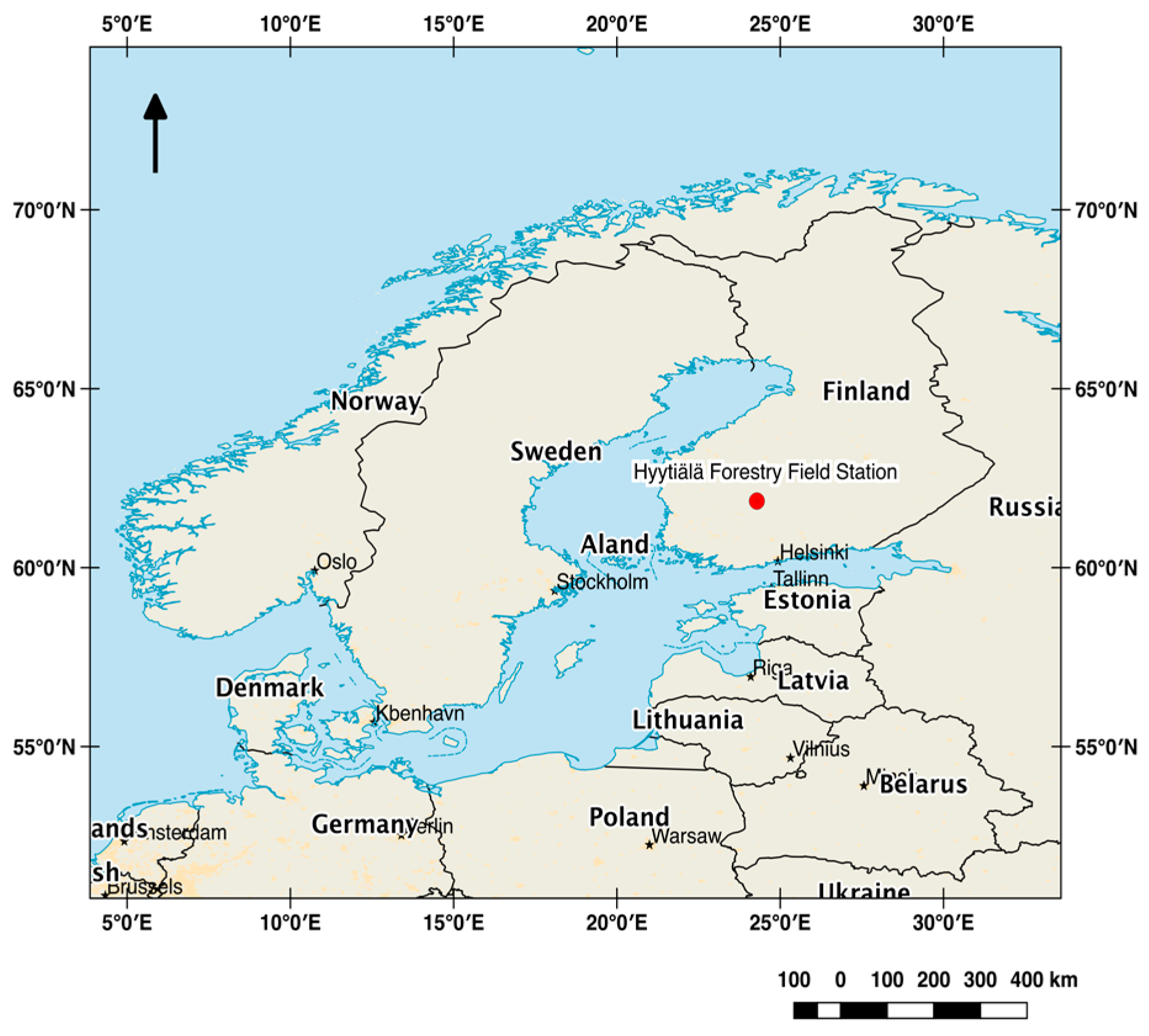
2.1. Study Site
2.2. Data
2.2.1. Flux Tower Data
2.2.2. Satellite Data
2.3. Data Pre-Processing and Computation of VIs
2.4. Time Series Processing
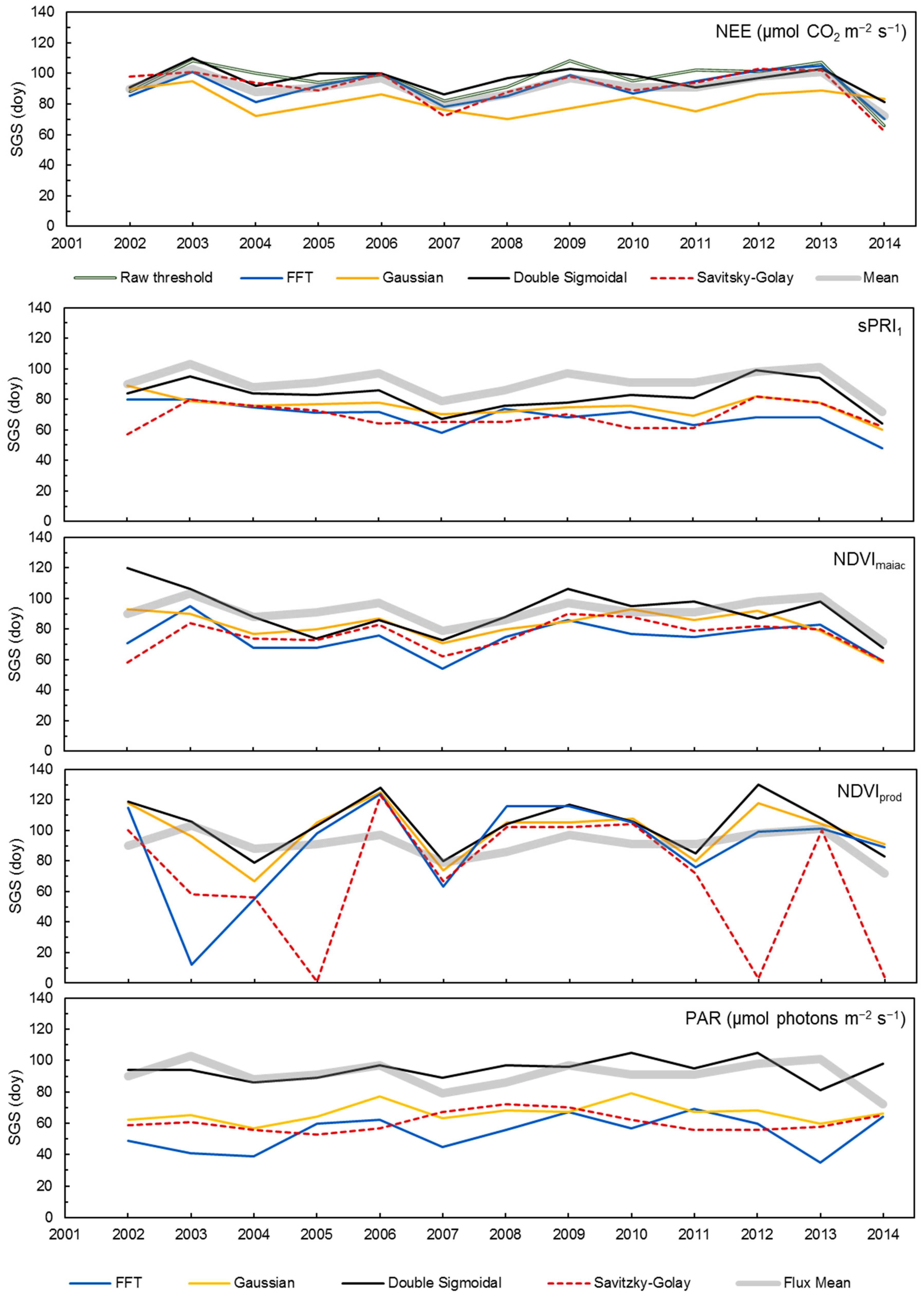
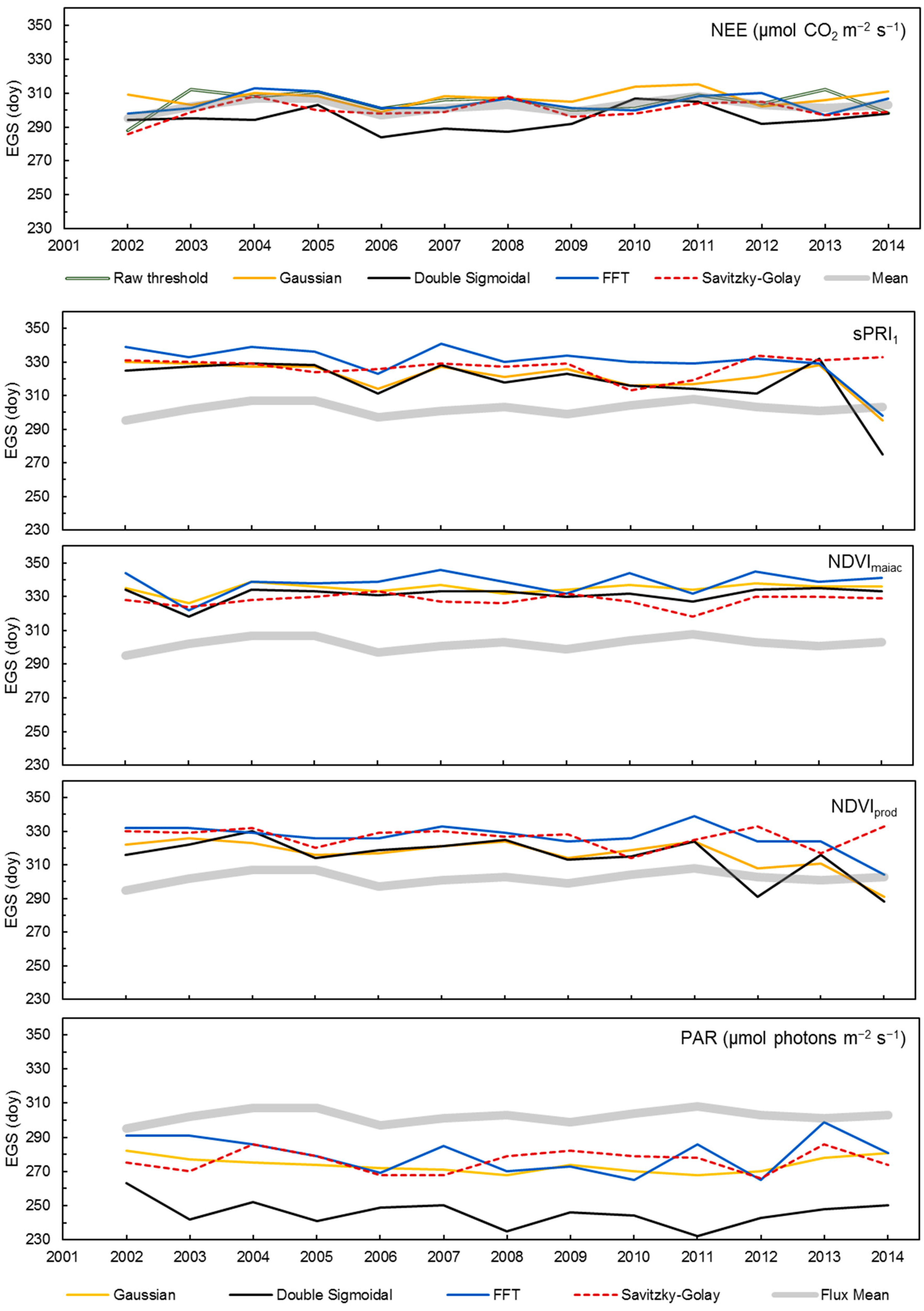
2.5. Extraction of Phenology Metrics
- Determining the metrics based on the smoothed NEE and PAR data [9] implemented in the “Phenex” package. To ensure consistency, a relative threshold set at 20% of NEE/PAR curve amplitude was used to determine SGS and EGS dates.
2.6. Evaluation of Metrics
3. Results
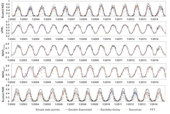
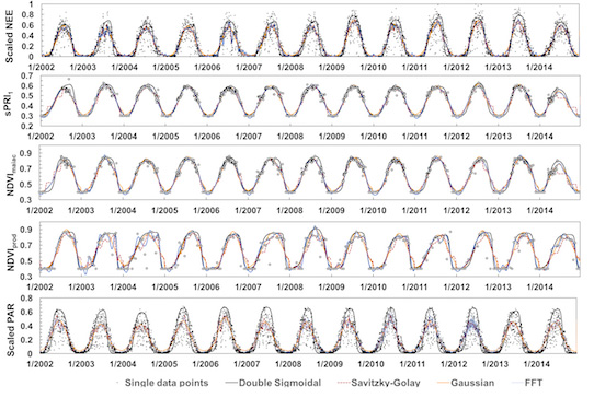
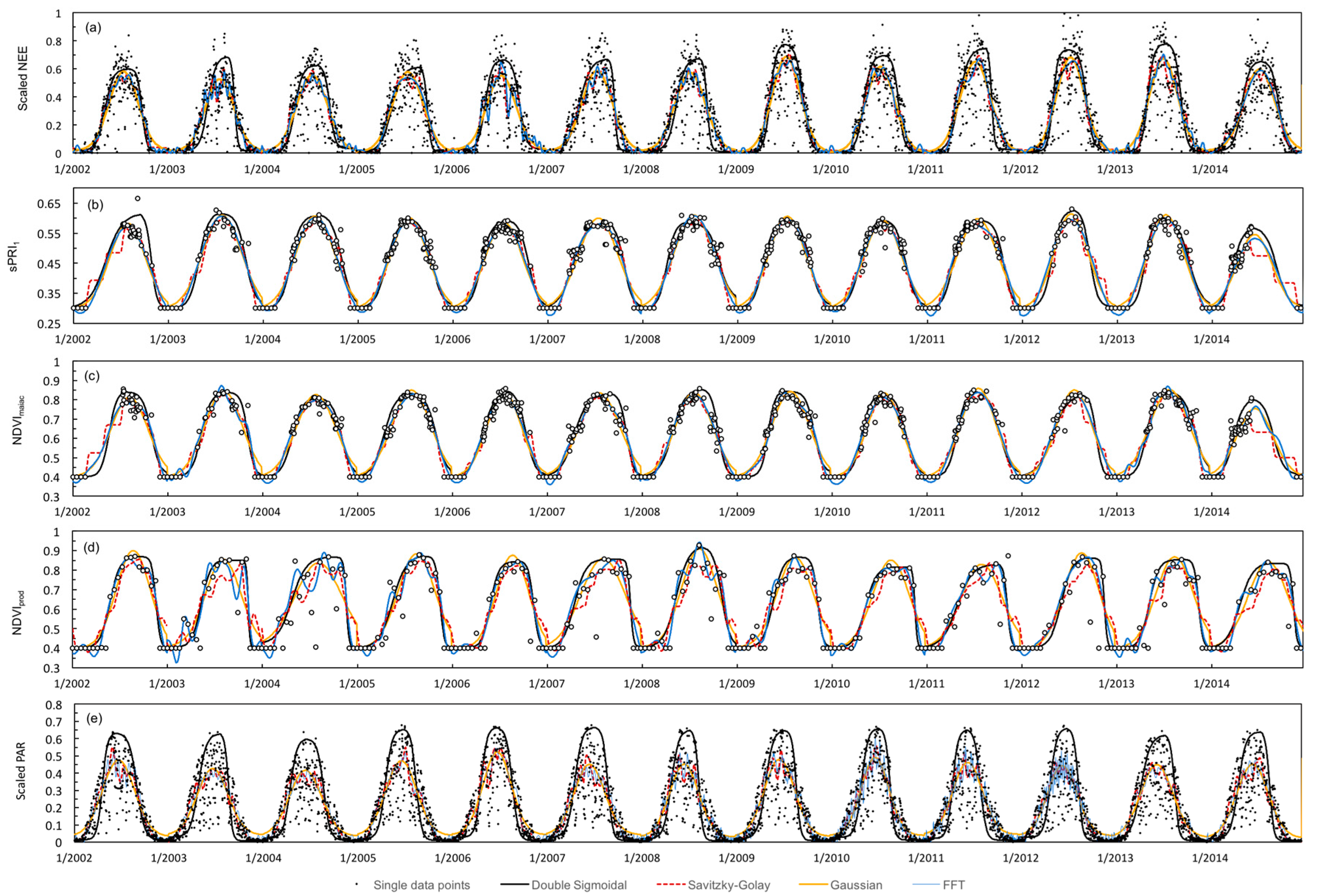
3.1. Time Series Smoothing
3.2. Ground-Derived Metrics
3.3. Satellite-Derived Metrics
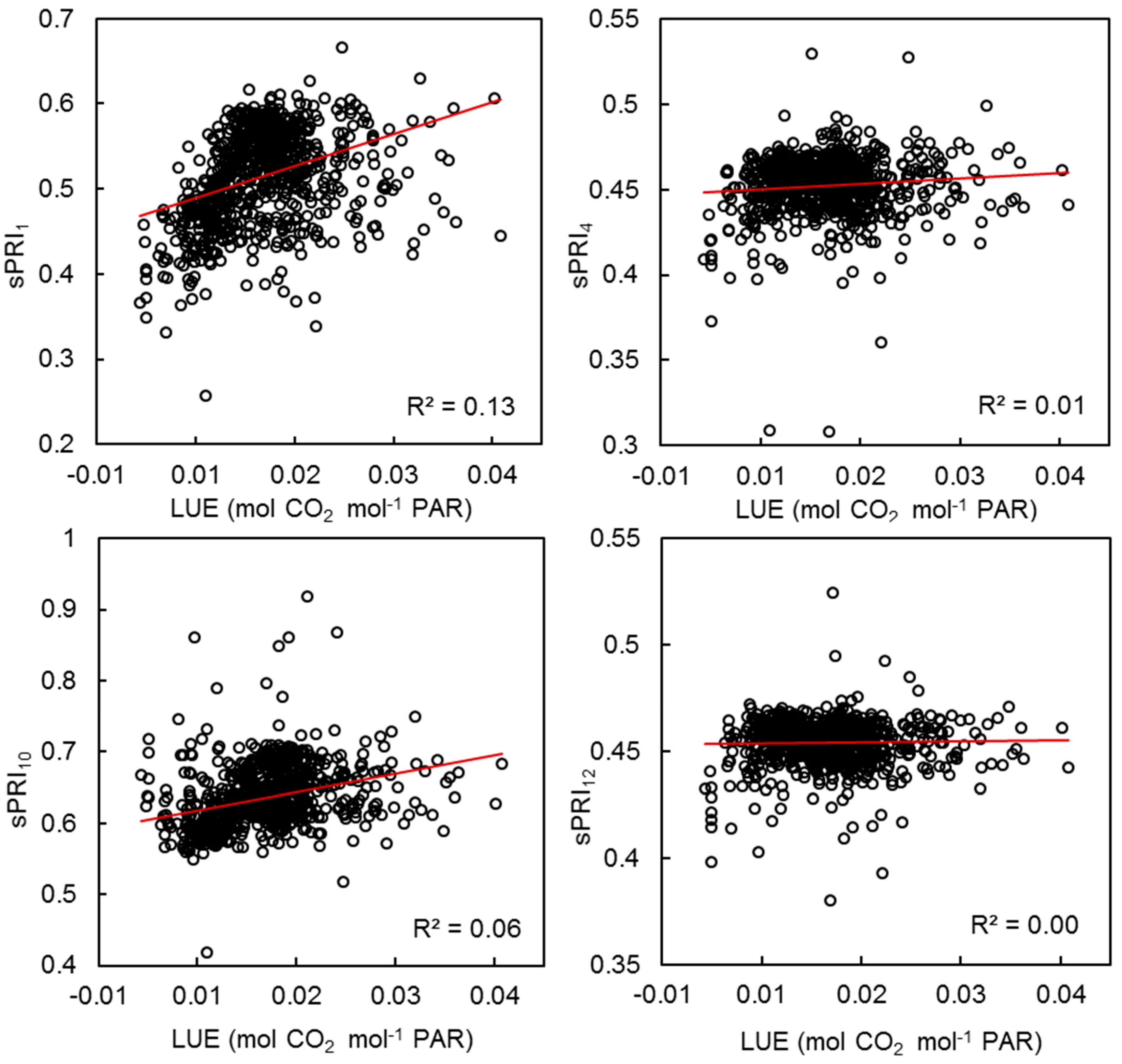
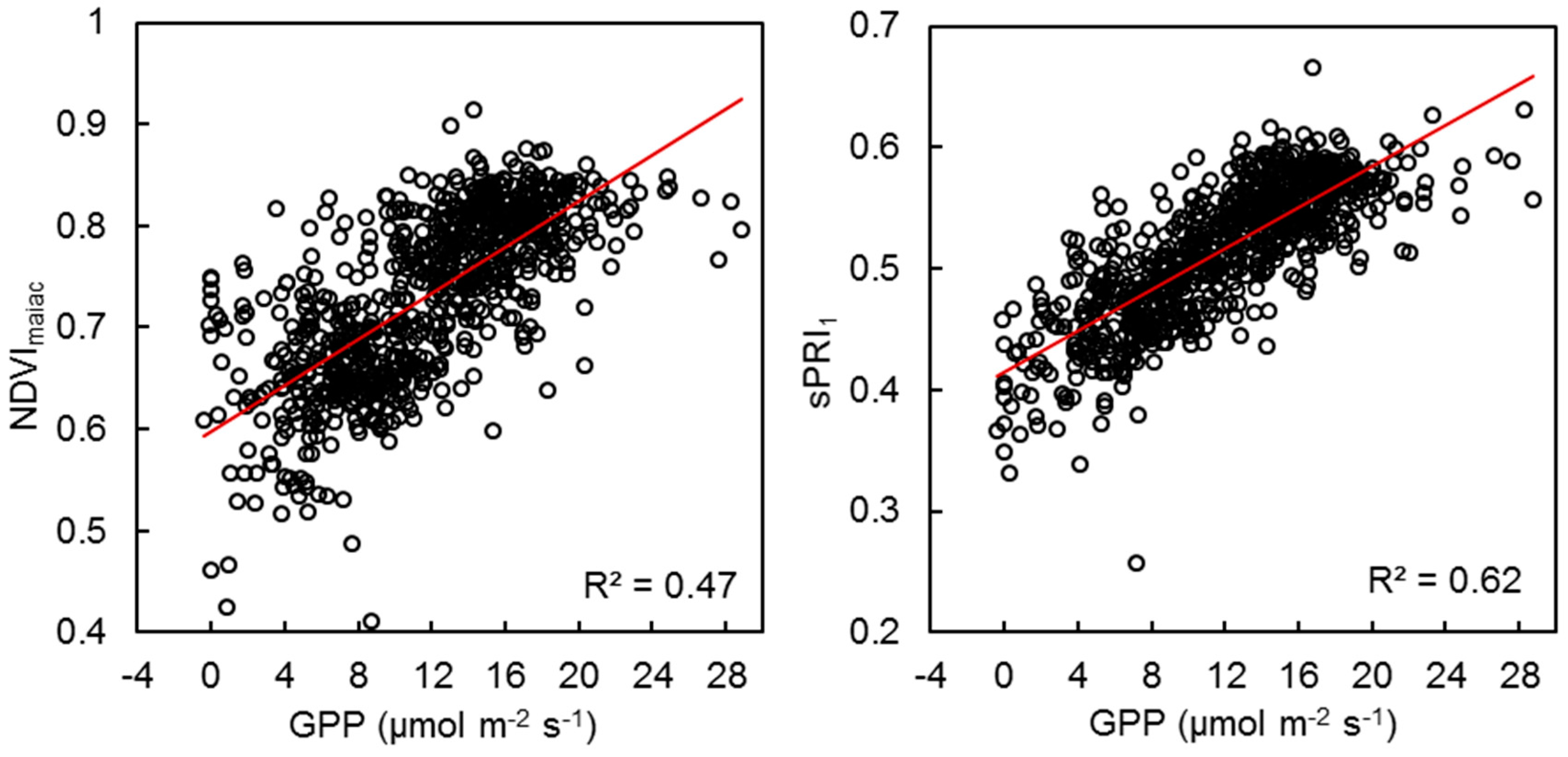
3.4. VI Predictability of Photosynthetic Activity and LUE
3.5. Validation and Inter-Comparison of MODIS-Based Metrics
4. Discussion
4.1. Performances of MAIAC VIs and NDVIprod
4.2. PRI as an Indicator of Photosynthetic Activity and Phenology
4.3. Uncertainties
5. Conclusions
Acknowledgments
Author Contributions
Conflicts of Interest
References
- IPCC. Climate Change 2014: Impacts, Adaptation, and Vulnerability. Part A: Global and Sectoral Aspects. Contribution of Working Group II to the Fifth Assessment Report of the Intergovernmental Panel on Climate Change; Cambridge University Press: Cambridge, UK, 2014. [Google Scholar]
- Baldocchi, D. Assessing the eddy covariance technique for evaluating carbon dioxide exchange rates of ecosystems: Past, present and future. Glob. Chang. Biol. 2003, 9, 479–492. [Google Scholar] [CrossRef]
- Goulden, M.L.; Munger, J.W.; Fan, S.-M.; Daube, B.C.; Wofsy, S.C. Exchange of carbon dioxide by a deciduous forest: Response to interannual climate variability. Science 1996, 271, 1576–1578. [Google Scholar] [CrossRef]
- Reed, B.C.; Brown, J.F.; Vanderzee, D.; Loveland, T.R.; Merchant, J.W.; Ohlen, D.O. Measuring phenological variabilty from satellite imagery. J. Veg. Sci. 1994, 5, 703–714. [Google Scholar] [CrossRef]
- White, M.A.; Hoffman, F.; Hargrove, W.W.; Nemani, R.R. A global framework for monitoring phenological responses to climate change. Geophys. Res. Lett. 2005, 32, L04705. [Google Scholar] [CrossRef]
- De Beurs, K.M.; Henebry, G.M. Land surface phenology and temperature variation in the international geosphere-biosphere program high-latitude transects. Glob. Chang. Biol. 2005, 11, 779–790. [Google Scholar] [CrossRef]
- Wang, C.; Guo, H.; Zhang, L.; Liu, S.; Qiu, Y.; Sun, Z. Assessing phenological change and climatic control of alpine grasslands in the Tibetan plateau with MODIS time series. Int. J. Biometeorol. 2014, 59, 11–23. [Google Scholar] [CrossRef] [PubMed]
- Zhou, L.; Tucker, C.J.; Kaufmann, R.K.; Slayback, D.; Shabanov, N.V.; Myneni, R.B. Variations in northern vegetation activity inferred from satellite data of vegetation index during 1981 to 1999. J. Geophys. Res. Atmos. 2001, 106, 20069–20083. [Google Scholar] [CrossRef]
- Balzarolo, M.; Vicca, S.; Nguy-Robertson, A.L.; Bonal, D.; Elbers, J.A.; Fu, Y.H.; Grünwald, T.; Horemans, J.A.; Papale, D.; Peñuelas, J.; et al. Matching the phenology of net ecosystem exchange and vegetation indices estimated with MODIS and FLUXNET in-situ observations. Remote Sens. Environ. 2016, 174, 290–300. [Google Scholar] [CrossRef]
- Böttcher, K.; Aurela, M.; Kervinen, M.; Markkanen, T.; Mattila, O.-P.; Kolari, P.; Metsämäki, S.; Aalto, T.; Arslan, A.N.; Pulliainen, J. MODIS time-series-derived indicators for the beginning of the growing season in boreal coniferous forest—A comparison with CO2 flux measurements and phenological observations in Finland. Remote Sens. Environ. 2014, 140, 625–638. [Google Scholar] [CrossRef]
- Hmimina, G.; Dufrêne, E.; Pontailler, J.Y.; Delpierre, N.; Aubinet, M.; Caquet, B.; de Grandcourt, A.; Burban, B.; Flechard, C.; Granier, A.; et al. Evaluation of the potential of MODIS satellite data to predict vegetation phenology in different biomes: An investigation using ground-based NDVI measurements. Remote Sens. Environ. 2013, 132, 145–158. [Google Scholar] [CrossRef]
- Tucker, C.J. Red and photographic infrared linear combinations for monitoring vegetation. Remote Sens. Environ. 1979, 8, 127–150. [Google Scholar] [CrossRef]
- Myneni, R.B.; Hoffmann, S.; Knyazikhin, Y.; Privette, J.L.; Glassy, J.; Tian, Y.; Wang, Y.; Song, X.; Zhang, Y.; Smith, G.R.; et al. Global products of vegetation leaf area and fraction absorbed PAR from year one of MODIS data. Remote Sens. Environ. 2002, 83, 214–231. [Google Scholar] [CrossRef]
- Wong, C.Y.; Gamon, J.A. The photochemical reflectance index provides an optical indicator of spring photosynthetic activation in evergreen conifers. New Phytol. 2015, 206, 196–208. [Google Scholar] [CrossRef] [PubMed]
- Garbulsky, M.F.; Peñuelas, J.; Papale, D.; Ardö, J.; Goulden, M.L.; Kiely, G.; Richardson, A.D.; Rotenberg, E.; Veenendaal, E.M.; Filella, I. Patterns and controls of the variability of radiation use efficiency and primary productivity across terrestrial ecosystems. Glob. Ecol. Biogeogr. 2010, 19, 253–267. [Google Scholar] [CrossRef]
- Huemmrich, K.F.; Gamon, J.A.; Tweedie, C.E.; Oberbauer, S.F.; Kinoshita, G.; Houston, S.; Kuchy, A.; Hollister, R.D.; Kwon, H.; Mano, M. Remote sensing of tundra gross ecosystem productivity and light use efficiency under varying temperature and moisture conditions. Remote Sens. Environ. 2010, 114, 481–489. [Google Scholar] [CrossRef]
- Gamon, J.; Penuelas, J.; Field, C. A narrow-waveband spectral index that tracks diurnal changes in photosynthetic efficiency. Remote Sens. Environ. 1992, 41, 35–44. [Google Scholar] [CrossRef]
- Gamon, J.; Serrano, L.; Surfus, J. The photochemical reflectance index: An optical indicator of photosynthetic radiation use efficiency across species, functional types, and nutrient levels. Oecologia 1997, 112, 492–501. [Google Scholar] [CrossRef]
- Porcar-Castell, A.; Garcia-Plazaola, J.; Nichol, C.; Kolari, P.; Olascoaga, B.; Kuusinen, N.; Fernández-Marín, B.; Pulkkinen, M.; Juurola, E.; Nikinmaa, E. Physiology of the seasonal relationship between the photochemical reflectance index and photosynthetic light use efficency. Oecologia 2012, 170, 313–323. [Google Scholar] [CrossRef] [PubMed]
- Gamon, J.; Kovalchuck, O.; Wong, C.; Harris, A.; Garrity, S. Monitoring seasonal and diurnal changes in photosynthetic pigments with automated PRI and NDVI sensors. Biogeosciences 2015, 12, 4149–4159. [Google Scholar] [CrossRef]
- Asner, G.P.; Nepstad, D.; Cardinot, G.; Ray, D. Drought stress and carbon uptake in an Amazon forest measured with spaceborne imaging spectroscopy. Proc. Natl. Acad. Sci. USA 2004, 101, 6039–6044. [Google Scholar] [CrossRef] [PubMed]
- Hilker, T.; Coops, N.C.; Hall, F.G.; Nichol, C.J.; Lyapustin, A.; Black, T.A.; Wulder, M.A.; Leuning, R.; Barr, A.; Hollinger, D.Y.; et al. Inferring terrestrial photosynthetic light use efficiency of temperate ecosystems from space. J. Geophys. Res. 2011, 116. [Google Scholar] [CrossRef]
- Nichol, C.; Huemmrich, K.; Black, T.; Jarvis, P.; Walthall, C.; Grace, J.; Hall, F. Remote sensing of photosynthetic-light-use efficiency of boreal forest. Agric. For. Meteorol. 2000, 101, 131–142. [Google Scholar] [CrossRef]
- Nichol, C.; Lloyd, J.; Shibistova, O.; Arneth, A.; Roser, C.; Knohl, A.; Matsubara, S.; Grace, J. Remote sensing of photosynthetic-light-use efficiency of a Siberian boreal forest. Tellus B Chem. Phys. Meteorol. 2002, 54, 667–687. [Google Scholar] [CrossRef]
- Middleton, E.; Cheng, Y.; Hilker, T.; Huemmrich, K.; Black, T.; Krishnan, P.; Coops, N. Linking foliage spectral responses to canopy-level ecosystem photosynthetic light-use efficiency at a Douglas-fir forest in Canada. Can. J. Remote Sens. 2009, 35, 166–188. [Google Scholar] [CrossRef]
- Drolet, G.G.; Huemmrich, K.F.; Hall, F.G.; Middleton, E.M.; Black, T.A.; Barr, A.G.; Margolis, H.A. A MODIS-derived photochemical reflectance index to detect inter-annual variations in the photosynthetic light-use efficiency of a boreal deciduous forest. Remote Sens. Environ. 2005, 98, 212–224. [Google Scholar] [CrossRef]
- Drolet, G.G.; Middleton, E.M.; Huemmrich, K.F.; Hall, F.G.; Amiro, B.D.; Barr, A.G.; Black, T.A.; McCaughey, J.H.; Margolis, H.A. Regional mapping of gross light-use efficiency using MODIS spectral indices. Remote Sens. Environ. 2008, 112, 3064–3078. [Google Scholar] [CrossRef]
- Garbulsky, M.F.; Peñuelas, J.; Papale, D.; Filella, I. Remote estimation of carbon dioxide uptake by a mediterranean forest. Glob. Chang. Biol. 2008, 14, 2860–2867. [Google Scholar] [CrossRef]
- Goerner, A.; Reichstein, M.; Rambal, S. Tracking seasonal drought effects on ecosystem light use efficiency with satellite-based PRI in a mediterranean forest. Remote Sens. Environ. 2009, 113, 1101–1111. [Google Scholar] [CrossRef]
- Goerner, A.; Reichstein, M.; Tomelleri, E.; Hanan, N.; Rambal, S.; Papale, D.; Dragoni, D.; Schmullius, C. Remote sensing of ecosystem light use efficiency with MODIS-based PRI. Biogeosciences 2011, 8, 189–202. [Google Scholar] [CrossRef]
- Guarini, R.; Nichol, C.; Clement, R.; Loizzo, R.; Grace, J.; Borghetti, M. The utility of MODIS-sPRI for investigating the photosynthetic light-use efficiency in a mediterranean deciduous forest. Int. J. Remote Sens. 2014, 35, 6157–6172. [Google Scholar] [CrossRef]
- Rahman, A.F.; Cordova, V.D.; Gamon, J.A.; Schmid, H.P.; Sims, D.A. Potential of MODIS ocean bands for estimating CO2 flux from terrestrial vegetation: A novel approach. Geophys. Res. Lett. 2004, 31, L10503. [Google Scholar] [CrossRef]
- Garbulsky, M.F.; Peñuelas, J.; Gamon, J.; Inoue, Y.; Filella, I. The photochemical reflectance index (PRI) and the remote sensing of leaf, canopy and ecosystem radiation use efficiencies: A review and meta-analysis. Remote Sens. Environ. 2011, 115, 281–297. [Google Scholar] [CrossRef]
- Grace, J.; Nichol, C.; Disney, M.; Lewis, P.; Quaife, T.; Bowyer, P. Can we measure terrestrial photosynthesis from space directly, using spectral reflectance and fluorescence? Glob. Chang. Biol. 2007, 13, 1484–1497. [Google Scholar] [CrossRef]
- Huete, A.R.; Didan, K.; Miura, T.; Rodriguez, E.P.; Gao, X.; Ferreira, L.G. Overview of the radiometric and biophysical performance of the MODIS indices. Remote Sens. Environ. 2002, 83, 195–213. [Google Scholar] [CrossRef]
- Jönsson, P.; Ekhlund, L. Seasonality extraction by function-fitting to time series of satellite data. IEEE Trans. Geosci. Remote Sens. 2002, 40, 1824–1832. [Google Scholar] [CrossRef]
- Atkinson, P.M.; Jeganathan, C.; Dash, J.; Atzberger, C. Inter-comparison of four models for smoothing satellite sensor time-series data to estimate vegetation phenology. Remote Sens. Environ. 2012, 123, 400–417. [Google Scholar] [CrossRef]
- Beck, P.S.A.; Atzberger, C.; Høgda, K.A.; Johansen, B.; Skidmore, A.K. Improved monitoring of vegetation dynamics at very high latitudes: A new method using MODIS NDVI. Remote Sens. Environ. 2006, 100, 321–334. [Google Scholar] [CrossRef]
- Middleton, E.; Huemmrich, K.F.; Landis, D.; Black, T.A.; Barr, A.G.; McCaughey, J.H.; Hall, F. Remote sensing of ecosystem light use efficiency using MODIS. Remote Sens. Environ. 2016, 187, 345–366. [Google Scholar] [CrossRef]
- Lyapustin, A.; Wang, Y.; Laszlo, I.; Kahn, R.; Korkin, S.; Remer, L.; Levy, R.; Reid, J.S. Multiangle implementation of atmospheric correction (MAIAC): 2. Aerosol algorithm. J. Geophys. Res. 2011, 116. [Google Scholar] [CrossRef]
- Lyapustin, A.I.; Wang, Y.; Laszlo, I.; Hilker, T.; G.Hall, F.; Sellers, P.J.; Tucker, C.J.; Korkin, S.V. Multi-angle implementation of atmospheric correction for modis (MAIAC): 3. Atmospheric correction. Remote Sens. Environ. 2012, 127, 385–393. [Google Scholar] [CrossRef]
- Hilker, T.; Lyapustin, A.; Hall, F.G.; Wang, Y.; Coops, N.C.; Drolet, G.; Black, T.A. An assessment of photosynthetic light use efficiency from space: Modeling the atmospheric and directional impacts on PRI reflectance. Remote Sens. Environ. 2009, 113, 2463–2475. [Google Scholar] [CrossRef]
- Suni, T.; Rinne, J.; Reissell, A.; Altimir, N. Long-term measurements of surface fluxes above a Scots pine forest in Hyytiala, southern Finland, 1996–2001. Boreal Environ. Res. 2003, 8, 287–301. [Google Scholar]
- Wang, Q.; Tenhunen, J.; Dinh, N.Q.; Reichstein, M.; Vesala, T.; Keronen, P. Similarities in ground- and satellite-based NDVI time series and their relationship to physiological activity of a scots pine forest in Finland. Remote Sens. Environ. 2004, 93, 225–237. [Google Scholar] [CrossRef]
- Aubinet, M.; Vesala, T.; Papale, D. Eddy Covariance: A Practical Guide to Measurement and Data Analysis; Springer Science & Business Media: Dordrecht, The Netherlands, 2012. [Google Scholar]
- Mammarella, I.; Peltola, O.; Nordbo, A.; Järvi, L.; Rannik, Ü. Quantifying the uncertainty of eddy covariance fluxes due to the use of different software packages and combinations of processing steps in two contrasting ecosystems. Atmos. Meas. Tech. 2016, 9, 4915–4933. [Google Scholar] [CrossRef]
- Mammarella, I.; Launiainen, S.; Gronholm, T.; Keronen, P.; Pumpanen, J.; Rannik, Ü.; Vesala, T. Relative humidity effect on the high frequency attenuation of water vapour flux measured by a closed-path eddy covariance system. J. Atmos. Ocean. Technol. 2009, 26, 1856–1866. [Google Scholar] [CrossRef]
- Kolari, P.; Kulmala, L.; Pumpanen, J.; Launiainen, S.; Ilvesniemi, H.; Hari, P.; Nikinmaa, E. CO2 exchange and component CO2 fluxes of a boreal Scots pine forest. Boreal Environ. Res. 2009, 14, 761–783. [Google Scholar]
- Monteith, J. Climate and the efficiency of crop production in Britain. Philos. Trans. R. Soc. Lond. Biol. 1977, 281, 277–294. [Google Scholar] [CrossRef]
- Hird, J.N.; McDermid, G.J. Noise reduction of NDVI time series: An empirical comparison of selected techniques. Remote Sens. Environ. 2009, 113, 248–258. [Google Scholar] [CrossRef]
- Eklundh, L.; Jönsson, P. Remote Sensing Time Series. TIMESAT: A Software Package for Time-Series Processing and Assessment of Vegetation Dynamics; Springer: Cham, Switzerland, 2015; pp. 141–158. [Google Scholar]
- Doktor, D.; Lange, M. Phenex Version 1.0.3—Auxiliary Functions for Phenological Data Analysis. A Package for R-Statistical Software. Available online: https://cran.r-project.org/web/packages/phenex/phenex.pdf (accessed on 28 April 2016).
- Viovy, N.; Arino, O.; Belward, A.S. The Best Index Slope Extraction (BISE): A method for reducing noise in NDVI time-series. Int. J. Remote Sens. 1992, 13, 1585–1590. [Google Scholar] [CrossRef]
- Tan, B.; Morisette, J.T.; Wolfe, R.E.; Gao, F.; Ederer, G.A.; Nightingale, J.; Pedelty, J.A. An enhanced TIMESAT algorithm for estimating vegetation phenology metrics from MODIS data. IEEE J. Sel. Top. Appl. Earth Obs. Remote Sens. 2011, 4, 361–371. [Google Scholar] [CrossRef]
- Zhang, X.; Friedl, M.; Schaaf, C.; Strahler, A.; Hodges, J.; Gao, F.; Reed, B.; Huete, A. Monitoring vegetation phenology using MODIS. Remote Sens. Environ. 2003, 84, 471–475. [Google Scholar] [CrossRef]
- Soudani, K.; le Maire, G.; Dufrêne, E.; François, C.; Delpierre, N.; Ulrich, E.; Cecchini, S. Evaluation of the onset of green-up in temperate deciduous broadleaf forests derived from moderate resolution imaging spectroradiometer (MODIS) data. Remote Sens. Environ. 2008, 112, 2643–2655. [Google Scholar] [CrossRef]
- Garrity, S.R.; Bohrer, G.; Maurer, K.D.; Mueller, K.L.; Vogel, C.S.; Curtis, P.S. A comparison of multiple phenology data sources for estimating seasonal transitions in deciduous forest carbon exchange. Agric. For. Meteorol. 2011, 151, 1741–1752. [Google Scholar] [CrossRef]
- Sellers, P.J.; Tucker, C.J.; Collatz, G.J.; Los, S.O.; Justice, C.O.; Dazlich, D.A.; Randall, D.A. A global 1° by 1° NDVI data set for climate studies. Part 2: The generation of global fields of terrestrial biophysical parameters from the NDVI. Int. J. Remote Sens. 2007, 15, 3519–3545. [Google Scholar] [CrossRef]
- Chen, J.; Jönsson, P.; Tamura, M.; Gu, Z.; Matsushita, B.; Eklundh, L. A simple method for reconstructing a high-quality NDVI time-series data set based on the Savitzky–Golay filter. Remote Sens. Environ. 2004, 91, 332–344. [Google Scholar] [CrossRef]
- Tanja, S.; Berninger, F.; Vesala, T.; Markkanen, T.; Hari, P.; Mäkelä, A.; Ilvesniemi, H.; Hänninen, H.; Nikinmaa, E.; Huttula, T.; et al. Air temperature triggers the recovery of evergreen boreal forest photosynthesis in spring. Glob. Chang. Biol. 2003, 9, 1410–1426. [Google Scholar] [CrossRef]
- Thum, T.; Aalto, T.; Laurila, T.; Aurela, M.; Hatakka, J.; Lindroth, A.; Vesala, T. Spring initiation and autumn cessation of boreal coniferous forest CO2 exchange assessed by meteorological and biological variables. Tellus B 2009, 61, 701–717. [Google Scholar] [CrossRef]
- Liu, Y.; Wu, C.; Peng, D.; Xu, S.; Gonsamo, A.; Jassal, R.S.; Altaf Arain, M.; Lu, L.; Fang, B.; Chen, J.M. Improved modeling of land surface phenology using MODIS land surface reflectance and temperature at evergreen needleleaf forests of central North America. Remote Sens. Environ. 2016, 176, 152–162. [Google Scholar] [CrossRef]
- Lyapustin, A.; Wang, Y.; Frey, R. An automatic cloud mask algorithm based on time series of MODIS measurements. J. Geophys. Res. 2008, 113, D16207. [Google Scholar] [CrossRef]
- Richardson, A.D.; Keenan, T.F.; Migliavacca, M.; Ryu, Y.; Sonnentag, O.; Toomey, M. Climate change, phenology, and phenological control of vegetation feedbacks to the climate system. Agric. For. Meteorol. 2013, 169, 156–173. [Google Scholar] [CrossRef]
- Gitelsen, A.; Gamon, J. The need for a common basis for defining light use efficiency: Implications for productivity estimation. Pap. Nat. Resour. 2015, 483, 196–201. [Google Scholar] [CrossRef]
- Nakaji, T.; Ide, R.; Kosugi, K.; Ohkubo, S.; Nasahara, K.M.; Saigusa, N.; Oguma, H. Utility of spectral vegetation indices for estimation of light use efficiency in coniferous forests in Japan. Agric. For. Meteorol. 2008, 148, 776–787. [Google Scholar] [CrossRef]
- Nakaji, T.; Kosugi, Y.; Takanashi, S.; Niiyama, K.; Noguchi, S.; Tani, M.; Oguma, H.; Nik, A.R.; Kassim, A.R. Estimation of light use efficiency through a combinational use of the photochemical reflectance index and vapour pressure deficit in an evergreen tropical rainforest at Pasoh, Peninsular Malaysia. Remote Sens. Environ. 2014, 150, 82–92. [Google Scholar] [CrossRef]
- Nagai, S.; Saitoh, T.M.; Kobayashi, H.; Ishihara, M.; Suzuki, R.; Motokha, T.; Nasahara, K.N.; Muraoka, H. In situ examination of the relationship between various vegetation indices and canopy phenology in an evergreen coniferous forest, Japan. Int. J. Remote Sens. 2012, 19, 6202–6214. [Google Scholar] [CrossRef]
- Kolari, P.; Lappalainen, H.; Hänninen, H.; Hari, P. Relationship between temperature and the seasonal course of photosynthesis in Scots pine at northern timberline and in southern boreal zone. Tellus B 2007, 59, 542–552. [Google Scholar] [CrossRef]
- Delbart, N.; Le Toan, T.; Kergoat, L.; Fedotova, V. Remote sensing of spring phenology in boreal regions: A free of snow-effect method using NOAA-AVHRR and SPOT-VGT data (1982–2004). Remote Sens. Environ. 2006, 101, 52–62. [Google Scholar] [CrossRef]


| Smoothing Technique | Description | Implemented in (Modified Versions) |
|---|---|---|
| Gaussian function | Applies symmetrical or asymmetrical Gaussian function that has the best fit to a series of data points (C implementation). | Ekhlund and Jönsson [36] Tan et al. [54] |
| Double sigmoidal function | Applies a double sigmoidal function to data values that has the best fit to a series of data points (C implementation). | Zhang et al. [55] Soudani et al. [56] Garrity et al. [57] Hmimina et al. [11] Wong and Gamon [14] |
| Fast Fourier transform | Fast Fourier transform algorithm (smoothing intensity parameter default value = 3) which decomposes noise-affected time series into simpler periodic signals using sine and cosine functions. | Sellers et al. [58] Wang et al. [44] |
| Savitzky–Golay filter | Smooths data values with a Savitzky–Golay filter, which is based on local least squares polynomial approximation (default window size setting = 7, degree of fitting polynomial = 2 and smoothing repetition = 10). | Chen et al. [59] Ekhlund and Jönsson [51] Balzarolo et al. [9] Böttcher et al. [10] |
| VI | NDVImaiac | sPRI1 | sPRI4 | sPRI10 | sPRI12 | |||||
|---|---|---|---|---|---|---|---|---|---|---|
| Parameter | LUE | GPP | LUE | GPP | LUE | GPP | LUE | GPP | LUE | GPP |
| R2 | 0.16 | 0.47 | 0.13 | 0.63 | 0.01 | 0.14 | 0.06 | 0.02 | 0.00 | 0.11 |
| r | 0.51 | 0.73 | 0.39 | 0.80 | 0.04 | 0.34 | 0.40 | 0.22 | −0.07 | 0.25 |
| p-value | <0.05 | <0.05 | <0.05 | <0.05 | 0.24 | <0.05 | <0.05 | <0.05 | 0.06 | <0.05 |
| Vegetation Index | Method | r | R2 | RMSE (Days) | Bias (Days) |
|---|---|---|---|---|---|
| sPRI1 * | Gaussian | 0.83 | 0.74 | 17.5 | −16.8 |
| Double Sigmoidal | 0.84 | 0.80 | 9.8 | −8.7 | |
| FFT | 0.33 | 0.53 | 23.9 | −23.1 | |
| Savitzky–Golay | 0.57 | 0.36 | 22.6 | −21.4 | |
| NDVImaiac * | Gaussian | 0.63 | 0.66 | 11.2 | −9.7 |
| Double Sigmoidal | 0.64 | 0.60 | 7.9 | −2.3 | |
| FFT | 0.90 | 0.79 | 17.2 | −16.5 | |
| Savitzky–Golay | 0.77 | 0.73 | 14.8 | −14.0 | |
| NDVIprod ** | Gaussian | 0.37 | 0.21 | 17.3 | 12.6 |
| Double Sigmoidal | 0.66 | 0.44 | 18.0 | 8.6 | |
| FFT | 0.10 | 0.00 | 31.6 | −1.2 | |
| Savitzky–Golay | 0.11 | 0.09 | 45.2 | −22.5 | |
| PAR ** | Gaussian | 0.15 | 0.01 | 26.5 | −24.7 |
| Double Sigmoidal | −0.04 | 0.00 | 11.3 | 3.23 | |
| FFT | −0.08 | 0.04 | 39.8 | −36.9 | |
| Savitzky–Golay | −0.32 | 0.13 | 32.3 | −30.15 |
| Vegetation Index | Method | r | R2 | RMSE | Bias |
|---|---|---|---|---|---|
| sPRI1 * | Gaussian | 0.26 | 0.03 | 17.6 | 14.9 |
| Double Sigmoidal | 0.25 | 0.03 | 17.6 | 16.5 | |
| FFT | 0.18 | 0.05 | 26.9 | 26.4 | |
| Savitzky–Golay | −0.26 | 0.06 | 25.1 | 23.9 | |
| NDVImaiac * | Gaussian | −0.27 | 0.02 | 22.5 | 21.3 |
| Double Sigmoidal | 0.01 | 0.00 | 21.2 | 19.6 | |
| FFT | −0.07 | 0.00 | 31.3 | 30.7 | |
| Savitzky–Golay | −0.49 | 0.18 | 25.8 | 24.6 | |
| NDVIprod ** | Gaussian | 0.33 | 0.05 | 32.8 | 29.0 |
| Double Sigmoidal | −0.08 | 0.01 | 29.6 | 32.5 | |
| FFT | −0.19 | 0.02 | 37.0 | 36.2 | |
| Savitzky–Golay | −0.42 | 0.25 | 26.3 | 25.5 | |
| PAR ** | Gaussian | −0.43 | 0.17 | 29.3 | −28.5 |
| Double Sigmoidal | −0.51 | 0.41 | 57.5 | −56.5 | |
| FFT | −0.13 | 0.00 | 25.0 | −22.3 | |
| Savitzky–Golay | 0.26 | 0.11 | 26.9 | −26.2 |
© 2017 by the authors; licensee MDPI, Basel, Switzerland. This article is an open access article distributed under the terms and conditions of the Creative Commons Attribution (CC-BY) license (http://creativecommons.org/licenses/by/4.0/).
Share and Cite
Ulsig, L.; Nichol, C.J.; Huemmrich, K.F.; Landis, D.R.; Middleton, E.M.; Lyapustin, A.I.; Mammarella, I.; Levula, J.; Porcar-Castell, A. Detecting Inter-Annual Variations in the Phenology of Evergreen Conifers Using Long-Term MODIS Vegetation Index Time Series. Remote Sens. 2017, 9, 49. https://doi.org/10.3390/rs9010049
Ulsig L, Nichol CJ, Huemmrich KF, Landis DR, Middleton EM, Lyapustin AI, Mammarella I, Levula J, Porcar-Castell A. Detecting Inter-Annual Variations in the Phenology of Evergreen Conifers Using Long-Term MODIS Vegetation Index Time Series. Remote Sensing. 2017; 9(1):49. https://doi.org/10.3390/rs9010049
Chicago/Turabian StyleUlsig, Laura, Caroline J. Nichol, Karl F. Huemmrich, David R. Landis, Elizabeth M. Middleton, Alexei I. Lyapustin, Ivan Mammarella, Janne Levula, and Albert Porcar-Castell. 2017. "Detecting Inter-Annual Variations in the Phenology of Evergreen Conifers Using Long-Term MODIS Vegetation Index Time Series" Remote Sensing 9, no. 1: 49. https://doi.org/10.3390/rs9010049