Image Fusion for Spatial Enhancement of Hyperspectral Image via Pixel Group Based Non-Local Sparse Representation

Abstract

Restricted by technical and budget constraints, hyperspectral images (HSIs) are usually obtained with low spatial resolution. In order to improve the spatial resolution of a given hyperspectral image, a new spatial and spectral image fusion approach via pixel group based non-local sparse representation is proposed, which exploits the spectral sparsity and spectral non-local self-similarity of the hyperspectral image. The proposed approach fuses the hyperspectral image with a high-spatial-resolution multispectral image of the same scene to obtain a hyperspectral image with high spatial and spectral resolutions. The input hyperspectral image is used to train the spectral dictionary, while the sparse codes of the desired HSI are estimated by jointly encoding the similar pixels in each pixel group extracted from the high-spatial-resolution multispectral image. To improve the accuracy of the pixel group based non-local sparse representation, the similar pixels in a pixel group are selected by utilizing both the spectral and spatial information. The performance of the proposed approach is tested on two remote sensing image datasets. Experimental results suggest that the proposed method outperforms a number of sparse representation based fusion techniques, and can preserve the spectral information while recovering the spatial details under large magnification factors.

1. Introduction

Hyperspectral images (HSIs) usually contain dozens or even hundreds of spectral bands. They are useful for accurate terrain detection, military surveillance and medical diagnosis [1]. However, owing to the technical and budget constraints, there is a tradeoff between spectral resolution and spatial resolution, which often implies low spatial resolution of HSIs. This fact may severely impede the practical use of HSIs and, therefore, various spatial resolution enhancement algorithms [2,3,4,5] have been proposed with spatial and spectral fusion approaches playing an important role. In contrast to hyperspectral sensors, multispectral sensors produce images with relatively higher spatial resolution but less spectral bands. Thus, the fusion of these two types of image data supports the integration of the spatial details of a high spatial resolution multispectral image (MSI) and the spectral information of a HSI, thereby producing a HSI with both high spatial and high spectral resolutions.

Multiple spatial and spectral fusion approaches have been developed for the spatial resolution enhancement. Traditionally, hyperspectral images or multispectral images are fused with a high spatial resolution panchromatic (PAN) image, which is commonly called pan-sharpening [5,6,7,8]. Representative algorithms of pan-sharpening include the component substitution based methods [6,7] and the multi-resolution based methods [8]. Component substitution based methods transform the multispectral or hyperspectral image into a certain domain, in which the first component is replaced by the PAN image. In multi-resolution based approaches, the wavelet transform is commonly used to decompose the source images into high and low frequency components. After that, the high frequency component extracted from the PAN image is merged into the multispectral or hyperspectral data. These approaches successfully improve the spatial resolution of the multispectral or hyperspectral image, but they may cause unavoidable spectral or spatial distortion.

Another category of methods implementing spatial–spectral image fusion is unmixing based approaches [9,10,11,12,13]. In such schemes, low spatial resolution hyperspectral data are unmixed into the endmember spectra and the corresponding abundances, and then the abundance maps are fused with the high spatial resolution image of the same scene (such as Red-Green-Blue image or MSI). Based on the fact that neighboring pixels normally share fractions of the same underlying material, Bieniarz et al. [13] employed a jointly sparse model to perform the unmixing of these neighboring pixels. In order to enhance unmixing accuracy, a dictionary trained with MSIs or PAN images from unrelated scenes is used in [12]. However, the performance of these approaches degrades seriously in highly mixed situations [14]. More recently, matrix factorization [4,15] has emerged as a powerful tool in unmixing based approaches, which aims to factorize the image data into two matrices based on a linear spectral mixture model [16]. A coupled nonnegative matrix factorization unmixing approach [4] is proposed where HSI and MSI are separately unmixed. By combining the endmember matrix of the HSI and the abundance matrix of the MSI, the fusion result is generated.

The sparsity property of an image is an effective representation of the image prior knowledge for various kinds of spatial–spectral image fusion tasks [17,18,19,20,21]. In recent years, motivated by the observation that there are only a few materials contributing to each pixel in HSIs [16], sparsity has been introduced in to matrix factorization based algorithms. These approaches do not require prior knowledge of the spatial transform matrix but instead assume that the HSI and the high spatial resolution image have the same sparse coefficients in the spectral domain. The general framework of these approaches [14,22,23,24] can be outlined as follows. Firstly, a spectral dictionary is trained by extracting distinct spectral vectors in the low spatial resolution HSI. Next, the high spatial resolution image is sparsely encoded with the corresponding spectral dictionary, named sparse representation. Finally, the coefficients generated in the sparse representation procedure are used to produce the desired high spatial resolution HSI. Such schemes can always obtain better visual results and lead to the state-of-the-art performance of the challenging spatial resolution enhancement problem.

In this work, a new spatial and spectral fusion algorithm is proposed using the pixel group based non-local sparse representation technique, which exploits the non-local self-similarity of spectral vectors in the HSI. Firstly, a spectral dictionary is trained by the low spatial resolution HSI. Secondly, each pixel of the high spatial resolution MSI is jointly encoded with its similar pixels. Finally, the iterative back-projection technique is employed to refine the resulting image. The contributions of this work can be outlined as follows: (1) Differing from the conventional approaches that employ non-local self-similarity in the spatial domain, this work introduces the non-local self-similarity of the spectral vectors in HSIs to the fusion based spatial resolution enhancement problem. (2) The selection of similar pixels is carried out by utilizing not only the spectral information, but also the spatial information. (3) Rather than processing the fusion procedure pixel by pixel as some previous works reported, a pixel group based scheme is utilized in this work.

The rest of this paper is organized as follows. Section 2 reviews the framework of sparse representation and the spectral dictionary learning technique, and recalls the non-local self-similarity of HSIs. The proposed spatial and spectral fusion method is introduced in detail in Section 3. In Section 4, experimental results and discussions are given to verify the effectiveness of the proposed algorithm. Finally, Section 5 presents the conclusions of this paper.

2. Related Works

Relevant works are introduced in this section, including basic concepts of sparse representation, spectral dictionary learning, and the non-local self-similarity of HSIs.

2.1. Sparse Representation

Sparse representation has proven to be an extremely powerful tool for acquiring, representing, and compressing high-dimensional signals [25]. Given a signal vector $y\in R^L$, sparse representation aims to represent it as the linear combination of certain basis vectors extracted from a basis matrix $D\in R^{L\times k}$ (also called a dictionary) and to seek the sparsest coefficient $\alpha \in R^k$. This process can be expressed as the following optimization problem:

$$\underset{\alpha }{\mathrm{arg\; min}}||\alpha |{|}_{0}s.t.||y-D\alpha |{|}_2\le \epsilon$$

(1)

where $\epsilon \ge 0$ is a preset small constant, which denotes the decomposition error. The notation $||\cdot |{|}_0$ is the L₀-norm counting the number of non-zero elements in the vector.

The above optimization formulated in Equation (1) is a non-deterministic polynomial-time hard (NP-hard) problem, which is very complex to solve. There are two categories of algorithms that have been developed to approximate the optimal solution of this problem. One strategy is to adapt a greedy pursuit algorithm, which selects one or more appropriate basis in the dictionary at each step to iteratively represent the vector to be decomposed. The representative algorithms include the orthogonal matching pursuit (OMP) [26] and many improved versions of OMP [27].

Another strategy is to use a convex optimization algorithm, which replaces the L₀-norm with the L₁-norm in Equation (1), represented by methods such as Basic Pursuit (BP) [28], Lasso [29] and the iterative thresholding algorithm [30].

2.2. Spectral Dictionary Learning

Research results have shown that a HSI can be sparsely represented in the spectral domain [16]. Each single pixel $y\in R^L$ in a HSI is a column vector, termed the spectral vector. Due to the low spatial resolution of HSI, each pixel $y$ consists of a small number of distinct materials. The mixed pixel can be approximately expressed as a linear combination of these materials according to the linear mixing model (LMM) [16], expressed as:

$$y\approx D\alpha$$

(2)

where $D=[d_1,d_2,\cdots ,d_k]\in R^{L\times k}$ is the spectral dictionary with $k$ columns, where each column $d_i$ (called an atom) is a L-sized column vector representing the reflectance vector of an underlying material. As the number of materials in each mixed pixel is small, the coefficient $\alpha$ can be seen as sparse.

The learning of the spectral dictionary is an important procedure which may affect the performance of sparse representation [31]. The goal of spectral dictionary learning is to find a collection of atoms that best represents the sample spectral vectors. This is expressed as the follow optimization problem, with $n$ training samples:

$$\underset{D,A}{\mathrm{arg\; min}}||A|{|}_{1}s.t.||Y-DA|{|}_F\le \eta$$

(3)

where $A=[{\alpha }_1,{\alpha }_2,\cdots ,{\alpha }_n]$ denotes the coefficient matrix, $\eta$ denotes the decomposition error, and $Y=[y_1,y_2,\cdots ,y_n]$ is the set of training samples. The most commonly used algorithm for dictionary learning is the K-singular value decomposition (K-SVD) algorithm [32], in which the dictionary and the coefficient matrix are updated alternately. A Bayesian dictionary learning method is proposed in [24], where the dictionaries are learned with the Beta Process. The dictionary learning algorithm proposed in [33] falls into the class of online algorithms based on stochastic approximations, processing one sample at a time. Briefly, there are two main steps for each sample $y_i$ in the training set: (1) sparse decomposition to obtain the coefficient ${\alpha }_i$ when $D$ is fixed; and (2) dictionary updating using a second-order optimization technique when ${\alpha }_i$ is fixed. More detailed descriptions can be found in [33].

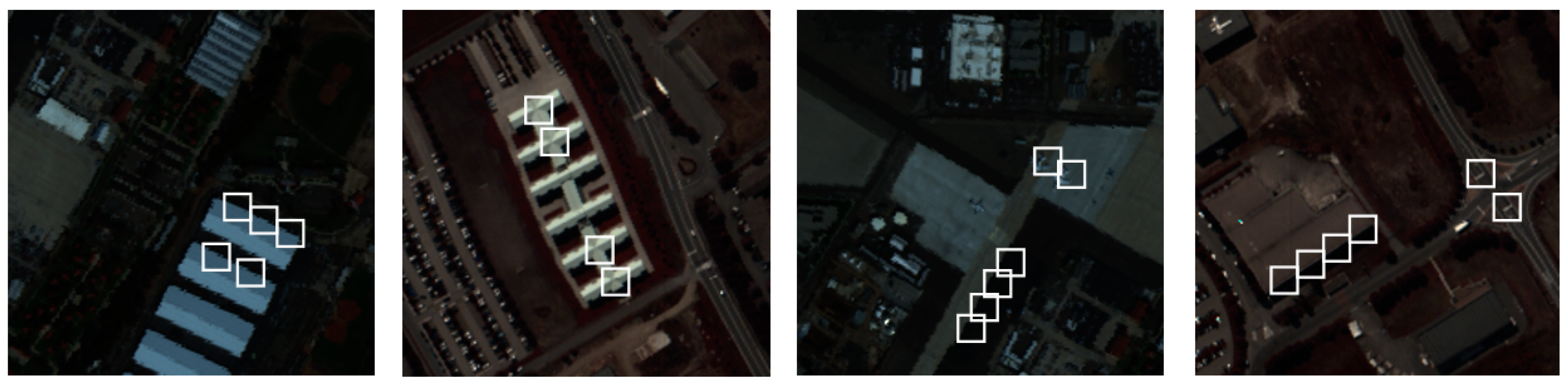
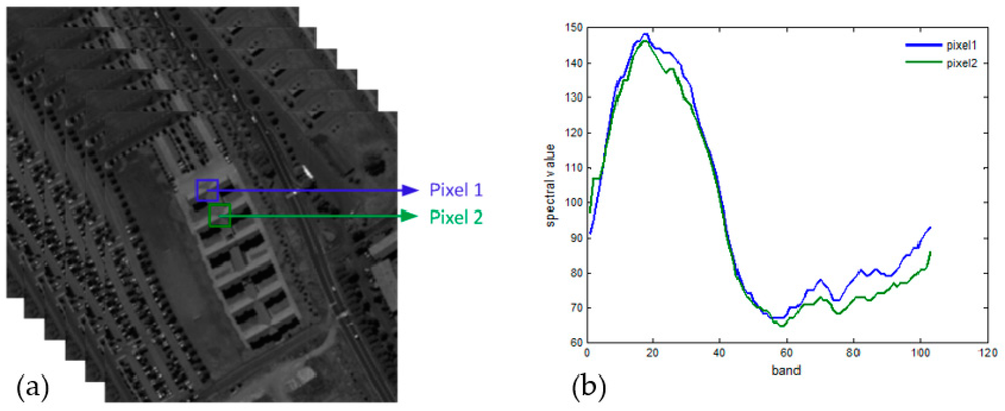
2.3. Non-Local Self-Similarity of Hyperspectral Images

Due to the information redundancy of HSIs, there may exist many similar or repeating structures in an image (as shown in Figure 1). These similar patches can provide extra information useful for preserving the details and has been extensively utilized in various kinds of image processing tasks such as denoising [34], fusion [35] and super-resolution [36,37]. The first algorithm using the non-local self-similarity property of an image is proposed for natural image denoising [34], in which each pixel of the noisy image is replaced by the weighted average of all pixels whose neighborhood is similar to the neighborhood of the current pixel. This methodology is also employed in a dictionary learning process for improved image fusion results [35]. In the super-resolution approaches [36,37], the non-local similarity of HSIs is employed to regularize the reconstructed image by using this property as a regularization term. This has been proven helpful for improving the quality of the reconstructed image.

Apart from the spatial self-similarity, non-local self-similarity of spectral vectors exists in HSIs. By exploiting the non-local self-similarity in the spectral domain, a new hyperspectral and multispectral image fusion approach is proposed in this paper. Rather than simply averaging the similar patches or pixels in hyperspectral images, this work jointly encodes the similar spectral vectors in the multispectral image, which can effectively avoid generating overly smooth results.

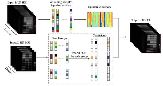
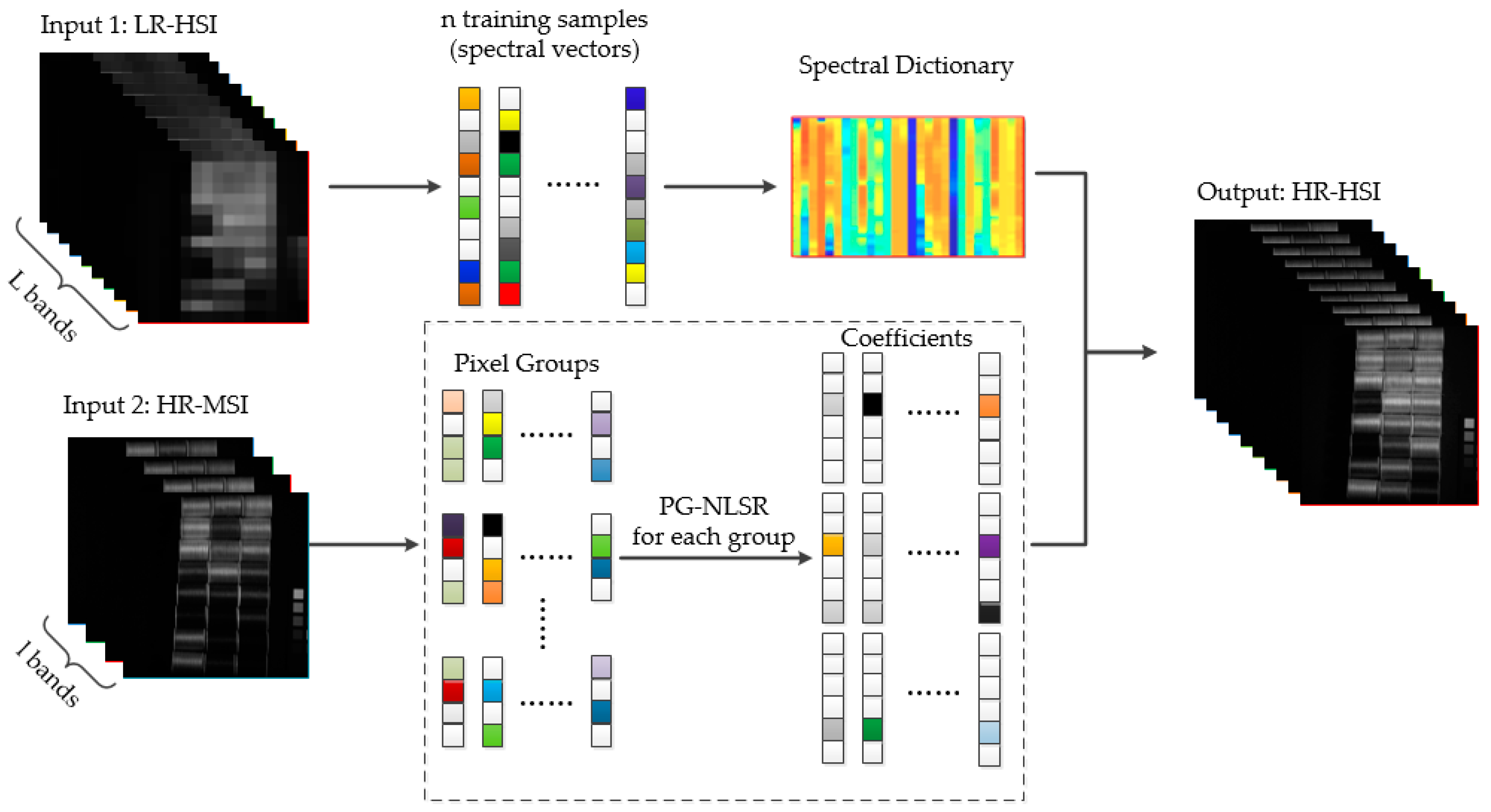
3. Proposed HSI Fusion Algorithm

3.1. Problem Formulation

Given a HSI with low spatial resolution (hereafter termed LR-HSI) $Y_h\in R^{m\times n\times L}$, and a high spatial resolution MSI (hereafter termed HR-MSI) $Y_m\in R^{M\times N\times l}$ of the same scene, this work aims to generate a HSI with high spatial resolution (hereafter, termed HR-HSI) $X_h\in R^{M\times N\times L}$. Here, $m$ and $M$ denote the respective image height, $n$ and $N$ the image width, and $l$ and $L$ the number of image bands. Note that there is the following relation: $m<M,n<N,l<L$.

For the convenience of implementation, the m × n × L dimensional LR-HSI $Y_h\in R^{m\times n\times L}$ is converted to L × mn dimensional form ${\overline{Y}}_h=[y_h(1,1),\cdots ,y_h(m,n)]\in R^{L\times mn}$, where each column of ${\overline{Y}}_h$ stands for one pixel in location $(i,j)$. Similarly, the HR-HSI $X_h\in R^{M\times N\times L}$ and the HR-MSI $Y_m\in R^{M\times N\times l}$ are transformed to ${\overline{X}}_h=[x_h(1,1),\cdots ,x_h(M,N)]\in R^{L\times MN}$ and ${\overline{Y}}_m=[y_m(1,1),y_m(1,2),\cdots y_m(M,N)]$ $\in R^{l\times MN}$, respectively.

Each pixel in the HR-MSI may be regarded as the spectral degradation of the desired pixel in HR-HSI:

$$y_m(i,j)=T{x}_h(i,j)$$

(4)

where $T\in R^{l\times L}$ is the spectral mapping matrix, which is determined by the relationship between the HSI sensor and the MSI sensor. Since in general $l<<L$, the reconstruction of ${\overline{X}}_h$ from ${\overline{Y}}_m$ is impossible without other prior knowledge. According to the LMM formulated in Equation (2), each pixel of the desired HR-HSI ${\overline{X}}_h$ can be decomposed as $x_h(i,j)=D{\alpha }_{ij}$. Considering the sparse constraint together with the linear mixing model, then the spatial resolution improvement problem can be solved by seeking the sparsest coefficient ${\alpha }_{ij}$ that satisfies the degradation equation $y_m(i,j)=TD{\alpha }_{ij}$:

$$\{\begin{array}{l}{\widehat{\alpha }}_{ij}=\underset{{\alpha }_{ij}}{\mathrm{arg\; min}}||{\alpha }_{ij}|{|}_0,s.t.||y_m(i,j)-TD{\alpha }_{ij}|{|}_2\le \epsilon \\ {\widehat{x}}_h(i,j)=D{\widehat{\alpha }}_{ij}\end{array}$$

(5)

The spectral dictionary $D$ is learned by applying an online dictionary learning algorithm [33] to a set of training samples, which are obtained by directly selecting column spectral vectors in ${\overline{Y}}_h\in R^{L\times mn}$. Once the spectral dictionary is known, the coefficient matrix can be computed by the proposed pixel group based non-local sparse representation technique, where a pixel group (PG) based strategy is adopted to implement the proposed method.

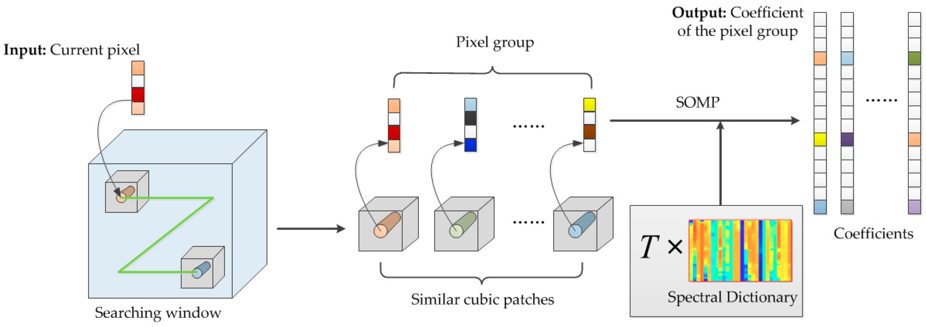
3.2. Pixel Group Based Non-Local Sparse Representation

The same scene of an HSI can contain many reoccurrences of the underlying materials that may exhibit similar spectral curves amongst materials of the same type (such as buildings, roads and lawns, etc.). The spectral reflectance of the central pixels in two similar cubic patches looks similar to each other (as shown in Figure 2). However, HR-HSI is not available during reconstruction. Thus, it is assumed that similar pixels in the HR-MSI are also similar in the HR-HSI at the same location. This is reasonable because the HR-MSI is obtained by the spectral down-sampling of HR-HSI. Therefore, the HR-MSI is employed to estimate the spectral self-similarity in HR-HSI. This spectral non-local image self-similarity is applied here to perform the pixel group based non-local sparse representation procedure, assuming that an ensemble of similar spectral vectors shares the same sparse pattern with different coefficients. The sparse codes of the desired HR-HSI are estimated by jointly encoding the similar pixels in each pixel group extracted from the HR-MSI. The pixel group based non-local sparse representation (hereafter termed PG-NLSR) procedure is illustrated in Figure 3.

More specifically, for each pixel $y_m(i,j)\in R^l$ of the HR-MSI, there are two main steps of the PG-NLSR: (1) constructing the pixel group of similar pixels; and (2) computing the sparse coefficients of the pixel group in Equation (1) through the simultaneous orthogonal matching pursuit (SOMP) [38] algorithm. Similar pixels are sought within a cubic searching window centered at $y_m(i,j)$. The selection of similar pixels is carried out by considering not only the spatial information ($w_1$), but also the spectral information ($w_2$). To do this, the similar weights between the current pixel $y_m(i,j)$ and pixel $y_m(s,t)$ in that searching window are first computed:

$$w(ij,st)=\frac{1}{Z}({\mu }_1{w}_1+{\mu }_2{w}_2)$$

(6)

$$w_1=\exp (-\frac{1}{L}{\displaystyle \sum _{k=1}^L||p_{ij}^k-p_{st}^k|{|}_{2,a}^2}/{h_1}^2)$$

(7)

$$w_2=\exp (-\mathrm{SAM}(y_m(i,j),y_m(s,t))/{h_2}^2)$$

(8)

where $||p_{ij}^k-p_{st}^k|{|}_{2,a}^2$ denotes the square of the Euclidean distance between the k-th band image patches $p_{ij}^k$ and $p_{st}^k$, which are centered at $y_m(i,j)$ and $y_m(s,t)$, respectively. $a>0$ denotes the standard deviation of the Gaussian kernel function and $Z$ is the normalizing constant. The parameters $h_1,h_2$ control the decay of the exponential function. SAM (Spectral Angle Mapper) denotes the spectral difference metric [39] between pixels $y_m(i,j)$ and $y_m(s,t)$. The first $b$ biggest $w(ij,st)$ are chosen and the corresponding $y_m(s,t)$ are selected as the similar pixels of $y_m(i,j)$. In addition, the similarity weight $w(ij,st)$ is also used to add a weight to the inner product when running the SOMP algorithm in order to obtain the sparse coefficients.

Let ${\overline{Y}}_m^{(i,j)}=[y_m(s_1,t_1),y_m(s_2,t_2),\cdots y_m(s_b,t_b)]$ be the pixel group consisting of $y_m(i,j)$ and its similar pixels, in which the first column is the current pixel $y_m(i,j)$. The SOMP algorithm is then employed to simultaneously encode the pixels in ${\overline{Y}}_m^{(i,j)}$ to obtain their non-local sparse coefficients, denoted by ${\widehat{A}}^{(i,j)}$. Then the spatial resolution improvement problem formulated in (5) can be converted to the following pixel group based non-local sparse representation problem:

$$\{\begin{array}{l}{\widehat{A}}^{(i,j)}=\underset{A^{(i,j)}}{\mathrm{arg\; min}}||A^{(i,j)}|{|}_{row,0}s.t.||{\overline{Y}}_m^{(i,j)}-TD{A}^{(i,j)}{||}_F\le \epsilon \\ {\widehat{\overline{X}}}_h^{(i,j)}=D{\widehat{A}}^{(i,j)}\end{array}$$

(9)

where $\epsilon$ denotes the model error and ${\widehat{A}}^{(i,j)}=[{\widehat{\alpha }}_{s_1{t}_1},{\widehat{\alpha }}_{s_2{t}_2}\cdots ,{\widehat{\alpha }}_{s_b{t}_b}]$ denotes the coefficient matrix. The notation $||\cdot |{|}_{row,0}$ is the norm counting the number of non-zero rows in the matrix. By integrating the estimated pixel groups $\text{{}{\widehat{\overline{X}}}_h^{(i,j)}|i=1,2,\cdots ,M;j=1,2,\cdots ,N\text{}}$, the desired HR-HSI is generated.

3.3. Algorithm

The proposed approach fuses the LR-HSI with a HR-MSI of the same scene. In the proposed algorithm, the LR-HSI is used to train the spectral dictionary, while the sparse coefficient matrix of each pixel group in HR-HSI is computed using the HR-MSI, guaranteeing that similar pixels are sparsely decomposed into the same subset of dictionary atoms. The proposed spatial and spectral fusion algorithm is illustrated in Figure 4. Firstly, the spectral dictionary is trained by performing an online dictionary learning algorithm to the given LR-HSI. Secondly, every pixel of the HR-MSI is extracted and a group of similar pixels of the current pixel is constructed. Thirdly, the pixels in the resulting group are jointly encoded using the SOMP algorithm. Finally, the spectral dictionary and the coefficients are combined to generate the required HR-HSI.

4. Experimental Results and Discussion

To verify the effectiveness of this proposed method, simulated experiments are carried out on two remote sensing datasets: (1) the AVRIS dataset; and (2) the ROSIS dataset.

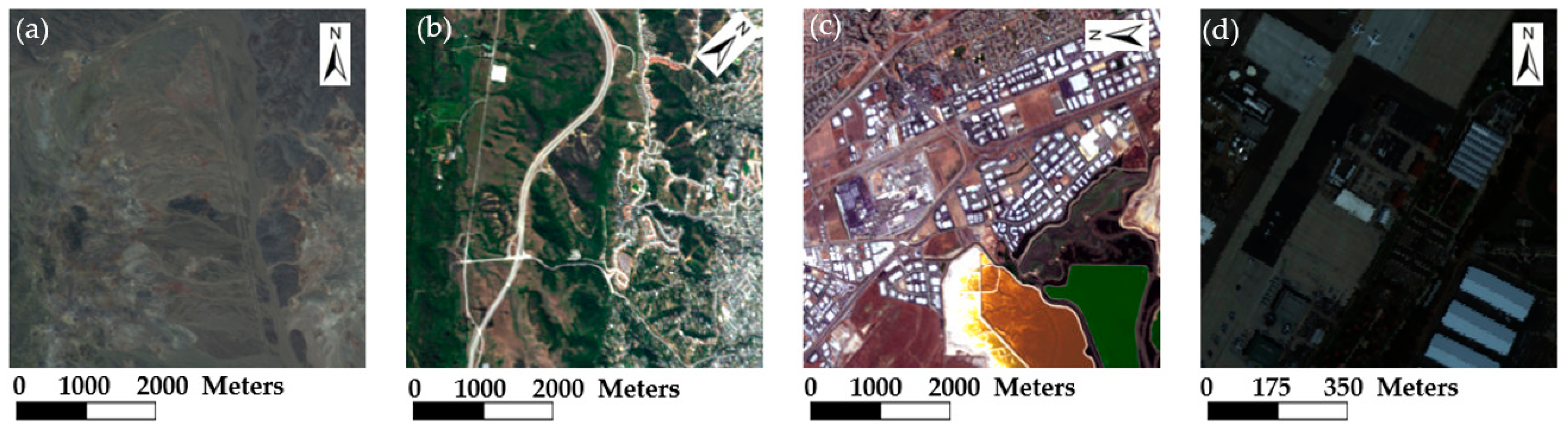
4.1. Experimental Setup

In the experimental studies, the proposed algorithm is applied to four 224-band HSIs taken by AVIRIS [40] and two HSIs taken by ROSIS [41], where the LR-HSI is fused with a simulated HR-MSI.

Some parameters used in the experimentation are set as follows: the number of atoms in spectral dictionary $k$ is 326 (the first atom of the spectral dictionary is the spatially-constant “DC” component); the number of similar pixels chosen in the non-local sparse representation procedure is set to $b=4$; the size of the cubic searching window is set to $5\times 5\times l$, while the size of the similar patch in Equation (7) is set to $3\times 3$; and the parameters ${\mu }_1,{\mu }_2$ in Equation (6) are empirically set as ${\mu }_1=0.7,{\mu }_2=0.3$. To further reduce the reconstruction error, the results are refined by the iterative back-projection technique. The performance of the proposed approach is compared with four fusion based schemes, namely the Matrix Factorization based approach (MF) [22], the Spatial and Spectral Fusion Model (SSFM) [23], the spatio-spectral sparse representation method, GSOMP [14], and the Bayesian Sparse Representation method (BSR) [24]. Additionally, we also test a simple Principal Component Analysis (PCA) [42] to obtain the basis in spectral dictionary D and then use Equation (2) to directly solve for the sparse coefficients. The performance of the different algorithms for the two data sets were tested on a PC with an Intel Core i5-4570 CPU @ 3.20 GHz and 8 GB RAM, using MATLAB R2014a.

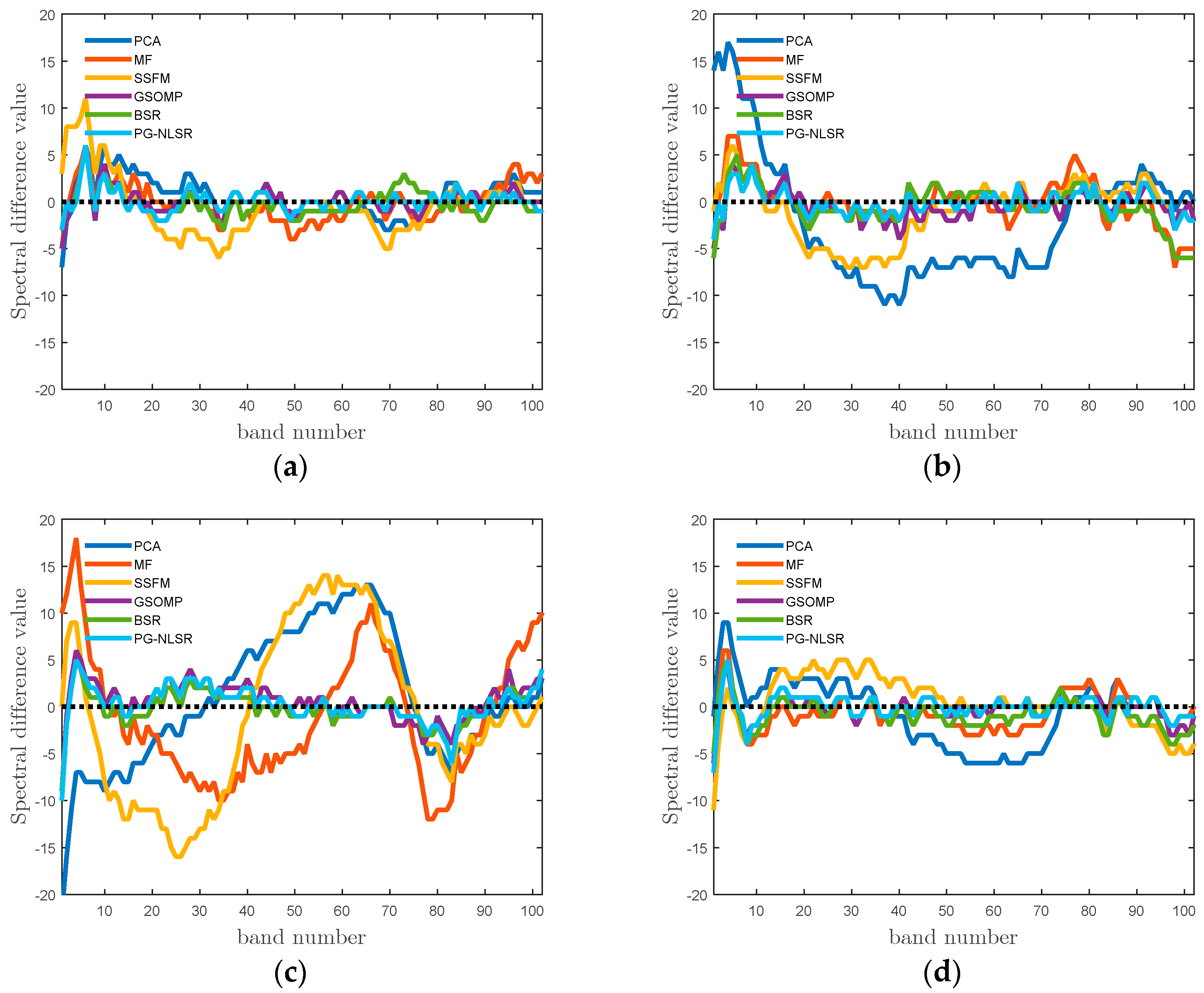
4.2. Performance Evaluation

To quantitatively assess the performance of the proposed spatial and spectral fusion algorithm, five quality indices are considered. The first one is the Root Mean Square Error (RMSE), which measures the difference between the estimated ${\widehat{\overline{X}}}_h$ and the original HR-HSI ${\overline{X}}_h$ (across all spectral bands) as follows:

$$\mathrm{RMSE}=\sqrt{\frac{||{\overline{X}}_h-{\widehat{\overline{X}}}_h|{|}_F^2}{M\times N\times L}}$$

(10)

The Peak Signal-to-Noise Ratio (PSNR) index is then easily computed via RMSE:

$$\mathrm{PSNR}=10{\log }_{10}(\frac{{\mathrm{MAX}}^2}{\mathrm{MSE}})$$

(11)

where $\mathrm{MSE}={\mathrm{RMSE}}^2$, and $\mathrm{MAX}$ represents the maximum value of ${\widehat{\overline{X}}}_h$. To measure the structural spatial details of the estimated images, the third index, the Average-Structural SIMilarity (A-SSIM), is calculated by averaging the SSIM metric among all spectral bands:

$$\mathrm{A}-\mathrm{SSIM}=\frac{1}{L}{\displaystyle \sum _{i=1}^L\frac{4{\mu }_{X_h^i}{\mu }_{{\widehat{X}}_h^i}{\sigma }_{X_h^i,{\widehat{X}}_h^i}}{({\mu }_{X_h^i}^2+{\mu }_{{\widehat{X}}_h^i}^2)({\sigma }_{X_h^i}^2+{\sigma }_{{\widehat{X}}_h^i}^2)}}$$

(12)

where $\mu$, ${\sigma }^2$ and $\sigma$ are the mean, variance and covariance of the corresponding image matrices, respectively; and $X_h^i$ and ${\widehat{X}}_h^i$ denote the $i$th band of $X_h$ and ${\widehat{X}}_h$, respectively. To measure the spectral reconstruction performance, the Spectral Angel Mapper (SAM) [43] is computed. The SAM index is defined as the spectral angle between the estimated pixel ${\widehat{x}}_h(i,j)$ and the original pixel $x_h(i,j)$:

$$\mathrm{SAM}=\arccos \left(\frac{<x_h(i,j),{\widehat{x}}_h(i,j)>}{||x_h(i,j)|{|}_2\cdot ||{\widehat{x}}_h(i,j)|{|}_2}\right)$$

(13)

and the final SAM is obtained by averaging the SAMs of all pixels in an image. The last index is the relative dimensionless global error in synthesis (ERGAS) [43], which is defined as:

$$\mathrm{ERGAS}=100\frac{d_h}{d_l}\sqrt{\frac{1}{L}{\displaystyle \sum _{l=1}^L{\left(\frac{\mathrm{RMSE}(l)}{\mu (l)}\right)}^2}}$$

(14)

where $d_h/d_l$ is the ratio between the pixel sizes of the HR-HSI and the LR-HSI. The best value of RMSE, SAM and ERGAS are zero; the best value of A-SSIM is 1; and the best value of PSNR is $+\infty$. The RMSE, A-SSIM and PSNR indices show the degree of spatial similarity between the estimated image and the corresponding original HR-HSI, with the SAM index showing the degree of spectral similarity, while the ERGAS index reflects a global picture of the quality of the fused image.

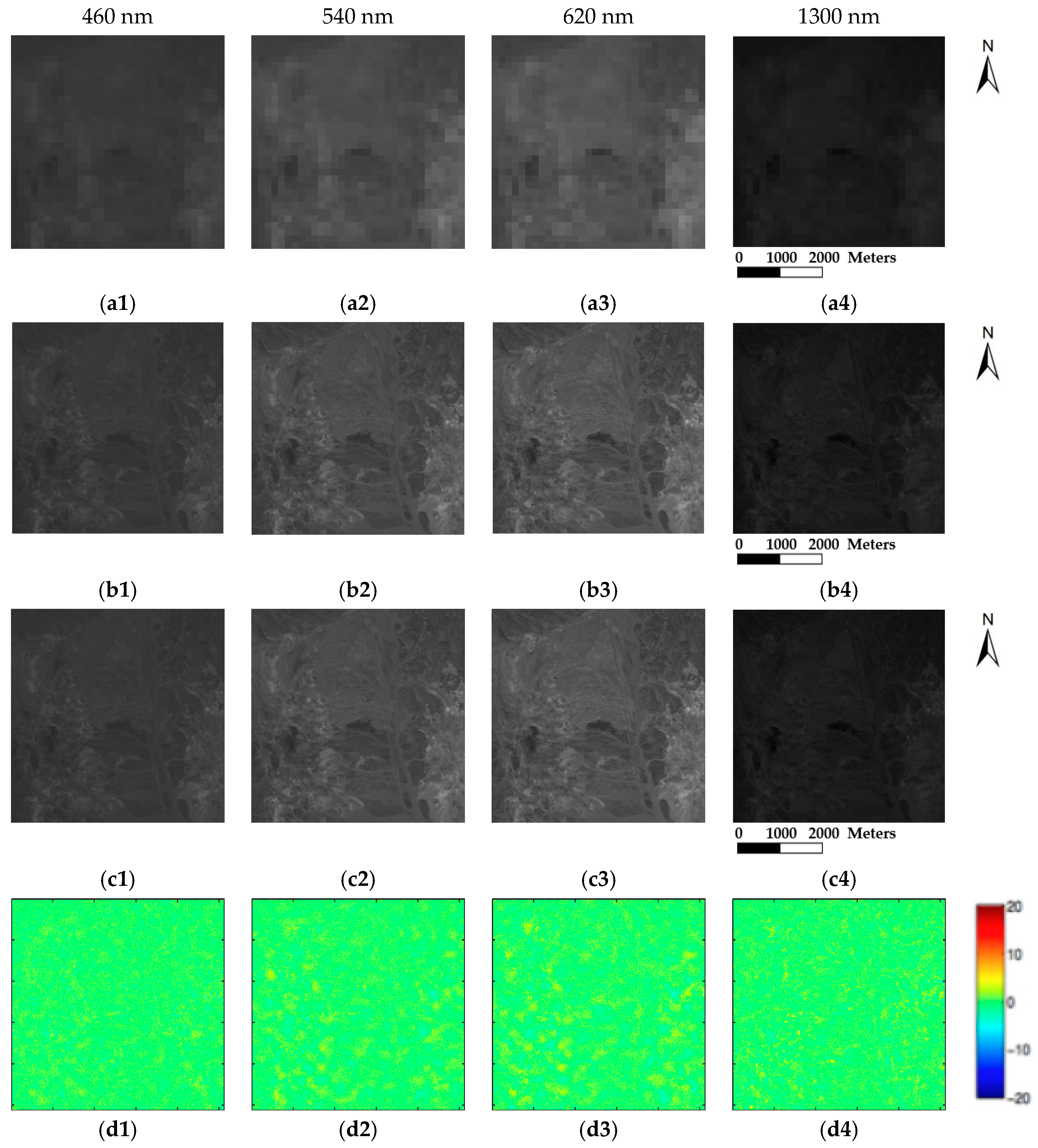
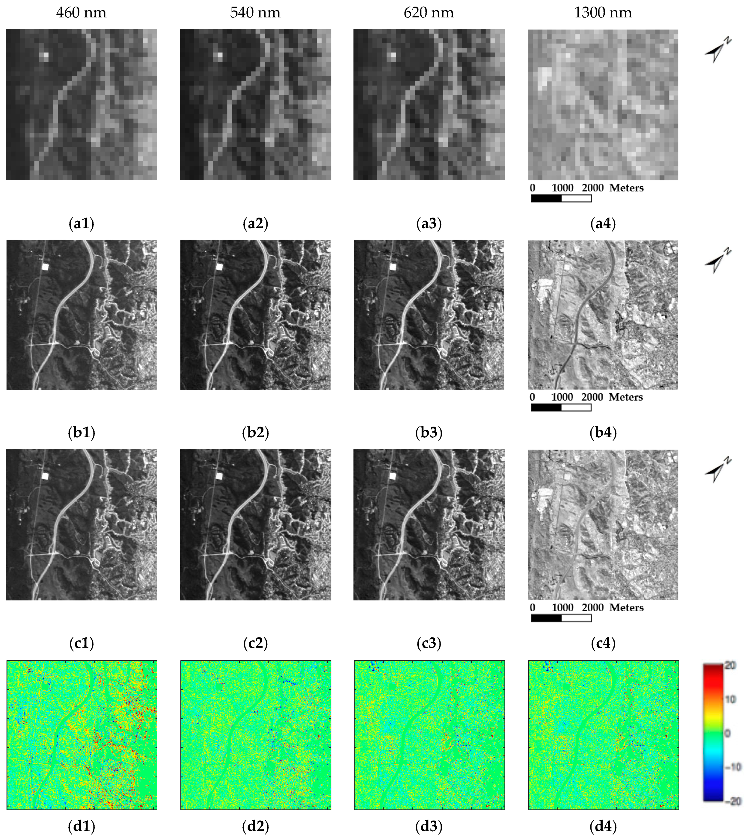
4.3. Experiments on AVIRIS Dataset

In this section, we apply the proposed PG-NLSR algorithm to four 224-band remote sensing HSIs, which are taken by the Airborne Visible/Infrared Imaging Spectrometer (AVIRIS) sensor [44]. The first image Cuprite was taken over Cuprite, NV, in 1997 with an original spatial resolution at 20 m. The second, Jasper-Ridge, was acquired over Jasper Ridge, CA, USA, in 1994, with a spatial resolution of 20 m. The third image Moffett-Field was acquired over Moffett Field, CA, USA, in 1994 by Jet Propulsion Laboratory at a 20 m resolution. The last image San Diego, acquired in 2002, covers a naval air station in San Diego, CA, USA, with a spatial resolution of 3.5 m. After removing the noisy and water vapor absorption bands, four sub-images (shown in Figure 5) of size 256 × 256 × 189 are selected and used as the original HR-HSIs.

The LR-HSIs are simulated by first applying a 5 × 5 Gaussian kernel with standard deviation 2.5 to the original HR-HSIs and then downsampling along both horizontal and vertical directions with a scaling factor of 8 (i.e., the spatial resolution of the four simulated LR-HSIs is 160 m, 160 m, 160 m and 28 m, respectively). The Gaussian white noise is added to the LR-HSIs with a standard deviation 0.5. The HR-MSIs are generated by integrating the bands of the original HR-HSIs with uniform spectral response functions corresponding to Landsat TM bands 1–5 and 7 at 20 m or 3.5 m resolution, which cover the 450–520, 520–600, 630–690, 760–900, 1550–1750 and 2080–2350 nm regions, respectively [45]. The estimated HR-HSIs of 460 nm, 540 nm, 620 nm and 1300 nm bands using the proposed approach are shown in Figure 6 and Figure 7, where the fourth row shows the error image of these bands. Here, the error images are generated by computing the differences between the estimated HR-HSI and the original HR-HSI, on a pixel by pixel strategy. Quantitative evaluation measures for different enhancement approaches are compared in

Table 1. Evaluation assessments of different fusion schemes for remote sensing HSIs.

Images	Index	PCA [42]	MF [22]	SSFM [23]	GSOMP [14]	BSR [24]	PG-NLSR
Cuprite	RMSE	1.6760	0.5498	0.7113	0.4665	0.3033	0.2845
	PSNR	43.6453	53.3265	51.0896	54.7540	58.4946	59.0488
	A-SSIM	0.9845	0.9907	0.9785	0.9935	0.9931	0.9946
	SAM	2.2749	1.2558	2.2691	1.0409	1.1676	0.8559
	ERGAS	6.2879	2.1209	2.6783	1.0535	0.8973	1.0636
Jasper-Ridge	RMSE	11.4688	7.6531	7.2652	4.5126	5.7721	3.7483
	PSNR	26.9405	30.4541	30.9058	35.0422	32.9042	36.6542
	A-SSIM	0.8733	0.8704	0.9240	0.9178	0.9160	0.9264
	SAM	5.8845	5.4792	4.3946	3.8501	4.0804	3.6892
	ERGAS	1.6518	1.4547	1.1428	1.1183	1.0054	1.0036
Moffett-Field	RMSE	15.9288	8.2029	7.7466	5.5780	4.1883	4.1833
	PSNR	24.0871	29.8514	30.3486	33.2012	35.6901	35.7005
	A-SSIM	0.9030	0.8736	0.8668	0.9296	0.9234	0.9371
	SAM	8.8194	7.6709	8.4644	4.3319	5.0234	3.7269
	ERGAS	2.0839	1.4930	1.5145	1.0245	0.9084	0.8275
San Diego	RMSE	7.9201	4.2662	3.1145	1.6225	1.2230	0.8681
	PSNR	30.1562	35.5300	38.2631	43.9273	46.3823	49.3598
	A-SSIM	0.7670	0.9365	0.9746	0.9663	0.9796	0.9803
	SAM	5.4728	2.2006	1.7335	0.8499	0.6451	0.7305
	ERGAS	4.1063	1.9276	1.0549	0.9950	0.4635	0.5877

. The proposed method PG-NLSR outperformed all compared methods except BSR which for a couple of indices has better results in images Cuprite and San Diego. PG-NLSR has generated most of the best results which are indicated in bold.

Qualitatively, the estimated HR-HSIs shown in Figure 6c and Figure 7c are very close to the original HR-HSIs in Figure 6b and Figure 7b. Error image (Figure 6d) for the Cuprite image show very minor differences between the estimated HR-HSI (Figure 6c) and the original image (Figure 6b). The estimation error is concentrated mainly around the areas where pixels change rapidly. However, higher errors can be found in Figure 7d in boundary of smaller objects and transitional land cover types. Figure 8 shows the visual results of the Moffett-field image. The spatial details of the fusion images among different algorithms are illustrated. The black box in Figure 8a shows the area-of-interest that were enlarged and compared in Figure 8c–h. Both buildings and roads can be clearly seen in all fused images. However, the details in the lower-left corner of Figure 8h are cleaner and the color of Figure 8h has a better resemblance to the original HR-HSI of Figure 8b. Quantitative comparisons shown in Table 1 indicate that the performance of the proposed scheme is better than that of the rest. This is because the proposed pixel group based non-local sparse representation technique makes full use of the similar spectral vectors within a certain searching window.

The number of similar pixels chosen in a pixel group (b) is an important parameter in the proposed PG-NLSR, which controls the balance between the fusion accuracy and the computational efficiency. The performance (RMSE) and running time (in seconds) of different values for parameter b on image Cuprite is shown in Figure 9. It can be seen from the curve that when more similar pixels are selected, the fusion results will be better, owing to that more extra information are provided and a more optimal sparse representation of a given pixel is found. However, the computational cost will inevitably increase rapidly as more similar pixels are selected. As shown in Figure 9a, the RMSE assessment decreases rapidly before b = 4, and the decrease becomes much slower after that point. By trading off the fusion accuracy and the computational efficiency, we select the four most similar pixels from the total of 25 pixels in the cubic searching window.

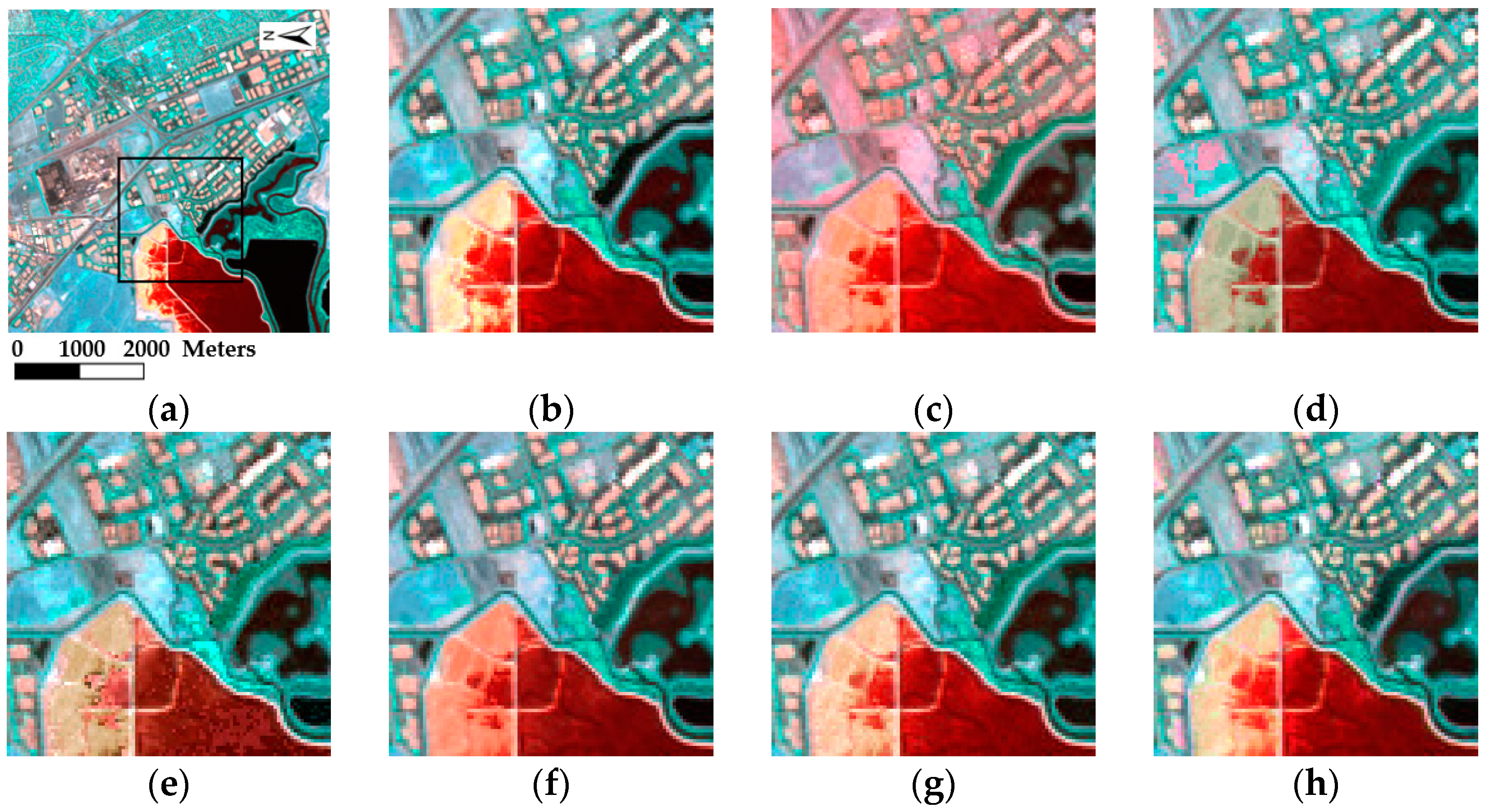
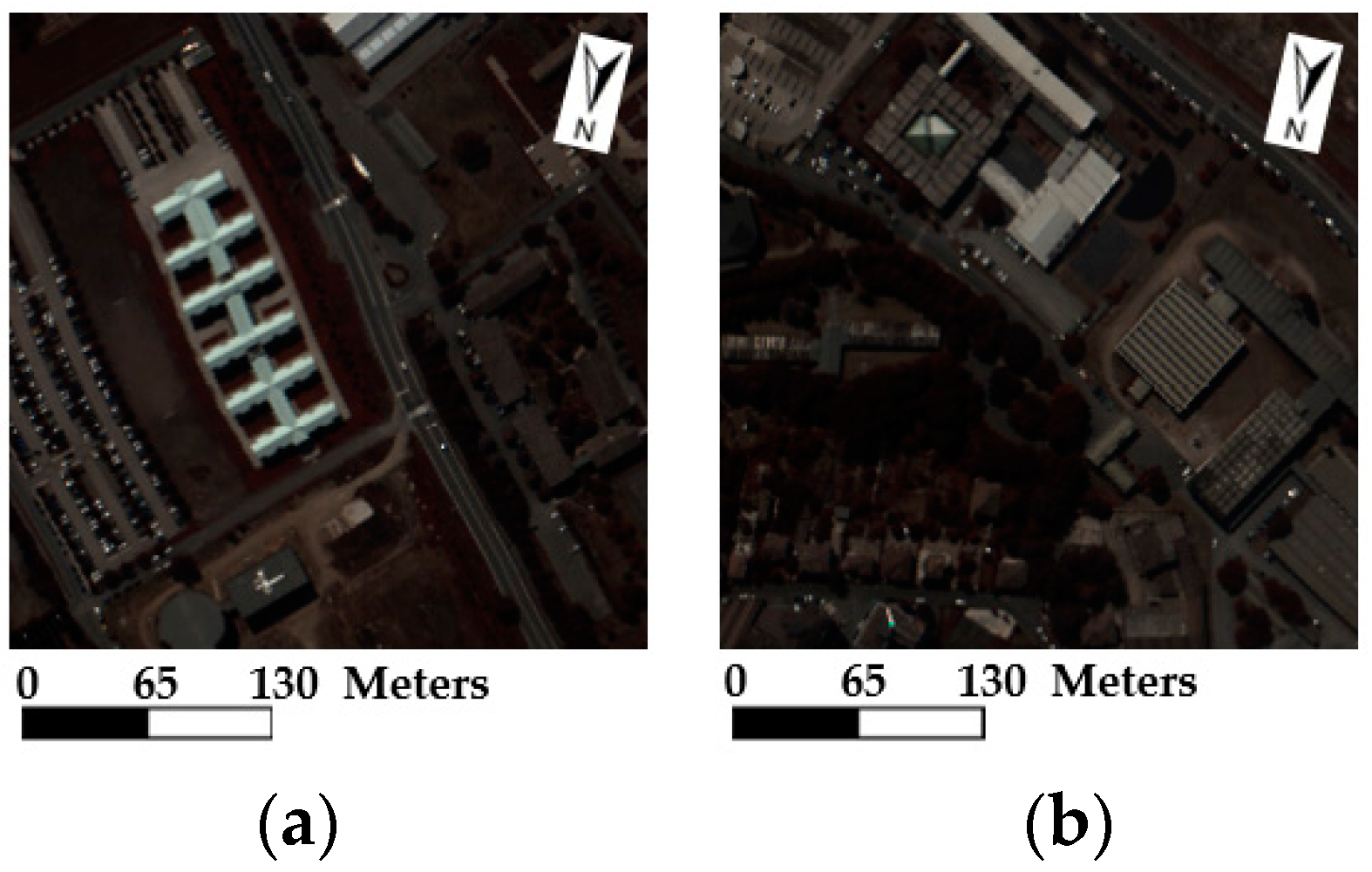
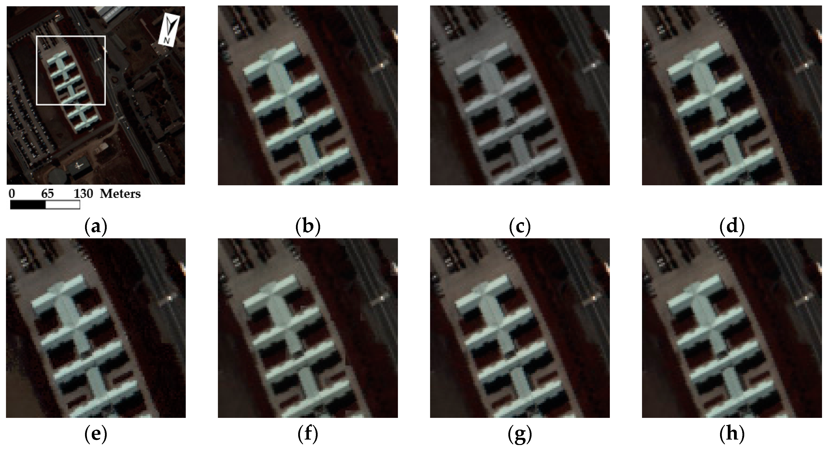
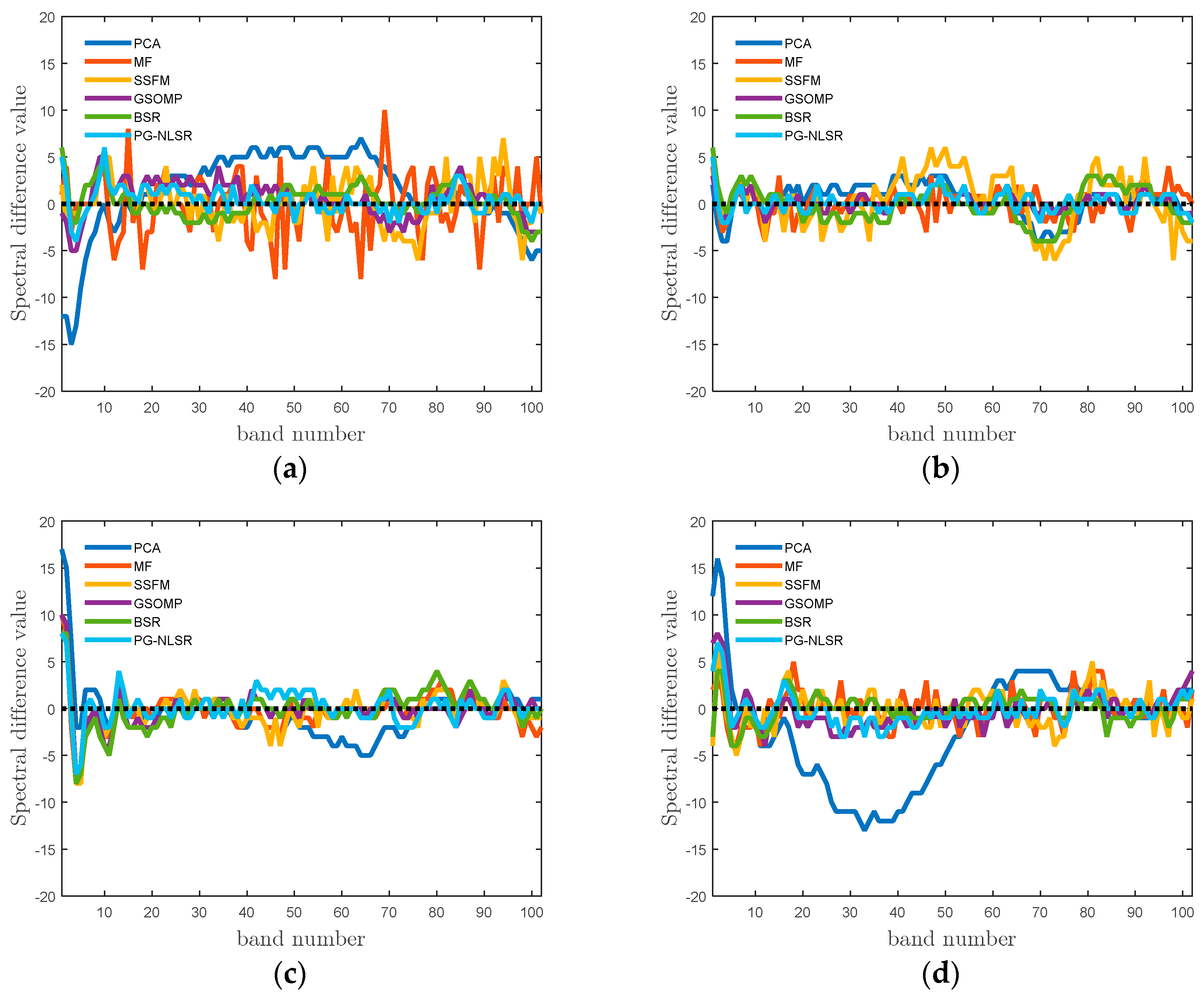
4.4. Experiments on ROSIS Dataset

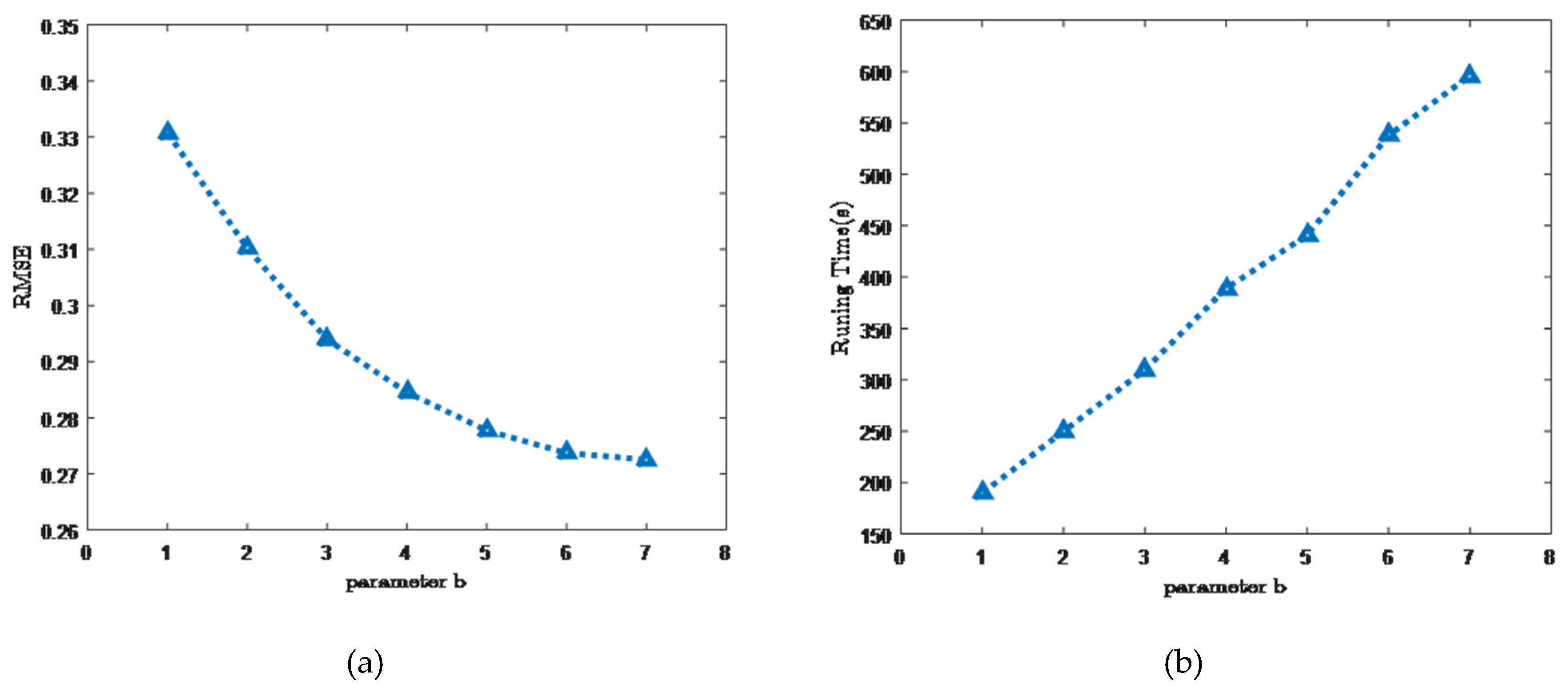
To further demonstrate the proposed method can be effective with concurrent sensors, we test the fusion with LR-HSI and Sentinel 2A-like HR-MSI. The experiment makes use of a 102-band HSI (Pavia Centre) and a 103-band HSI (Pavia University) as shown in Figure 10 with an original spatial resolution of 1.3 m. These two images were acquired in 2001 by the ROSIS (Reflective Optics System Imaging Spectrometer) optical sensor over the center area and the University of Pavia, Italy. The flight was operated by the Deutsches Zentrum für Luft- und Raumfahrt (DLR, the German Aerospace Agency) in the framework of the HySens project, managed and sponsored by the European Union. The noisy and water vapor absorption bands have been removed from the initially 115 bands. A region of 256 × 256 pixels are selected and used as the original HR-HSIs, which is then blurred by a 5 × 5 Gaussian kernel with standard deviation 2.5. Then the images were down-sampled with the scale factors (denoted by S) of 4, 8 and 16 to simulate the LR-HSIs in corresponding spatial resolutions of 5.2 m, 10.4 m and 20.8 m, respectively. The Gaussian white noise is added to the LR-HSIs with a standard deviation 0.5. The HR-MSI is generated by filtering the HR-HSI with Sentinel2A-like spectral responses (bands 1–8). The reflectance spectral responses of the simulated bands used for the fusion are depicted in Figure 11.

The visual results of different approaches at scale factor = 8 are presented in Figure 12, while the quantitative evaluation measures are compared in

Table 2. Evaluation assessments for Pavia Centre HSI over different scale factors.

Method	PCA [42]	MF [22]	SSFM [23]	GSOMP [14]	BSR [24]	PG-NLSR
S = 4
RMSE	2.7352	1.6695	2.2580	1.0116	0.7201	0.7074
PSNR	39.3909	43.6790	41.0563	48.0309	50.9825	51.1380
A-SSIM	0.9239	0.9604	0.9509	0.9783	0.9834	0.9856
SAM	6.4478	3.7423	4.2193	3.1318	2.4157	2.3337
ERGAS	4.0682	2.1829	2.4277	0.9209	1.2902	1.3564
S = 8
RMSE	2.7766	1.8995	2.5754	1.0385	0.9034	0.7491
PSNR	39.2604	42.5581	39.9138	47.8028	49.0129	50.6400
A-SSIM	0.9226	0.9481	0.9353	0.9770	0.9774	0.9835
SAM	6.5122	4.2119	4.4572	3.1750	2.9190	2.5365
ERGAS	2.0528	1.2366	1.4232	0.9522	0.7687	0.7266
S = 16
RMSE	2.8523	2.1191	2.6062	1.1919	0.9364	0.9272
PSNR	39.0270	41.6079	39.8108	46.6057	48.7015	48.7869
A-SSIM	0.9203	0.9330	0.9192	0.9726	0.9793	0.9792
SAM	6.6424	5.8780	6.3314	3.4892	2.9286	3.0127
ERGAS	1.0456	0.8301	1.0255	0.5459	0.3917	0.4312

and

Table 3. Evaluation assessments for Pavia University HSI over different scale factors.

Method	PCA [42]	MF [22]	SSFM [23]	GSOMP [14]	BSR [24]	PG-NLSR
S = 4
RMSE	3.5179	1.6974	1.9599	1.1712	0.7582	0.7179
PSNR	37.2052	43.5353	42.2863	46.7582	50.5351	51.0097
A-SSIM	0.9270	0.9734	0.9423	0.9765	0.9842	0.9859
SAM	6.4194	3.0905	4.7297	2.8398	2.2157	2.1693
ERGAS	4.9933	1.8510	2.9534	1.8718	1.2416	1.2823
S = 8
RMSE	3.5091	1.9775	2.4717	1.6876	0.8690	0.8518
PSNR	37.2269	42.2087	40.2707	43.5855	49.3501	49.5245
A-SSIM	0.9257	0.9536	0.9121	0.9684	0.9829	0.9837
SAM	6.4898	3.7624	5.7924	3.2346	2.3855	2.3787
ERGAS	2.5084	1.2374	1.8591	1.1668	0.6650	0.7184
S = 16
RMSE	3.5297	2.2620	2.7045	2.1770	1.1513	1.1959
PSNR	37.1760	41.0409	39.4890	41.3736	46.9070	46.5769
A-SSIM	0.9240	0.9589	0.9370	0.9596	0.9665	0.9786
SAM	6.5875	3.9974	5.6065	3.9253	3.1329	2.9365
ERGAS	1.2658	0.6532	0.9143	0.7283	0.4312	0.4530

. The average running time (in seconds) of different algorithms is shown in

Table 4. Average Computational Time (in seconds) of Different Algorithms.

Data Set	PCA [42]	MF [22]	SSFM [23]	GSOMP [14]	BSR [24]	PG-NLSR
AVIRIS	7	31	30	151	3229	493
ROSIS	6	29	29	116	2110	472

. The spectral reflectance difference value of four single pixels ((a) (50, 50), (b) (100, 100), (c) (150, 150), and (d) (180, 200)) shown in Figure 13 and Figure 14 compares the estimation error between the original HR-HSIs and the resulting images of different fusion algorithms. The results show that the proposed approach has the smallest difference when compared to the actual pixel value.

As scale factor increases, the information lost in the down-sampling procedure rises rapidly, and the resolution enhancement task will be much more difficult. Qualitative and quantitative assessments have both demonstrated the effectiveness of the proposed PG-NLSR fusion method at different scale factors. Qualitative comparisons depicted in Figure 12 indicate that the estimated HR-HSI shown in Figure 12h seems no difference with the original high spatial resolution data in Figure 12b, while the quantitative indices in Table 2 and Table 3 show that the proposed PG-NLSR technique outperforms the other fusion methods. As shown in Table 2 and Table 3, The Bayesian Sparse Representation based method [24] performs slightly better at some indices, but the computing time is unavoidably much higher as a consequence (shown in Table 4).

4.5. Discussion

From the above experimental results, it can be seen that the proposed approach outperforms the other five fusion based methods, with acceptable running time. In particular, for the AVIRIS dataset, on average, the RMSE of the proposed method decreases 0.6 when compared with that of BSR, and in comparison with the GSOMP, SSFM, MF and the PCA algorithms, the improvement is even more significant (with a reduction of 6.98, 2.9, 2.44 and 0.77 in RMSE, respectively). For the ROSIS dataset, the BSR-based method performs slightly better at some indices where the scale factor is large, but this is at the cost of a significant amount of time (to implement the Bayesian learning and coding procedures).

The superiority of the proposed approach is owing to the employment of pixel group based non-local sparse representation, where a group of similar pixels are encoded simultaneously. This strategy supports the encoding procedure to utilize the information provided by not only the current pixel itself but also those similar to it. Of course, how to choose similar pixels in a group is an important process that may affect the fusion outcome. In this work, the degree of similarity of two pixels is measured by a weighted average of the spatial similarity and the spectral similarity, with the weights empirically set to 0.7 for the former and 0.3 for the latter. However, this strategy does not take the structural property of HSI into consideration. Besides, the fixed weights may not be suitable for all images. Therefore, to achieve more accurate fusion results, it is interesting to investigate whether a more appropriate similarity measure can be devised, but this remains as further research.

It is also interesting to note that whilst the experimental results demonstrate the effectiveness of the proposed approach, the computational cost is generally quite high when the pixel group based non-local sparse representation technique is used. Methods that could help expedite the required computation would be very helpful. Currently, a spectral dictionary is trained for each input HIS, which is time consuming. Thus, learning an off-line dictionary that could be used for a large amount of images would be another interesting improvement of this research.

5. Conclusions

In this work, a spatial and spectral image fusion approach with non-local sparse representation has been presented. The proposed PG-NLSR approach fuses an LR-HSI with an HR-MSI of the same scene to improve the spatial resolution of the LR-HSI. It learns a spectral dictionary using the LR-HSI, and applies the pixel group based non-local sparse representation technique to obtain the sparse code of a desirable high spatial resolution image. In so doing, the proposed work exploits the non-local self-similarity of hyperspectral images. In addition, the present research allows for the selection of similar pixels to be carried out using not only the spectral information, but also the spatial information. The approach has been systematically compared with a number of existing fusion based techniques. The experimental comparisons involve two remote sensing datasets, demonstrating the effectiveness of this work.

References

1. Bioucas-Dias, J.M.; Plaza, A.; Camps-Valls, G.; Scheunders, P.; Nasrabadi, N.; Chanussot, J. Hyperspectral remote sensing. data analysis and future challenges. IEEE Geosci. Remote Sens. Mag. 2013, 1, 6–36. [Google Scholar] [CrossRef]
2. Patel, R.C.; Joshi, M.V. Super-resolution of hyperspectral images: Use of optimum wavelet filter coefficients and sparsity regularization. IEEE Trans. Geosci. Remote Sens. 2015, 53, 1728–1736. [Google Scholar] [CrossRef]
3. Feng, R.; Zhong, Y.; Wu, Y.; He, D.; Xu, X.; Zhang, L. Nonlocal total variation subpixel mapping for hyperspectral remote sensing imagery. Remote Sens. 2016, 8. [Google Scholar] [CrossRef]
4. Yokoya, N.; Yairi, T.; Iwasaki, A. Coupled nonnegative matrix factorization unmixing for hyperspectral and multispectral data fusion. IEEE Trans. Geosci. Remote Sens. 2012, 50, 528–537. [Google Scholar] [CrossRef]
5. Loncan, L.; de Almeida, L.B.; Bioucas-Dias, J.M.; Briottet, X.; Chanussot, J.; Dobigeon, N.; Fabre, S.; Liao, W.; Licciardi, G.A.; Simoes, M. Hyperspectral pansharpening: A review. IEEE Geosci. Remote Sens. Mag. 2015, 3, 27–46. [Google Scholar] [CrossRef]
6. Shettigara, V. A generalized component substitution technique for spatial enhancement of multispectral images using a higher resolution data set. Photogramm. Eng. Remote Sens. 1992, 58, 561–567. [Google Scholar]
7. Choi, M. A new intensity-hue-saturation fusion approach to image fusion with a tradeoff parameter. IEEE Trans. Geosci. Remote Sens. 2006, 44, 1672–1682. [Google Scholar] [CrossRef]
8. Pradhan, P.S.; King, R.L.; Younan, N.H.; Holcomb, D.W. Estimation of the number of decomposition levels for a wavelet-based multiresolution multisensor image fusion. IEEE Trans. Geosci. Remote Sens. 2006, 44, 3674–3686. [Google Scholar] [CrossRef]
9. Robinson, G.D.; Gross, H.N.; Schott, J.R. Evaluation of two applications of spectral mixing models to image fusion. Remote Sens. Environ. 2000, 71, 272–281. [Google Scholar] [CrossRef]
10. Zurita-Milla, R.; Clevers, J.G.; Schaepman, M.E. Unmixing-based Landsat TM and MERIS FR data fusion. IEEE Geosci. Remote Sens. Lett. 2008, 5, 453–457. [Google Scholar] [CrossRef] [Green Version]
11. Lanaras, C.; Baltsavias, E.; Schindler, K. Hyperspectral super-resolution by coupled spectral unmixing. In Proceedings of the IEEE International Conference on Computer Vision, Santiago, Chile, 7–13 December 2015; pp. 3586–3594.
12. Nezhad, Z.H.; Karami, A.; Heylen, R.; Scheunders, P. Fusion of hyperspectral and multispectral images using spectral unmixing and sparse coding. IEEE J. Sel. Top. Appl. Earth Obs. Remote Sens. 2016, 9, 2377–2389. [Google Scholar] [CrossRef]
13. Bieniarz, J.; Müller, R.; Zhu, X.X.; Reinartz, P. Hyperspectral image resolution enhancement based on joint sparsity spectral unmixing. In Proceedings of the IEEE Geoscience and Remote Sensing Symposium, Quebec City, QC, Canada, 13–18 July 2014; pp. 2645–2648.
14. Akhtar, N.; Shafait, F.; Mian, A. Sparse spatio-spectral representation for hyperspectral image super-resolution. In Proceedings of the European Conference on Computer Vision, Zurich, Switzerland, 6–12 September 2014; pp. 63–78.
15. Wycoff, E.; Chan, T.H.; Jia, K.; Ma, W.K.; Ma, Y. A non-negative sparse promoting algorithm for high resolution hyperspectral imaging. In Proceedings of the IEEE International Conference on Acoustics, Speech and Signal Processing, Vancouver, BC, Canada, 26–31 May 2013; pp. 1409–1413.
16. Iordache, M.D.; Bioucas-Dias, J.M.; Plaza, A. Sparse unmixing of hyperspectral data. IEEE Trans. Geosci. Remote Sens. 2011, 49, 2014–2039. [Google Scholar] [CrossRef]
17. Li, S.; Yin, H.; Fang, L. Remote sensing image fusion via sparse representations over learned dictionaries. IEEE Trans. Geosci. Remote Sens. 2013, 51, 4779–4789. [Google Scholar] [CrossRef]
18. Guo, M.; Zhang, H.; Li, J.; Zhang, L.; Shen, H. An online coupled dictionary learning approach for remote sensing image fusion. IEEE J. Sel. Top. Appl. Earth Obs. Remote Sens. 2014, 7, 1284–1294. [Google Scholar] [CrossRef]
19. Dong, W.; Fu, F.; Shi, G.; Cao, X.; Wu, J.; Li, G.; Li, X. Hyperspectral image super-resolution via non-negative structured sparse representation. IEEE Trans. Image Process. 2016, 25, 2337–2352. [Google Scholar] [CrossRef] [PubMed]
20. Wei, Q.; Bioucas-Dias, J.; Dobigeon, N.; Tourneret, J.Y. Hyperspectral and multispectral image fusion based on a sparse representation. IEEE Trans. Geosci. Remote Sens. 2015, 53, 3658–3668. [Google Scholar] [CrossRef]
21. Song, H.; Huang, B.; Liu, Q.; Zhang, K. Improving the spatial resolution of Landsat TM/ETM+ through fusion with SPOT5 images via learning-based super-resolution. IEEE Trans. Geosci. Remote Sens. 2015, 53, 1195–1204. [Google Scholar] [CrossRef]
22. Kawakami, R.; Matsushita, Y.; Wright, J.; Ben-Ezra, M.; Tai, Y.W.; Ikeuchi, K. High-resolution hyperspectral imaging via matrix factorization. In Proceedings of the IEEE Conference on Computer Vision and Pattern Recognition, Colorado Springs, CO, USA, 20–25 June 2011; pp. 2329–2336.
23. Huang, B.; Song, H.; Cui, H.; Peng, J.; Xu, Z. Spatial and spectral image fusion using sparse matrix factorization. IEEE Trans. Geosci. Remote Sens. 2014, 52, 1693–1704. [Google Scholar] [CrossRef]
24. Akhtar, N.; Shafait, F.; Mian, A. Bayesian sparse representation for hyperspectral image super resolution. In Proceedings of the IEEE Conference on Computer Vision and Pattern Recognition, Boston, MA, USA, 7–12 June 2015; pp. 3631–3640.
25. Wright, J.; Ma, Y.; Mairal, J.; Sapiro, G.; Huang, T.S.; Yan, S. Sparse representation for computer vision and pattern recognition. Proc. IEEE 2010, 98, 1031–1044. [Google Scholar] [CrossRef]
26. Pati, Y.C.; Rezaiifar, R.; Krishnaprasad, P. Orthogonal matching pursuit: Recursive function approximation with applications to wavelet decomposition. In Proceedings of the 27th Asilomar Conference on Signals, Systems and Computers, Pacific Grove, CA, USA, 1–3 November 1993; pp. 40–44.
27. Donoho, D.L.; Tsaig, Y.; Drori, I.; Starck, J.L. Sparse solution of underdetermined systems of linear equations by stagewise orthogonal matching pursuit. IEEE Trans. Inf. Theory 2012, 58, 1094–1121. [Google Scholar] [CrossRef]
28. Chen, S.S.; Donoho, D.L.; Saunders, M.A. Atomic decomposition by basis pursuit. SIAM Rev. 2001, 43, 129–159. [Google Scholar] [CrossRef]
29. Tibshirani, R. Regression shrinkage and selection via the lasso: A retrospective. J. R. Stat. Soc. Ser. B Stat. Methodol. 2011, 73, 273–282. [Google Scholar] [CrossRef]
30. Daubechies, I.; Defrise, M.; De Mol, C. An iterative thresholding algorithm for linear inverse problems with a sparsity constraint. Commun. Pure Appl. Math. 2004, 57, 1413–1457. [Google Scholar] [CrossRef]
31. Şımşek, M.; Polat, E. The effect of dictionary learning algorithms on super-resolution hyperspectral reconstruction. In Proceedings of the XXV International Conference on Information, Communication and Automation Technologies, Sarajevo, Bosnia and Herzegovina, 29–31 October 2015; pp. 1–5.
32. Aharon, M.; Elad, M.; Bruckstein, A. K-svd: An algorithm for designing overcomplete dictionaries for sparse representation. IEEE Trans. Signal Proc. 2006, 54, 4311–4322. [Google Scholar] [CrossRef]
33. Mairal, J.; Bach, F.; Ponce, J.; Sapiro, G. Online dictionary learning for sparse coding. In Proceedings of the 26th Annual International Conference on Machine Learning, Montreal, QC, Canada, 14–18 June 2009.
34. Buades, A.; Coll, B.; Morel, J.M. A non-local algorithm for image denoising. In Proceedings of the IEEE Computer Society Conference on Computer Vision and Pattern Recognition, San Diego, CA, USA, 20–25 June 2005; pp. 60–65.
35. Li, Y.; Li, F.; Bai, B.; Shen, Q. Image fusion via nonlocal sparse k-svd dictionary learning. Appl. Opt. 2016, 55, 1814–1823. [Google Scholar] [CrossRef] [PubMed]
36. Zhao, Y.; Yang, J.; Chan, J.C.W. Hyperspectral imagery super-resolution by spatial–spectral joint nonlocal similarity. IEEE J. Sel. Top. Appl. Earth Obs. Remote Sens. 2014, 7, 2671–2679. [Google Scholar] [CrossRef]
37. Huang, W.; Xiao, L.; Liu, H.; Wei, Z. Hyperspectral imagery super-resolution by compressive sensing inspired dictionary learning and spatial-spectral regularization. Sensors 2015, 15, 2041–2058. [Google Scholar] [CrossRef] [PubMed]
38. Tropp, J.A.; Gilbert, A.C.; Strauss, M.J. Algorithms for simultaneous sparse approximation. Part I: Greedy pursuit. Signal Proc. 2006, 86, 572–588. [Google Scholar] [CrossRef]
39. Yuhas, R.H.; Goetz, A.F.; Boardman, J.W. Discrimination among semi-arid landscape endmembers using the spectral angle mapper (SAM) algorithm. In JPL, Summaries of the Third Annual JPL Airborne Geoscience Workshop; NASA: Washington, DC, USA, 1992. [Google Scholar]
40. AVIRIS Data. Available online: http://aviris.jpl.nasa.gov/data/index.html (accessed on 6 October 2015).
41. Hyperspectral Remote Sensing Image Scenes (Pavia Centre and University). Available online: http://www.ehu.eus/ccwintco/index.php?title=Hyperspectral_Remote_Sensing_Scenes (accessed on 16 June 2016).
42. Jolliffe, I. Principal Component Analysis; John Wiley & Sons: Hoboken, NJ, USA, 2002. [Google Scholar]
43. Alparone, L.; Wald, L.; Chanussot, J.; Thomas, C.; Gamba, P.; Bruce, L.M. Comparison of pansharpening algorithms: Outcome of the 2006 GRS-S data-fusion contest. IEEE Trans. Geosci. Remote Sens. 2007, 45, 3012–3021. [Google Scholar] [CrossRef] [Green Version]
44. Vane, G.; Green, R.O.; Chrien, T.G.; Enmark, H.T.; Hansen, E.G.; Porter, W.M. The airborne visible/infrared imaging spectrometer (AVIRIS). Remote Sens. Environ. 1993, 44, 127–143. [Google Scholar] [CrossRef]
45. Eismann, M.T.; Hardie, R.C. Hyperspectral resolution enhancement using high-resolution multispectral imagery with arbitrary response functions. IEEE Trans. Geosci. Remote Sens. 2005, 43, 455–465. [Google Scholar] [CrossRef]
Figure 1. Similar or repeating patches (denoted by small white squares) in HSI composite images with bands 28, 19, and 10 in red green, and blue, respectively.
Remotesensing 09 00053 g001
Figure 2. Similar pixels in a sample hyperspectral image: (a) A three-dimensional HSI; and (b) Reflected spectral curve at the corresponding pixels of each band in the HSI.
Remotesensing 09 00053 g002
Figure 3. Pixel Group based Non-local Sparse Representation.
Remotesensing 09 00053 g003
Figure 4. Flowchart of the proposed HSI and MSI fusion approach.
Remotesensing 09 00053 g004
Figure 5. Synthetic RGB images of the test HSIs, taken by AVIRIS with bands 28, 19, and 10 as red, green, and blue, respectively: (a) Cuprite; (b) Jasper-Ridge; (c) Moffett-field; and (d) San Diego.
Remotesensing 09 00053 g005
Figure 6. Fusion results of four single bands and error images of Image Cuprite: (a1a4) LR-HSI; (b1b4) Original HR-HSI; (c1c4) Estimated HR-HSI; and (d1d4) Error Image.
Remotesensing 09 00053 g006
Figure 7. Fusion results of four single bands and error images of Image Jasper-Ridge: (a1a4) LR-HSI; (b1b4) The original HR-HSI; (c1c4) Estimated HR-HSI; and (d1d4) Error Image.
Remotesensing 09 00053 g007
Figure 8. Comparison of fusion results on image Moffett-field with bands 30, 62, and 83 as red, green, and blue, respectively: (a) Moffett-field and the area-of-interest (black square); (b) original HR-HSI; (c) PCA [42]; (d) MF [22]; (e) SSFM [23]; (f) GSOMP [14]; (g) BSR [24]; and (h) PG-NLSR.
Remotesensing 09 00053 g008
Figure 9. Selection of the PG-NLSR parameter b (the number of similar pixels in a pixel group): (a) RMSE index; and (b) Running time in seconds.
Remotesensing 09 00053 g009
Figure 10. Synthetic RGB images of the test HSIs, taken by ROSIS with bands 31, 21, and 11 as red, green, and blue, respectively: (a) Pavia Centre; and (b) Pavia University.
Remotesensing 09 00053 g010
Figure 11. Sentinel-2A spectral response (bands 1–8).
Remotesensing 09 00053 g011
Figure 12. Comparison of fusion results (S = 8) on image Pavia University with bands 31, 21, and 11 as red, green, and blue, respectively: (a) Pavia University and the area-of-interest (white square); (b) original HR-HSI; (c) PCA [42]; (d) MF [22]; (e) SSFM [23]; (f) GSOMP [14]; (g) BSR [24]; and (h) PG-NLSR.
Remotesensing 09 00053 g012
Figure 13. Spectral reflectance difference values on four single pixels of the Pavia Centre image: (a) (50, 50); (b) (100, 100); (c) (150, 150); and (d) (180, 200).
Remotesensing 09 00053 g013
Figure 14. Spectral reflectance difference values on four single pixels of the Pavia University image: (a) (50, 50); (b) (100, 100); (c) (150, 150); and (d) (180, 200).
Remotesensing 09 00053 g014