Investigation of Urbanization Effects on Land Surface Phenology in Northeast China during 2001–2015

Abstract

The urbanization effects on land surface phenology (LSP) have been investigated by many studies, but few studies have focused on the temporal variations of urbanization effects on LSP. In this study, we used the Moderate-resolution Imaging Spectroradiometer (MODIS) Enhanced Vegetation Index (EVI), MODIS Land Surface Temperature (LST) data and China’s Land Use/Cover Datasets (CLUDs) to investigate the temporal variations of urban heat island intensity (UHII) and urbanization effects on LSP in Northeast China during 2001–2015. LST and phenology differences between urban and rural areas represented the urban heat island intensity and urbanization effects on LSP, respectively. A Mann–Kendall nonparametric test and Sen’s slope were used to evaluate the trends of urbanization effects on LSP and urban heat island intensity. The results indicated that the average LSP during 2001–2015 was characterized by high spatial heterogeneity. The start of the growing season (SOS) in old urban areas had become earlier and earlier compared to rural areas, and the differences in SOS between urbanized areas and rural areas changed greatly during 2001–2015 (−0.79 days/year, p < 0.01). Meanwhile, the length of the growing season (LOS) in urban and adjacent areas had become increasingly longer than rural areas, especially in urbanized areas (0.92 days/year, p < 0.01), but the differences in the end of the growing season (EOS) between urban and adjacent areas did not change significantly. Next, the UHII increased in spring and autumn during the whole study period. Moreover, the correlation analysis indicated that the increasing urban heat island intensity in spring contributed greatly to the increases of urbanization effects on SOS, but the increasing urban heat island intensity in autumn did not lead to the increases of urbanization effects on EOS in Northeast China.

1. Introduction

Urbanization refers to the historical process of gradual transformation of the traditional agricultural-based rural society to the non-agricultural-based modern urban society. Urbanization can be explained from the perspectives of demography, geography, sociology, economics and so on. From the perspective of demography, the speed of urbanization is accelerating around the world. For example, the proportion of the urban population in the world was 30% in 1952, 47% in 2001, 50% in 2007 and 54% in 2014 [1,2,3]. Meanwhile, urbanization can bring out a series of environmental and social issues, e.g., land use/land cover changes, urban heat island (UHI), air pollution, hydro-system changes, and land surface phenology (LSP) changes [3], and this urbanization related nature and social phenomena have profound impacts on human life. Thus, it is essential to study the magnitude, temporal variations and mechanisms of the urbanization effects (UEs) on the terrestrial ecosystems [4].

UHI refers to the higher temperature in urban rather than rural places caused by the urbanization. The urban heat island intensity (UHII) is defined as the temperature differences between urban and rural areas [5,6,7,8]. UHII can be exacerbated by many factors related with the urbanization process, such as more impervious surface, lower vegetation cover and worse ventilation [3]. Peng et al. analyzed the UHII in 419 global big cities, and the results showed that the annual daytime UHII and nighttime UHII were 1.5 °C and 1.1 °C, respectively [6]. The footprint of UHI not only included the urban areas but also the suburbs, according to a previous study [5].

UHI can affect the environment in and around the city [1,5,9]. For instance, LSP assesses the vegetation activity at the ecosystem level. Changes of LSP can influence the water, carbon, energy cycle [4,10] and even human activities such as the increasing severity of allergies [4,11,12]. LSP is an indicator of environmental and climate changes. For example, Zhao et al. showed that the spring and autumn temperature affects the start of the growing season (SOS) and end of the growing season (EOS) in Northeast China, respectively [13]. Liang et al. showed that the impact of altitude on SOS cannot be ignored in the cities located in the middle temperate zone of China [14]. Some studies also showed that sunshine duration and precipitation may play important roles in LSP [13,14,15]. For example, Liang et al. indicated that sunshine duration acted more on SOS than precipitation and temperature at Harbin, Northeast China [14].

Urbanization mainly influences the LSP via UHI. A number of studies investigated the urbanization effects on land surface phenology (UELSP) using both remote sensing [4,16,17,18,19] and ground observations [1,20,21,22,23] in different cities. Some results indicated that the urbanization has significant effects on LSP, especially in high latitude zones [4,19,21]. For example, Han et al. showed that the SOS was earlier and EOS was later in urban areas than in rural areas in six cities in the Yangtze River Delta, China, and the footprint of UHI effects on LSP was 6 km from the urban edge [16]. White et al. showed that the LOS of deciduous broadleaf forest in urban was 7.6 days longer than rural areas in eastern United States [18]. Zhou et al. showed that the average SOS was 11.9 days earlier, and EOS was 5.4 days later in urban areas than those in rural areas in 32 major cities of China. They also indicated that the most significant UELSP were observed in Northeast China [4]. Gazal et al. showed that SOS was earlier in urban areas than rural areas in a tropical city (Bangkok, Thailand) but later in two other tropical cities (Korat, Thailand; Dakar, Senegal), and SOS was earlier in urban areas than in rural areas in three temperate cities (Tokyo, Japan; Jyväskylä, Finland; Bishkek, Kyrgyzstan) but later in a temperate city (Fairbanks, AL, USA) [21]. However, very few studies investigated the temporal variations of UELSP in literature.

China has one-fifth of the world’s population and is undergoing an unprecedented urbanization in the world. It is of great importance to study the urbanization as well as its impacts on terrestrial ecosystems in China. As the largest old industrial base in China, Northeast China has experienced rapid urbanization since 2003 due to the policy of revitalizing the old industrial base in China [24]. Therefore, it is essential to study the UEs on terrestrial ecosystems and its temporal variations with rapid urbanization in recent decades. For the purpose of filling the current research gaps and providing a better understanding of UEs on terrestrial ecosystem in this area, our study aimed at: (1) examining the quantitative effects of urbanization on LSP in Northeast China; (2) investigating the temporal variations of UHII and UELSP during 2001–2015; and (3) exploring the potential relationships between UELSP and UHII in Northeast China.

2. Materials and Methods

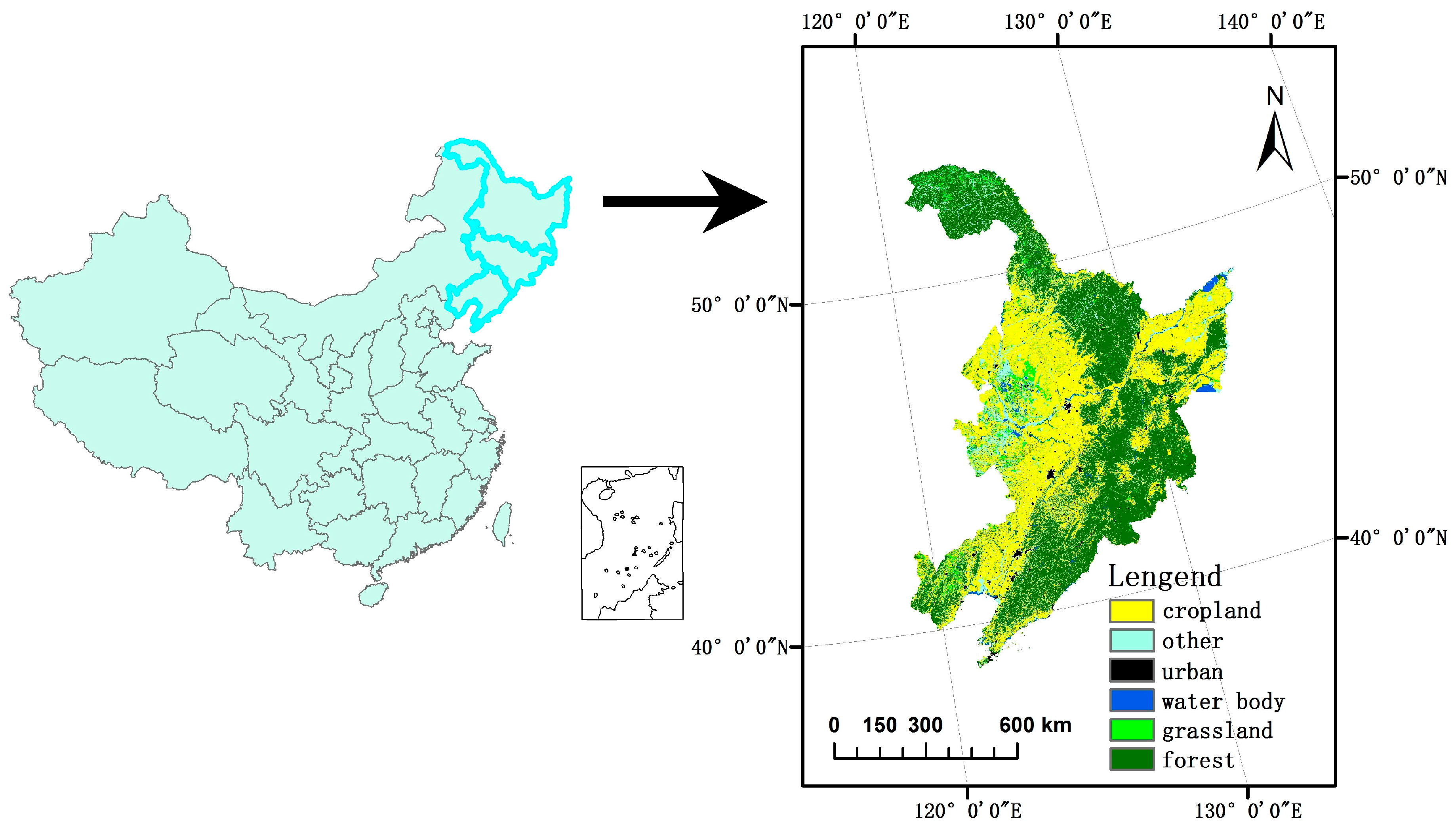
2.1. Study Area

The three provinces, including Heilongjiang, Jilin and Liaoning, are located at 118°50′E–135°09′E, 38°42′N–53°35′N [13] in Northeast China. The total area of the three provinces is about 0.787 million km², accounting for 8.2% of the country’s total area. Most parts of the study area are in the mid-temperate zone, except for the northern part of Heilongjiang province (cold temperate zone) and the southwestern part of Liaoning province (warm temperate zone). The plains with lower altitude primarily situated in the eastern (Songliao Plain) and western (Sanjiang Plain) parts, mountains at a high altitude mainly located in the southeastern (Changbai Mountains) and northern (Lesser Khingan Mountains) parts. The majority of cropland and urban areas are located in Songliao Plain and Sanjiang Plain; the forest area is mainly located in the Lesser Khingan Mountains and the Changbai Mountains (Figure 1). With regard to the population, the total population in Northeast China reached 109.8 million in 2013, and up to 65 million people live in cities [24].

2.2. Land Cover Data

The China’s Land Use/Cover Datasets (CLUDs) were derived from the Landsat Thematic Mapper/Enhanced Thematic Mapper (TM/ETM+) and HJ-1A/1B, including 25 classes in total with 5-year intervals from 1990 to 2015. Quality control procedures have been carried out for the datasets, and the overall accuracy of the 25 classes of CLUDs was up to 90% [25,26,27]. More details about the CLUDs can be found in previous studies [25,26,27,28].

The CLUDs were merged into six major categories (urban, water body, cropland, forest, grassland and other) and resampled to a spatial resolution of 1000 m to match the Moderate-resolution Imaging Spectroradiometer (MODIS) EVI data and MODIS LST data. Then, each category was converted into a vector file for the purpose of subsetting the MODIS EVI data and later statistical analysis. In this study, we hypothesized that the CLUDs in the years 2000, 2005, 2010, and 2015 can represent land use/cover in 2001–2002, 2003–2007, 2008–2012, 2013–2015, respectively [4].

2.3. MODIS EVI Data

This study used the MOD13A2 EVI data (16 days composite, 1000 m spatial resolution, from 2001 to 2015) to extract the LSP information (SOS, EOS and LOS) in Northeast China. This data was improved via de-coupling of canopy background signal and reducing the influences of atmospheric and soil reflectance [29,30]. A lot of studies showed that EVI is better than Normalized Difference Vegetation Index (NDVI), especially for detecting vegetation variations in urban areas [16,31,32,33]. This data was first reprojected and mosaicked using the MODIS Reprojection Tool (MRT) [34]. Then, we removed cropland since the SOS of cropland was affected by artificial sowing, and the EOS of cropland was affected by artificial harvesting. Thus, the cropland cannot accurately reflect the environmental and climate changes. Water body was also removed in this study due to no vegetation covers [9,18,31].

2.4. MODIS LST Data

MODIS LST is ideal data to study the UHI at the regional scale [35,36,37,38], and the absolute bias is less than 1 K [39,40,41]. We used the MOD11A2 LST data (8-day composite, 1000 m spatial resolution, from 2001 to 2015) to detect the temporal variations of UHII in the study area. We used the same method mentioned in the above section to reproject and mosaic the MODIS LST data. We assumed that the mean of MODIS LST nighttime temperature and MODIS LST daytime temperature can represent daily average temperature, the mean temperature during March to May can represent spring temperature, and the mean temperature during September to November can represent autumn temperature, according to a previous study [10].

2.5. Phenology Metrics

TIMESAT was used to generate the LSP information from MODIS EVI data [42,43]. We used the Savitzky–Golay filter to smooth the EVI time series data, according to previous study, since it is simple, reliable and can preserve features of the dataset, such as relative maximum, minimum and width [44]. There are generally two methods to determine the SOS and EOS [4]. The first one is the threshold method, i.e., SOS and EOS were defined as the dates that the fitted curves rise up to and then fall to the threshold value, respectively. The second one is the amplitude method, i.e., SOS and EOS were defined as the date that the fitted curves rise up to and then fall to the proportion of the amplitude, respectively. The amplitude is defined as the differences between the maximal and minimal EVI in the same year. In this study, we chose the amplitude method since urban areas have lower vegetation cover than the surroundings, and the threshold method cannot correctly compute the LSP metrics. Zhao et al. studied the variation of LSP in Northeast China during 1982–2013 [13] using 30% of the amplitude, and the results were in agreement with ground observation and previous studies [45,46,47]. Similarly, we also chose 30% of the amplitude to calculate the LSP parameter (SOS, EOS) for further analysis in this study.

There may be some outliers resulting from atmospheric contamination or interference from human activities when extracting the phenology information. We excluded these outliers for the purpose of reducing the deviation [4]. SOS earlier than day 50 of the year (DOY) or later than 180 DOY was excluded, and EOS earlier than 240 DOY and later than 330 DOY was removed. LOS was computed as the differences between EOS and SOS.

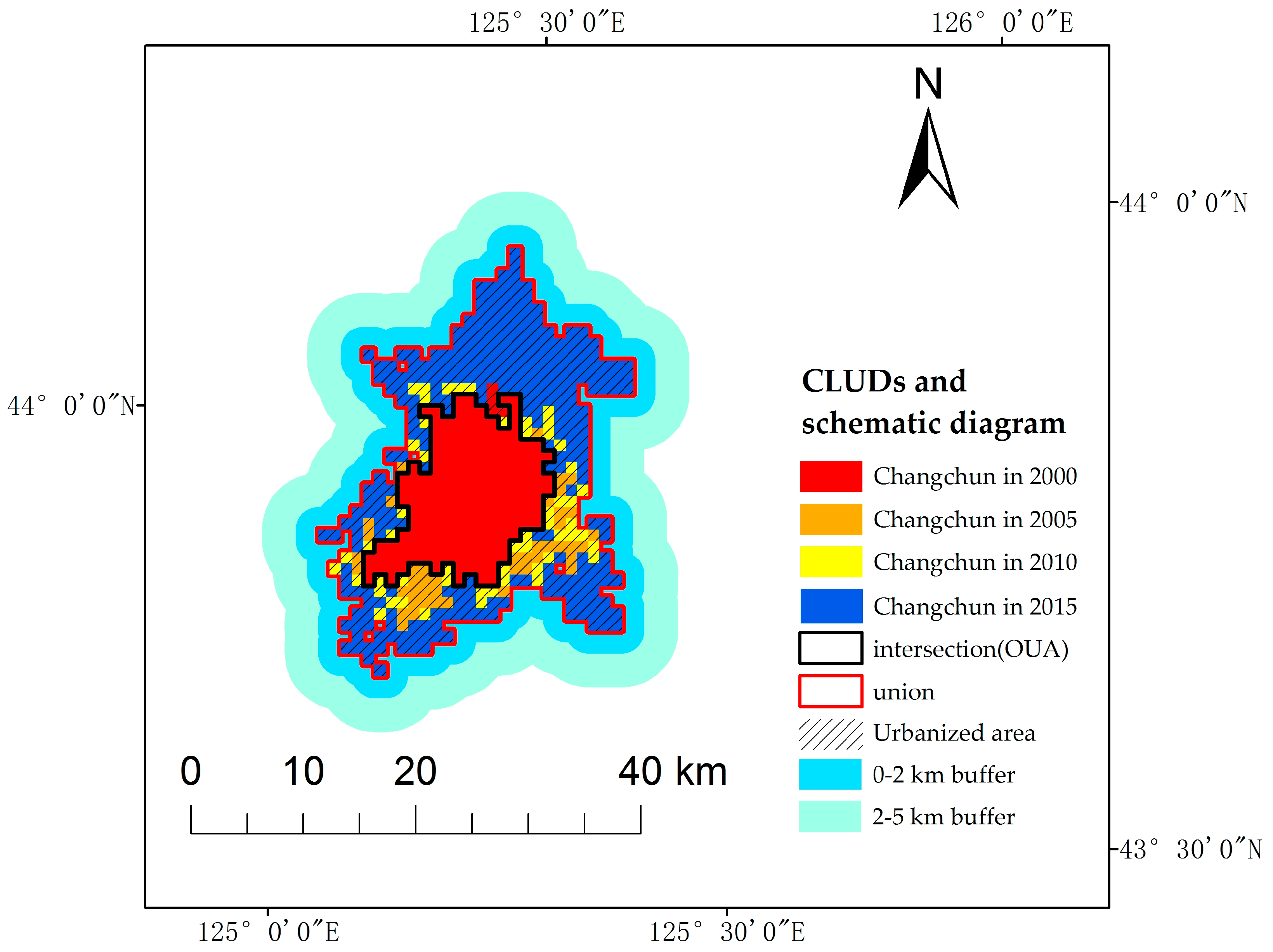
2.6. Calculation of UELSP and UHII

First, we removed the cities with urban areas less than 10 km², since the smaller cities may have slower urbanization speed and smaller UEs [31]. Then, we chose the urban area of the CLUDs (in the years 2000, 2005, 2010, and 2015) to take the intersection and defined it as ”old urban area” (OUA)—that is to say, the OUA was the common part of urban areas over above 4 land cover maps. We take the union of the urban areas of the CLUDs (in the years 2000, 2005, 2010, and 2015), subtract the intersection from the union part, and define it as urbanized area. We further generate 3 buffers extending 0–2 km, 2–5 km, and 20–25 km from the edge of the union and define the 20–25 km buffer as rural area according to [4]. In this way, this study focused on 4 stationary areas in and around the urban area (OUAs, urbanized areas, 0–2 km buffer and 2–5 km buffer) and one stationary area in a rural area (20–25 km buffer) in Northeast China (Figure 2).

We used the phenology differences between OUAs or urbanized areas or buffers (0–2 km buffer, 2–5 km buffer) and rural areas (20–25 km buffer) to represent the UELSP as follows [4]:

$$\Delta \mathrm{P}1={\mathrm{P}}_{\mathrm{OUA}}-{\mathrm{P}}_{\mathrm{rural}}$$

(1)

$$\Delta \mathrm{P}2={\mathrm{P}}_{\mathrm{urbanized}\mathrm{area}}-{\mathrm{P}}_{\mathrm{rural}}$$

(2)

$$\Delta \mathrm{P}3={\mathrm{P}}_{0–2\mathrm{km}\mathrm{buffer}}-{\mathrm{P}}_{\mathrm{rural}}$$

(3)

$$\Delta \mathrm{P}4={\mathrm{P}}_{2–5\mathrm{km}\mathrm{buffer}}-{\mathrm{P}}_{\mathrm{rural}}$$

(4)

where P_OUA, P_{urbanized area}, P_{0-2km buffer}, P_{2-5km buffer} and P_rural represent the LSP metrics (SOS, EOS, LOS) in OUAs, urbanized areas, 0–2 km buffer, 2–5 km buffer and 20–25 km buffer, respectively. Accordingly, ∆P1, ∆P2, ∆P3 and ∆P4 represent the UELSP in OUAs, urbanized areas, 0–2 km buffer and 2–5 km buffer, respectively.

Similarly, we used the LST differences between OUAs or urbanized areas, or buffer zones and rural areas to represent the UHII as follows [4,5,6,7]:

$$\Delta \mathrm{T}1={\mathrm{T}}_{\mathrm{OUA}}-{\mathrm{T}}_{\mathrm{rural}}$$

(5)

$$\Delta \mathrm{T}2={\mathrm{T}}_{\mathrm{urbanized}\mathrm{area}}-{\mathrm{T}}_{\mathrm{rural}}$$

(6)

$$\Delta \mathrm{T}3={\mathrm{T}}_{0–2\mathrm{km}\mathrm{buffer}}-{\mathrm{T}}_{\mathrm{rural}}$$

(7)

$$\Delta \mathrm{T}4={\mathrm{T}}_{2–5\mathrm{km}\mathrm{buffer}}-{\mathrm{T}}_{\mathrm{rural}}$$

(8)

where the T_OUA, T_{urbanized area}, T_{0-2km buffer}, T_{2-5km buffer} and T_rural represent the LST in OUAs, urbanized areas, 0–2 km buffer, 2–5 km buffer and 20–25 km buffer, respectively. Therefore, ∆T1, ∆T2, ∆T3 and ∆T4 represent the UHII in OUAs, urbanized areas, 0–2 km buffer and 2–5 km buffer, respectively.

3. Results

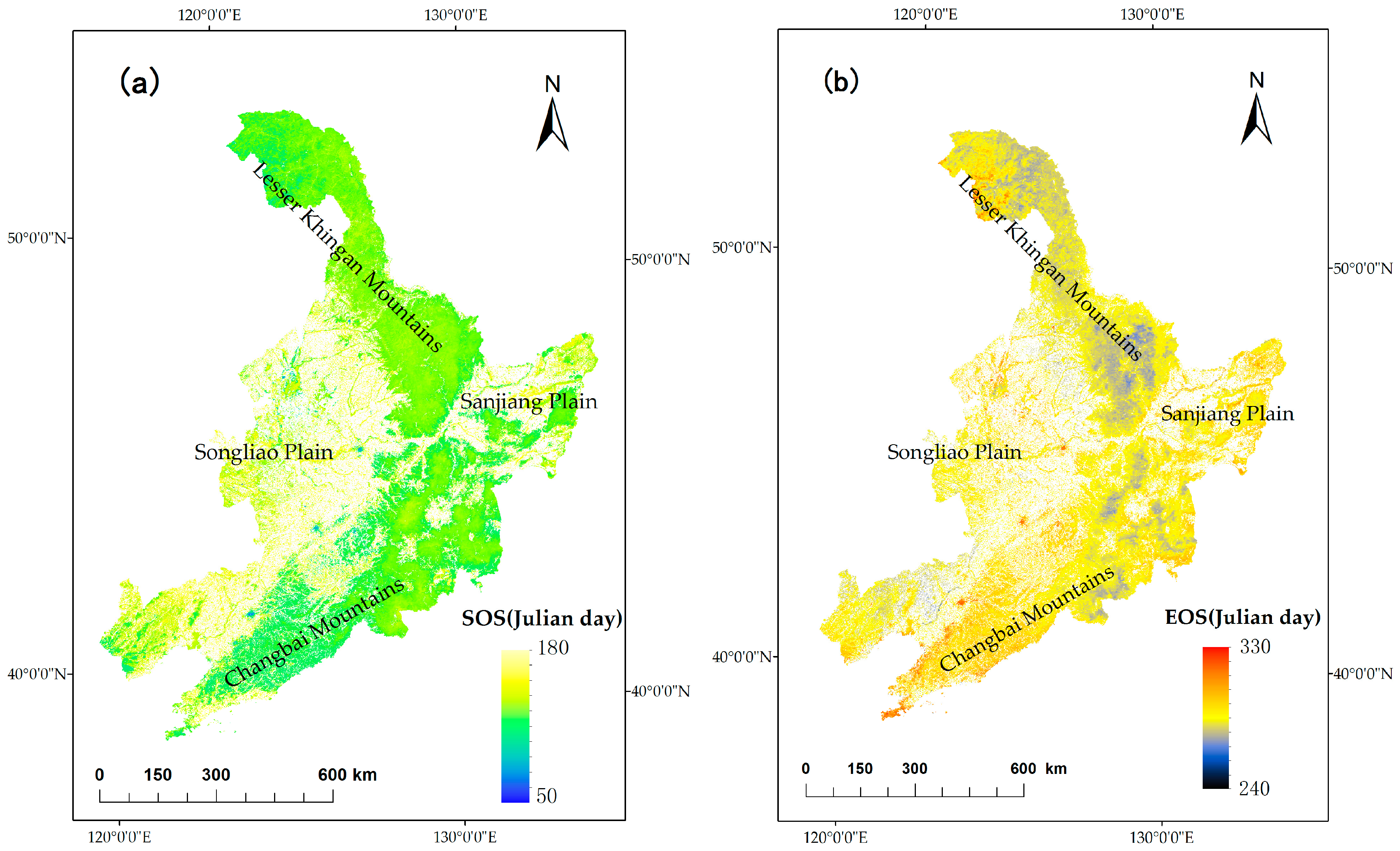
3.1. Mean Phenology and Mean LST in Northeast China

The spatial distributions of annual mean SOS and EOS during 2001–2015 were characterized by high spatial heterogeneity (Figure 3a,b). It was clear that both the earliest SOS and latest EOS were located at the biggest cities such as Harbin, Changchun and Shenyang. The later SOS mainly occurred in Songnen Plain, Liaohe Plain and Sanjiang Plain, and the earlier SOS mostly appeared in the eastern part of Liaoning province. The earlier EOS mainly occurred in the Lesser Khingan Mountains and the northeastern part of the Changbai Mountains, and the later EOS appeared in the southwestern part of the Changbai Mountains.

The mean SOS, EOS, LOS, spring LST, and autumn LST in the four areas (OUAs, urbanized areas, 0–2 km buffer, 2–5 km buffer) during 2001–2015 were shown in

Table 1. The mean SOS, EOS, LOS, spring LST and autumn LST in four areas during 2001–2015.

	SOS(DOY)	EOS(DOY)	LOS(DOY)	Spring LST (°C)	Autumn LST (°C)
Entire study area
OUAs	115.61	305.15	189.54	10.87	10.07
urbanized areas	131.03	298.31	167.28	10.08	9.26
0–2 km buffer	135.41	294.23	158.82	9.21	8.48
2–5 km buffer	136.68	291.48	154.8	8.81	7.88
20–25 km buffer	132.41	289.19	156.78	7.99	7.28
Heilongjiang province
OUAs	115.66	304.35	188.69	8.38	6.91
urbanized area	133.21	296.30	163.09	7.62	6.25
0–2 km buffer	139.11	292.46	153.35	6.81	5.65
2–5 km buffer	139.43	290.52	151.09	6.28	5.28
20–25 km buffer	133.25	287.06	153.81	5.59	4.9
Jilin province
OUAs	114.01	304.5	190.49	10.04	9.03
urbanized areas	130.40	297.00	166.6	9.22	8.18
0–2 km buffer	135.67	291.54	155.87	8.68	7.61
2–5 km buffer	137.15	289.28	152.13	8.45	7.30
20–25 km buffer	132.73	289.3	156.57	8.02	7.26
Liaoning province
OUAs	116.18	305.88	189.7	12.87	12.75
urbanized areas	129.3	300.14	170.84	12.11	11.87
0–2 km buffer	133.72	296.32	162.6	11.49	11.05
2–5 km buffer	134.9	293.49	158.59	11.18	10.59
20–25 km buffer	131.31	291.07	159.76	11.01	10.44

SOS is short for start of the growing season, EOS: end of the growing season, LOS: length of the growing season, LST: spring land surface temperature, DOY: day of year; OUAs: old urban areas.

, where the strongest UHII and UELSP were found in OUAs. The mean spring LST, autumn LST and EOS decreased with the increasing distances from OUAs. SOS first increased then decreased, but LOS first decreased and then rose with increasing distances from OUAs.

In addition, the LST increases with increasing latitude, the warmest province is Liaoning and the coldest province is Heilongjiang. Meanwhile, in rural areas (20–25 km buffer), the earliest SOS and the latest EOS is in Liaoning province, the latest SOS and the earliest EOS are in Heilongjiang province, but the LSP differences between different provinces is not evident.

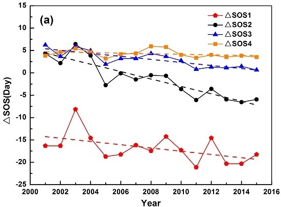
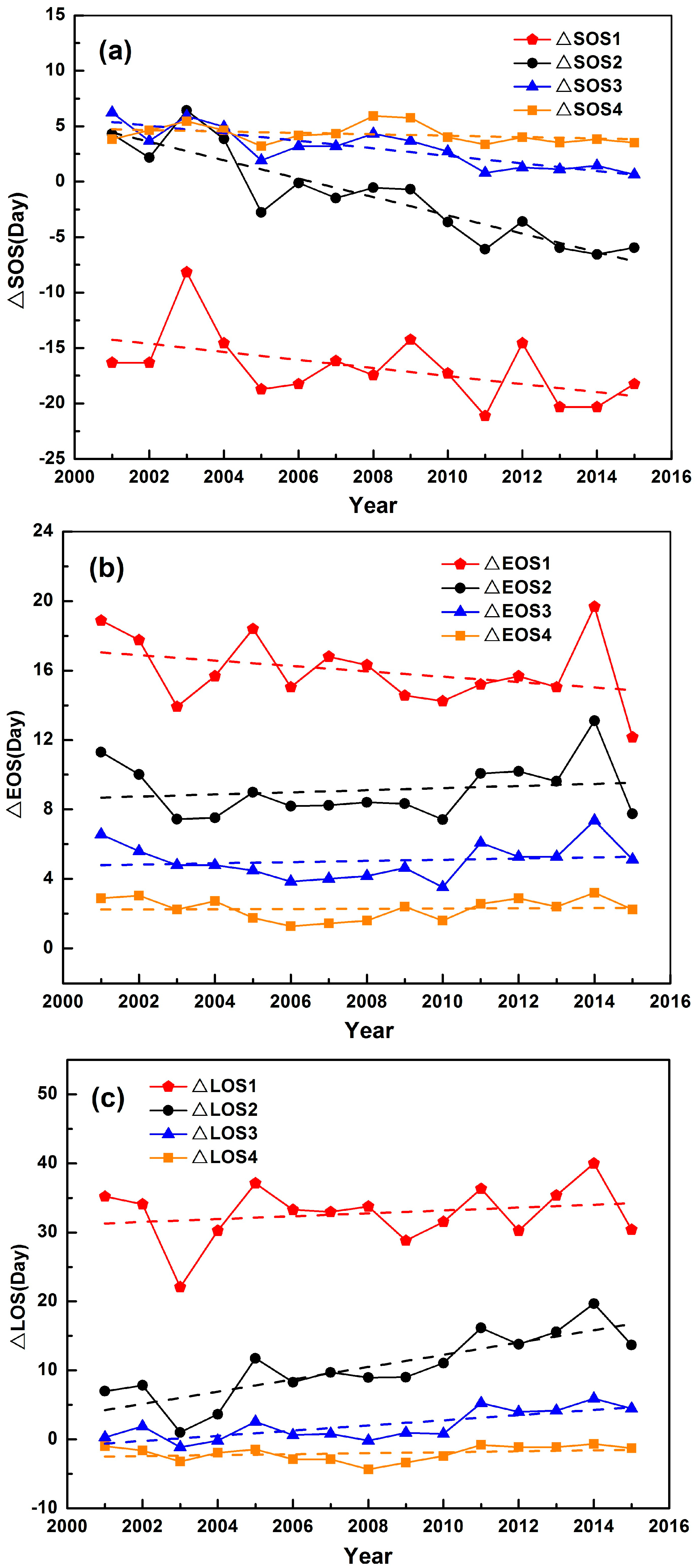
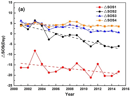
3.2. Temporal Variations of UELSP

This study analyzed the temporal variations of UELSP in four areas in Northeast China during 2001–2015. The ∆SOS decreased in four areas (Figure 4a). The UEs on SOS was evident in OUAs (Table 1), and there was a significant decreasing trend (−0.30 days/year) during 2001–2015. The ∆SOS decreased significantly in urbanized area (−0.79 days/year, p < 0.01) and 0–2 km buffer (−0.35 days/year, p < 0.01). Meanwhile, the ∆SOS decreased in 2–5 km buffer (−0.07 days/year). The results from the above analysis suggested that the SOS in OUAs had become earlier and earlier compared to rural areas, and the differences in SOS between urbanized areas and rural areas changed greatly during 2001–2015.

On the contrary, ∆EOS was always greater than zero in the four areas during 2001–2015, which suggested that the urbanization can postpone the EOS in and around the urban area. However, the results of ∆EOS did not increase or decrease significantly in all of the four areas above (Figure 4b): OUAs (−0.24 days/year), urbanized areas (0.05 days/year), 0–2 km buffer (0.03 days/year), and 2–5 km buffer (0.00 days/year). It suggested that the UEs on EOS did not change during the whole study period in Northeast China.

It can be seen from Figure 4c that the ∆LOS increased in four areas during 2001–2015. The mean LOS in OUAs was 32.76 days longer than that in rural areas (Table 1), and the differences between the OUAs and rural areas increased at the rate of 0.05 days/year. The ∆LOS increased significantly in urbanized areas (0.92 days/year, p < 0.01) and 0–2 km buffer (0.35 days/year, p < 0.01), but ∆LOS only increased at the rate of 0.05 days/year in a 2–5 km buffer, which was much lower than those in urbanized areas and the 0–2 km buffer. These results indicated that the LOS in urban and surrounding areas became increasingly longer than that in rural areas. Overall, the areas that had the most significant changes of UEs on SOS and LOS during 2001–2015 were urbanized areas, followed by the 0–2 km buffer and OUAs in Northeast China.

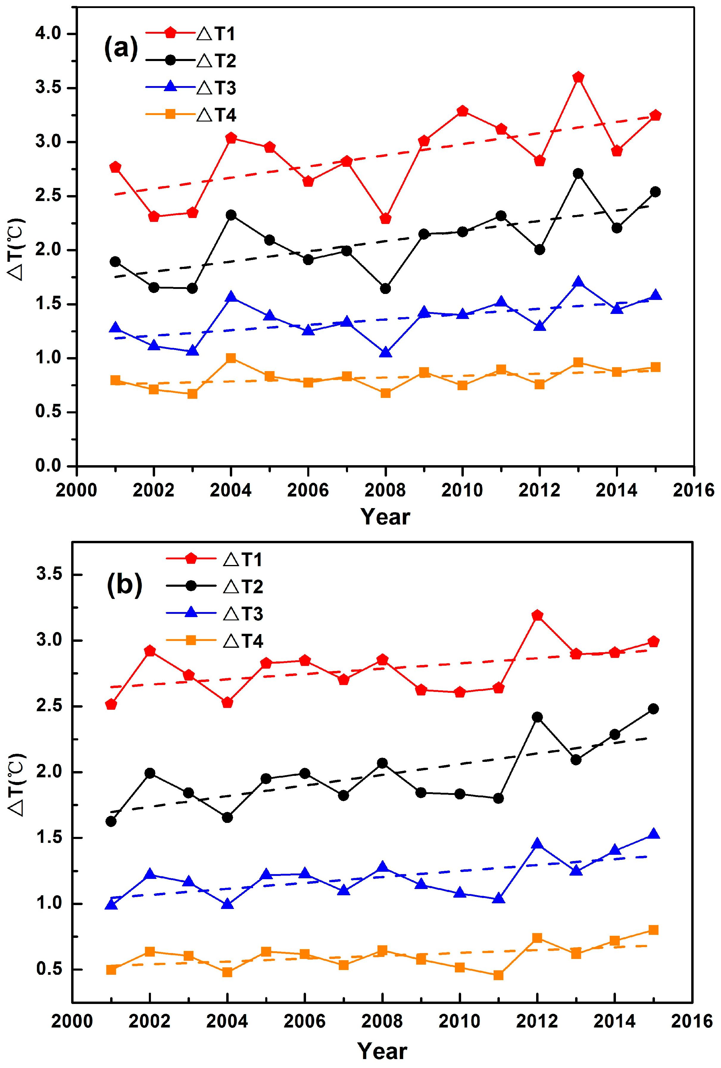
3.3. Temporal Variations of UHII

The interannual variations of UHII in Northeast China were also analyzed in this study. As shown in Figure 5a, the UHII in spring increased significantly in OUAs (0.052 °C/year, p < 0.05), urbanized areas (0.050 °C/year, p < 0.05), 0–2 km buffer (0.025 °C/year, p < 0.05) but insignificantly in a 2–5 km buffer (0.010 °C/year). It is worth noting that the stronger the UHII, the larger the increasing trends of UHII during 2001–2015. Meanwhile, the UHII in autumn also increased in the four areas during 2001–2015 (Figure 5b). The ∆T for urbanized areas increased at the rate of 0.038 °C/year (p < 0.05), which was higher than that at the 0–2 km buffer (0.022 °C/year, p < 0.05), OUAs (0.016 °C/year) and 2–5 km buffer (0.011 °C/year).

Overall, the ∆T in spring and autumn were always greater than zero in all four of the areas (in the spring of 2013, the UHII even reached 3.5 °C for OUAs), which suggested that the intensity of UHI was evident in Northeast China, and the footprint of UHI not only included the urban areas but also the suburbs during the study period. The most important point is that the UHII increased in both spring and autumn in four areas during 2001–2015, and the temporal variations of UHII in spring and autumn are all highly significant in urbanized areas, indicating that the rapid urbanization and land use/cover change led to the intensification of UHI in Northeast China.

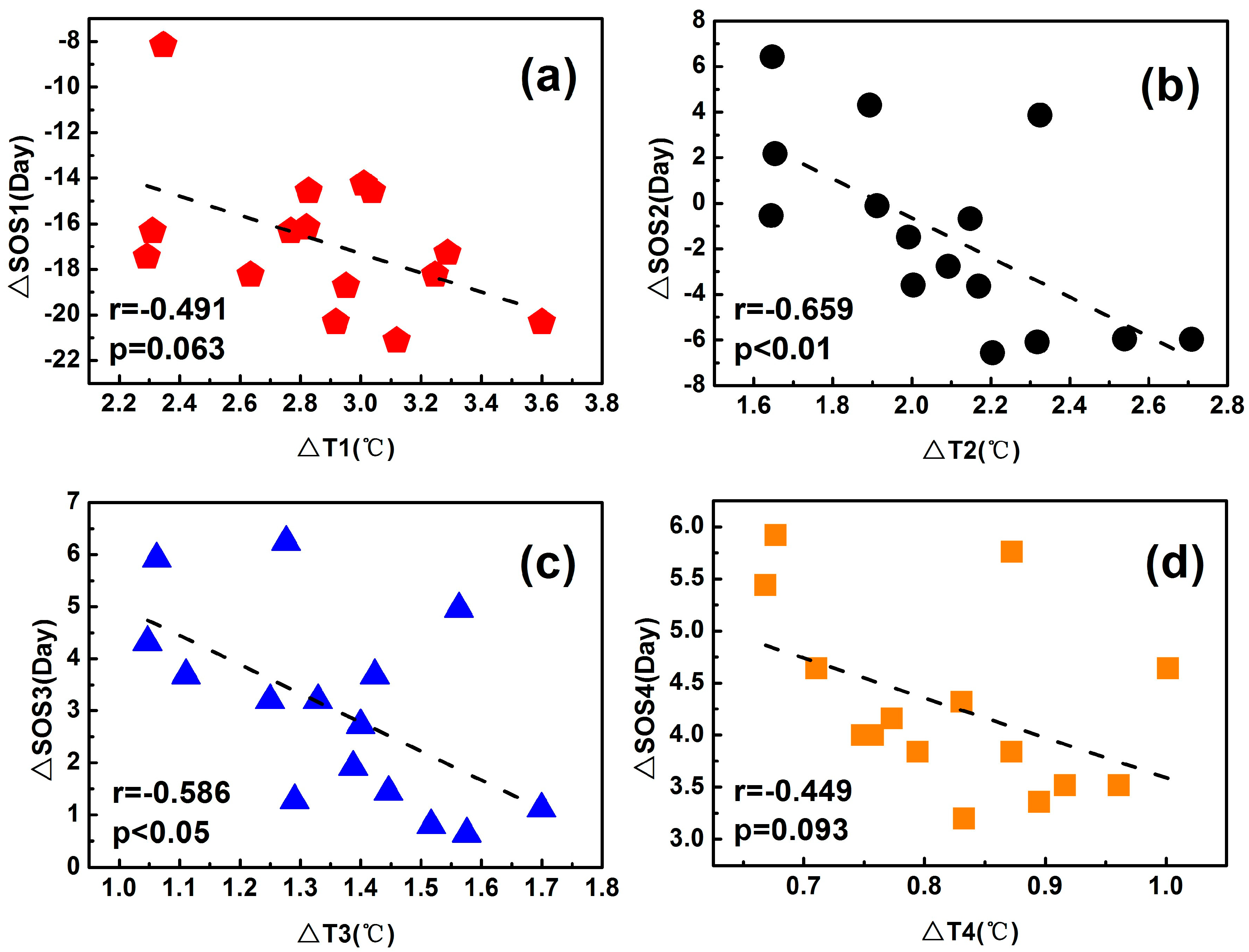
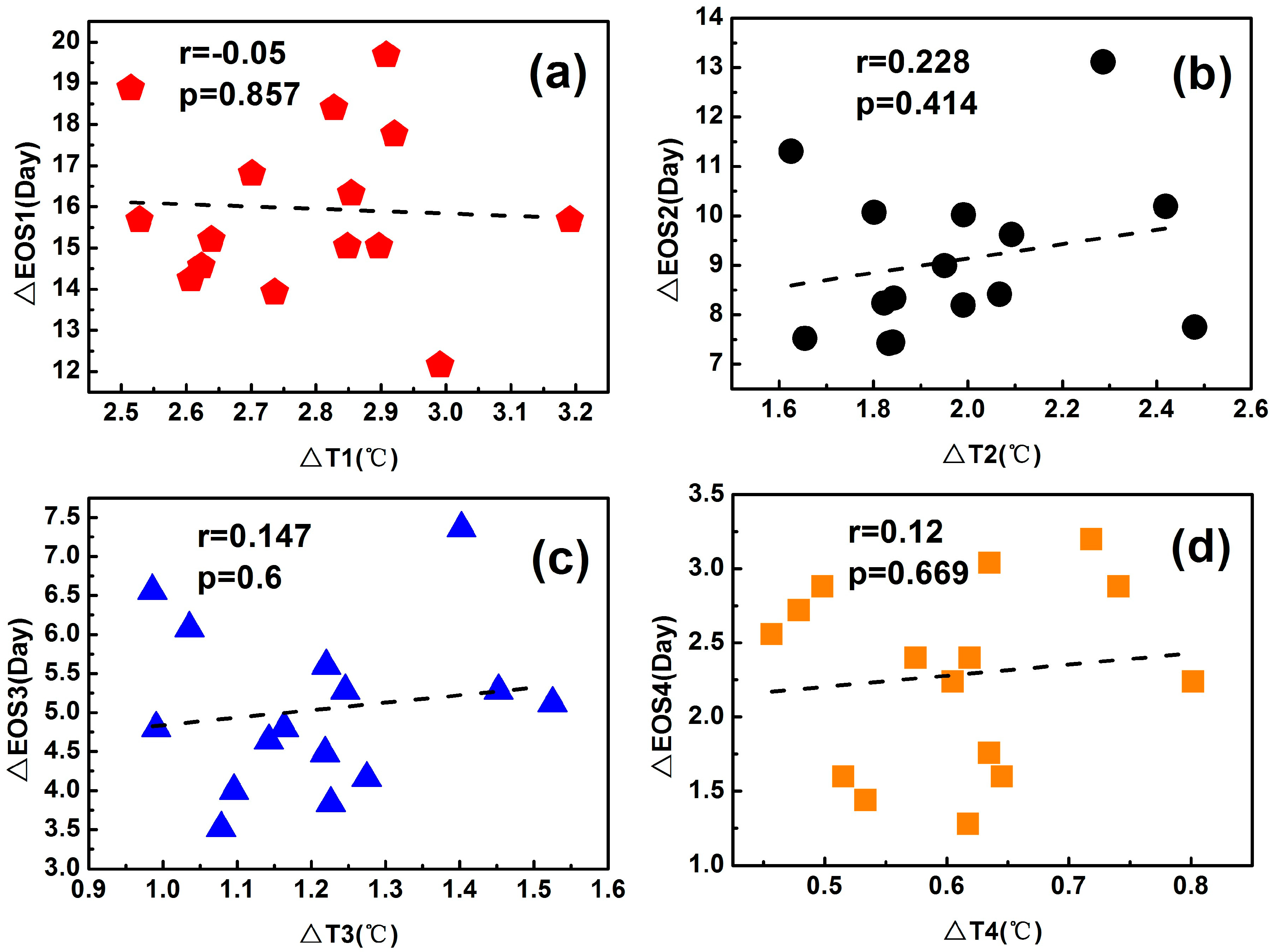
3.4. Correlations between UHII and UELSP

The correlation analysis between ∆T and ∆P were conducted to investigate the relationships between the UELSP and UHII in this study. It was clear from Figure 6 that the correlations between ∆SOS and ∆T in spring were all negative in four areas: OUAs (Figure 6a; r = −0.491, p = 0.063), urbanized areas (Figure 6b; r = −0.659, p < 0.01), 0–2 km buffer (Figure 6c; r = −0.586, p < 0.05) and 2–5 km buffer (Figure 6d; r = −0.449, p = 0.093). There were significant correlations between ∆T and ∆SOS in urbanized areas (p < 0.01) and 0–2 km buffer (p < 0.05), indicating that the SOS became earlier and earlier with increasing UHII in spring in four areas compared to that in rural areas (20–25 km).

However, there were almost no significant correlations between UHII and the UEs on EOS in autumn for the four areas above: OUAs (Figure 7a; r = −0.05, p = 0.857), urbanized areas (Figure 7b; r = 0.228, p = 0.414), 0–2 km buffer (Figure 7c; r = 0.147, p = 0.6) and 2–5 km buffer (Figure 7d; r = 0.12, p = 0.669). The correlation coefficients between ∆EOS and ∆T in autumn in the four areas only ranged between −0.05 and 0.228, indicating that the increasing UHII in autumn did not contribute to the increasing UEs on EOS in Northeast China.

4. Discussion

4.1. Mean UHII and LSP

We calculated the 15-year averaged phenology metrics (SOS, EOS) in the whole study area and in the forest area, respectively. In general, the spatial distributions of mean SOS and EOS during 2001–2015 in this study were similar to that of Zhao et al., where the glaobal inventory modelling and mapping studies (IMMS) NDVI3g data were used to study the variations of LSP in Northeast China during 1982–2013 [13]. Their results showed that SOS in the plain areas was later than in the mountains, and EOS in the southern areas were later than that in the north. In addition, the average SOS for the whole study area during 2001–2015 in our study was mainly between 112 and 161 DOY, the average SOS of the forest area was primarily between 113 and 151 DOY, EOS was mainly between 273 and 300 DOY, and the EOS in the forest area was primarily between 273 and 299 DOY. These results were also in line with previous studies [13,45,46,47] (

Table 2. Mean land surface phenology (LSP) compared with other studies.

	This Study	Zhao et al. [14]	Yu et al. [44]	Hou et al. [45]	Yu et al. [46]
SOS of entire study area (Jlian day)	112–161	110–150
EOS of entire study area (Jlian day)	273–300	270–320
SOS of forest (Jlian day)	113–151		100–150	110–140	100–140
EOS of forest (Jlian day)	273–299		260–290	260–290	265–300
Time period (year)	2001–2015	1982–2013	2003	2001–2010	2000–2009

), which suggested that the method of extraction of the phenology metrics in this study was reliable.

Moreover, it was revealed in this study that the UELSP and UHII were evident in OUAs, and the average differences of SOS, EOS and LOS between OUAs and rural areas were −16.8 days, 15.96 days and 32.76 days, respectively, during the last 15 years. These effects were close to the study [4] and much larger than some previous studies [16,18,19], which is probably due to the different species compositions (deciduous forest vs. evergreen forest) and geographic locations. Specifically, northeast China was mainly covered by deciduous forest, but some cities (e.g., tropical cities of China) were primarily covered by evergreen vegetation in literature [9], which can lead to the differences in seasonal variations of the vegetation index and the differences of UELSP. The 15-year averaged UHII in spring and autumn in OUAs were 2.88 °C and 2.79 °C (Table 1), respectively. These results were higher than previous studies [5,48]. The reason may be due to the different definitions for rural areas, Zhou et al. showed that the footprint of UHI in China was 2.3 and 3.9 times the urban areas for day and night, respectively [4]. Accordingly, ignoring the footprint of UHI can lead to underestimating the UHII. In this study, the rural area (20–25 km buffer) that we chose was farther from the urban area compared to previous studies [5,48], and it is far away from the UEs [9]. Thus, the method in this study may provide a more accurate assessment of the UELSP and UHII. In addition, the trends of LSP and LST, along with the urban-rural gradient, were similar to studies from Han et al., which studied the LSP and LST in six cities in the Yangtze River Delta, China [16]. Their results showed that LST decreased with the increasing distances from urban areas, and EOS decreased with increasing distances from urban areas, but SOS increased first and then decreased along the urban-rural gradient.

4.2. Temporal Variations of UHII and UELSP in Addition to Possible Reasons

The UELSP may change greatly due to rapid urbanization, so this study highlighted the temporal variations of UELSP and UHII. The UHII in spring and autumn has experienced dramatic changes in OUAs, urbanized areas and 0–2 km buffer during 2001–2015 in Northeast China (Figure 5), and the UEs on SOS and LOS has significant temporal variations in urbanized areas and 0–2 km buffer (Figure 3). It is worth noting that the largest changes of UEs on SOS, LOS, and UHII in autumn are in urbanized areas, and the temporal variations of UHII in spring, UHII in autumn, and UEs on SOS and LOS in urbanized areas are all highly significant (

Table 3. Linear trends of ∆SOS, ∆EOS, ∆LOS, ∆T in spring and ∆T in autumn in four regions (OUAs, urbanized areas, 0–2 km buffer, 2–5 km buffer).

	∆SOS	∆EOS	∆LOS	∆T in Spring	∆T in Autumn
OUAs	−0.363	−0.155	0.208	0.052 *	0.02
urbanized areas	−0.829 **	0.061	0.89 **	0.047 **	0.04 **
0–2 km buffer	−0.34 **	0.034	0.374 **	0.025 *	0.023 *
2–5 km buffer	−0.063	0.007	0.07	0.009	0.011

Significance levels: * p < 0.05; ** p < 0.01.

). This might be attributed to the land use/land cover change. With rapid urbanization, other land cover types may transform into urban areas, such as cropland and forest. Therefore, more environmental changes may occur in urbanized areas, such as lower vegetation coverage, higher impervious surface, and denser population. The main factors influenced the increases of UHII may be the lower vegetation cover and higher impervious surface in the study area. On one hand, vegetation can reduce the LST to some extent, which has been confirmed by some studies in literature [49,50,51,52,53,54,55]: increasing vegetation cover was regarded as an effective way to reduce the UHII, since vegetation can release latent heat flux by evapotranspiration. On the other hand, studies have showed that impervious surface has significant positive correlation with LST [49,56]. Impervious surface can increase the UHII, since it can absorb and store heat during the daytime and release slowly during the nighttime. Therefore, the UELSP may increase with increasing UHII in urban areas. In addition, other factors such as species compositions resulted from land cover changes that may also have direct effects on LSP [9].

4.3. Relationships between UHII and UELSP

In this study, there were large correlations between UHII and the UEs on SOS in spring in four areas: OUAs (r = −0.491, p = 0.063), urbanized areas (r = −0.659, p < 0.01), 0–2 km buffer (r = −0.586, p < 0.05) and 2–5 km buffer (r = −0.449, p = 0.093) during 2001–2015. The results suggested that the great changes of UEs on SOS were mainly attributed to the increasing UHII in spring. However, there were almost no significant correlations between UHII and the UEs on EOS in autumn. Although the UHII increased in autumn, the impacts of urbanization on EOS did not change significantly. This phenomenon is similar to previous studies [9,31], and Zhang et al. showed that there was a significant linear relationship between ∆SOS and ∆LST during January to May, but the relationship between ∆EOS and ∆LST during September to December was not significant in eastern North America [31]. Zhou et al. also showed that the cities with earlier SOS were obviously more than the cities with later EOS in China [9]. The reason for this phenomenon may be that the EOS was also affected by other important factors such as water and photoperiod [31]. Previous studies also showed that earlier SOS may trigger earlier EOS because vegetation may reach the carbohydrate storage capacity with earlier SOS and then lead to earlier EOS [15]. In addition, Northeast China is located at high latitudes, sunshine duration may play an important role in influencing LSP (for example, the advanced SOS and delayed EOS) [14]. Overall, EOS has complex correlations with SOS, temperature, precipitation, sunshine duration and some other factors, and more detailed studies needed to be carried out in future studies.

4.4. Uncertainty

There were still some uncertainties for analyzing the UELSP in Northeast China in this study. Firstly, we used the CLUDs in the years 2000, 2005, 2010, and 2015, which represented those in 2001–2002, 2003–2007, 2008–2012, and 2013–2015, respectively. This may lead to some uncertainties in urban areas, especially in fast-growing cities. In addition, a lot of other factors may influence the LSP and the phenology results such as species compositions, interference from human activities, and altitudes. Finally, the reasons that the increasing UHII in autumn did not lead to increases of UEs on EOS were still not clear. The comprehensive analysis between EOS, SOS, temperature, precipitation, sunshine duration and other factors should be conducted in detail in future studies.

5. Conclusions

In this study, MODIS LST, MODIS EVI and CLUDs were used to analyze the UHII and UELSP and the associated temporal variations in Northeast China during 2001–2015. The UHII and UELSP were investigated by studying the LST and LSP differences between urban and rural areas, respectively. Correlation analysis was also conducted to reveal the relationships between UHII and UELSP.

The results showed that the UELSP was evident in Northeast China, especially in big cities such as Harbin, Changchun and Shenyang. The annual mean UHII in OUAs is 2.88 °C in spring and 2.79 °C in autumn during the whole study period. The differences of annual mean LSP between OUAs and rural areas were −16.8 days for SOS, 15.96 days for EOS and 32.76 days for LOS, respectively. The SOS in the four areas above has become earlier and earlier compared to rural areas, especially in urbanized areas (−0.79 days/year, p < 0.01) during 2001–2015, and the LOS in the four areas above has become longer and longer compared to rural areas, especially in urbanized areas (0.92 days/year, p < 0.01), but the UEs on EOS (∆EOS) did not change significantly during the whole study period. Meanwhile, the UHII in spring and autumn months increased in four areas, especially in OUAs (0.052 °C/year, p < 0.05 in spring, and 0.016 °C/year in autumn), urbanized areas (0.050 °C/year, p < 0.05 in spring, and 0.038 °C/year, p < 0.05 in autumn), 0–2 km buffer (0.025 °C/year, p < 0.05 in spring, and 0.022 °C/year, p < 0.05 in autumn). Finally, the correlation analysis indicated that the increasing UHII in spring contributed greatly to the changes of UEs on SOS, but the increasing UHII in autumn did not lead to changes of UEs on EOS in Northeast China.

Overall, this study provided an important reference for investigating the spatial-temporal trends of UHII and UEs on the terrestrial ecosystem, but there were still some uncertainties in our research, and the correlation between EOS and its influencing factors need to be investigated thoroughly in later studies.

References

1. Mimet, A.; Pellissier, V.; Quénol, H.; Aguejdad, R.; Dubreuil, V.; Rozé, F. Urbanisation induces early flowering: evidence from Platanus acerifolia and Prunus cerasus. Int. J. Biometeorol. 2009, 53, 287–298. [Google Scholar] [CrossRef] [PubMed]
2. United Nation Population Division. Available online: https://esa.un.org/unpd/wup/DataQuery/ (accessed on 30 October 2016).
3. Krehbiel, C.P.; Jackson, T.; Henebry, G.M. Web-Enabled Landsat data time series for monitoring urban heat island impacts on land surface phenology. IEEE J. Sel. Top. Appl. Earth Obs. Remote Sens. 2016, 9, 2043–2050. [Google Scholar] [CrossRef]
4. Zhou, D.; Zhao, S.; Zhang, L.; Liu, S. Remotely sensed assessment of urbanization effects on vegetation phenology in China’s 32 major cities. Remote Sens. Environ. 2016, 176, 272–281. [Google Scholar] [CrossRef]
5. Zhou, D.; Zhao, S.; Zhang, L.; Sun, G.; Liu, Y. The footprint of urban heat island effect in China. Sci. Rep. 2015, 5, 11160. [Google Scholar] [CrossRef] [PubMed]
6. Peng, S.; Piao, S.; Ciais, P.; Friedlingstein, P.; Ottle, C.; Bréon, F.; Nan, H.; Zhou, L.; Myneni, R.B. Surface urban heat island across 419 global big cities. Environ. Sci. Technol. 2012, 46, 696–703. [Google Scholar] [CrossRef]
7. Zhou, D.; Zhao, S.; Liu, S.; Zhang, L.; Zhu, C. Surface urban heat island in China’s 32 major cities: Spatial patterns and drivers. Remote Sens. Environ. 2014, 152, 51–61. [Google Scholar] [CrossRef]
8. Clinton, N.; Gong, P. MODIS detected surface urban heat islands and sinks: Global locations and controls. Remote Sens. Environ. 2013, 134, 294–304. [Google Scholar] [CrossRef]
9. Arnfield, A.J. Two decades of urban climate research: a review of turbulence, exchanges of energy and water, and the urban heat island. Int. J. Climatol. 2003, 23, 1–26. [Google Scholar] [CrossRef]
10. Kang, X.; Hao, Y.; Cui, X.; Chen, H.; Huang, S.; Du, Y.; Li, W.; Kardol, P.; Xiao, X.; Cui, L. Variability and changes in climate, phenology, and gross primary production of an Alpine wetland ecosystem. Remote Sens. 2016, 8, 391. [Google Scholar] [CrossRef]
11. Cecchi, L.; d’Amato, G.; Ayres, J.; Galan, C.; Forastiere, F.; Forsberg, B.; Gerritsen, J.; Nunes, C.; Behrendt, H.; Akdis, C. Projections of the effects of climate change on allergic asthma: The contribution of aerobiology. Allergy 2010, 65, 1073–1081. [Google Scholar] [CrossRef] [PubMed]
12. Van Vliet, A.J.; Overeem, A.; de Groot, R.S.; Jacobs, A.F.; Spieksma, F. The influence of temperature and climate change on the timing of pollen release in the Netherlands. Int. J. Climatol. 2002, 22, 1757–1767. [Google Scholar] [CrossRef]
13. Zhao, J.; Wang, Y.; Zhang, Z.; Zhang, H.; Guo, X.; Yu, S.; Du, W.; Huang, F. The variations of land surface phenology in Northeast China and its responses to climate change from 1982 to 2013. Remote Sens. 2016, 8, 400. [Google Scholar] [CrossRef]
14. Liang, S.; Shi, P.; Li, H. Urban spring phenology in the middle temperate zone of China: Dynamics and influence factors. Int. J. Biometeorol. 2016, 60, 531–544. [Google Scholar] [CrossRef] [PubMed]
15. Wu, C.; Hou, X.; Peng, D.; Gonsamo, A.; Xu, S. Land surface phenology of China’s temperate ecosystems over1999–2013: Spatial–temporal patterns, interaction effects, covariation with climate and implications for productivity. Agric. For. Meteorol. 2016, 216, 177–187. [Google Scholar] [CrossRef]
16. Han, G.; Xu, J. Land surface phenology and land surface temperature changes along an urban–rural gradient in Yangtze River Delta, China. Environ. Manag. 2013, 52, 234–249. [Google Scholar] [CrossRef]
17. Buyantuyev, A.; Wu, J. Urbanization diversifies land surface phenology in arid environments: Interactions among vegetation, climatic variation, and land use pattern in the Phoenix metropolitan region, USA. Landsc. Urban Plan. 2012, 105, 149–159. [Google Scholar] [CrossRef]
18. White, M.A.; Nemani, R.R.; Thornton, P.E.; Running, S.W. Satellite evidence of phenological differences between urbanized and rural areas of the eastern United States deciduous broadleaf forest. Ecosystems 2002, 5, 260–277. [Google Scholar] [CrossRef]
19. Dallimer, M.; Tang, Z.; Gaston, K.J.; Davies, Z.G. The extent of shifts in LSP between rural and urban areas within a human-dominated region. Ecol. Evol. 2016, 6, 1942–1953. [Google Scholar] [CrossRef] [PubMed]
20. Jochner, S.C.; Sparks, T.H.; Estrella, N.; Menzel, A. The influence of altitude and urbanization trends and mean dates in phenology (1980–2009). Int. J. Biometeorol. 2012, 56, 387–394. [Google Scholar] [CrossRef] [PubMed]
21. Gazal, R.; White, M.A.; Gillies, R.; Rodemaker, E.; Sparrow, E.; Gordon, L. GLOBE students, teachers, and scientists demonstrate variable differences between urban and rural leaf phenology. Glob. Chang. Biol. 2008, 14, 1568–1580. [Google Scholar] [CrossRef]
22. Neil, K.; Wu, J. Effects of urbanization on plant flowering phenology: A review. Urban Ecosyst. 2006, 9, 243–257. [Google Scholar] [CrossRef]
23. Luo, Z.; Sun, O.J.; Ge, Q.; Xu, W.; Zheng, J. Phenological responses of plants to climate change in an urban environment. Ecol. Res. 2007, 22, 507–514. [Google Scholar] [CrossRef]
24. Liu, S.; Zhang, P.; Wang, Z.; Liu, W.; Tan, J. Measuring the sustainable urbanization potential of cities in Northeast China. J. Geogr. Sci. 2016, 26, 549–567. [Google Scholar] [CrossRef]
25. Liu, J.; Kuang, W.; Zhang, Z.; Xu, X.; Qin, Y.; Ning, J.; Zhou, W.; Zhang, S.; Li, R.; Yan, C.; et al. Spatiotemporal characteristics, patterns, and causes of land-use changes in China since the late 1980s. J. Geogr. Sci. 2014, 24, 195–210. [Google Scholar] [CrossRef]
26. Liu, J.; Zhang, Z.; Xu, X.; Kuang, W.; Zhou, W.; Zhang, S.; Li, R.; Yan, C.; Yu, D.; Wu, S.; Jiang, N. Spatial patterns and driving forces of land use change in China during the early 21st century. J. Geogr. Sci. 2010, 20, 483–494. [Google Scholar] [CrossRef]
27. Liu, J.; Liu, M.; Zhuang, D.; Zhang, Z.; Deng, X. Study on spatial pattern of land-use change in China during 1995–2000. Sci. China Ser. D 2003, 46, 373–384. [Google Scholar]
28. Kuang, W.; Liu, J.; Dong, J.; Chi, W.; Zhang, C. The rapid and massive urban and industrial land expansions in China between 1990 and 2010: A CLUD-based analysis of their trajectories, patterns, and drivers. Landsc. Urban Plan. 2016, 145, 21–33. [Google Scholar] [CrossRef]
29. Huete, A.; Didan, K.; Miura, T.; Rodriguez, E.P.; Gao, X.; Ferreira, L.G. Overview of the radiometric and biophysical performance of the MODIS vegetation indices. Remote Sens. Environ. 2002, 83, 195–213. [Google Scholar] [CrossRef]
30. Ishtiaque, A.; Myint, S.W.; Wang, C. Examining the ecosystem health and sustainability of the world’s largest mangrove forest using multi-temporal MODIS products. Sci. Total Environ. 2016, 569, 1241–1254. [Google Scholar] [CrossRef] [PubMed]
31. Zhang, X.; Friedl, M.A.; Schaaf, C.B.; Strahler, A.H.; Schneider, A. The footprint of urban climates on vegetation phenology. Geophys. Res. Lett. 2004, 31. [Google Scholar] [CrossRef]
32. Dallimer, M.; Tang, Z.; Bibby, P.R.; Brindley, P.; Gaston, K.J.; Davies, Z.G. Temporal changes in green space in a highly urbanized region. Biol. Lett. 2011, 7, 763–766. [Google Scholar] [CrossRef] [PubMed]
33. Zhou, D.; Zhao, S.; Liu, S.; Zhang, L. Spatiotemporal trends of terrestrial vegetation activity along the urban development intensity gradient in China’s 32 major cities. Sci. Total Environ. 2014, 488, 136–145. [Google Scholar] [CrossRef] [PubMed]
34. LPDAAC (Land Processes Distributed Active Archive Center). MODIS Reprojection Tool. Available online: https://lpdaac.usgs.gov/tools/modis_reprojection_tool (accessed on 7 July 2014).
35. Qiao, Z.; Tian, G.; Xiao, L. Diurnal and seasonal impacts of urbanization on the urban thermal environment: A case study of Beijing using MODIS data. ISPRS. J. Photogramm. 2013, 85, 93–101. [Google Scholar] [CrossRef]
36. Jin, M.; Dickinson, R.E.; Zhang, D. The footprint of urban areas on global climate as characterized by MODIS. J. Clim. 2005, 18, 1551–1565. [Google Scholar] [CrossRef]
37. Hung, T.; Uchihama, D.; Ochi, S.; Yasuoka, Y. Assessment with satellite data of the urban heat island effects in Asian mega cities. Int. J. Appl. Earth. Obs. 2006, 8, 34–48. [Google Scholar]
38. Pongracz, R.; Bartholy, J.; Dezso, Z. Remotely sensed thermal information applied to urban climate analysis. Adv. Space Res. 2006, 37, 2191–2196. [Google Scholar] [CrossRef]
39. Wan, Z. New refinements and validation of the MODIS land-surface temperature/emissivity products. Remote Sens. Environ. 2008, 112, 59–74. [Google Scholar] [CrossRef]
40. Pablos, M.; Martínez-Fernández, J.; Piles, M.; Sánchez, N.; Vall-llossera, M.; Camps, A. Multi-temporal evaluation of soil moisture and land surface temperature dynamics using in situ and satellite observations. Remote Sens. 2016, 8, 587. [Google Scholar] [CrossRef]
41. Gow, L.J.; Barret, D.J.; Renzullo, L.J.; Phinn, S.R.; O’Grady, A.P. Characterising groundwater use by vegetation using a surface energy balance model and satellite observations of land surface temperature. Environ. Model. Softw. 2016, 80, 66–82. [Google Scholar] [CrossRef]
42. Chen, J.; Jönsson, P.; Tamura, M.; Gu, Z.; Matsushita, B.; Eklundh, L. A simple method for reconstructing a high-quality NDVI time-series data set based on the Savitzky–Golay filter. Remote Sens. Environ. 2004, 91, 332–344. [Google Scholar] [CrossRef]
43. Jönsson, P.; Eklundh, L. TIMESAT—A program for analyzing time-series of satellite sensor data. Comput. Geosci. 2004, 30, 833–845. [Google Scholar] [CrossRef]
44. Chu, L.; Liu, Q.; Huang, C.; Liu, G. Monitoring of winter wheat distribution and phenological phases based on MODIS time-series: A case study in the Yellow River Delta, China. J. Integr. Agric. 2016, 15, 60345–60347. [Google Scholar] [CrossRef]
45. Yu, X.; Zhuang, D. Monitoring forest phenophases of Northeast China based on MODIS NDVI data. Resour. Sci. 2006, 28, 111–117. [Google Scholar]
46. Hou, X.H.; Niu, Z.; Gao, S. Phenology of forest vegetation in northeast of China in ten years using remote sensing. Spectrosc. Spectr. Anal. 2014, 34, 515–519. [Google Scholar]
47. Yu, X.; Wang, Q.; Yan, H.; Wang, Y.; Wen, K.; Zhuang, D.; Wang, Q. Forest phenology dynamics and its responses to meteorological variations in Northeast China. Adv. Meteorol. 2014, 2014, 592106. [Google Scholar] [CrossRef]
48. Wang, J.; Huang, B.; Fu, D.; Atkinson, P.M. Spatiotemporal variation in surface urban heat island intensity and associated determinants across major Chinese cities. Remote Sens. 2015, 7, 3670–3689. [Google Scholar] [CrossRef]
49. Wang, C.; Myint, S.W.; Wang, Z.; Song, J. Spatio-temporal modeling of the urban heat island in the phoenix metropolitan area: Land use change implications. Remote. Sens. 2016, 8, 185. [Google Scholar] [CrossRef]
50. Yuan, F.; Bauer, M.E. Comparison of impervious surface area and normalized difference vegetation index as indicators of surface urban heat island effects in Landsat imagery. Remote Sens. Environ. 2007, 106, 375–386. [Google Scholar] [CrossRef]
51. Rosenfeld, A.H.; Akbari, H.; Bretz, S.; Fishman, B.L.; Kurn, D.M.; Sailor, D.; Taha, H. Mitigation of urban heat islands: Materials, utility programs, updates. Energy Build. 1995, 22, 255–265. [Google Scholar] [CrossRef]
52. Ca, V.T.; Asaeda, T.; Abu, E.M. Reductions in air-conditioning energy caused by a nearby park. Energy Build. 1998, 29, 83–92. [Google Scholar] [CrossRef]
53. Ashie, Y.; Thanh, V.C.; Asaeda, T. Building canopy model for the analysis of urban climate. J. Wind Eng. Ind. Aerodrn. 1999, 81, 237–248. [Google Scholar] [CrossRef]
54. Tong, H.; Walton, A.; Sang, J.; Chan, J.C.L. Numerical simulation of the urban boundary layer over the complex terrain of Hong Kong. Atmos. Environ. 2005, 39, 3549–3563. [Google Scholar] [CrossRef]
55. Yu, C.; Hien, W.N. Thermal benefits of city parks. Energy Build. 2006, 38, 105–120. [Google Scholar] [CrossRef]
56. Myint, S.W.; Wentz, E.A.; Brazel, A.J.; Quattrochi, D.A. The impact of distinct anthropogenic and vegetation features on urban warming. Landsc. Ecol. 2013, 28, 959–978. [Google Scholar] [CrossRef]
Figure 1. The location and the CLUD (2015) of the study area.
Remotesensing 09 00066 g001
Figure 2. The CLUDs in 2000, 2005, 2010, and 2015, and the schematic diagram of four areas (old urban areas (OUAs), urbanized areas, 0–2 km buffer and 2–5 km buffer), an example of Changchun city.
Remotesensing 09 00066 g002
Figure 3. The average start of the growing season (SOS) (a) and end of the growing season (EOS) (b) in Northeast China during 2001–2015.
Remotesensing 09 00066 g003
Figure 4. Interannual variations of (a) ∆SOS; (b) ∆EOS; (c) ∆LOS (length of the growing) four regions in Northeast China during 2001–2015. Dashed lines represent the linear trends.
Remotesensing 09 00066 g004
Figure 5. Interannual variations of ∆T (°C) (a) in spring and (b) autumn in four regions during 2001–2015. Dashed lines represent the linear trends of OUAs, urbanized areas, 0–2 km buffer, and 2–5 km buffer, respectively.
Remotesensing 09 00066 g005
Figure 6. The relationships between (a) ∆T1 in spring and ∆SOS1; (b) ∆T2 in spring and ∆SOS2; (c) ∆T3 in spring and ∆SOS3; and (d) ∆T4 in spring and ∆SOS4. Each dot represents each year during 2001–2015.
Remotesensing 09 00066 g006
Figure 7. The relationships between (a) ∆T1 in autumn and ∆EOS1; (b) ∆T2 in autumn and ∆EOS2; (c) ∆T3 in autumn and ∆EOS3; and (d) ∆T4 (°C) in autumn and ∆EOS4. Each dot represents each year during 2001–2015.
Remotesensing 09 00066 g007