Article

Can We Go Beyond Burned Area in the Assessment of Global Remote Sensing Products with Fire Patch Metrics?

by
Joana M. P. Nogueira
1,
Julien Ruffault
1,
Emilio Chuvieco
2 and
Florent Mouillot
1,*
1
UMR CEFE 5175, Centre National de la Recherche Scientifique, Université de Montpellier, Université Paul-Valéry Montpellier, Ecole Pratique des Hautes Etudes, Institut de Recherche pour le Développement, 1919 route de Mende, 34293 Montpellier Cedex 5, France
2
Environmental Remote Sensing Research Group, Department of Geology, Geography and the Environment, University of Alcalá, C/Colegios 2, 28801 Alcalá de Henares, Spain
*
Author to whom correspondence should be addressed.
Remote Sens. 2017, 9(1), 7; https://doi.org/10.3390/rs9010007
Submission received: 19 August 2016 / Revised: 14 December 2016 / Accepted: 21 December 2016 / Published: 25 December 2016

Abstract

:
Global burned area (BA) datasets from satellite Earth observations provide information for carbon emission and for Dynamic Global Vegetation Model (DGVM) benchmarking. Fire patch identification from pixel-level information recently emerged as an additional way of providing informative features about fire regimes through the analysis of patch size distribution. We evaluated the ability of global BA products to accurately represent morphological features of fire patches, in the fire-prone Brazilian savannas. We used the pixel-level burned area from LANDSAT images, as well as two global products: MODIS MCD45A1 and the European Space Agency (ESA) fire Climate Change Initiative (FIRE_CCI) product for the 2002–2009 time period. Individual fire patches were compared by linear regressions to test the consistency of global products as a source of burned patch shape information. Despite commission and omission errors respectively reaching 0.74 and 0.81 for ESA FIRE_CCI and 0.64 and 0.62 for MCD45A1 when compared to LANDSAT due to missing small fires, correlations between patch areas showed R2 > 0.6 for all comparisons, with a slope of 0.99 between ESA FIRE_CCI and MCD45A1 but a lower slope (0.6–0.8) when compared to the LANDSAT data. Shape complexity between global products was less correlated (R2 = 0.5) with lower values (R2 = 0.2) between global products and LANDSAT data, due to their coarser resolution. For the morphological features of the ellipse fitted over fire patches, R2 reached 0.6 for the ellipse’s eccentricity and varied from 0.4 to 0.8 for its azimuthal directional angle. We conclude that global BA products underestimate total BA as they miss small fires, but they also underestimate burned patch areas. Patch complexity is the least correlated variable, but ellipse features appear to provide information to be further used for quality product assessment, global pyrogeography or DGVM benchmarking.

Graphical Abstract

1. Introduction

Vegetation fires contribute to the emissions of CO2 and other greenhouse gases to the atmosphere by both the direct biomass combustion process and the indirect post-fire decomposition of woody debris and biomass reconstruction [1]. Including fires in the atmospheric carbon budget roughly emerged by the quantification of global biomass burning for the tropics [2]. Global burned area (BA) from remote sensing started to provide monthly gridded global maps of burned area in the early 2000s (see [3] for review), used as a direct input in global biogeochemical models to calculate carbon and associated gases emitted to the atmosphere from biomass burning. The Global Fire Emission Database (GFED) now constitutes the reference information on global emissions from fires and fully relies on the accuracy of these BA products [4]. At the same time, embedding fires in dynamic global vegetation models (DGVMs) appeared as a keystone issue to forecast future biosphere–atmosphere interactions under anthropogenic changes in atmospheric CO2 concentration through the biomass combustion process and the indirect effect on post-fire vegetation dynamic through species replacement and biomass regrowth [5]. Benchmarking these fire modules in DGVMs has also widely relied on the seasonal and interannual pattern of BA derived from global remote sensing products.
Although intercomparison of global BA products shows significant discrepancies in the total burned area, its interannual variability and temporal trend [3,6], local assessments with high resolution images often report high underestimations. Recent advances in global burned area estimates illustrate the underrepresentation of small fires as a potential bias [7]. The interest in partitioning BA at the grid cell level (usually 0.25°, 0.5° or 1° resolution) into patch size distribution has recently emerged to improve the current understanding of human impacts on the global fire regime. For this purpose, fire patch identification has been derived from the pixel-level information (0.5–1 km resolution) of global remote sensing products such as MODIS fire hotspots MODIS MOD12 [8] or MODIS MCD45 [9,10,11].
More recently, DGVM benchmarking protocols also used the information on fire patch distribution as an intermediate validation step to assess total burned area [11]. This intermediate step had not been explored before due to the lack of data on fire patches at the global scale. Fire modules in DGVMs simulate fire spread as a theoretical ellipse based on the empirical [12] equation used in Landscape fire succession models [13], with an elongation of the longest axis proportional to wind speed. The final burned area results from the combination of the fire number and the surface of the simulated ellipses. At the landscape level, fire elongation has been early identified as an index of the contribution of wind speed to fire spread, but locally modified by topography, vegetation spatial pattern and wind direction [14,15] affecting the azimuthal orientation of the major axis in the direction of fire spread. In addition, the complexity of fire shapes has been identified as a key component of post-fire regeneration of the vegetation [16], with unburned patches [17] within or at the boundary of large fires being a significant agent of the vegetation recolonization process. All this information has not been assessed in global burned area products from remote sensing.
Comparing the spatial organization of ecosystems at the landscape level relies on metrics of patch’s morphological features, informing, among others, of their size, the complexity of their boundary, or the spatial interspersion of mixed patch types [18]. This framework has been used in fire ecology to identify key information related to fire drivers and post-fire vegetation dynamic at the landscape level [19]. We question here how some key landscape metrics (patch area, patch boundary complexity, and the general shape of the patch supposed to fit an ellipse of fire spread) describing fire patches at the landscape level with high resolution fire maps are conserved when calculated with lower resolution global fire products. We aim here at providing an assessment of these global BA products’ ability to deliver information at the landscape or regional level, and stimulate their further use for DGVM benchmarking or global pyrogeography.
We focused our study on a selected site in the South American savanna (Brazil), one of the most fire-prone biomes globally, and one of the validation test sites for the recently released ESA FIRE_CCI global burned area product [6,20]. We used a LANDSAT-based fire patch dataset and the two most frequently used remote sensing products in the climate assessment community: MODIS MCD45A1 [21], and the ESA FIRE_CCI [22]. We tested for the consistency of fire patch metrics among these three datasets as a quality assessment.

2. Materials and Methods
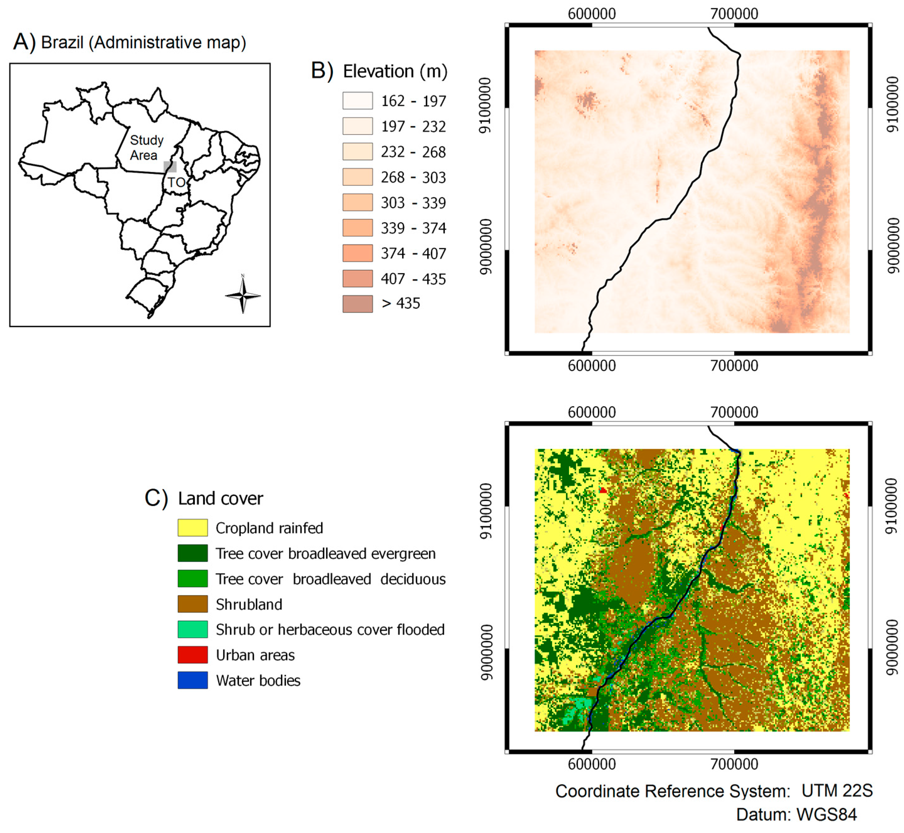
2.1. Study Area

The study area (250,000 km2) is located in the northwestern part of the Tocantins state (TO) in central Brazil extending from 7°47’–9°33′S to 48°55’–50°26′W (Figure 1) at the boundary between the savanna biome (Cerrado) and the Amazonian forest, a fire-prone region as a consequence of a flammable and dry vegetation type, and with high likelihood of human ignitions [23].
The climate is predominantly dry tropical, and characterized by a dry season from May to September [26,27]. The maximum annual temperatures vary from 22 °C in the north to 27 °C in the center-south, with precipitations varying between 1300 and 2100 mm/year [27]. The region is highly susceptible to fire risk, with the highest incidence records for the years 2005 and 2008 [28]. This site was selected as a validation study site for the ESA FIRE_CCI global burned area product [6,20,29].

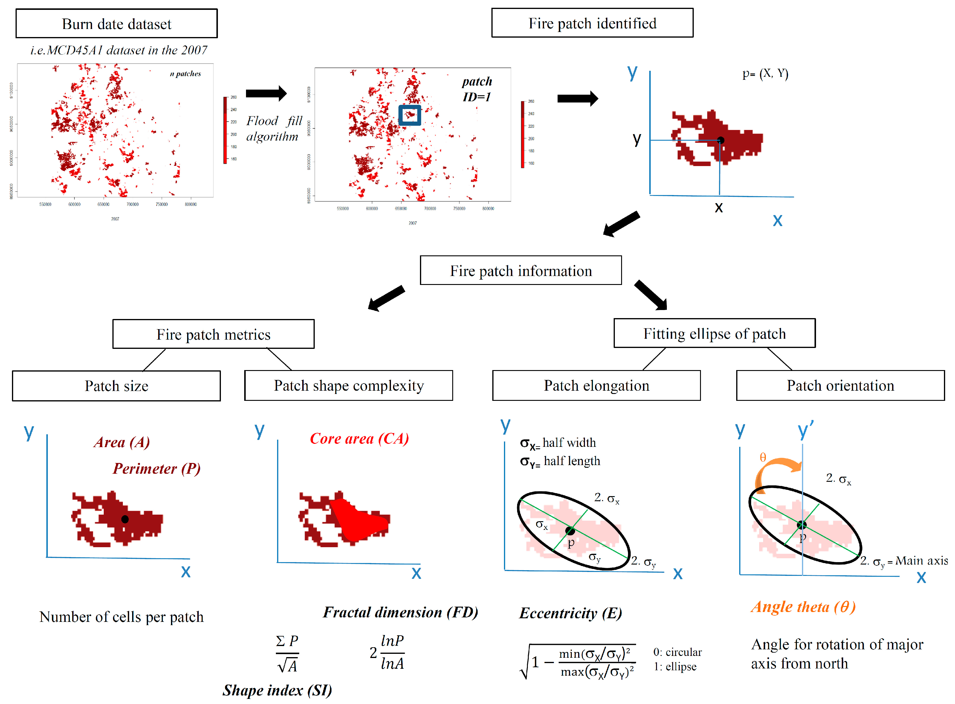
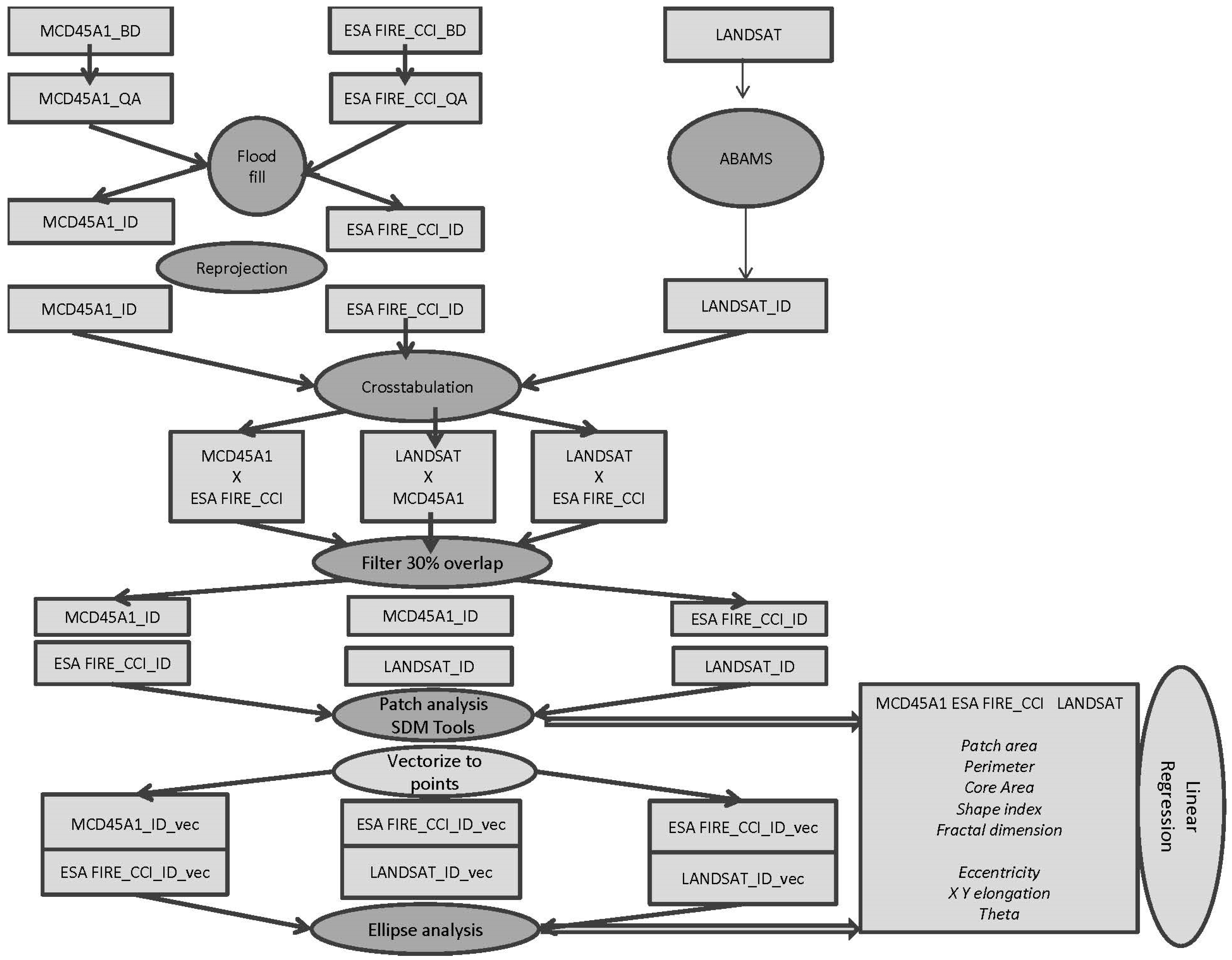
2.2. Burned Area Dataset

Among available global burned area datasets (see [3] for review), we selected MCD45A1 [21] from the MODIS sensor, and ESA FIRE_CCI [22] from the MERIS ENVISAT sensor at 500 m and 300 m resolution, respectively, in addition to the LANDSAT-derived burned patches at 30 m resolution (Table 1). The fire perimeters from LANDSAT were derived from a semi-automatic algorithm (ABAMS) [30], following a standard protocol defined for the ESA FIRE_CCI project [31], based on the CEOS-Land Product Validation guidelines [32] and used for previous global burned area products’ validation [33]. Burned area perimeters were verified by a systematic quality control through visual inspection, where all perimeters were revised visually by an external expert. Polygons where the interpretation was uncertain were labelled and the original interpreter was assisted to solve those uncertainties. For a sample of scenes and dates, a completely new interpretation was done and revised by another interpreter. Cross-tabulations between the original and the new polygons were carried out [20]. Additionally, GOFC-GOLD regional experts were contacted to provide additional information about regional problems through dedicated workshops. The LANDSAT-derived burned area perimeters should be considered a reliable source of reference information.
MCD45A1 and ESA FIRE_CCI were characterized by a burned date layer indicating the day of the year when a fire occurred, and the corresponding quality flag indicating the level of confidence in the fire occurrence varying between 0 (low confidence) to 100 (high confidence). Only the burned dates with confidence level higher than 50% were selected for MCD45A1 and ESA FIRE_CCI. All the datasets were re-projected at 30 m resolution in the UTM 22S datum WGS84 projection over the LANDSAT scene 223/066 of the Worldwide Referencing System 2 (WRS2) Path/Row. The description of the burned area time series, their spatial and temporal resolutions and their references are summarized in Table 1.
All the data statistical analysis, and the raster maps processing for the “flood-fill” algorithm, were developed and performed with R CRAN (Comprehensive R Archive Network) with the ”raster” (Geographic Data Analysis and Modeling, [34]) and “sp” (Classes and Methods for Spatial Data, [35]) packages.

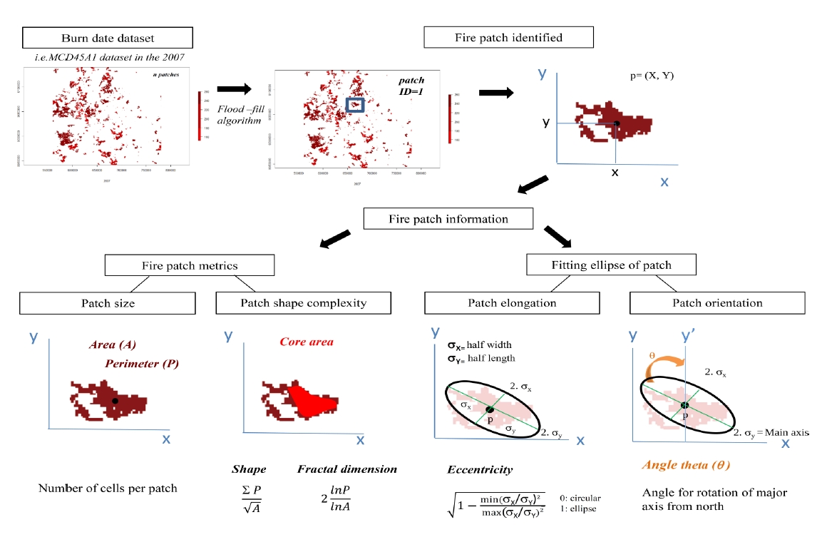
2.3. Fire Patch Identification

The burn date (BD) dataset from MCD45A1 and ESA FIRE_CCI was used to identify individual burned patches (ID), using the spatio-temporal flood fill algorithm [8]. The algorithm reads pixels BD one after the other starting from the top left corner. The first pixel with BD > 0 is assigned with ID = 1. Once a burned pixel is identified (the seed), the algorithm reads the BD values in the 8-pixel neighborhood. The neighboring pixels recorded as burned, and with a BD within a defined time interval (cut-off) with the central pixel, are classified with the same fire ID. The classification process spatially spreads out until no more neighboring burned pixel can be found within cut-off. The BD used for the patch ID classification was then removed from the BD map. The algorithm then restarts from the first pixel next to the previous seed until we reach a new burned pixel identified as ID = 2. The same flood fill process is repeated until all pixels with a BD > 0 have been assigned an individual ID code. In this work, we chose an eight day cut-off. The same algorithm was applied for ESA FIRE_CCI and MCD45A1. For LANDSAT images, ABAMS directly identified burned patches. The analysis was performed during the fire seasons for the years 2002–2009 for MCD45A1 and LANDSAT and 2006–2008 for ESA FIRE_CCI. The ID and BD maps of MCD45A1 and ESA FIRE_CCI were disaggregated to the spatial resolution of 30 m and re-projected to WGS 84 UTM 22S with the nearest neighborhood method for comparison with the LANDSAT dataset.

2.4. Fire Patch Indices and Spatial Features

From the yearly patch ID maps, where each burned pixel is referenced by its patch ID, we calculated individual patch description metrics. For each patch, we calculated its surface area (A, in m2), the length of its perimeter (P, in m) and its core area (CA in m2) corresponding to the surface area of pixels located at a given distance (we chose 500 m corresponding to the coarser pixel resolution of the BA products) inside the external boundary of a patch (buffer zone). Patch shape complexity was evaluated from its fractal dimension (FD) calculated as 2 × ln(P)/ln(A) and its shape index (SI) calculated as P/A0.5 (Table 2, Figure 2). These commonly used patch metrics in landscape ecology were first developed in the Fragstats software [36] and we used the corresponding R cran package “SDMtools” (Species Distribution Modelling Tools, [37]).
We also computed the ellipse fitting the spatial distribution of burned pixels within a patch to capture the directional azimuthal angle and the elongation of the patch, two key variables describing fire spread processes. In addition, ellipses are the theoretical shapes simulated in DGVMs, and with which they can be benchmarked. Pixels belonging to the same patch ID were converted into points with geographic coordinates corresponding to the center of the pixels. We then used the “aspace” R cran package [38] to fit the ellipse. From this ellipse, we extracted its main features including: i) the projection of the longest axis along X and Y coordinates respectively named σx and σy, ii) the eccentricity (E) as an index of patch elongation calculated as the square root of 1 minus the ratio of the squared lengths of the shortest and longest axis of the ellipse so that E = 0 corresponds to the most elongated shape, and E = 1 corresponds to a perfect circle, and iii) the theta (θ) azimuthal angle corresponding to the clockwise deviation of the longest axis of the ellipse from the northern direction (Table 2, Figure 2). These selected indices give information on the size and complexity of the fire patch, and the features of the fitted ellipse as a proxy of the theoretical fire spread simulated in DGVMs.

2.5. Data Analysis

We compared the MCD45A1, LANDSAT, and ESA FIRE_CCI BA products to each other using accuracy indices based on their patch feature relationships. Our goal here was to compare how patch morphological features are conserved between different burned area products of different spatial resolutions. However, we considered that LANDSAT burned polygons were the most accurate as they are derived from the fine tuning of a semi-automated algorithm ABAMs with much better spatial resolution than the global products (30 m versus 300–500 m) and which were thoroughly visually validated following the standards to generate a correct reference dataset [32]. We first cross tabulated yearly patch ID maps to identify overlapping patches between two sensors. For each patch ID and a given sensor, we obtained the list of the overlapping patch IDs in each of the other sensors, and the percentage of overlapping surface. When a patch in a given sensor overlapped more than one patch in the other sensor, we selected the largest patch. To test for any potential biased comparisons between patches overlapping only a few pixels, we computed the coefficient of determination R2 using a general linear model (”glm” package R cran) between overlapping patch surfaces with thresholds of overlap rates (OR%) varying from 10 to 100%. Increasing the OR threshold led to an increasing R2 of the patch size correlation for all sensor comparisons, from R2 = 0.5 for OR = 10% to R2 = 0.95 for OR = 60% and higher. We selected an OR threshold of 30% leading to patch size correlations >0.70 for further analysis (Figure 3).
We then computed linear regressions between overlapping patches with OR > 30% for each patch metric and extracted their coefficients of determination R2, p-values and slopes. The normality of the regression residuals was tested with a Shapiro-Wilk test of normality using the ”shapiro.test” from the “Stats” R cran package). When p-values of the Shapiro-Wilk test were below 0.01 indicating a significant non-normality, we log-transformed the variables and retested for the normality of the regression residuals. We log-transformed data only for the metrics of Area (A), Core Area (CA), Perimeter (P) and σx, σy in the analysis. We hypothesized that correlations might be dependent on patch size, with boundary uncertainties in global BA products affecting more importantly shape indices of small patches. We then performed regressions with the patch size thresholds >90 ha, >270 ha, >450 ha, >630 ha and >900 ha. All analyses were performed with the general linear model function “glm” in Rcran. All methodological steps are summarized in Figure 4.

3. Results

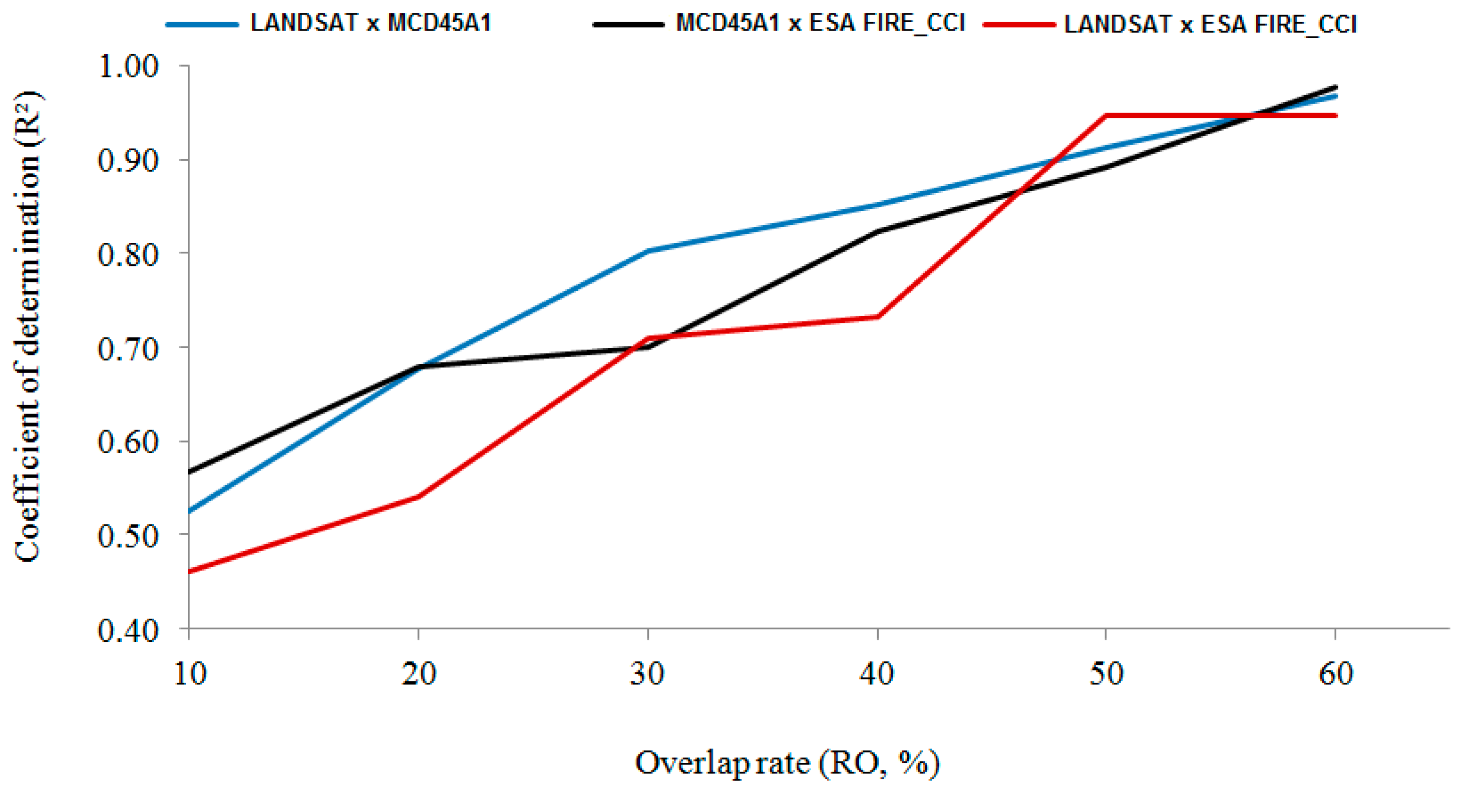
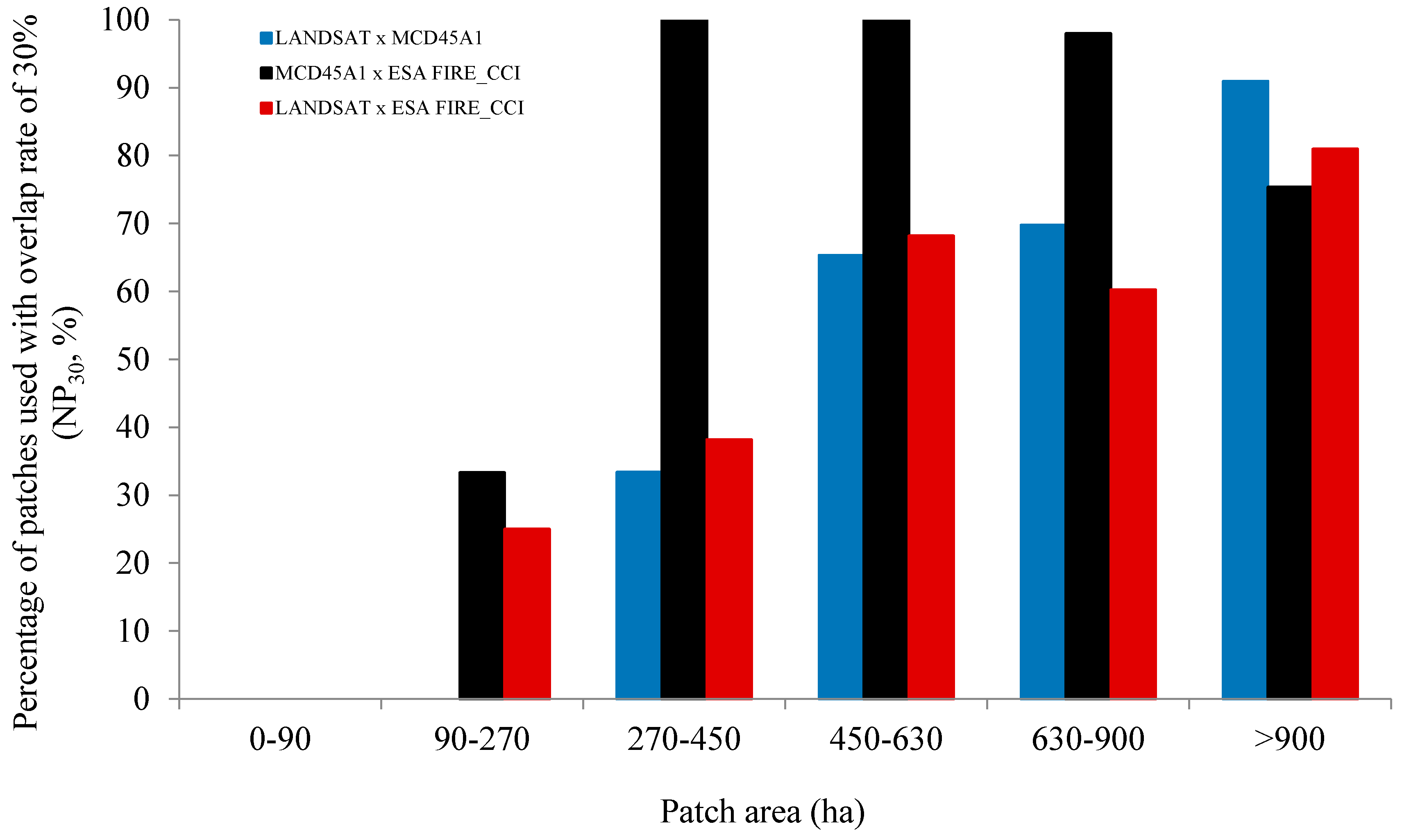
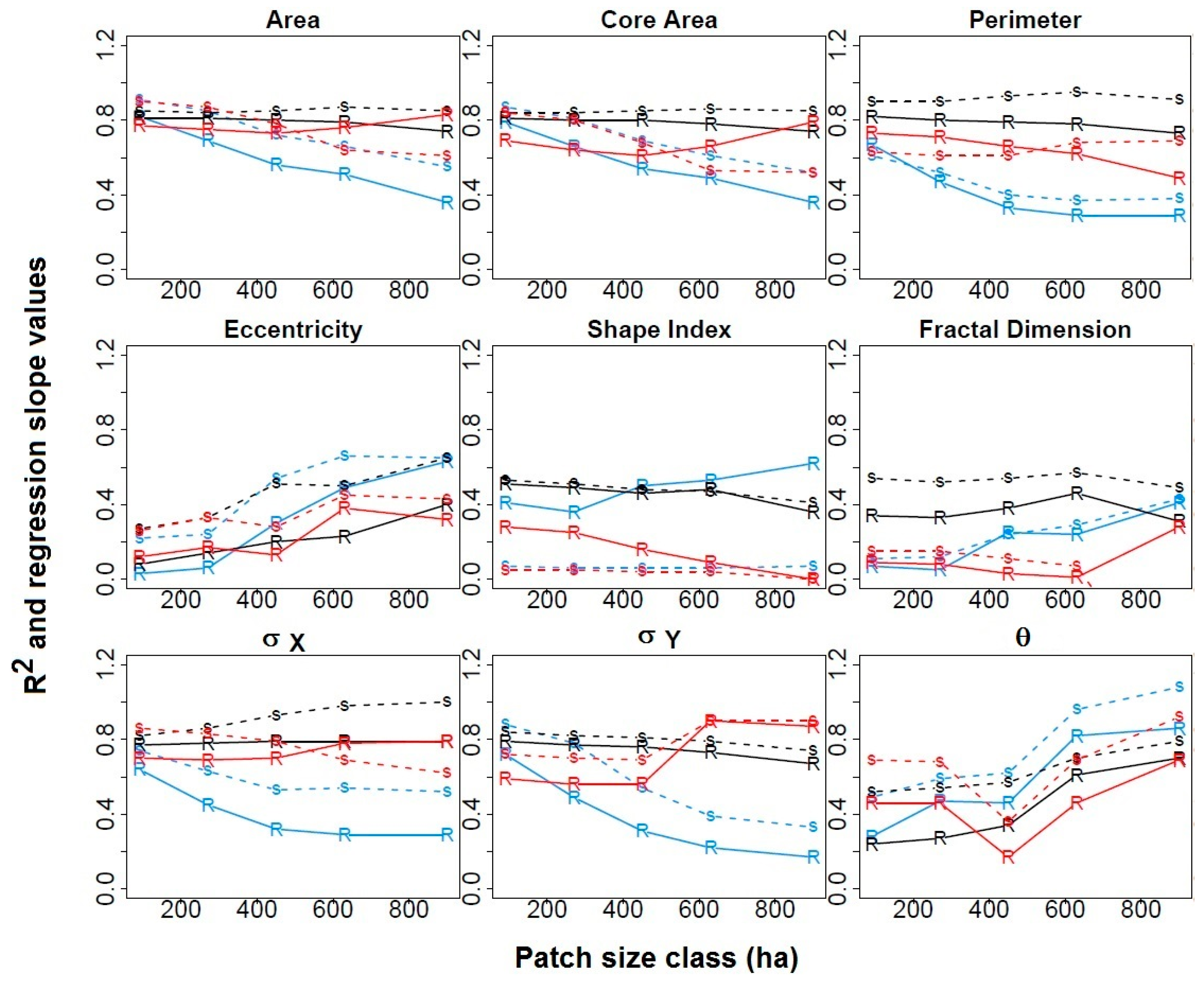
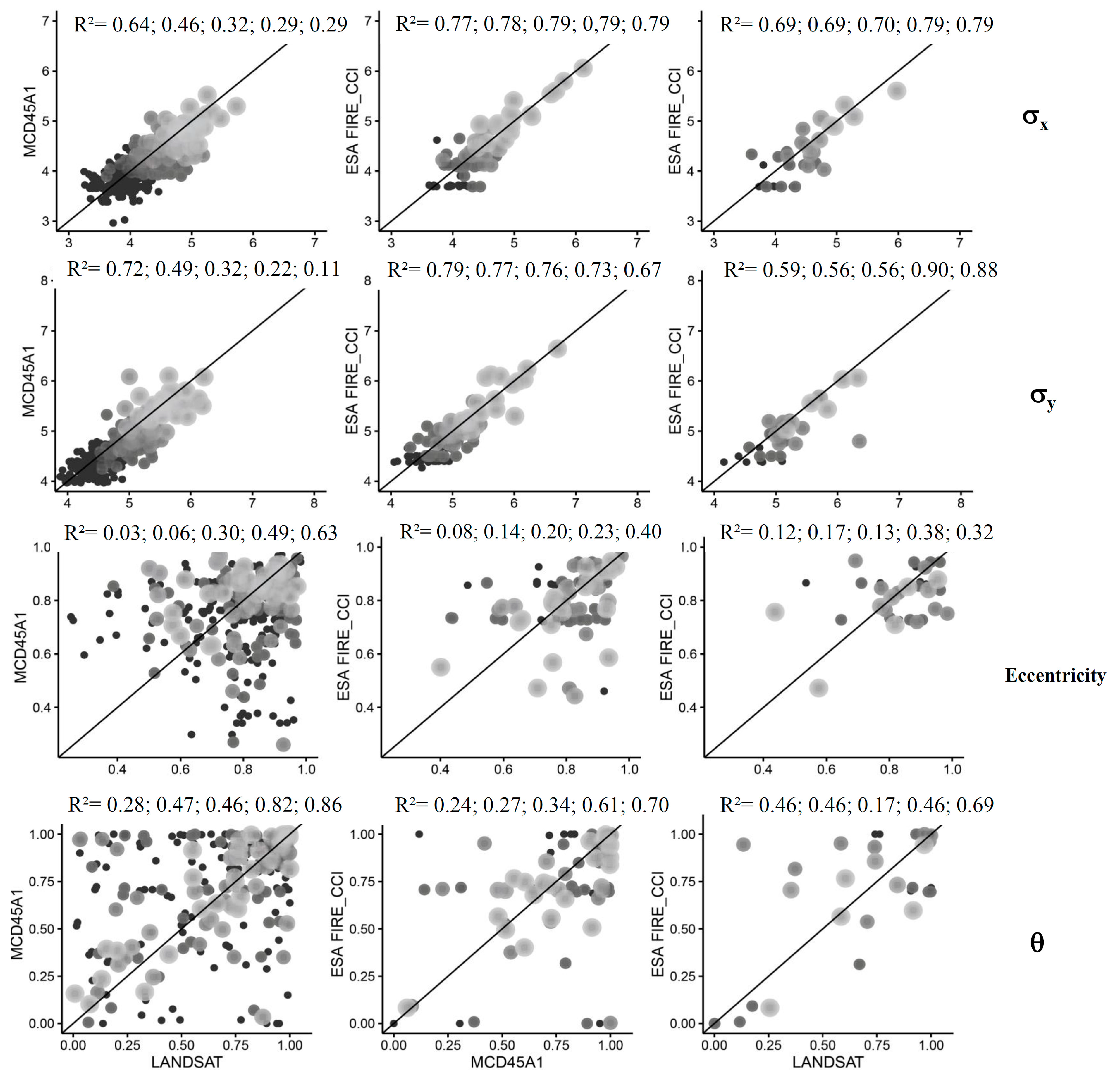
3.1. Patch Overlap between BA Products

The overall accuracy (OA) between the three BA products inter-comparisons was 0.97 (Table 3), with an omission error varying between 0.49 for the comparison between the two global products MCD45A1 and ESA FIRE_CCI, to 0.81 for the ESA FIRE_CCI × LANDSAT comparison. The commission error varied between 0.64 for the MCD45A1 × LANDSAT comparison to 0.74 for ESA FIRE_CCI × LANDSAT.
When examining the omission and commission errors for each fire size class (Table 4), we obtained higher errors (>0.9) for the smallest fire size class (<90 ha). For fire patches larger than 450 ha, OE and CE were lower than 0.6 for all comparisons. For fire patch size classes varying between 90 ha and 450 ha, OE and CE varied between 0.7 and 0.9 for the global BA products comparisons with LANDSAT. OE and CE varying between 0.4 and 0.7 for the comparison between ESA FIRE_CCI and MCD45A1.
Based on these high OE and CE values obtained for small fires, we selected only burned patches overlapping more than 30% of their surfaces. Figure 5 illustrates the percentage of patches selected after the 30% patch overlap rate (OR) threshold for each cross tabulation LANDSAT × MCD45A1, MCD45A1 × ESA FIRE_CCI and LANDSAT × ESA FIRE_CCI, and for each patch size class. We observe that all patches with a surface area lower than 90 ha were removed. We reached the threshold of 50% of patches actually analyzed in the patch size category, for all comparisons, when patches were larger than 450 ha. Above that threshold, all comparisons covered more than 60% of patches. The highest percentage of overlapping patches was obtained for the MCD45A1 × ESA FIRE_CCI comparison with more than 90% of patches actually analyzed for that 450 ha threshold. ESA FIRE_CCI and MCD45A1 comparisons with LANDSAT performed significantly worse with a percentage of analyzed patches of about 65% for patches smaller than 900 ha, but reaching 80% and 90%, respectively, for patches larger than 900 ha (Figure 5). Therefore, we can conclude that ESA FIRE_CCI and MCD45A1 BA products highly overlap for patches larger than 270 ha, but that small fires (fire patches with a surface area below 270 ha) in one product do not overlap much with the others. When comparing these global BA products with the reference LANDSAT dataset, the patch size threshold is 450 ha.

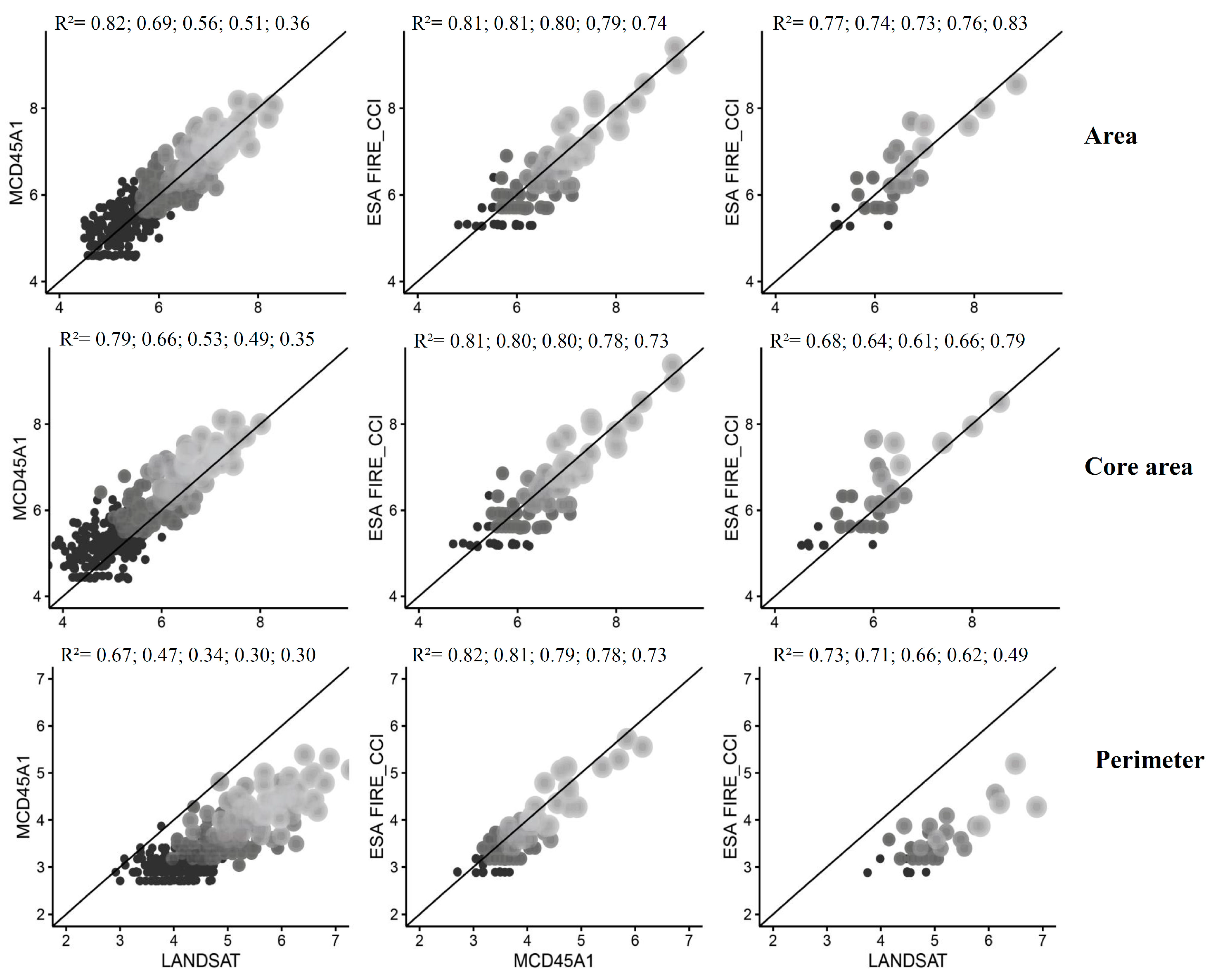
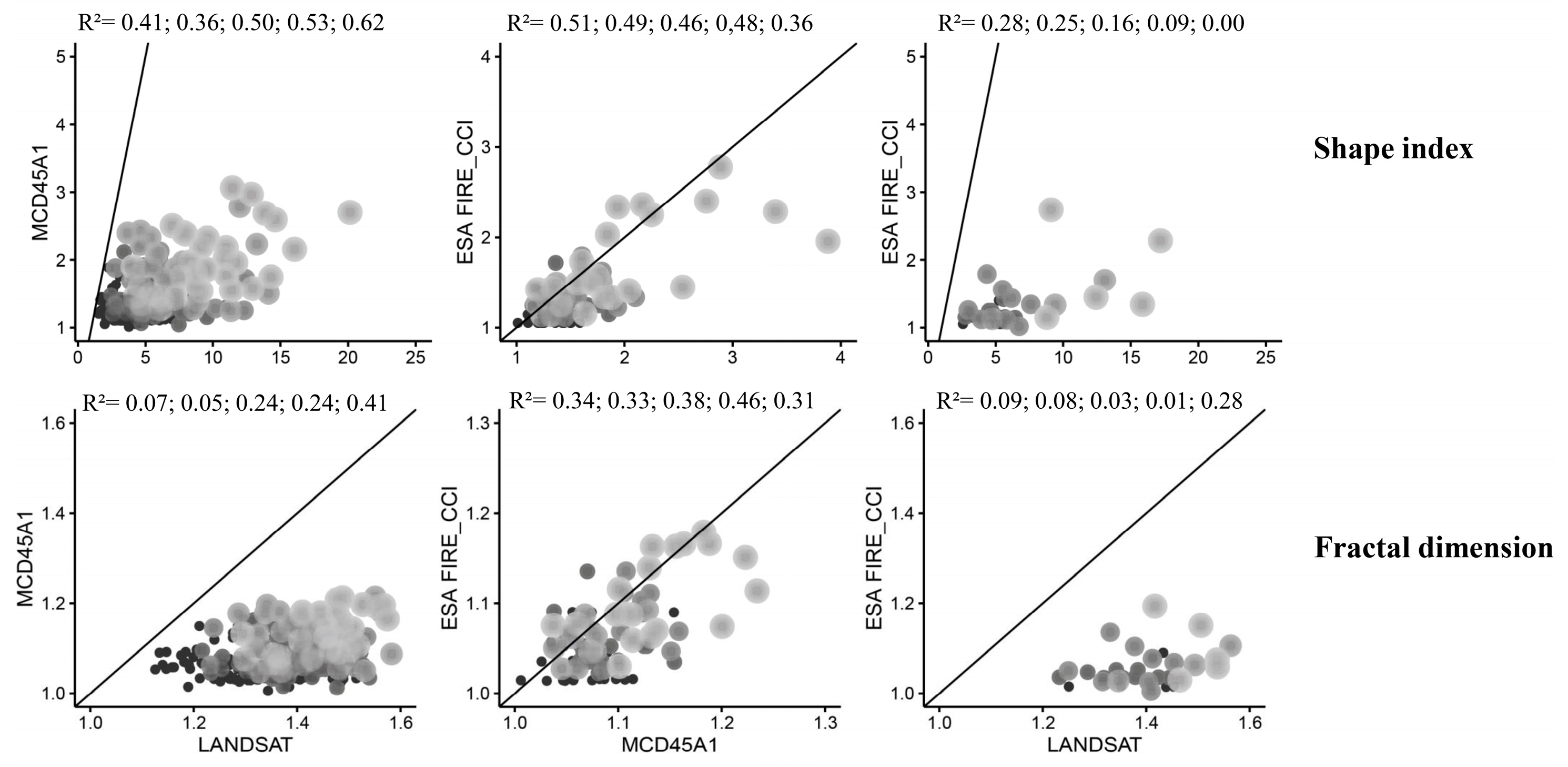
3.2. Patch Metrics Correlations

We investigated patch to patch correlations for each patch metric (Figure A1, Figure A2 and Figure A3) and Figure 6 illustrates, for each cross tabulation and patch size thresholds (Table A1), the coefficients of determination R2 indicating the fraction of the variance explained by the best-fitted linear regression, and the slopes indicating the potential bias to the 1:1 line expected if the sensors are fully conservative of the patch metrics. For the patch area, the highest R2 were obtained for the ESA FIRE_CCI × MCD45A1 (R2 > 0.8 for all patch sizes) and slopes close to 1, indicating very similar patch sizes between the two global BA products. When comparing global BA products to LANDSAT, R2 were also high for ESA FIRE_CCI (R2 > 0.8) and lower for the MCD45A1 product (R2 varies between 0.4 and 0.8). Slopes of the regression for both global BA products ESA FIRE_CCI and MCD45A1 cross-tabulated with LANDSAT varied between 0.8 for all fire size classes and 0.6 for larger fire sizes, indicating an underestimation of patch areas of similar magnitude for both global BA products. The correlation coefficients for the core area were similar to the total patch area, but with regression slopes reaching (0.6–0.9), indicating a slightly lower error in patch areas when removing the patch boundary buffer zone (500 m), where uncertainty seems to be the highest. Patch perimeters were also well correlated (R2 varying between 0.4 and 0.85) but with much higher perimeter values for LANDSAT patches performed at 30 m resolution compared to MCD45A1 and ESA FIRE_CCI performed at 500 m and 300 m, so that regression slopes vary between 0.3 and 0.65. Shape index and Fractal dimensions were correlated with R2 around 0.5 between the two global products ESA FIRE_CCI and MCD45A1 but poorly correlated when compared to LANDSAT with R2 < 0.3. The largest patches (>900 ha), however, experience better correlations for the fractal dimension (R2 > 0.4).
When analyzing the comparison of the fitted ellipse features (eccentricity and θ azimuthal direction of the longest axis), R2 were low for all comparisons, but reached values R2 > 0.3 for patches larger than 630 ha for eccentricity and R2 > 0.4 for patches larger than 630 ha for θ. Below this patch size threshold, R2 was below 0.5. Slopes of the regressions between eccentricities vary between 0.3 and 0.7 for patches larger than 450 ha, lower than the expected 1:1 line, indicating an underestimation of patch elongation and missing pixels at the extremes of patches. Slopes of the regressions for θ varied between 0.7 and 1.1 for all product comparisons, close to the expected unbiased 1:1 line.

4. Discussion

4.1. The Small Fires Issue in Global BA Products

Our results suggest some discrepancies in global BA products regarding fires smaller than 450 ha when compared to the reference finer resolution LANDSAT dataset. On one hand, the mean annual burned area covered by fire patches smaller than 270 ha represents 13.5 × 10³ ha for ESA FIRE_CCI, 22.3 × 10³ ha for MCD45A1 and 26.0 × 10³ ha for LANDSAT, out of a total burned area of 83.5 × 10³ ha for LANDSAT. Therefore, it is clear that missing burned area in global remote sensing products comes from small fires (<270 ha). For the study region, it was identified that these areas account for an average 4%–15% of the total burned area, a little lower than the usually assumed 30% of missing burned area due to missing small fires in global BA [7]. Beside this missing burned surface in global remote sensing BA products, our results particularly illustrate the little overlap between small fires (<270 ha) derived from different BA products. Below 270 ha, the percentage of patches overlapping over more than 30% of their surface between both global products ESA FIRE_CCI or MCD45A1, and the reference LANDSAT dataset was less than 40%, respectively leading to commission errors of 0.72–0.97 and omissions errors of 0.77–0.96 for this fire size class. Interestingly, however, the percentage of patches with sizes varying between 270 and 450 ha and overlapping over more than 30% of their surface between ESA FIRE_CCI and MCD45A1 was high, with omission and commission of 0.40 and 0.42 for this fire size class, indicating that both global products tend to detect the same fire patches, considered as committed when compared to LANDSAT. We might warn, however, of some issues in small fire patch detection even with the LANDSAT sensor for patches lower than 10 ha [39], so it is difficult to firmly verify the overall accuracy of global BA products on the spatial location of small patches and their extent as commissions might be the result of omitted fires from the LANDSAT analysis. Fire polygons from LANDSAT still remain the most accurate source of reference data in global burned area validation protocols, after visual [20,32,33] or field assessment [40].
The small fire issue in global BA is now well recognized for most ecosystems, as in Europe where only fires above 500 ha have been shown to be accurately captured by global products [41], with a similar threshold for Mediterranean ecosystems [42], and for China [43] or American grasslands [44]. For South American savannas, we then confirm the same missing small fires as other ecosystems, as already suggested in local studies in the region [40,45,46,47] and in other tropical savannas [48]. We then warn here of both the omission of small fire patches below 450 ha in global BA products (OE varies between 0.7 and 0.95), and, when detected, a high risk of commission (CE varies between 0.68 and 0.97). The impact on the total burned area was then compensated by omissions and commissions, but high resolution datasets delivered by global products should be used with caution at the local level for these fire types.

4.2. Uncertain Boundaries and Patch Size Underestimation

Our second main result is the underestimation of patch size for large fires. Our regressions slopes (on log transformed data) between both global BA products MCD45A1 and ESA FIRE_CCI with LANDSAT vary between 0.6 and 0.8, suggesting an underestimation of 20%–40%. This value is comparative to the results obtained for South American grasslands [49]. For the Cerrado region, a 25% underestimation [50], and up 50%–60% [40], can be observed between MCD45A1 and LANDSAT. Better correlations (regression slope = 0.94) were observed for Northern latitudes in Canada, USA for the ESA FIRE_CCI product assessment [22] while the regression slope was around 0.6 for MCD45A1 for the same region [51]. Burned patches from forest services in these latter regions, however, considered the outermost fire perimeter and might overestimate the actual burned area [52].
When using high resolution remotely sensed fire patches, patch size and patch boundary complexity have been identified as the main explanatory variables for this discrepancy when scaling up from 30 m to 1 km resolution [53,54]. Unburned patches within a fire polygon are common [17,55,56] and can significantly alter the differential reflectance at 1 km resolution so that small unburned patches at 30 m resolution can be also considered as unburned at 1 km resolution. When comparing the most used global BA products, all products have been acknowledged to underestimate burned-area and that an increase in pixel size or burned patch elongation, results in larger estimation errors [48]. This result suggests that correcting the bias on patch sizes obtained from pixel-level global remote sensing according to the slope obtained on test sites across different biomes could be further used for upscaling BA at the 0.5° final products. For a given grid cell described by its patch size distribution, the corrected total burned area would result from the sum of patch sizes corrected by the transfer function obtained in biome-specific test sites with the LANDSAT comparison, and weighted by their abundance.

4.3. Accurate Ellipse Features for Large Fires Only

Fire patch features, including patch complexity but generally patch elongation and direction, have been shown to describe a step further the burning spatial pattern and its underlying processes [57], which can be locally driven by topography, orientation of watersheds or dominant winds for example [14,15]. The quality of pixel-level global BA products to be used for characterizing the shape of fire patches and their potential response to environmental variables has rarely been assessed and these analyses have been performed only locally with high resolution fire contours. We estimated the commission and omission errors usually obtained in the quality assessments of global burned area products varied between 0.49 and 0.81 and between 0.64 and 0.74 for all fires, respectively. This result is in accordance with OE and CE observed in the region [40], and is in the highest range of uncertainty when compared to other biomes [20]. These high omission and commission values are mostly related to the high proportion of fire patches below 100 ha, as it is well known that global products (commonly based on coarse resolution sensors) tend to miss those small fires [4,7]. These OE and CE respectively decrease to 0.4–0.6 and 0.45–0.68 for fires larger than 270 ha. Ensuring that pixel-level global fire products conserve patch morphological features at 500 m resolution despite these high OE and CE would allow for global scale investigations into local processes affecting fire spread. Only the few studies listed actually compared patch features between global products and local analysis: Patch area and perimeter features for the 2005–2007 period in Greece was compared to the MCD45A1 dataset and the European Forest Fire Information System (EFFIS) [58], and illustrated how patch complexity could be largely sensor-dependent. Our results also illustrate the high discrepancy between medium resolution products (LANDSAT) and coarse resolution (500 m) global products. Previous assessments of patch metrics’ sensitivity to spatial resolution could actually illustrate contrasted responses as systematic bias or unpredictable changes [59]. The shape index and fractal dimension were among these non-consistent metrics, inherent to their resolution, so that the conservation of fire patch complexity across the spatial resolution of the different sensors is not, and will never be, attained. In our results, perimeter, shape index and fractal dimension of fire patches were poorly correlated between LANDSAT and global burned area products. However, MCD45A1 and ESA FIRE_CCI with much closer spatial resolutions were highly correlated, indicating a similar pattern of translation across scales for these two sensors.
Other aspects of patch features, and particularly their fitted ellipse, were better correlated between products. Small fires below 450 ha exhibited poor correlations for all products, actually in accordance with the low correlation of their patch size discussed above. For fires larger than 450 ha, we could, however, conclude with fair agreement on patch azimuthal orientation and patch elongation, both increasingly growing with fire size, suggesting an accurate conservation of patch features in global remote sensing products to be used for model benchmarking, and confirming early results obtained from the ESA FIRE_CCI product for Northern latitudes [22].

4.4. Implications for Pyrogeography and DGVM Benchmarking

We investigated here the ability of global remote sensing products, with their pixel-level information, to provide keystone information on fire regimes, as already initiated with fire size distribution [60,10] and further used for better fire risk modelling in Amazonia [61]. Patch complexity, elongation and orientation have been chosen as keystone features related to fire spread processes leading to the final fire shape, and the inherent fire intensity. Demonstrating that global burned area products from remote sensing conserve the main features of fire shapes, at least for this study site representative of the fire prone South American savanna, should encourage the further use of the pixel level product to calculate patch shape indices. Defining a fire by its morphological or spreading traits, and a fire regime by its assemblage of fires defined by their traits could make the link with analytical tools of the emerging functional biogeography [62]. The main constraint would be the limit in considering only fires larger than 450 ha, and the sensitivity of fire patch individuation to the cut-off time span used in the flood fill algorithm [63]. Increased resolution in global fire products might, however, strengthen our results for small fires in the near future.
Understanding the spatial and temporal pattern of fire patch features from global remote sensing would finally extend the potential global DGVM benchmarking mostly performed on burned areas [6]. DGVMs were indeed more recently evaluated, also in terms of fire size distribution [11], and were increasingly oriented to fire shape metrics and fire spread processes [64]. For example, fire intensity can be related to fire patch features as the ratio between core area/area index [65] or fire patch elongation [66], when coupled with fire line intensity, as a function of fuel biomass and water status, and fire rate of spread. Recently, this fire rate of spread within fire patches has been investigated according to burn dates from pixel products of global BA or hotspots [67,68,69] and for which the accuracy in the timing of burn dates has been investigated [70], and establish here the forthcoming developments in global fire analysis and modeling.

5. Conclusions

We performed a full intercomparison of two commonly used global burned area products [3] with a local evaluation based on LANDSAT images at fine resolution. To do so, we analyzed the morphological features of fire patches derived from the pixel-level information of ‘burn date’ delivered by two global burned area products (MCD45A1 and ESA FIRE_CCI), a neglected aspect of these products’ quality assessments. Our results confirm earlier findings about the underestimation of burned areas from global remote sensing due to the omission of small fires, but also highlight the potential underestimation of burned areas at the patch level as a consequence of high uncertainty in the patch boundary. However, the patch core area derived from global remote sensing seems conservative as well as the general fire shape, a key finding for further analysis of fire regimes and intrinsic processes, and for better DGVM benchmarking. We suggest here to develop further analysis at the global scale as initiated by [22] and develop statistical frameworks for the comparison of fire patch features.

Acknowledgments

This work was developed within the Fire-CCI project, in the framework of the European Space Agency Climate Change Initiative program and the IRD/CNPq collaborative agreement program. The Coordenação de Aperfeiçoamento de Pessoal Superior (CAPES, Brazil) provided a PhD grant to Joana Nogueira (BEX-1185-13-6 process). Julien Ruffault was supported by a post-doctoral grant within the European Community’s Seventh Framework Program (CLARIS-LPB, Grant Agreement No 212492).

Author Contributions

J.M.P.N. and F.M. designed the experiment. J.M.P.N. performed the analysis and led the study. E.C. provided burned area from remote sensing. J.R. processed the burn dates into patches. J.M.P.N. and F.M. wrote the paper.

Conflicts of Interest

The authors declare no conflict of interest.

Appendix A

Figure A1. Correlations of (log transformed) patch metrics (Area in m2, Core area in m2, and Perimeter in m) for comparison: 1—LANDSAT × MCD45A1, 2—MCD45A1 × ESA FIRE_CCI and 3—LANDSAT × ESA FIRE_CCI. The grey scale color of individual points correspond to their patch size class from 90ha (black), 270ha, 450ha, 630ha, to 900 ha (light grey).The R squared values indicate the coefficient of determination ordered in according to patch size class.
Remotesensing 09 00007 g007
Figure A2. Correlations of patch metrics (Shape Index and Fractal Dimension) for comparison: 1—LANDSAT × MCD45A1, 2—MCD45A1 × ESA FIRE_CCI and 3—LANDSAT × ESA FIRE_CCI. The grey scale color of individual points correspond to their patch size class from 90 ha (black), 270 ha, 450 ha, 630 ha, to 900 ha (light grey). The R squared values indicate the coefficient of determination ordered in according to patch size class.
Remotesensing 09 00007 g008
Figure A3. Correlations of the ellipse metrics, fitted over fire patches (shortest and longest axis σx and σy (log transformed), eccentricity and azimuthal angle of the longest axis theta) for comparison: 1—LANDSAT × MCD45A1, 2—MCD45A1 × ESA FIRE_CCI and 3—LANDSAT × ESA FIRE_CCI. The grey scale color of individual points correspond to their patch size class from 90 ha (black), 270 ha, 450 ha, 630 ha, to 900 ha (light grey). R2 values indicate the coefficient of determination of the regressions, ordered according to the patch size classes.
Remotesensing 09 00007 g009
Table A1. Slope (S) and determination (R2) coefficients of linear regression for patch metrics in each comparison among fire products.
SizeShapeOrientationArea (ha)Comparison
AreaCore AreaPerimeterEccentricityShape IndexFractal DimensionX SigmaY SigmaTheta
R20.82 **0.79 ***0.67 ***0.03 *0.41 ***0.07 ***0.64 ***0.72 ***0.28 ***>90LANDSAT × MCD45A1
0.69 ***0.66 ***0.47 ***0.060.36 ***0.050.46 ***0.49 ***0.47 ***>270
0.56 ***0.53 ***0.34 ***0.30 ***0.50 ***0.24 **0.32 ***0.32 ***0.46 ***>450
0.51 ***0.49 **0.30 ***0.49 **0.53 **0.240.29 ***0.22 **0.82 ***>630
0.36 *0.350.30 **0.63 *0.62 *0.410.29 **0.110.86 ***>900
S0.91 ***0.87 ***0.61 ***0.22 *0.07 ***0.11 ***0.74 ***0.88 ***0.49 ***>90
0.85 ***0.81 ***0.52 ***0.240.06 ***0.120.63 ***0.78 ***0.59 ***>270
0.73 ***0.69 ***0.40 ***0.54 ***0.06 ***0.24 **0.53 ***0.55 ***0.62 ***>450
0.66 ***0.61 **0.38 ***0.66 **0.06 **0.290.54 ***0.39 **0.96 ***>630
0.55 *052 ***0.38 **0.65 *0.07 *0.430.52 **0.33 NS1.08 ***>900
R20.81 ***0.81 ***0.82 ***0.08 ***0.51 ***0.34 ***0.77 ***0.79 ***0.24 ***>90MCD45A1 × ESA FIRE_CCI
0.81 ***0.80 ***0.81 ***0.14 ***0.49 ***0.33 ***0.78 ***0.77 ***0.27 ***>270
0.80 ***0.80 ***0.79 ***0.201 ***0.46 ***0.38 ***0.79 ***0.76 ***0.34 ***>450
0.79 ***0.78 ***0.78 ***0.23 ***0.48 ***0.46 ***0.79 ***0.73 ***0.61 ***>630
0.74 ***0.73 ***0.73 ***0.40 ***0.36 ***0.31 **0.79 ***0.67 ***0.70 ***>900
S0.85 ***0.84 ***0.90 ***0.27 ***0.53 ***0.54 ***0.82 ***0.84 ***0.52 ***>90
0.84 ***0.84 ***0.91 ***0.33 ***0.51 ***0.52 ***0.87 ***0.82 ***0.54 ***>270
0.85 ***0.85 ***0.93 ***0.51 ***0.48 ***0.54 ***0.93 ***0.80 ***0.57 ***>450
0.87 ***0.87 ***0.95 ***0.50 ***0.47 ***0.57 ***0.98 ***0.79 ***0.70 ***>630
0.85 ***0.85 ***0.92 ***0.65 ***0.41 ***0.49 **1.03 ***0.74 ***0.79 ***>900
R20.77 ***0.68 ***0.73 ***0.12 **0.28 ***0.09 *0.69 ***0.59 ***0.46 ***>90LANDSAT × ESA FIRE_CCI
0.74 ***0.64 ***0.71 ***0.17 **0.25 ***0.080.69 ***0.56 ***0.46 ***>270
0.73 ***0.61 ***0.66 ***0.130.160.030.70 ***0.56 **0.17NS>450
0.76 ***0.66 ***0.62 **0.380.090.010.79 ***0.90 ***0.46 *>630
0.83 ***0.79 ***0.490.320.000.280.79 **0.88 **0.69 *>900
S0.90 ***0.84 ***0.62 ***0.26 **0.05 ***0.15 *0.86 ***0.72 ***0.69 ***>90
0.86 ***0.80 ***0.61 ***0.33 **0.05 ***0.150.83 ***0.70 ***0.68 ***>270
0.78 ***0.68 ***0.61 ***0.280.040.110.79 ***0.69 **0.36>450
0.64 ***0.53 ***0.68 **0.450.040.070.69 ***0.90 ***0.69 *>630
0.61 ***0.53 ***0.690.43−0.0004−0.700.62 **0.90 **0.92 *>900
The R2 and S coefficients are significant values in p < 0.01 (***), p < 0.05 (**) and p < 0.1 (*). For the comparison among LANDSAT and MCD45A1 products, the values before and after the parentheses are equivalent for 2006–2008 and for 2002–2009, respectively.

References

  1. Yue, C.; Ciais, P.; Zhu, D.; Wang, T.; Peng, S.S.; Piao, S.L. How have past fire disturbances contributed to the current carbon balance of boreal ecosystems? Biogeosciences 2016, 13, 675–690. [Google Scholar] [CrossRef] [Green Version]
  2. Hao, W.M.; Liu, M.H. Spatial and temporal distribution of tropical biomass burning. Glob. Biogeochem. Cycles 1994, 8, 495–503. [Google Scholar] [CrossRef]
  3. Mouillot, F.; Schultz, M.G.; Yue, C.; Cadule, P.; Tansey, K.; Ciais, P.; Chuvieco, C. Ten years of global burned area products from spaceborne remote sensing—A review: Analysis of user needs and recommendations for future developments. Int. J. Appl. Earth Obs. Geoinf. 2014, 26, 64–79. [Google Scholar] [CrossRef]
  4. Giglio, L.; Randerson, J.T.; Werf, G.R. Analysis of daily, monthly, and annual burned area using the fourth generation global fire emissions database (GFED4). J. Geophys. Res. Biogeosci. 2013, 118, 317–328. [Google Scholar] [CrossRef]
  5. Hantson, S.; Arneth, A.; Harrison, S.P.; Kelley, D.I.; Prentice, I.C.; Rabin, S.S.; Archibald, S.; Mouillot, F.; Arnold, S.R.; Artaxo, P.; et al. The status and challenge of global fire modelling. Biogeosciences 2016, 13, 3359–3375. [Google Scholar] [CrossRef]
  6. Padilla, M.; Stehman, S.V.; Ramo, R.; Corti, D.; Hantson, S.; Oliva, P.; Alonso, I.C.; Bradlev, A.V.; Tansey, K.; Mota, B.; et al. Comparing the accuracies of remote sensing global burned area products using stratified random sampling and estimation. Remote Sens. Environ. 2015, 160, 114–121. [Google Scholar] [CrossRef]
  7. Randerson, J.T.; Chen, Y.; van der Werf, G.R.; Rogers, B.M.; Morton, D.C. Global burned area and biomass burning emissions from small fires. J. Geophys. Res. Biogeosci. 2012, 117, 21456–22202. [Google Scholar] [CrossRef]
  8. Loepfe, L.; Rodrigo, A.; Lloret, F. Two thresholds determine climatic control of forest fire size in Europe and North Africa. Reg. Environ. Change 2014, 14, 1395–1404. [Google Scholar] [CrossRef]
  9. Archibald, S.; Roy, D.P. Identifying individual fires from satellite-derived burned area data. In Proceedings of the IEEE International Geoscience and Remote Sensing Symposium, Cape Town, South Africa, 12–17 July 2009. [CrossRef]
  10. Hantson, S.; Pueyo, S.; Chuvieco, E. Global fire size distribution is driven by human impact and climate. Glob. Ecol. Biogeogr. 2015, 24, 77–86. [Google Scholar] [CrossRef]
  11. Yue, C.; Ciais, P.; Cadule, P.; Thonicke, K.; Archibald, S.; Poulter, B.; Hao, W.M.; Hantson, S.; Mouillot, F.; Friedlingstein, P.; et al. Modelling the role of fires in the terrestrial carbon balance by incorporating SPITFIRE into the global vegetation model ORCHIDEE–Part 1: Simulating historical global burned area and fire regime. Geosci. Model Dev. 2014, 7, 2747–2767. [Google Scholar] [CrossRef] [Green Version]
  12. Rothermel, R.C. A Mathematical Model for Predicting Fire Spread in Wildland Fuels; US Department of Agriculture, Forest Service, Intermountain Forest and Range Experiment Station: Ogden, UT, USA, 1972.
  13. Cary, G.J.; Keane, R.E.; Gardner, R.H.; Lavorel, S.; Flannigan, M.D.; Davies, I.D.; Li, C.; Lenihan, J.M.; Rupp, T.S.; Mouillot, F. Comparison of the sensitivity of landscape-fire-succession models to variation in terrain, fuel pattern, climate and weather. Landsc. Ecol. 2006, 21, 121–137. [Google Scholar] [CrossRef]
  14. Barros, A.M.G.; Pereira, J.M.C.; Lund, U.J. Identifying geographical patterns of wildfire orientation: A watershed based analysis. For. Ecol. Manage. 2012, 264, 98–107. [Google Scholar] [CrossRef]
  15. Barros, A.M.G.; Pereira, J.M.C.; Moritz, M.A.; Stephens, S.L. Spatial characterization of wildfire orientation patterns in California. Forests 2013, 4, 197–217. [Google Scholar] [CrossRef]
  16. Oliveira, S.L.J.; Campagnolo, M.L.; Price, O.F.; Edwards, A.C.; Smith, J.R.; Pereira, J.M.C. Ecological implications of fine scale fire patchiness and severity in tropical savannas of northern Australia. Fire Ecol. 2015, 11, 10–31. [Google Scholar] [CrossRef]
  17. Roman-Cuesta, R.M.; Gracia, M.; Retana, J. Factors influencing the formation of unburned forest islands within the perimeter of a large forest fire. For. Ecol. Manage. 2009, 258, 71–80. [Google Scholar] [CrossRef]
  18. O’Neill, R.V.; Krummel, J.R.; Gardner, R.H.; Sugihara, G.; Jackson, B.; Angelis, D.L.; Milne, B.T.; Turner, M.G.; Zygmut, B.; Chistensen, S.W.; et al. Indices of landscape pattern. Landsc. Ecol. 1988, 1, 153–162. [Google Scholar]
  19. Takaoka, S.; Sasa, K. Landform effects on fire behavior and post fire regeneration in the mixed forests of northern Japan. Ecol. Res. 1996, 11, 339–349. [Google Scholar] [CrossRef]
  20. Padilla, M.; Stehman, S.V.; Litago, J.; Chuvieco, E. Assessing the temporal stability of the accuracy of a time series of burned area products. Remote Sens. 2014, 6, 2050–2068. [Google Scholar] [CrossRef]
  21. Roy, D.P.; Boschetti, L.; Justice, C.O.; Ju, J. The collection 5 MODIS burned area product—Global evaluation by comparison with the MODIS active fire product. Remote Sens. Environ. 2008, 112, 3690–3707. [Google Scholar] [CrossRef]
  22. Chuvieco, E.; Yue, C.; Heil, A.; Mouillot, F.; Alonso-Canas, I.; Padilla, M.; Pereira, J.M.; Oom, D.; Tansey, K. A new global burned area product for climate assessment of fire impacts. Glob. Ecol. Biogeogr. 2016, 25, 619–629. [Google Scholar] [CrossRef]
  23. Viergever, M. Plano Estadual de Controle de Queimadas e Combate a Incêndios Florestais. Governo do Estado do Tocantins: Brasilia, Brazil, 2009. Available online: http://www.fundoamazonia.gov.br/ FundoAmazonia/export/sites/default/site_pt/Galerias/Arquivos/Publicacoes/Plano_Estadual_do_Tocantins.pdf (accessed on 5 June 2016). [Google Scholar]
  24. Jarvis, A.; Reuter, H.I.; Nelson, A.; Guevara, E. Hole-Filled Seamless SRTM Data V4; International Centre for Tropical Agriculture (CIAT): Palmira, Colombia, 2008. [Google Scholar]
  25. ESA—European Space Agency. CCI Land Cover Product User Guide Version 2.4; ESA: Paris, France, 2014. [Google Scholar]
  26. Instituto Brasileiro de Geografia e Estatística. Available online: http://www.ibge.gov.br/ (accessed on 5 June 2016).
  27. Instituto Nacional de Pesquisas Espaciais. Available online: http://www.inpe.br/ (accessed on 5 June 2016).
  28. Ministério do Meio Ambiente. Available online: http://www.mma.gov.br/ (accessed on 5 June 2016).
  29. Hantson, S.; Padilla, M.; Corti, D.; Chuvieco, E. Strengths and weaknesses of MODIS hotspots to characterize global fire occurrence. Remote Sens. Environ. 2013, 131, 152–159. [Google Scholar] [CrossRef]
  30. Bastarrika, A.; Alvarado, M.; Artano, K.; Martinez, M.; Mesanza, A.; Torre, L.; Ramo, R.; Chuvieco, E. BAMS: A tool for supervised burned area mapping using Landsat data. Remote Sens. 2014, 6, 12360–12380. [Google Scholar] [CrossRef]
  31. Padilla, M.; Chuvieco, E.; Hantson, S.; Theis, R.; Sandow, C. ESA FIRE CCI Product Validation Plan. 2011. Available online: http://www.esa-fire-cci.org/webfm_send/241 (accessed on 23 December 2016).
  32. Boschetti, L.; Roy, D.; Justice, C. International Global Burned Area Satellite Product Validation Protocol Part I—Production and Standardization of Validation Reference Data; Committee on Earth Observation Satellites: Maryland, MD, USA, 2009. [Google Scholar]
  33. Roy, D.P.; Boschetti, L. Southern Africa validation of the MODIS, L3JRC and GlobCarbon burned-area products. IEEE Trans. Geosci. Remote Sens. 2009, 47, 1032–1044. [Google Scholar] [CrossRef]
  34. Hijmans, R.J. Raster: Geographic Data Analysis and Modeling. R Package Version 2.2-31. Available online: http://CRAN.R-project.org/package=raster/ (accessed on 3 March 2016).
  35. Pebesma, E.J.; Bivand, R.S. Classes and Methods for Spatial Data in R. R News 5 (2). Available online: http://cran.r-project.org/doc/Rnews/ (accessed on 3 March 2016).
  36. McGarigal, K.; Marks, B.J. FRAGSTATS: Spatial Pattern Analysis Program for Quantifying Landscape Structure V.2; USDA Forest Service: Portland, OR, USA, 1995.
  37. Vanderwal, J.; Falconi, L.; Januchowski, S.; Shoo, L.; Storlie, C. Species Distribution Modelling Tools (SDMTools): Tools for Processing daTa Associated with Species Distribution Modelling Exercises. R Package Version 1.1-20. Available online: http://CRAN.R-project.org/package=SDMTools/ (accessed on 3 March 2016).
  38. Bui, R.; Buliung, R.N.; Remmel, T.K. Aspace: A Collection of Functions for Estimating Centrographic Statistics and Computational Geometries for Spatial Point Patterns. R Package Version 3.2. Available online: http://CRAN.R-project.org/package=aspace (accessed on 3 March 2016).
  39. Boschetti, L.; Roy, D.P.; Justice, C.O.; Humber, M.L. MODIS Landsat fusion for large area 30m burned area mapping. Remote Sens. Environ. 2015, 161, 27–42. [Google Scholar] [CrossRef]
  40. Libonati, R.; DaCamara, C.C.; Setzer, A.W.; Morelli, F.; Melchiori, A.E. An algorithm for burned area detection in the Brazilian Cerrado using 4 µm MODIS imagery. Remote Sens. 2015, 7, 15782–15803. [Google Scholar] [CrossRef]
  41. Vilar, L.; Camia, A.; San-Miguel-Ayanz, J. A comparison of remote sensing products and forest fire statistics for improving fire information in Mediterranean Europe. Eur. J. Remote Sens. 2015, 48, 345–364. [Google Scholar] [CrossRef]
  42. Levin, N.; Heimowitz, A. Mapping spatial and temporal patterns of Mediterranean wildfires from MODIS. Remote Sens. Environ. 2012, 126, 12–26. [Google Scholar] [CrossRef]
  43. Li, J.; Song, Y.; Huang, X.; Mengmeng, L. Comparison of burned areas in mainland China derived from MCD45A1 and data recorded in yearbooks from 2001 to 2011. Int. J. Wildland Fire 2014, 24, 103–113. [Google Scholar] [CrossRef]
  44. Sunderman, S.O.; Weiberg, P.J. Remote sensing approaches for reconstructing fire perimeters and burn severity mosaics in desert spring ecosystems. Remote Sens. Environ. 2011, 115, 2384–2389. [Google Scholar] [CrossRef]
  45. Oliveras, I.; Anderson, L.O.; Malhi, Y. Application of remote sensing to understanding fire regimes and biomass burning emissions of the tropical Andes. Glob. Biogeochem. Cycles. 2014, 28, 480–496. [Google Scholar] [CrossRef]
  46. Cardozo, F.S.; Pereira, G.; Shimabukuro, Y.E.; Moraes, E.C. Analysis and assessment of the spatial and temporal distribution of burned areas in the Amazon forest. Remote Sens. 2014, 6, 8002–8025. [Google Scholar] [CrossRef]
  47. Bradley, A.V.; Millington, A.C. Spatial and temporal scale issues in determining biomass burning regimes in Bolivia and Peru. Int. J. Remote Sens. 2006, 27, 2221–2253. [Google Scholar] [CrossRef]
  48. Anaya, J.A.; Chuvieco, E. Accuracy assessment of burned area products in the Orinoco basin. Photogramm. Eng. Remote Sens. 2012, 78, 53–60. [Google Scholar] [CrossRef]
  49. Hardtke, L.A.; Blanco, P.D.; del Valle, H.F.; Metternicht, G.I.; Sione, W.F. Semi automated mapping of burned areas in semiarid ecosystems using MODIS time series imagery. Int. J. Appl. Earth Obs. Geoinf. 2015, 38, 25–35. [Google Scholar] [CrossRef]
  50. Araujo, F.M.; Ferreira, L.G. Satellite base automated burned area detection: A performance assessment of the MODIS MCD45A1 in the Brazilian savanna. Int. J. Appl. Earth Obs. Geoinf. 2015, 36, 94–102. [Google Scholar] [CrossRef]
  51. Chang, D.; Song, Y. Comparison of L3JRC and MODIS global burned area products 2000 to 2007. J. Geophys. Res. Atmos. 2009, 114, 2156–2202. [Google Scholar] [CrossRef]
  52. Giglio, L.; van der Werf, G.R.; Randerson, J.T.; Collatz, G.J.; Kasibhatla, P. Global estimation of burned area using MODIS active fire observations. Atmos. Chem. Phys. 2006, 6, 957–974. [Google Scholar] [CrossRef] [Green Version]
  53. Silva, J.M.N.; Sa, A.C.L.; Pereira, J.M.C. Comparison of burned area estimates derived from SPOT VEGETATION and Landsat ETM+ data in Africa: Influence of spatial pattern and vegetation type. Remote Sens. Environ. 2005, 96, 188–201. [Google Scholar] [CrossRef]
  54. Sa, A.C.L.; Pereira, J.M.C.; Gardner, R.H. Analysis of the relationship between spatial pattern and spectral detectability of areas burned in southern Africa using satellite data. Int. J. Remote Sens. 2007, 28, 3583–3601. [Google Scholar] [CrossRef]
  55. Andison, D.W. The influence of wildfire boundary delineation on our understanding of burning patterns in the Alberta foothills. Can. J. For. Res. 2012, 42, 1253–1263. [Google Scholar] [CrossRef]
  56. Kolden, C.A.; Lutz, J.A.; Key, C.H.; Kane, J.T.; van Wagtendonk, J.W. Mapped versus actual burned area within wildfire perimeters: Characterizing the unburned. For. Ecol. Manage. 2012, 286, 38–47. [Google Scholar] [CrossRef]
  57. Baker, W.L. The landscape ecology of large disturbances in the design and management of nature reserves. Landsc. Ecol. 1992, 7, 181–194. [Google Scholar] [CrossRef]
  58. Kalivas, D.P.; Petropoulos, G.P.; Athanasiou, I.M.; Kollias, V.J. An intercomparison of burnt area estimates derived from key operational products: The Greek wildland fires of 2005–2007. Nonlinear Proc. Geophys. 2013, 20, 397–409. [Google Scholar] [CrossRef]
  59. Wu, J.G. Effects of changing scale on landscape pattern analysis: Scaling relations. Landsc. Ecol. 2004, 19, 125–138. [Google Scholar] [CrossRef]
  60. Archibald, S.; Scholes, R.J.; Roy, D.P.; Roberts, G.; Boschetti, L. Southern African fire regimes as revealed by remote sensing. Int. J. Wildland Fire 2010, 19, 861–878. [Google Scholar] [CrossRef]
  61. Fletcher, I.N.; Aragao, L.E.O.C.; Lima, A.; Shimabukuro, Y.; Friedlingstein, P. Fractal properties of forest fires in Amazonia as a basis for modelling pan tropical burnt area. Biogeosciences 2014, 11, 1449–1459. [Google Scholar] [CrossRef] [Green Version]
  62. Violle, C.; Reich, P.B.; Pacala, S.W.; Enquist, B.J.; Kattge, J. The emergence and promise of functional biogeography. Proc. Natl. Acad. Sci. USA 2014, 111, 13690–13696. [Google Scholar] [CrossRef] [PubMed]
  63. Oom, D.; Silva, P.C.; Bistinas, I.; Pereira, J.M.C. Highlighting biome specific sensitivity of fire size distributions to time-gap parameters using a new algorithm for fire event individuation. Remote Sens. 2016, 8. [Google Scholar] [CrossRef]
  64. Duff, T.J.; Chong, D.M.; Tolhurst, K.G. Quantifying spatio temporal differences between fire shapes: Estimating fire travel paths for the improvement of dynamic spread models. Environ. Model. Softw. 2013, 46, 33–43. [Google Scholar] [CrossRef]
  65. Cansler, C.A.; McKenzie, D. Climate, fire size and biophysical setting control fire severity and spatial pattern in the northern Cascade Range, USA. Ecol. Appl. 2014, 24, 1037–1056. [Google Scholar] [CrossRef] [PubMed]
  66. Catchpole, E.A.; Alexander, M.E.; Gill, A.M. Elliptical-fire perimeter and area-intensity distributions. Can. J. For. Res. 1992, 22, 968–972. [Google Scholar] [CrossRef]
  67. Collins, B.M.; Kelly, M.; van Wagtendonk, J.W.; Stephens, S.L. Spatial patterns of large natural fires in Sierra Nevada wilderness areas. Landsc. Ecol. 2007, 22, 545–557. [Google Scholar] [CrossRef]
  68. Mansuy, N.; Boulanger, Y.; Terrier, A.; Gauthier, S.; Robitaille, A.; Bergeron, Y. Spatial attributes of fire regime in eastern Canada: Influences of regional landscape physiography and climate. Landsc. Ecol. 2014, 29, 1157–1170. [Google Scholar] [CrossRef]
  69. Veraverbeke, S.; Sedano, F.; Hook, S.J.; Randerson, J.T.; Jin, Y.; Rogers, B.M. Mapping the daily progression of large wildland fire using MODIS active fire data. Int. J. Wildland Fire 2014, 23, 655–667. [Google Scholar] [CrossRef]
  70. Mangeon, S.; Field, R.; Fromm, M.; McHugh, C.; Voulgarakis, A. Satellite versus ground-based estimated of burned area: A comparison between MODIS based burned area and fire agency reports over North America in 2007. Anthropocene Rev. 2015, 3, 76–92. [Google Scholar] [CrossRef]
Figure 1. Study area (in gray) located in the northwestern part of Tocantins state (TO) over Brazil (A) Elevation (B) and land cover (C) maps (source: Shuttle Radar Topography Mission (SRTM 4.1, 90 m) [24] and ESA Land Cover CCI 2005 [25]) are also shown.
Remotesensing 09 00007 g001
Figure 2. Flowchart of the processing chain of fire patches’ identification and their metrics of size (area A, perimeter P and Core Area CA), shape complexity (shape index SI and fractal dimension FD), elongation (eccentricity E) and orientation (azimuthal angle θ of the longest axis) of the ellipse fitted over the patch.
Remotesensing 09 00007 g002
Figure 3. Coefficient of determination (R2) obtained for the linear regression between overlapping patch areas, as a function of overlapping rate (OR, %) in each comparison: LANDSAT × MCD45A1, MCD45A1 × ESA FIRE_CCI and LANDSAT × ESA FIRE_CCI.
Remotesensing 09 00007 g003
Figure 4. Flowchart of the fire data processing from (i) the raw data on burn date (BD) and Quality Assessment (QA) for the MODIS MCD45A1 and ESA FIRE_CCI pixel level fire products, the LANDSAT images and their processing into fire patches with the ABAMS software [30] as previously performed for this study site [20], (ii) the flood fill algorithm allowing pixel aggregation into patches identification (ID) according to their burn date, (iii) the crosstabulation of fire patches between fire products, the selection of patches overlapping over more than 30% of their surface, (iv) the calculation of patch morphological metrics and (v) the final correlation analysis using a linear regression.
Remotesensing 09 00007 g004
Figure 5. Percentage of patches actually analyzed (Y axis) with an overlapping rate threshold of 30% (NP30) by patch size classes (X axis), for comparisons of LANDSAT × MCD45A1 (blue), MCD45A1 × ESA FIRE_CCI (black) and LANDSAT × ESA FIRE_CCI (red).
Remotesensing 09 00007 g005
Figure 6. Coefficient of determination (R—Lines) and slope (S—Dashed lines) obtained for each fire patch metric (Area, Core Area, Perimeter, Shape Index, Fractal Dimension and Eccentricity, X and Y ellipse axis σx and σy, azimuthal direction θ angle of the longest axis of the ellipse) regressions by patch size classes (X axis, patch minimum surface in ha ), for comparisons of LANDSAT × MCD45A1 (blue), MCD45A1 × ESA FIRE_CCI (black) and LANDSAT × ESA FIRE_CCI (red).
Remotesensing 09 00007 g006
Table 1. Descriptions of global burned area data used in detecting fire patches.
Burned Area DatasetSatellite, SensorTemporal and Spatial ResolutionTemporal Series UsedReferenceServer Download
LANDSATLANDSAT 1 5, Thematic Mapper (TM) LANDSAT 7 Enhanced Thematic Mapper (ETM+)15 days, 30 m2002–2009[30]https://glovis.usgs.gov
MCD45A1TERRA, MODIS 2daily, 500 m2002–2009[21]https://lpdaac.usgs.gov
ESA FIRE_CCIENVISAT-MERIS 3daily, 300 m2006–2008ESA FIRE CCI project 4 [22]http://www.esa-fire-cci.org/
1 LANDSAT—Land Remote Sensing Satellite; 2 MODIS—Moderate Resolution Imaging Spectroradiometer; 3 MERIS—Medium Resolution Imaging Spectrometer; 4 FIRE_CCI project—European Space Agency’s Fire Climate Change Initiative.
Table 2. Description of patch metrics for burn individual patches in each category.
Categories of Patch MetricsMetrics NamesDefinitionUnits
SizeCore area (CA)Surface area of the internal part of a patch delimited by a boundary located 500m inside its actual boundary m2
Area (A)Surface area of the patchm2
Perimeter (P)length of the perimeter of the patchm
ShapeEccentricity (E)Degree of divergence between a perfect circle (equal to 0) and an elliptical shape (equal to 1)-
Fractal Dimension (FD)Two times the ratio between the logarithm of patch perimeter and the logarithm of patch area-
Shape (SI)Ratio between the patch perimeter and the square root of patch area-
Spatial orientationσXHalf-length of axis along x-axism
σYHalf-length of axis along y-axism
θSinus of azimuthal angle of the longest axis of the fitted ellipse-
Table 3. Overall accuracy (OA), Omission error (OE) and Commission error (CE) between pair-wised global remote sensing products MODIS MCD45A1, ESA FIRE_CCI and the reference local burned area dataset from LANDSAT.
Global Products ComparisonsAccuracy Measurements
OAOECE
MCD45A1 × LANDSAT0.970.620.64
ESA FIRE_CCI × LANDSAT0.970.810.74
MCD45A1 × ESA FIRE_CCI0.970.490.71
Table 4. Omission error (OE) and Commission error (CE) between pair-wised global remote sensing products MODIS MCD45A1, ESA FIRE_CCI and local burned area from LANDSAT for each fire patch size class <90 ha, 90–270 ha, 270–450 ha, 450–630 ha, 630–900 ha and >900 ha.
Patch Size ClassGlobal Products Comparisons
MCD45A1 × LANDSATMCD45A1 × ESA FIRE_CCIESA FIRE_CCI × LANDSAT
OECEOECEOECE
<90 ha0.950.960.900.890.930.97
90–270 ha0.920.970.720.650.770.72
270–450 ha0.730.690.400.420.700.68
450–630 ha0.570.620.400.480.550.56
630–900 ha0.550.510.420.450.600.58
>900 ha0.440.460.520.460.500.45

