Article

Operational High Resolution Land Cover Map Production at the Country Scale Using Satellite Image Time Series

CESBIO, Université de Toulouse, CNES/CNRS/IRD/UPS, Toulouse, France
*
Author to whom correspondence should be addressed.
Remote Sens. 2017, 9(1), 95; https://doi.org/10.3390/rs9010095
Submission received: 16 December 2016 / Revised: 12 January 2017 / Accepted: 16 January 2017 / Published: 22 January 2017

Abstract

:
A detailed and accurate knowledge of land cover is crucial for many scientific and operational applications, and as such, it has been identified as an Essential Climate Variable. This accurate knowledge needs frequent updates. This paper presents a methodology for the fully automatic production of land cover maps at country scale using high resolution optical image time series which is based on supervised classification and uses existing databases as reference data for training and validation. The originality of the approach resides in the use of all available image data, a simple pre-processing step leading to a homogeneous set of acquisition dates over the whole area and the use of a supervised classifier which is robust to errors in the reference data. The produced maps have a kappa coefficient of 0.86 with 17 land cover classes. The processing is efficient, allowing a fast delivery of the maps after the acquisition of the image data, does not need expensive field surveys for model calibration and validation, nor human operators for decision making, and uses open and freely available imagery. The land cover maps are provided with a confidence map which gives information at the pixel level about the expected quality of the result.

Graphical Abstract

1. Introduction

Land cover has been identified as Essential Climate Variable [1]. because it constitutes a crucial information for many scientific and operational applications. Frequent updates are therefore needed for its accurate monitoring.
The reference land cover mapping product at European scale is Corine Land Cover (CLC), which offers a rich nomenclature going beyond land cover and addressing land use [2]. Although the minimum mapping unit of 25 ha is not enough for some applications, the main drawback of CLC is its lack of timeliness: CLC for the reference year 2012 was made available in 2015. For most applications, timeliness is more important than a detailed nomenclature. Timeliness can only be achieved with automatic methods which are robust and reliable. Also, new kinds of image data instead of a few SPOT and Landsat acquisitions are needed to obtain the required accuracy.
Decametric or metric spatial resolution imagery is needed in order to produce detailed maps, but many land cover classes can only be recognised by their temporal dynamics, and therefore, high temporal resolution is also needed. The availability Sentinel-2 imagery [3], with its unique characteristics (290 km swath, 10 to 60 m spatial resolution, 5-day revisit cycle with 2 satellites, 13 spectral bands) will enable the implementation of land cover map production systems for the delivery of up to date and accurate information with the appropriate timeliness [4,5].
At the time of the writing of this paper, the Sentinel-2 system was not still fully operational, and therefore, we used Landsat-8 as a precursor [6].
The state of the art in land cover mapping uses image classification [7]. In the case of global mapping systems using medium to low resolution imagery, as for instance ESA’s GlobCover, rule or expert based approaches have been implemented [8]. This was possible due to the definition of the classes and the coarse target resolution. At finer resolutions, rule sets would have to be highly local and therefore the implementation of global mapping systems seems unfeasible.
Supervised classification is known to be superior to unsupervised approaches. Its main drawback is the need of training data (ground truth or other reference data). This has often been criticised and seen as a barrier for the implementation of global scale operational systems. Although some studies about the ad-hoc selection of samples in order to reduce training set sizes exist [9,10], the impact of the scarcity and spatial distribution of reference data for the mapping of large areas using supervised classification has not been assessed in the literature.
Unsupervised systems also need reference data for quality assessment and sometimes for class recognition. This has led to the development of classification strategies combining the strengths of both approaches and the terms semi-supervised, transductive or domain adaptation [11,12,13,14] have emerged in the machine learning literature in the recent years. However, no real world operational use of these approaches has been made public. On the other hand, it has been shown that some supervised classifiers are robust to errors in the training data, and therefore could use slightly out-of-date reference data for the training step.
Another issue for large scale land cover mapping involves achieving spatial continuity and consistency of the final product. Indeed, covering a whole country may need data acquisitions from several satellite orbit tracks which will be observed on different dates. Cloud cover may also result in all areas not being observed with the same frequency. These differences in temporal sampling may cause classification inconsistencies in the final product. Developing efficient techniques to cope with remote sensing image data inconsistencies across the area to be mapped is therefore crucial.
The French Theia Land Data Centre has set up a Scientific Expertise Centre whose aim is to implement an fully operational automatic land cover map production system using mostly Sentinel-2 image time series. The product will be updated once a year and will contain 20 thematic classes mapped at 10 m resolution.
In this paper, we present the design of the current pre-operational land-cover processor, its performances using real data as well as foreseen evolutions. In particular, we will detail:
  • how the full image time series is used without the need for date selection;
  • how classification consistency is ensured across adjacent orbit tracks;
  • the impact of scarcity and spatial inhomogeneity of the reference data used for training and validation;
It is worth noting that we are not describing a product, but the procedure for producing these types of maps in a consistent and reproducible way. Experimental and operational classifications are two different approaches for large area land cover mapping and monitoring [15,16]. The former concentrates on the development and performance testing of novel algorithms and models, the latter focuses on the development and delivery of reliable data products within a pre-defined time schedule [17]. Our work aims at filling the gap between these two approaches by assessing the performances of a novel strategy in the context of an operational map produ ction system. The procedure aims to be portable to other regions of the globe and to allow evolutions in terms of nomenclature and update frequency. To fulfil these goals, all the steps of the methodology are independent of the mapping nomenclature or the landscape characteristics. All these specificities can nevertheless be taken into account by the methodology through the input data (Earth observation, reference data, etc.), while no modification of the work-flow would be needed.
The paper is organised as follows: Section 2 gives an overview of existing approaches to land cover mapping using remote sensing imagery; Section 3 introduces the data sets used and the study site; Section 4 presents in detail the proposed methodology for automatic operational land cover mapping at a country scale; in Section 5, the analysis of the results of the proposed approach is performed using quantitative and qualitative approaches; finally, Section 6 draws the conclusions and proposes future developments to improve the methodology.

2. Existing Approaches and Their Drawbacks

In this section we give an overview of existing land cover products and the approaches used for their production. For a thorough review of existing products, the reader can refer to Grekousis et al. [18] from which we have selected products similar to those we propose in terms of resolution.

2.1. Global Products

FROM-GLC [19], is the first global land cover map produced at 30 m resolution. It has 9 land cover classes and its accuracy is estimated to be 63.69%. It was produced using image data spanning over more than 20 years, which makes it difficult to understand the meaning of the selected classes. For instance, grazed grassland with traces of cultivation are listed under barren land in consideration of their land-cover function. It used an extremely low number of samples (90,000 for training and 39,000 for validation), which are actually selected by photo-interpretation over Google Earth. Only images of the gowing season were used. The training was done per scene, using some pooling with neighbouring scenes when only few samples were available. The whole process needs a large number of human operators for the sample collection by photo-interpretation and the production time and costs are very high.
FROM-GLC-seg [20] is an improved version of the previous one, using MODIS to introduce temporal features, but still with the same issues related to the use of a multi-year period. The accuracy is slightly higher than the one of the previous product (64.42%), but the cost and feasibility have the same drawbacks. The third version of the FROM-GLC is called FROM-GLC-agg [21], and consists of an aggregation of the previous one at a coarser resolution in order to reduce errors and the estimated accuracy is 65.51%.
Finally, Chen et al. [17] produced the most recent land cover map of this kind in a similar way but combining pixel-based and object-based approaches. As the with previous products, this one is based on supervised classification using samples obtained by photo-interpretation. The 30 m resolution of the map is obtained using Landsat and HJ-1 imagery, but not by a multi-temporal approach. The temporal information needed for vegetation characterisation is obtained by using MODIS NDVI data, but this has the drawback of lowering the effective resolution of the final product to 250 m. The classification strategy uses a complex combination of different classifiers some of which implement expert-based decision rules which are specific to classes and landscapes. For instance one can read “The objects obtained by segmentation were overlaid onto potential cultivated land images. Only objects displaying regular man-made patterns such as circles or rectangles and for which the proportion of potential cultivated land pixels within the object was larger than a predefined threshold (i.e., 70%) were identified as cultivated land via visual interpretation”. This kind of approach may introduce a lack of generalisation and definitely will not work on many crop systems of the world.
However, despite the drawbacks and limitations of the above-mentioned products, these authors have shown the feasibility of global land cover map production at high spatial resolutions.

2.2. Continental and National Products

Continental products have the same difficulties as global ones, in the sense that volumes of data and variability across landscapes are already present. Giri el al. [22] produced a land cover map for South America for the 2010 reference year using Landsat imagery at 30 m. The map provided only 5 classes (trees, open water, barren, perennial snow/ice, and other vegetation) and the estimated accuracy was 89%. The approach was based on supervised classification over a mosaic of growing season images, which does not allow taking into account phenology information. As with the products presented in the above, photo-interpretation was used for training sample selection. The approach was iterative by adding samples in the areas were the results were not satisfactory, followed by a manual reclassification of “apparent mis-classified pixels”. As one can see, this approach is far from automatic and therefore does not scale for frequent updates.
Land cover maps at the national level present less difficulty than continental or global ones. For instance, reference data collection can be easier and the landscape variability is lower. An example of this kind of approach is the USA National Land Cover Database [23], which is a 30 m resolution map with 16 classes and an estimated accuracy of 80%, although the 2001 map was not officially yet validated by 2007. The production of the map needed 12 mapping teams from both government and private sector and the processing was done using some manual input. It is interesting to note that the update of this product was performed by change detection [24], therefore reducing the amount of work. However, this approach needs prior knowledge on the expected trajectories of classes. Similar approaches have been implemented in China [25,26] and have the same drawbacks and limitations related to the dependency on operator input.

2.3. Towards Efficient Large Scale Land Cover Mapping

As a conclusion of this overview of existing products and approaches, one can say that most of them are either one-shot initiatives or have low updating frequencies due to the cost and amount of work needed for the map production. Another limitation of existing LC products is the low overall accuracies achieved and their high variability over different areas. For example, GLC overall accuracies rarely reach 80%. These low accuracies make change detection analysis problematic and comparison between different LC products difficult [27].
Therefore the following aspects seem crucial in order to achieve efficient and robust large scale land cover mapping:
  • automation for efficiency and timeliness;
  • spatial continuity of the maps;
  • temporal coherence between updates of the product;
  • reproducibility of the results;
  • support of changes of nomenclature without changing the system.
In order to achieve these goals, the following strategies are proposed, implemented and assessed in an operational context of land cover map production at the national scale:
  • all available images acquired during the reference period are used regardless of the amount of cloud cover;
  • no manual reference sample collection (either by field surveys or photo-interpretation) is performed, but rather existing databases are used for training supervised classifiers;
  • the procedure is fully automatic without need for manual operations;
  • the processing chain is implemented using a massively parallel work-flow which achieves a reduced computation time allowing timely map production and data reprocessing for ensuring continuity across reference years in the case of updating the product specifications.

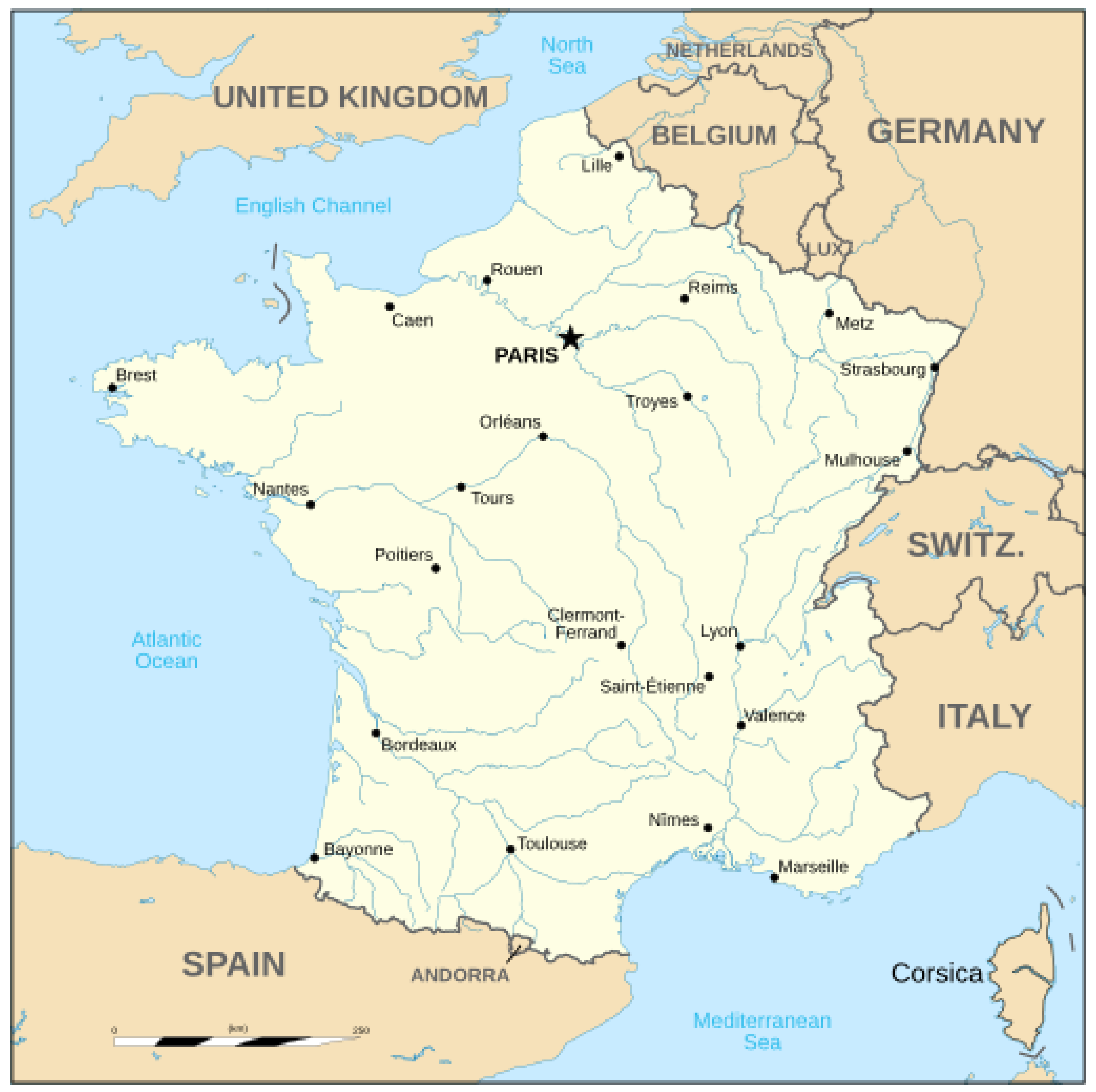
3. Data and Study Site
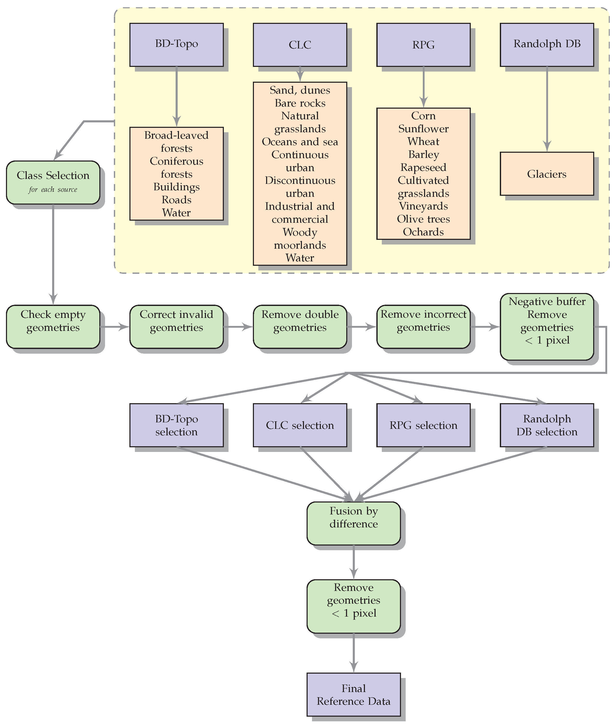
The experiments presented in this paper are carried on the complete metropolitan (European territory), continental (without Corsica) France, see Figure 1, which amounts to 535,000 km 2 . The climate is mainly oceanic—Cfb, Cwb and Cfc in the Köppen classification [28]—with a smaller part close to the Mediterranean Sea belonging to the Csa and Csb categories.

3.1. Reference Data

Reference data for the land cover classes are used for supervised classifier training and validation. Operational land cover map production over large areas cannot rely on field campaigns because huge amounts of costly data would need to be collected, most importantly jeopardising the timeliness of the land cover map. The choice made in this work is to rely on existing databases to build the reference data sets needed for the supervised classification and the subsequent validation of the land cover maps. These data sources will contain fatal errors due to changes in the landscape. The choice here is to rely on the classification algorithm to overcome these issues. Four data sources have been used in order to build a unique reference data set:
  • Corine Land Cover (CLC) 2012 [29].
  • French National Geographic Institute “BD Topo” [30].
  • The agricultural Land Parcel Information System “Registre Parcellaire Graphique” (RPG) [31].
  • The Randolph Glacier Inventory [32].
These data sources were combined to build the following land cover nomenclature:

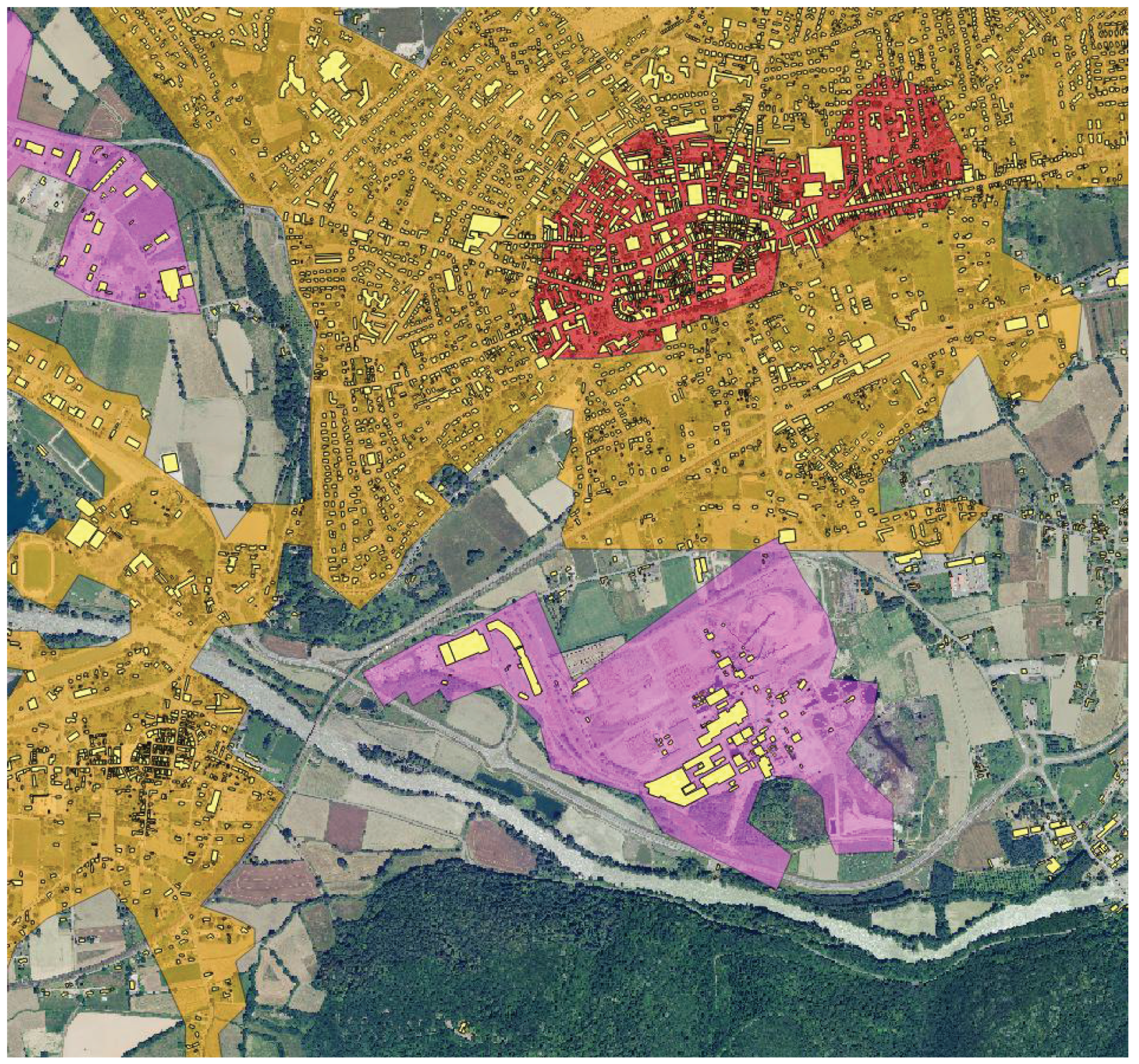
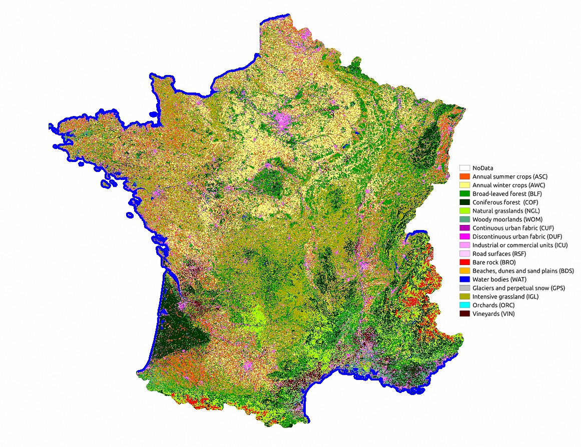
3.1.1. Artificial Areas

  • CUF Continuous urban fabric (CLC 111): Most of the land is covered by structures and the transport network. Building, roads and artificially surfaced areas cover more than 80% of the total surface. Non-linear areas of vegetation and bare soil are exceptional.
  • DUF Discontinuous urban fabric (CLC 112): Most of the land is covered by structures. Building, roads and artificially surfaced areas associated with vegetated areas and bare soil, which occupy discontinuous but significant surfaces.
  • ICU Industrial or commercial units (CLC 121): Artificially surfaced areas (with concrete, asphalt, tarmacadam, or stabilised, e.g., beaten earth) without vegetation occupy most of the area, which also contain buildings and/or vegetation.
  • RSF Road surfaces (BD Topo): motorway rest areas, parking areas, motorway networks, larger than 50 m.

3.1.2. Agricultural Areas

  • Arable land
    • ASC Annual summer crops (RPG): annual crops which are seeded from March to mid June and harvested at the end of the summer (mid August to mid September); these are mainly corn and sunflower.
    • AWC Annual winter crops (RPG): annual crops which are seeded between November and February and harvested at the beginning of the summer (mid June to the end of July); these are mainly wheat, barley and rapeseed.
    • IGL Intensive grassland (RPG): dense grass cover, of floral composition, not under a rotation system.
  • Perennial crops
    • ORC Orchards (RPG): parcels planted with fruit trees or shrubs.
    • VIN Vineyards (RPG): areas planted with vines.

3.1.3. Forest and Semi-Natural Areas

  • Forests
    • BLF Broad-leaved forest (BD Topo).
    • COF Coniferous forest (BD Topo).
  • Shrubs and herbaceous vegetation
    • NGL Natural grasslands (CLC 321): low productivity grassland; often situated in areas of rough, uneven ground and frequently includes rocky areas, briars and heathland.
    • WOM Woody moorlands (BD Topo): spontaneous vegetation dominated by woody plants (heather, briar, broom, etc.) and semi-woody plants (fern, phragmites, etc.) shorter than 5 m.
  • Open spaces with little or no vegetation
    • BDS Beaches, dunes and sand plains (CLC 331): beaches, dunes and expanses of sand or pebbles in coastal or continental locations, including beds of stream channels with torrential regime.
    • BRO Bare rock (CLC 332): Scree, cliffs, rock outcrops, including active erosion, rocks and reef flats situated above the high-water mark.
    • GPS Glaciers and perpetual snow (Randolph): land covered by glaciers or permanent snowfields.
    • WAT Water bodies (CLC 523 and BD Topo): all water bodies longer than 20 m and all water courses larger than 7.5 m.
Note that some classes coming from different data sources could lead to some overlap between categories. Since the classes should be mutually exclusive, the intersections were removed. More details on the procedure implemented for the fusion of the different data sources are given in Section 4.2.

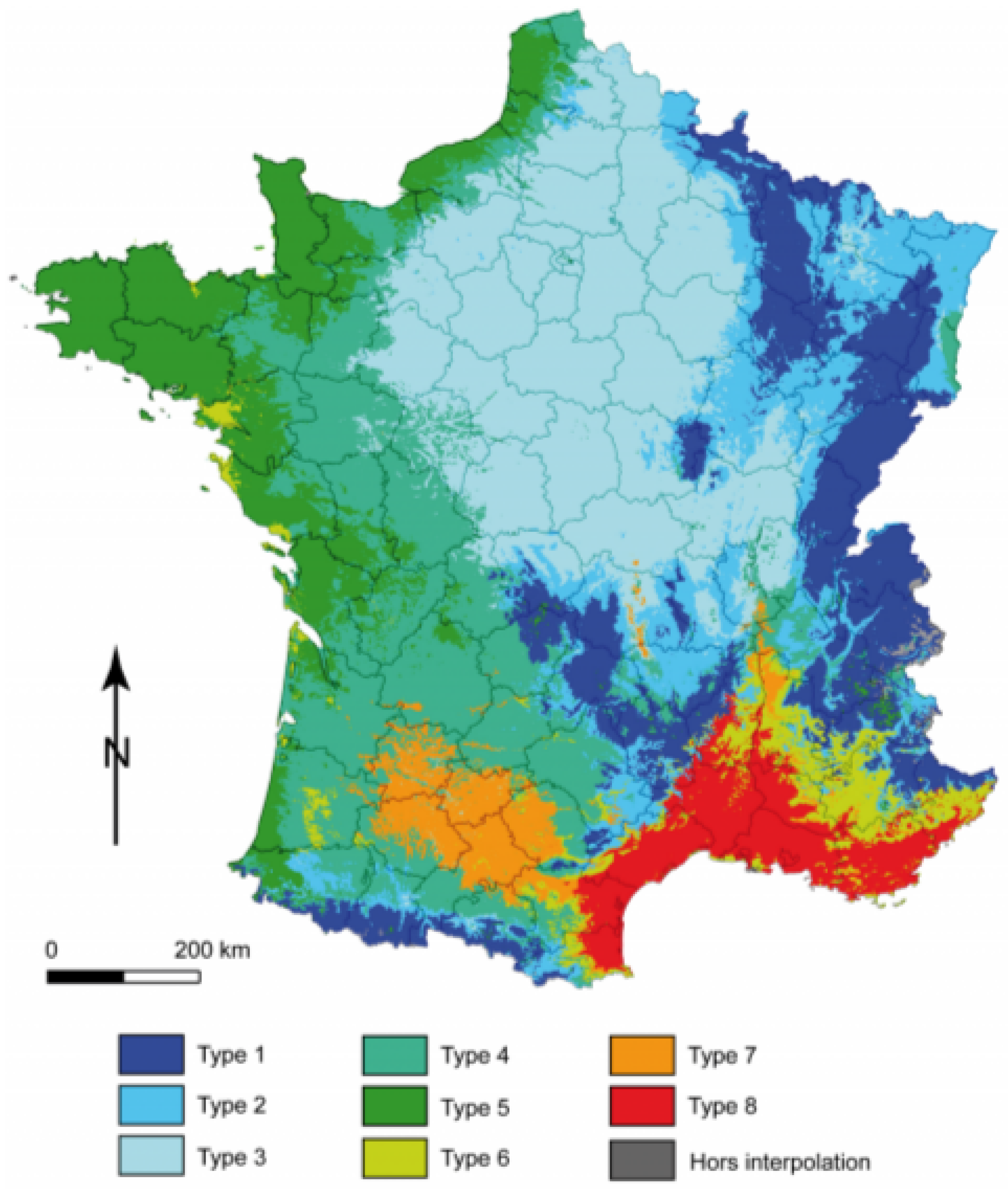
3.2. Climatic Stratification

Although not used as training nor validation data, a map of climatic regions is used for stratification for one of the presented land cover approaches (see Section 4.4.3). This map was originally published in [33] and divides the area of study in 8 disjoint climatic regions (Figure 2). The original map was slightly modified in order to eliminate very small regions (smaller than 100 km 2 ).

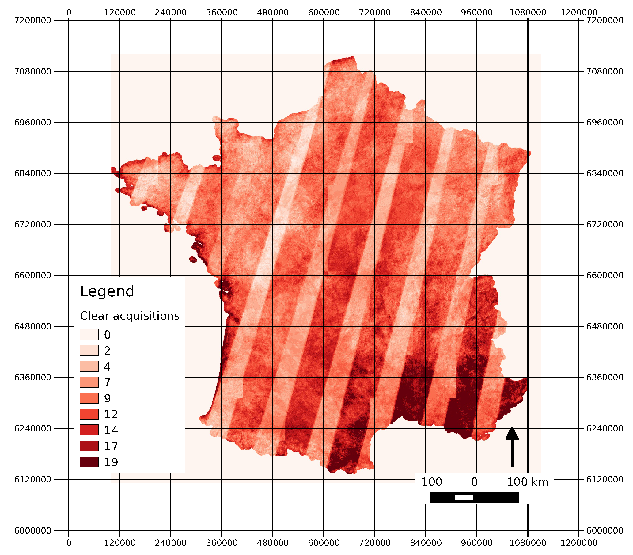
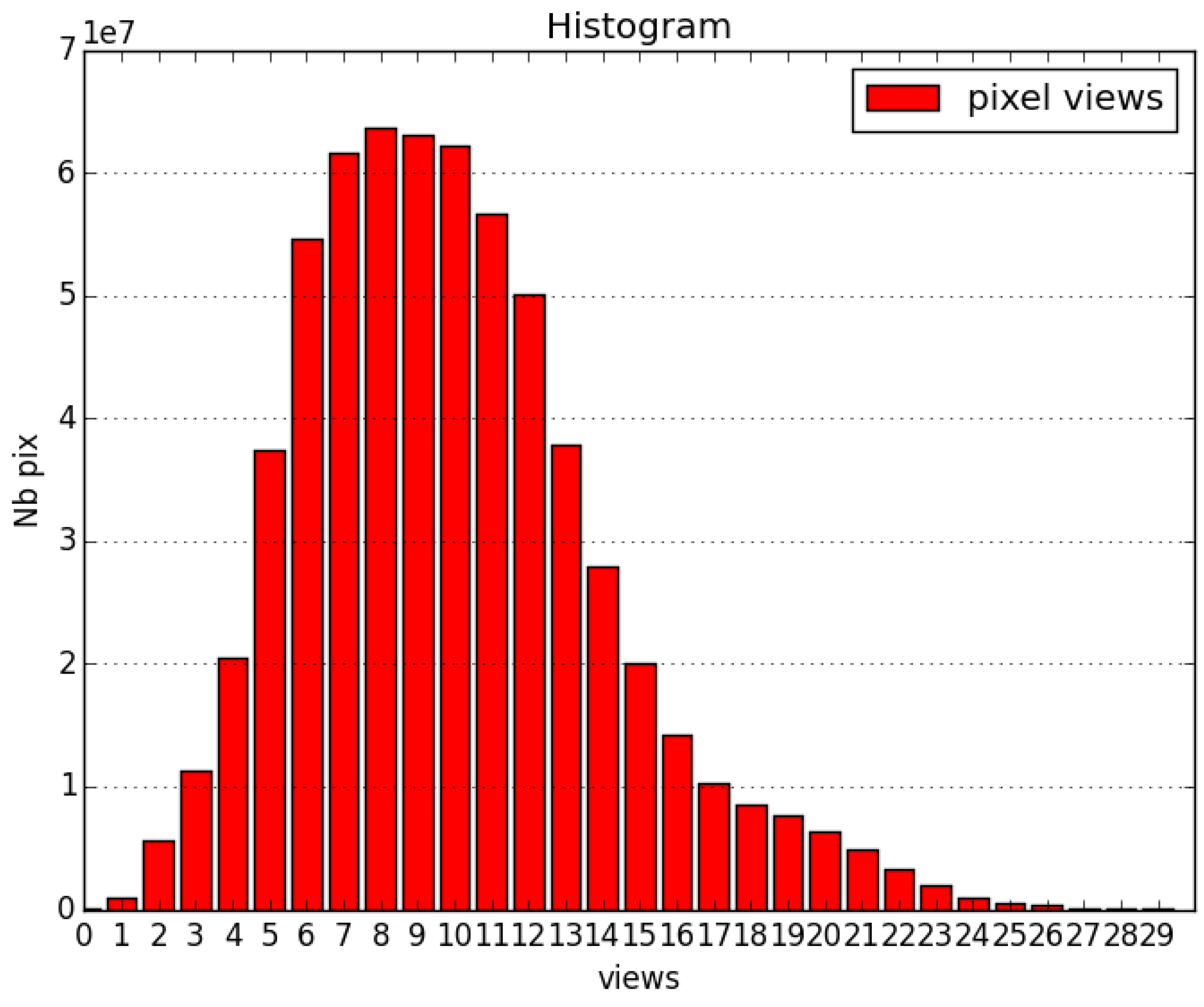
3.3. Satellite Imagery
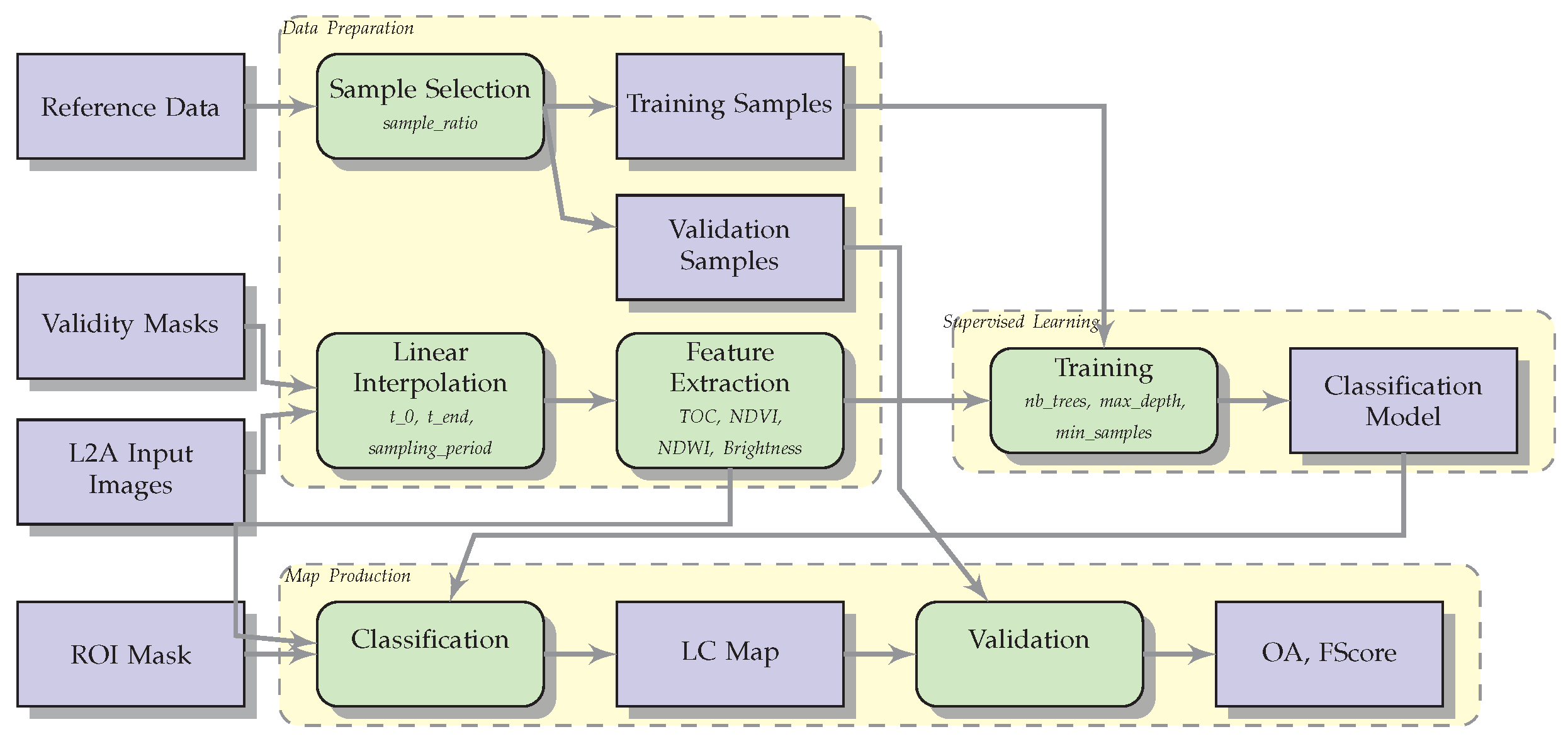
Landsat-8 [6] was the only source of image data used in this work. All Level 2A data available through the Theia Land Data Centre (http://www.theia-land.fr/en/presentation/products) over the study area for the year 2014 were used. The Landsat products are orthorectified prior to their release by the USGS and then, Theia processing chains based on the algorithms described in [34] perform cloud (and cloud shadow) screening and atmospheric corrections. This amounts to 740 Landsat acquisitions over 54 path-rows, which correspond to an average of 13.7 dates per scene. The complete list of images used is given in Table 1. However, as it will be described in Section 4.3.1 due to cloud cover and satellite swath overlap, the effective number of times that a pixel contains valid surface reflectance values can range from 0 to 29.

4. Methodology

4.1. Introduction

The proposed approach is based on a classical supervised classification procedure. The main originality of the procedure is to make this approach usable over very large territories, dealing with huge volumes of data and allowing fully automatic (no human operator) land cover map production in very short production times. The approach is also meant to be generic, that is, independent of the class nomenclature and the landscape. Figure 3 shows the block diagram for the kernel of the processing chain. The inputs to the procedure are:
  • A reference data with labelled samples (geographical positions for which the land cover class is known).
  • Image time series processed to level 2A (ortho-rectified, surface reflectances).
  • Validity masks for the image time series: for each date in the time series every pixel is flagged valid (surface reflectance) or invalid (cloud, cloud shadow, saturation, out of satellite swath).
  • As optional input, a region of interest (ROI) mask can be provided to eliminate areas where the map generation is not wanted.
The reference data is split into training and validation subsets (see Section 4.2 for details). The image data is pre-processed in order to ensure spatial and temporal homogeneity, as described in Section 4.3.1 and then image features for the classification are extracted (see Section 4.3.2). After that, classifier training and image classification are performed. These 2 steps can be implemented using different techniques in order to deal with landscape variability across large areas and reference data availability as described in Section 4.4. This is one of the main contributions of this work which makes the whole procedure possible. Finally, once the land cover map has been produced, a standard set of performance measures are computed for the validation of the map.
This processing work-flow has been implemented into the iota2 processing chain which is available as free software [35]. The software makes extensive use of the Orfeo Toolbox remote sensing image processing library [36,37] version 5.4 [38] and needs the Temporal Gapfilling [39] and Vector Tools [40] libraries. The iota2 processing chain runs on any POSIX operating system. It makes extensive use of parallel processing and can run both on shared memory multi-core machines and high performance computing clusters with hundreds of nodes. On a 120 node cluster, the land cover maps presented in Section 5, which use all available Landsat-8 images during one year over France, are produced in less than 12 h.

4.2. Reference Data Preparation

As introduced in Section 3.1, the reference data used for classifier training and map validation have different origins, thus data cleansing and harmonisation are required. A set of processing steps have been designed and implemented in a free software library [40] so that the process is streamlined, automatic and reproducible.
There are 2 main steps in the procedure (see Figure 4): cleansing each data source and their fusion. The cleansing step starts by selecting, from each data source, the polygons corresponding to the classes of interest. The databases from which each class is extracted are indicated in Section 3.1 and in Figure 4. The data cleansing comprises the following sequence of steps:
  • elimination of empty entities;
  • correction of invalid geometries, as for instance closing polygons;
  • elimination of duplicated entities;
  • elimination of invalid geometries which can not be corrected;
  • optional negative buffering (erosion of polygons to eliminate object boundaries which often correspond to mixed pixels);
  • elimination of polygons smaller than a minimum area (typically, the size of a pixel).
Once each data source has been prepared, they can be merged in order to build the final reference data set. The fusion work-flow mainly consists in pairwise checking the data sources for polygon overlaps. A symmetric difference is computed in order to eliminate intersections, since they correspond to areas for which different sources indicate different land cover classes. This kind of mismatch is rare, but may exist due to different class definitions between the data providers or errors in the data sources. Since this step can reduce the size of the polygons, the elimination of small polygons has to be applied again at the end of the processing. An additional refinement step can be applied for some classes. Sometimes, different reference data sources can complement each other for the characterisation of a particular land cover class. For instance the “Discontinuous Urban Fabric” class from CLC may contain large patches of vegetation. Although this is compliant with the CLC minimum mapping unit, it can be a problem for the production of high resolution land cover maps. On the other hand, the BD Topo does not provide the semantics of “continuous” or “discontinuous” for urban areas, but provides instead the individual buildings. These 2 data sources can be combined in order to obtain a reference data set with CLC semantics, but with fewer outliers.
Figure 5 shows individual buildings given by BD Topo and CLC polygons for “Continuous Urban Fabric” (red), “Discontinuous Urban Fabric” (orange) and “Industrial and Commercial Units” (pink). By applying a set of buffering operations to the individual buildings followed by an intersection with the CLC polygons, a refined reference data set can be obtained as illustrated in Figure 6.
This kind of processing is completely generic, and allows to merge data sources in order to keep the semantics of one and the geometric quality of the other. Although the final result is not perfect, it strongly reduces the number of mislabelled samples. In the case of the proposed approach, the choice of a classifier robust to label noise has been made, which allows to tolerate more than 15% of mislabelled samples in the training step.
After the generation of the reference data set as described above, the data is split into 2 disjoint sets for classifier training and land cover map validation respectively. The samples are split at the polygon level and not at the pixel level. This ensures that pixels from the same polygon, which could be very similar, are not used for training and validation, because this would yield optimistic values for the quality metrics described in Section 4.5.1.
The processing chain allows also to perform N different splits of the reference data, which can be used to perform N independent trainings and validations in order to properly estimate confidence intervals for the quality metrics.

4.3. Image Pre-Processing

4.3.1. Temporal Gapfilling and Resampling

For the proposed approach to be fully automatic and without the need for adaptation to different areas or different map nomenclatures, no rules or strategies tailored to a particular land cover class or landscape can be used. Therefore, no date selection in terms of season or vegetation phenology is used and the use of all available image data is proposed here.
In order to cover a very large territory, several satellite tracks (orbits or paths) are needed. Therefore, even if the used satellite has a constant revisit period, the acquisition dates for adjacent tracks are different. Figure 7 illustrates the Landsat-8 cover of France. Each North-South sequence of acquisitions has the same dates with a revisit cycle of 16 days. Adjacent tracks are acquired 8 days apart with an overlap area.
In the proposed procedure, each pixel will be characterised by a time series of image features (surface reflectances and spectral indices, see Section 4.3.2 for the details). Therefore, the fact that different pixels may have different acquisition dates, will cause issues.
Another source of inhomogeneity of temporal sampling is the presence of clouds and cloud shadows. Cloud presence has great variability in terms of location and season. Figure 8 displays the map of the count of clear pixels (no cloud, no shadow, no saturation) for the study area. The count goes from 2 to 29 for the whole 2014 year (Figure 9). The effect of climatic areas and satellite track overlap is clearly visible.
The Landsat-8 Level 2A data produced by the Theia Land Data Center is distributed as tiles of 110 km × 110 km with a 10 km overlap (see Figure 10). The tile is the unit of processing for the atmospheric corrections. Only tiles with less than 90% cloud cover are processed by Theia, therefore, a Landsat scene can be only partially processed depending on the cloud cover fraction on each of the intersecting tiles. The effect of this procedure is visible, for instance in the South-Eastern part of Figure 8.
All these sources of irregularity in acquisition dates indicate that some data cleansing has to take place before the classification is implemented.
The same approach used in [7], which consists of a linear interpolation of the invalid pixels using the previous and following cloud-free dates, was used here. The interpolation is applied over surface reflectance values and before the computation of derived spectral indices. The use of interpolation allows to estimate the values of the surface reflectances for any date, not only the dates of the invalid pixels. This allows the choice of a set of common dates for all the pixels of the area which in turn solves the issue of temporal shifts between adjacent satellite tracks. At the end of the gapfilling and resampling, the same set of virtual acquisition dates is used for all the pixels of the area. These dates are computed by using the first available date as the starting point and setting a temporal period of 16 days (the revisit cycle of Landsat-8).

4.3.2. Feature Extraction

After temporal gapfilling and resampling, the feature vector that will be used for the classification of each pixel is built. For every date 3 spectral indices are computed:
  • the NDVI [41] to highlight vegetation cover;
  • the NDWI [42] to enhance water and wet areas;
  • the brightness (defined as the Euclidean norm of the surface reflectances).
Therefore, each pixel is characterised by the regularly sampled time profiles of the surface reflectances and the 3 spectral indices, which amounts to 198 features: 6 spectral bands plus 3 radiometric indices on 22 dates.

4.4. Classification

4.4.1. Classifier Choice and General Work-Flow

As explained in previous sections, the reference data used for the classification is built from data sources which may not be up to date. Although techniques for outlier detection could be implemented, the choice made in this work is to rely on the fact that a classifier which avoids over-fitting will be robust to this kind of errors. Random forests (RF) [43] are known to be robust to label noise [44,45] and have been chosen in our approach. RF are state-of-the-art in remote sensing image processing and yield classification accuracies as high as more sophisticated algorithms as for instance support vector machines, but with a much lower computational complexity. They are also stable with respect to the choice of parameters [46] which makes them excellent candidates for operational processing chains. The RF implementation used here is the one provided by OpenCV 2.11 which is available through the supervised classification framework of Orfeo Toolbox 5.4 [38].
The choice of parameters for the RF classifier is not very sensitive for this kind of problem as demonstrated in [46], and 100 trees, a maximum depth for each tree of 25 levels and a minimum number of 5 samples per node have been used. The number of features randomly selected at each node equals the square root of the total number of features.
This allows the implementation of the kernel of the processing chain as described in Figure 3. Therefore, a single classifier using all reference data and available images could be trained and applied over the whole study area. However, this would need a very large amount of (shared) memory. Thus, a tile-based approach which is able to train several classifiers over different areas has been implemented as described in Section 4.4.2. The possibility of training and applying different classifiers over different areas gives also the possibility of performing spatial stratification. This second approach is described in Section 4.4.3.

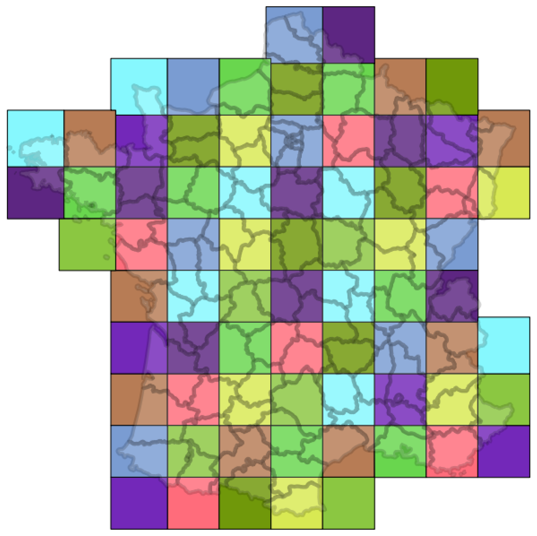
4.4.2. Tile-Based Approach

In order to train a single classifier over the whole area, a huge amount of RAM would be needed. Since RF decision function is the majority vote of a committee of decorrelated decision trees, one can train several RF over different subsets of the training set and combine the results of each individual RF without much modification of the final result. The processing chain allows to perform the training of several classifiers using data coming from a subset of the tiles. These subsets can be disjoint, comprise common tiles or contain all the tiles, which would result in the trivial case of a single classifier. Once the classifiers are trained, the classification step can implement 2 strategies:
  • each tile is classified using the classifier trained with the same tile;
  • each tile is classified using all the classifiers and a majority vote used for the final decision.
The choice of the subset of tiles used for classifier training is important. A different classifier per tile could be used or a classifier per group of adjacent tiles. Although not reported here for the sake of brevity, the choice of disjoint classifiers trained over randomly selected tiles, followed by a majority voting of all classifiers gives a good trade-off between complexity and accuracy. Therefore, this is the approach that will be evaluated in the remainder of this paper. Figure 11 shows an example of tile distribution. Each colour identifies the subset of tiles for which a common classifier is trained.

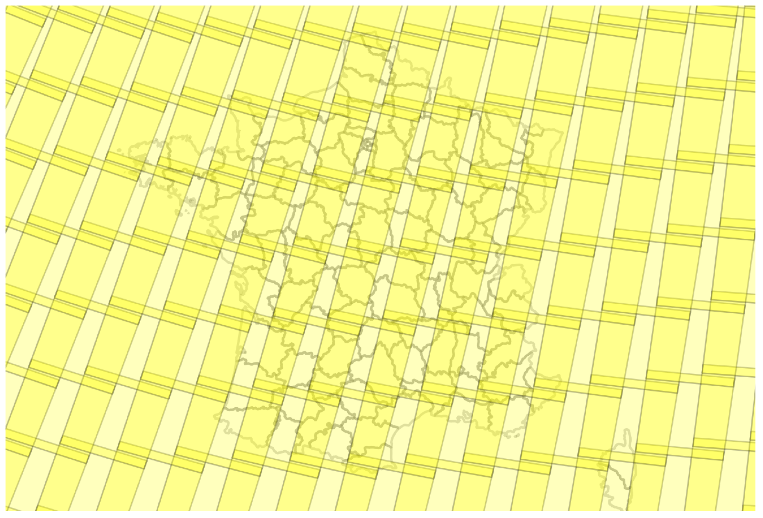
4.4.3. Spatial Stratification

One of the main difficulties in the production of land cover maps over very large areas is the intra-class variability. Indeed, the same semantic category can have different spectral and temporal signatures depending on the areas. On the other hand, some classes are only present in certain areas, which means they are a minority over the complete area and they can therefore be difficult to account for by a classifier that is designed to maximise the overall accuracy, and therefore giving more weight to majority classes.
Although partitioning classifiers such as RF, which are based on decision trees, tend to build subclasses automatically, supplying additional information to the classifier by identifying for instance climatic areas can be useful. In this work, we have used the eco-climatic map presented in Section 3.2 published by [33] and illustrated in Figure 2. This map can be used in order to divide the area to be mapped into different strata that will be processed independently.
In terms of implementation of the classification, there is no major difference with respect to the tiled approach. The intersection of the tile footprints and the eco-climatic areas is used to define the disjoint regions on which independent classifiers are trained. Then each region is classified using only the classifier trained over this region. In the case of very large regions for which the memory optimisations described in Section 4.4.2 would be needed, the training data set is split into smaller subsets and the majority vote strategy of the tile-based approach is used.

4.5. Land Cover Map Validation

In order to assess the quality of the produced land cover maps, several approaches can be used. The classical set of indices derived from the confusion matrix will be used as described in Section 4.5.1. These are global statistics which give summarised information. However, it may sometimes be useful for the users to assess the quality of the map locally in a given area. For this purposes, a map indicating the confidence of the classifier on the decision for each pixel of the land cover map can be provided as described in Section 4.5.2. Finally, a visual inspection in order to highlight anomalous patterns will also be presented in Section 5.3.

4.5.1. Confusion Matrix and Derived Indices

The confusion matrix (also known as contingency table) is a double entry table where row entries are the actual classes (reference data) and column entries are the predicted classes (output of the classifier). Each cell of the table contains the number of elements (pixels in pixel-based classification) of the row class predicted by the classifier as belonging to the column class.
The diagonal elements in the matrix represent the number of correctly classified pixels of each class, i.e., the number of ground truth pixels with a certain class label that are actually classified with the same class label during classification. The off-diagonal elements represent mis-classified pixels or the classification errors, i.e., the number of ground truth pixels that ended up in another class during classification. Off-diagonal row elements represent ground truth pixels of a certain class which were excluded from that class during classification. Such errors are also known as errors of omission or exclusion. Off-diagonal column elements represent ground truth pixels of other classes that were included in a certain classification class. Such errors are also known as errors of commission or inclusion. The Overall Accuracy (OA) is the sum of the diagonal elements divided by the sum of all elements of the confusion matrix.

Producer’s Accuracy

Accuracy (also known as producer’s accuracy or recall): it is the fraction of correctly classified pixels with regard to all pixels of that ground truth class. For each class of ground truth pixels (row), the number of correctly classified pixels is divided by the total number of ground truth or test pixels of that class.
P A i = j = 1 r n i i n i j ,
where r is the number of classes and n i j is the element of the confusion matrix in row j and column i, that is, the count of elements of class j classified as class i. The average accuracy is calculated as the sum of the per class accuracies divided by the number of classes in the test set.
P A = 1 r i = 1 r P A i

User’s Accuracy

Reliability (also known as user’s accuracy or precision): it is the fraction of correctly classified pixels with regard to all pixels classified as this class in the classified image. For each class in the classified image (column), the number of correctly classified pixels is divided by the total number of pixels which were classified as this class.
U A i = j = 1 r n i i n j i
The average reliability is calculated as the sum of the per class reliabilities divided by the number of classes in the test set.
U A = 1 r i = 1 r U A i
Sometimes it is useful to measure an average relative precision, which is computed over a confusion matrix where the rows are normalised in order to give the same weight to all classes. This allows to avoid biases in the precision when a class has more validation samples than the others.

FScore

The FScore (also known as F-1 score or F-measure) is the harmonic mean of UA and PA, and reaches its best value at 1 and worst score at 0.
F S c o r e = 2 × U A × P A U A + P A
It can be computed per class or for the whole map. Also, as the precision, the relative FScore can be computed using the relative precision.

Kappa Coefficient

Since part of the agreement between the classifier’s output and the reference data can be due to chance, the metrics presented above may be optimistic. The Kappa coefficient (κ) expresses a relative difference between the observed agreement P o and the random agreement which can be expected if the classifier was random, P e .
κ = P o P e 1 P e
where P o = 1 n i = 1 r n i i is the agreement and P e = 1 n 2 i = 1 r n i . n . i
κ is a real number between −1 and 1 and can be interpreted as follows:
Agreementκ
Excellent>0.81
Good0.80–0.61
Moderate0.60–0.41
Weak0.40–0.21
Bad0.20–0.0
Very bad< 0

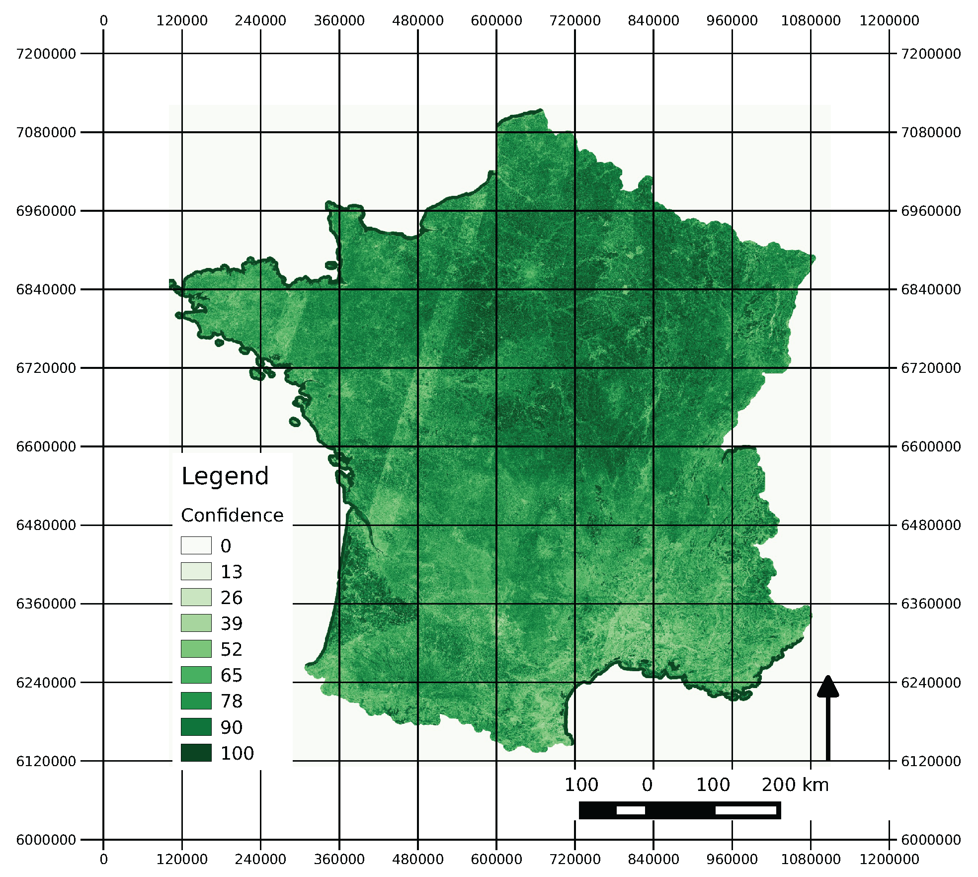
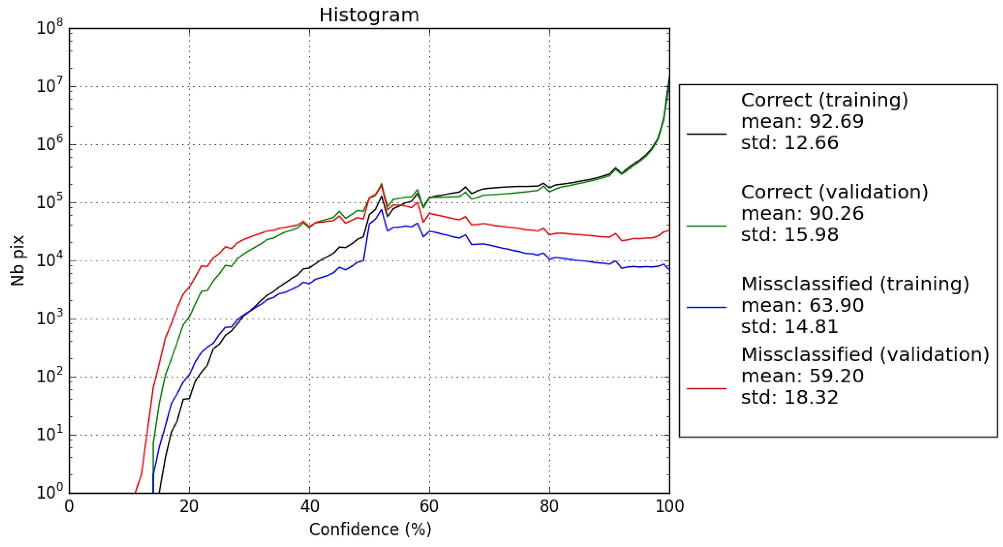
4.5.2. Confidence Map
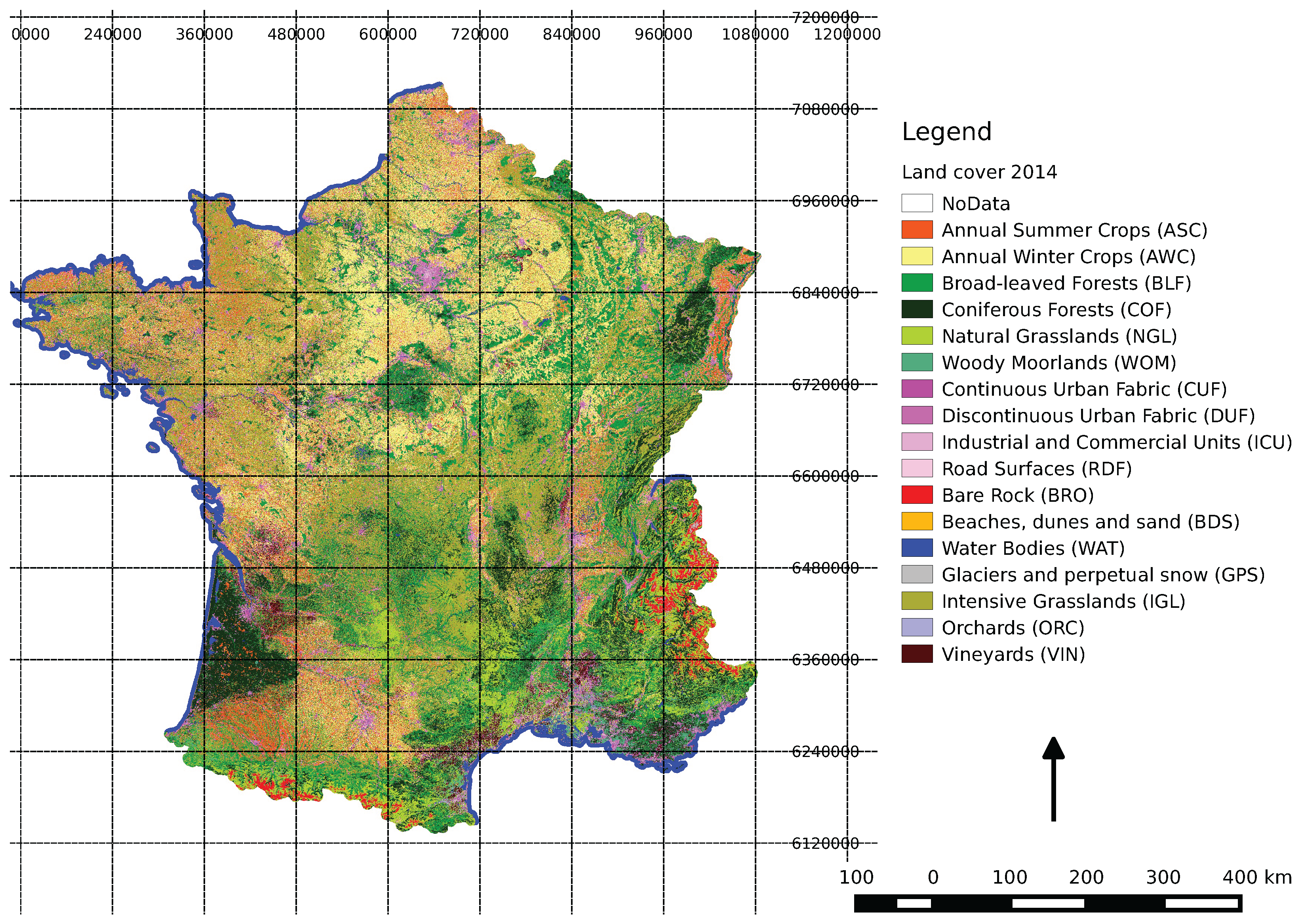
The land cover map contains for each pixel the label selected by the decision function implemented by the classifier. However, information on how confident the decision of the classifier is can help users to better use the produced map. The RF decision function is a majority voting over the labels selected by the set of decision trees in the forest. It is therefore possible to estimate a confidence by using the distribution of the labels produced by each tree [47]. The probability of each class can be estimated as the proportion of trees in the forest that have chosen this label. One can therefore estimate a confidence in the decision by using the probability of the majority class. Another measure usually used is the so-called margin, which is the difference between the 2 highest probabilities. The former will be used in this work. In the case of majority voting for fusing the results of several classifiers (as in the tile-based approach or in large eco-climatic regions) the confidence is computed from the confidence of each of the N voting classifier as follows:
C = i = 1 N L i = L m a x c i + 1 L i L m a x c i N ,
that is, the average of the confidences c i for the classifiers choosing the majority label L m a x plus the average of 1 minus the confidences of the classifiers choosing a different label. Although this confidence estimation can be valuable for the map user, one has to bear in mind that it is an estimation of the classifier itself, and therefore it may be wrong. The correlation between the confidence and the classification quality will be assessed in Section 5.2.

5. Results

In this section we analyse the performances of the land cover map production system presented in Section 4 and we compare the tile-based approach with the stratified one (the map is shown in Figure 12). The quality of the maps produced is evaluated quantitatively using the well known metrics presented in Section 4.5.1. A visual assessment of the maps is also proposed to highlight some kinds of errors which can not be detected in the overall statistical evaluation.

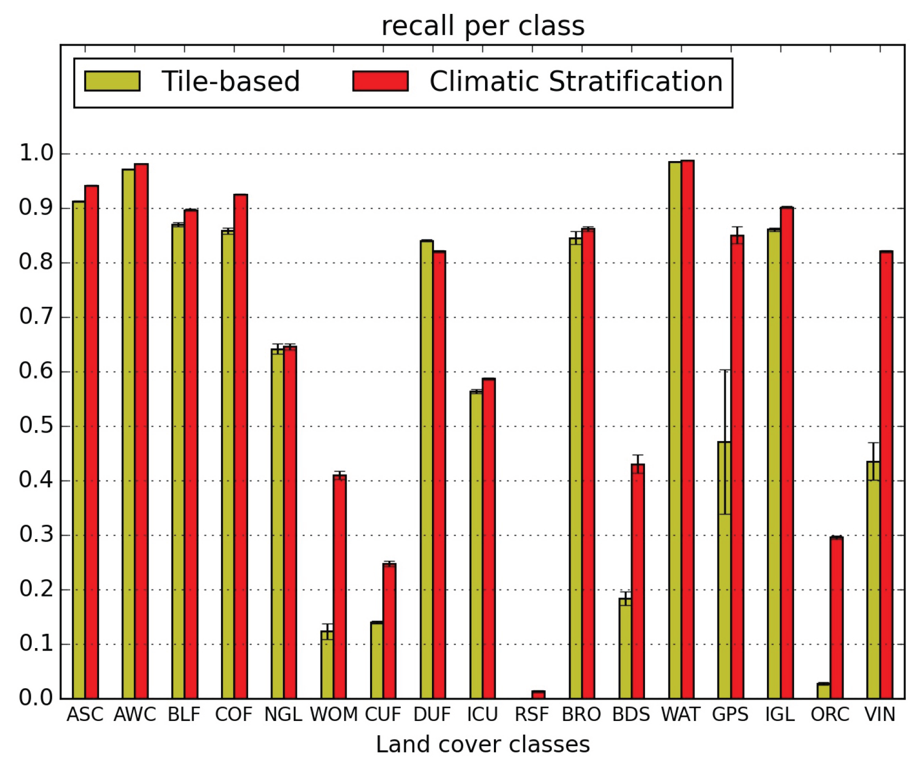
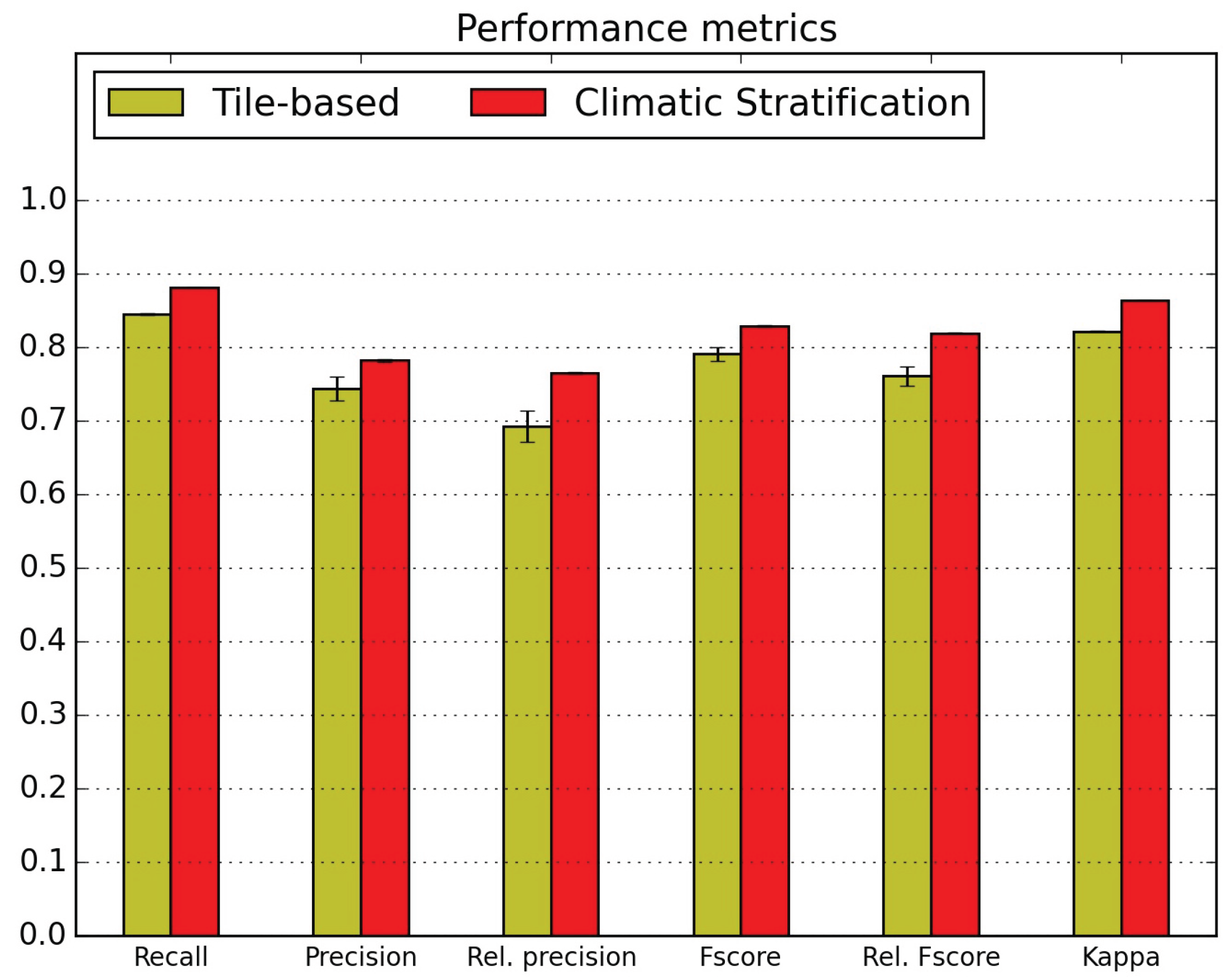
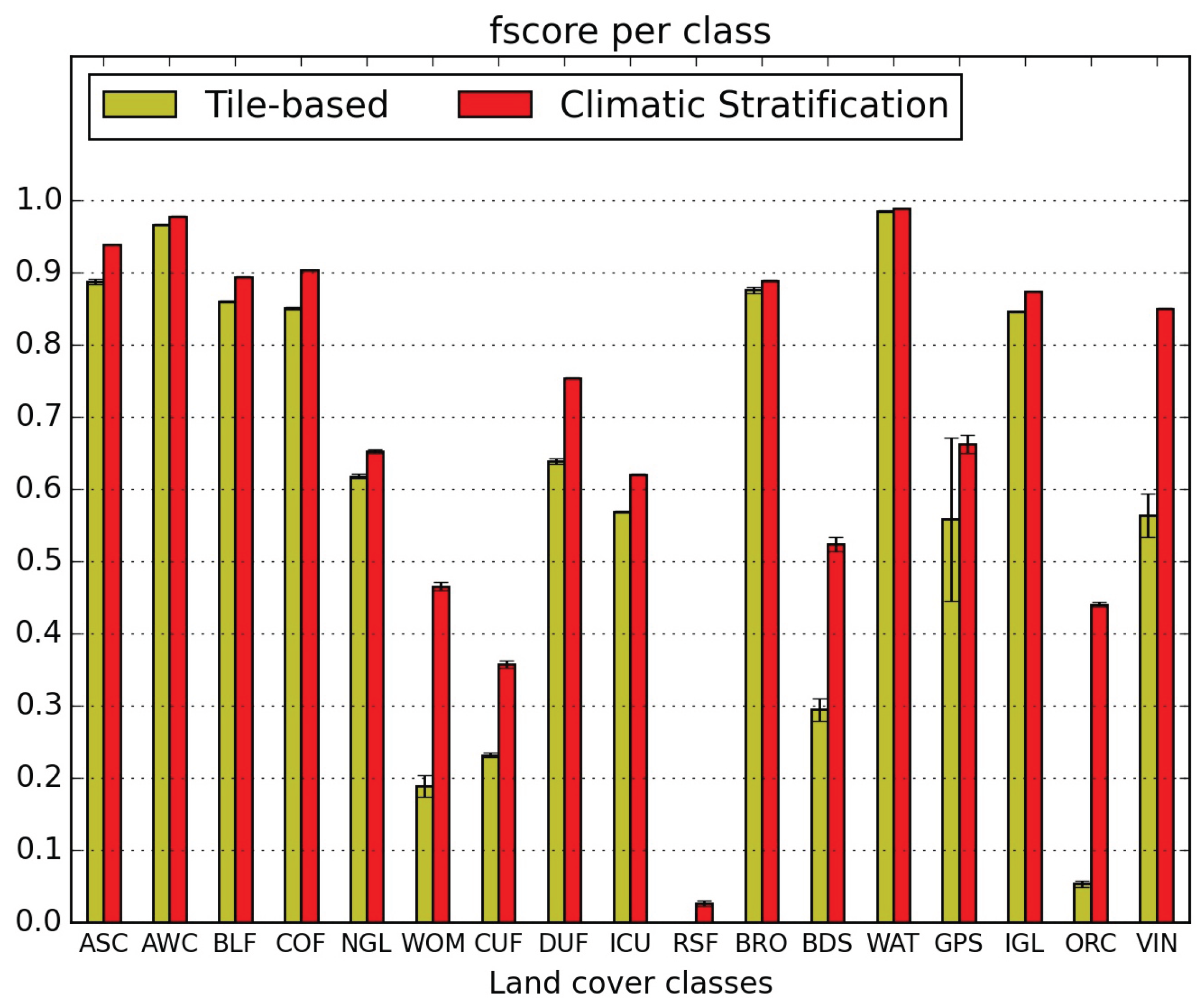
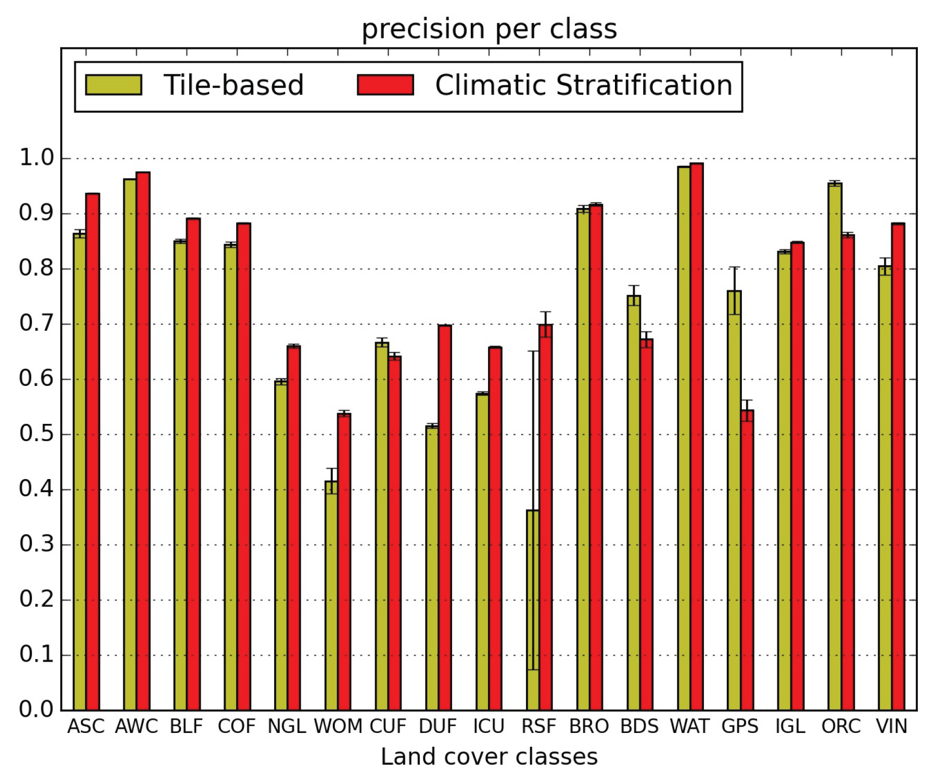
5.1. Quantitative Map Evaluation

Figure 13 presents the set of global metrics for the 2 mapping modes (tile-based in yellow and stratified in red). The average metrics over 10 runs using different training and validation sets (of about 26 million pixels each) are displayed, together with the 95% confidence intervals. The performances are very good with κ coefficients above 0.8 (0.82 for the tile-based approach and 0.86 for the climatic stratification) and recalls above 0.84 (0.84 for the tile-based approach and 0.88 for the climatic stratification). One can observe that the eco-climatic stratification yields better results for all the metrics. It can also be noted that the confidence intervals for the metrics are very narrow (the results are statistically significant since the 95% confidence intervals do not overlap) and they are narrower when stratification is used.
Figure 14 displays the FScore values per class, which shows that the stratification improves the results for all classes, but even more for those classes which have fewer training samples (woody moorlands, beaches and dunes, orchards and vineyards). The class woody moorlands is much better recognised using stratification, mainly because of its heterogeneity across climatic regions. The class glaciers and perpetual snow is spread over mineral surfaces and water bodies when the stratification is not used.
Figure 15 and Figure 16 present the recall and the precision per class. They show that the improvement in performances for these minority classes in the case of the stratification, comes from the recall, which was lower and with wider confidence intervals in the tile-based mode.
Table 2 and Table 3 show the confusion matrices for the tile-based approach and the eco-climatic stratification respectively. They allow the detailed pairwise analysis of the errors for both approaches. Several aspects of the improvement yielded by the eco-climatic stratification can be highlighted:
  • the confusions between natural grasslands (NGL) and woody moorlands (WOM) are reduced in both directions, as well as the WOM classified as discontinuous urban fabric (DUF);
  • orchards (ORC) classification is very much improved (they were nearly not detected without stratification) but they are still confused with intensive grasslands (IGL); however the two other main confusions, with broad leaved forests (BLF) and DUF, are very much reduced;
  • similarly, vineyards (VIN) which were mainly mis-classified as annual summer crops (ASC) and DUF are reduced to less than 5%;
  • the confusion of glaciers and perpetual snow (GPS) with bare rock (BRO) is divided by 3;
  • the confusion of beaches dunes and sand (BDS) with industrial and commercial units (ICU) is reduced from 33% to 8%, but the confusion with water (WAT) increases from 17% to 21%.
Another minor quantitative improvement, but which is important from the thematic point of view is the reduction of IGL classified as NGL (from nearly 8% to less than 5%). Also, NGL mis-classified as DUF are reduced from nearly 8% to 1.4% The 4 urban classes are sligthly improved but the confusions between them remain.

5.2. Use of the Confidence Map

Figure 17 shows the confidence map obtained for the land-cover map of Figure 12 where the darker the pixel, the higher the confidence. One can observe that confidence is influenced by the number of dates for which every pixel is valid (some of the patterns of Figure 8 are observed), but also by the class. For instance, the Landes forest in the south-western part is easily recognised in the confidence map.
Since confidence values are computed by the classifier, one can argue that they may not be reliable in the case of a miss-classification. It is therefore interesting to study how confidence values are related to correct and incorrect classifications. Also, confidence values can have different distributions for pixels having been used for the training of the classifier, compared with pixels not used for the learning step.
Figure 18 presents the histograms of the confidence values for 4 categories of samples:
  • training samples correctly classified (black);
  • validation samples correctly classified (green);
  • mis-classified training samples (blue);
  • mis-classified validation samples (red).
For confidence values lower than 50%, training and validation pixels have different behaviours. This does not allow to use confidence values to make any inference about the correctness of the label given by the classifier in this case. Training and validation pixels have similar confidence distributions for confidence values higher than 50%. The histograms show that correctly classified (training or validation) samples have a higher probability of having confidences higher than 60%. For confidence values higher than 80%, a pixel has more than 20 times more chances of being correctly than incorrectly classified. Therefore, this type of map can be very useful for the interpretation of the land cover map.

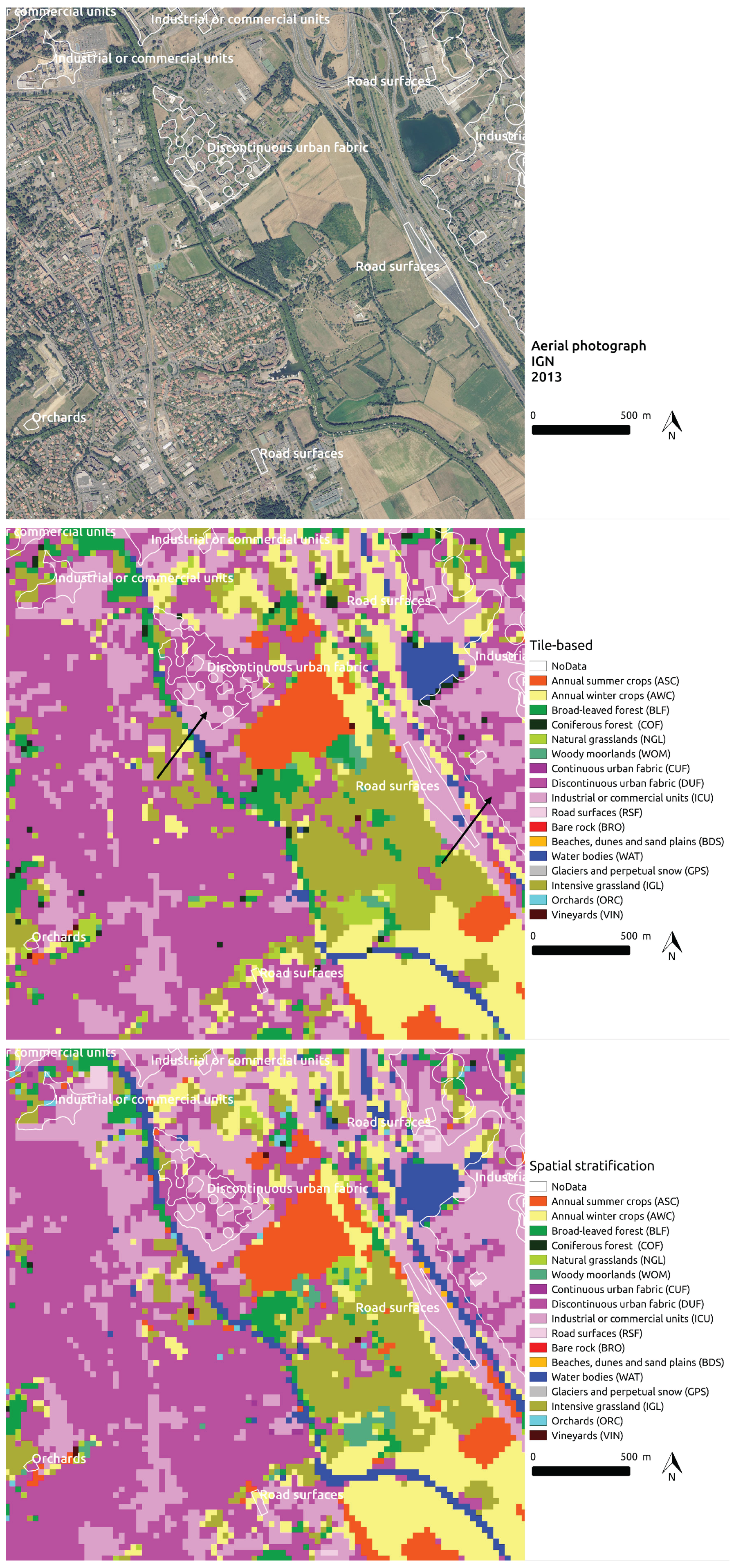
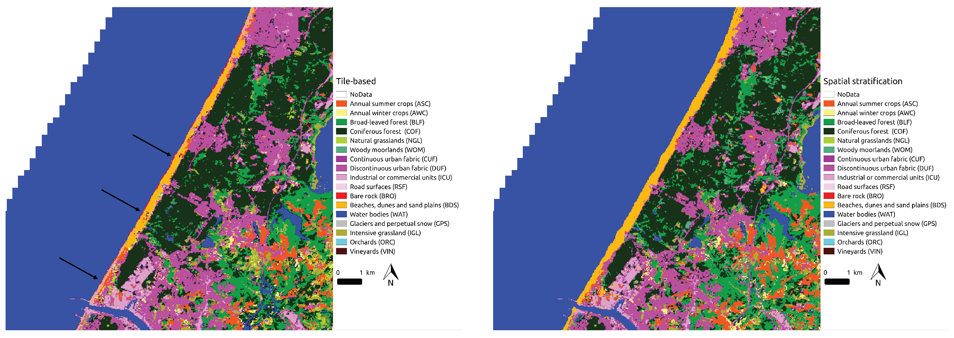
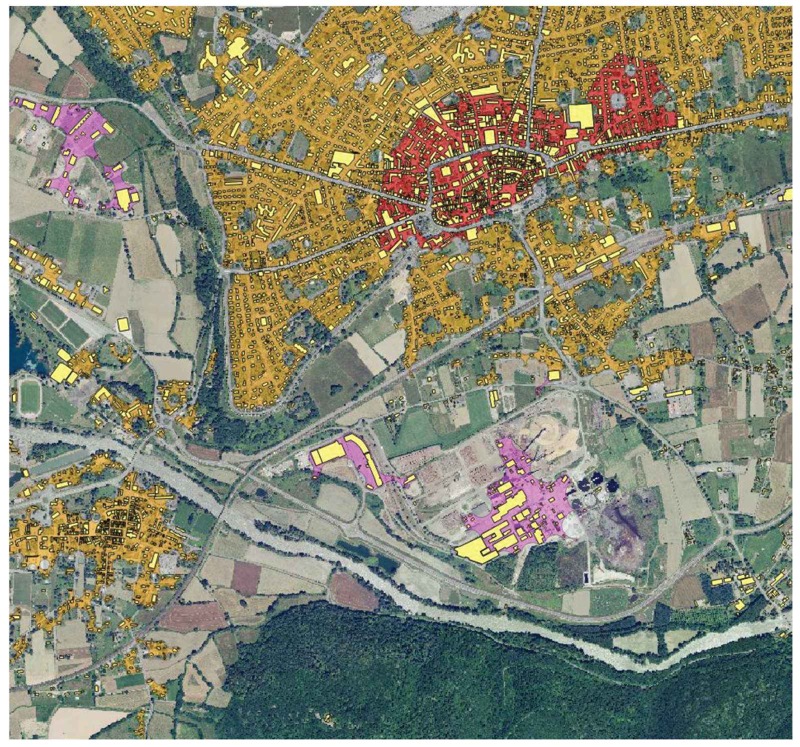
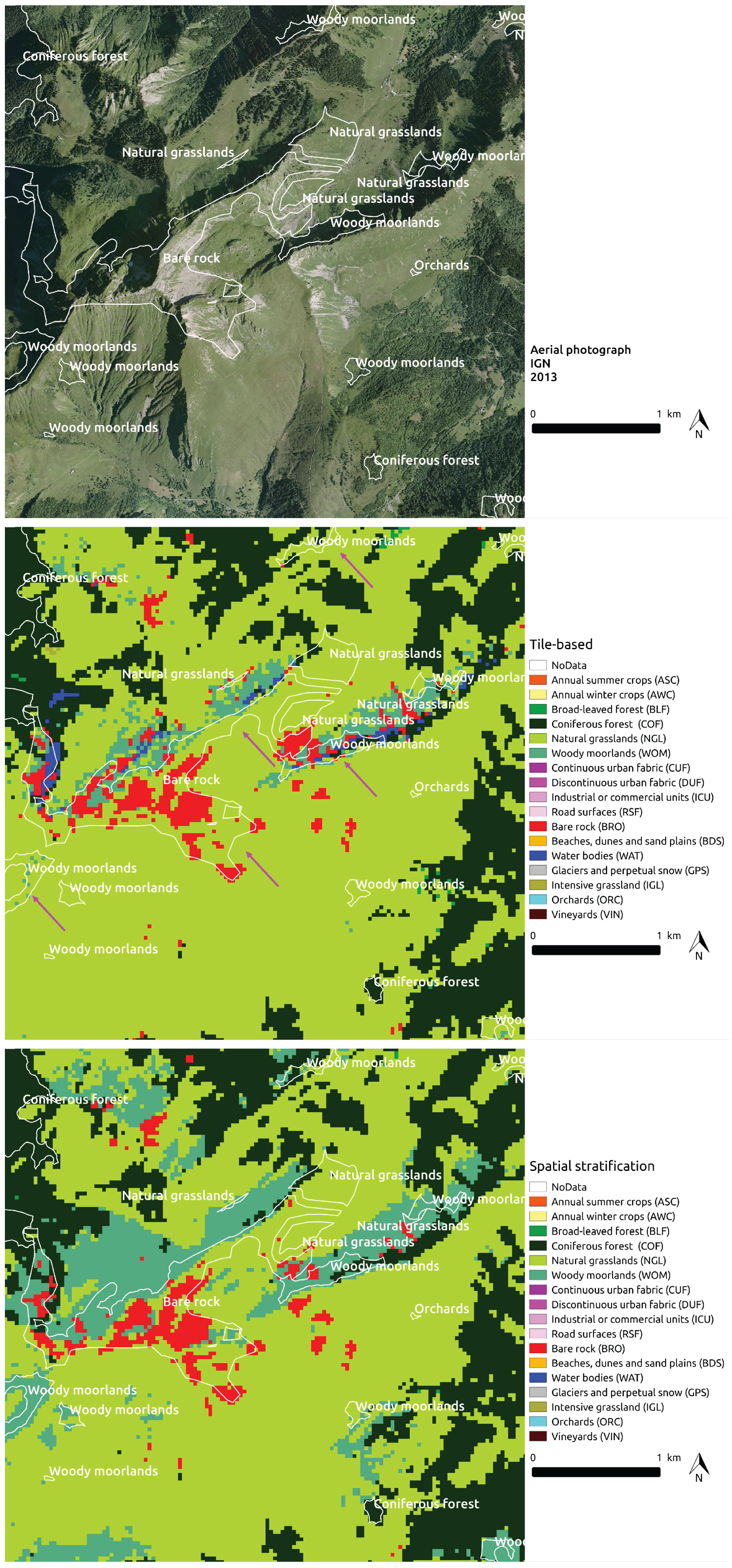
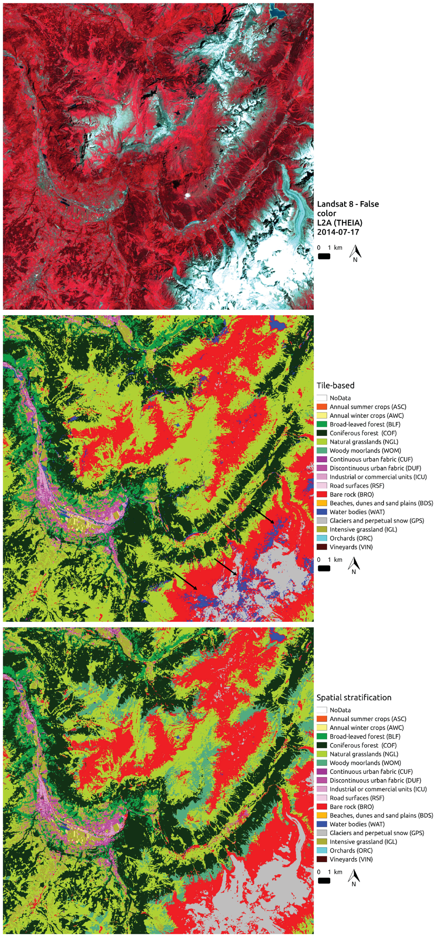
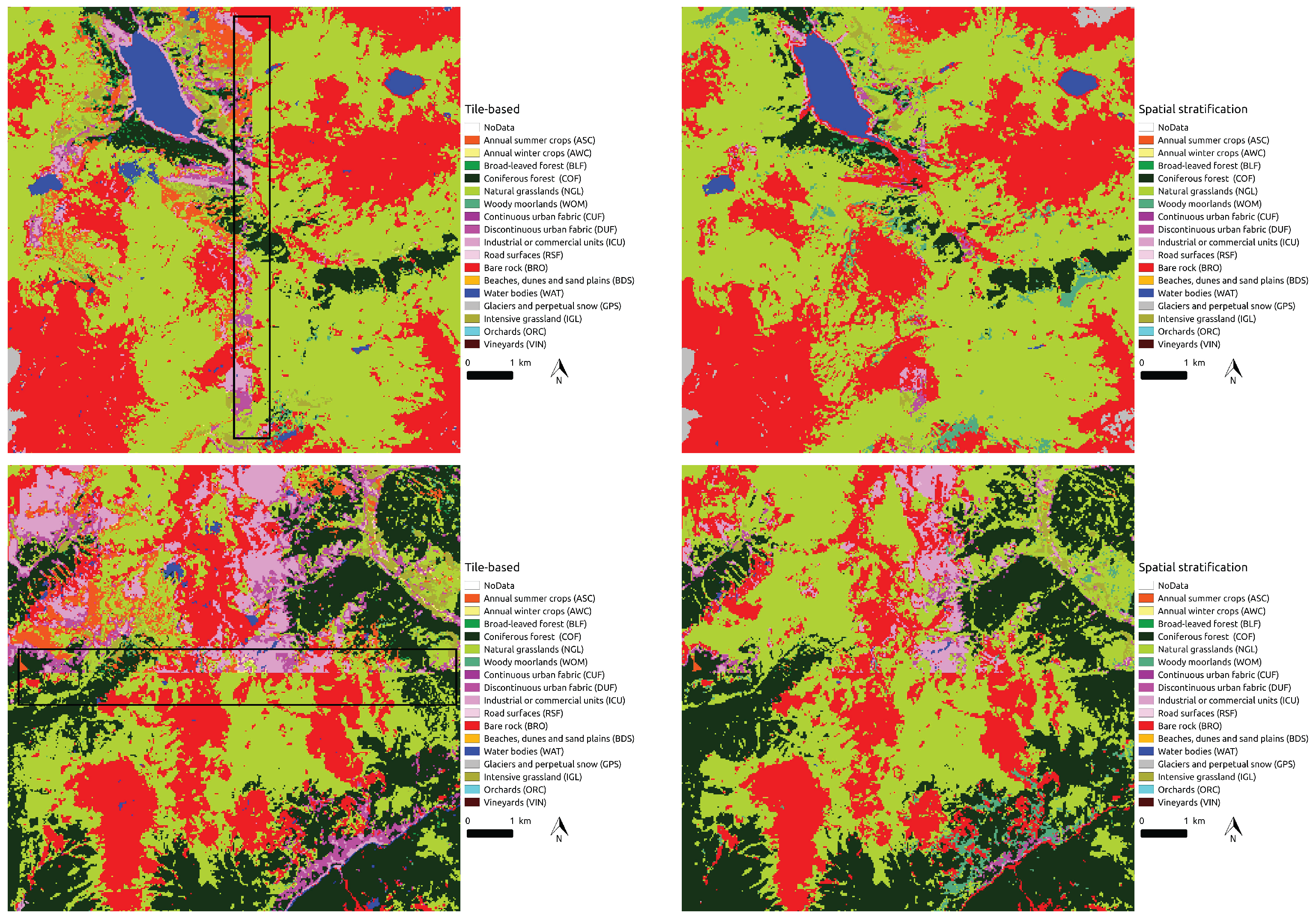
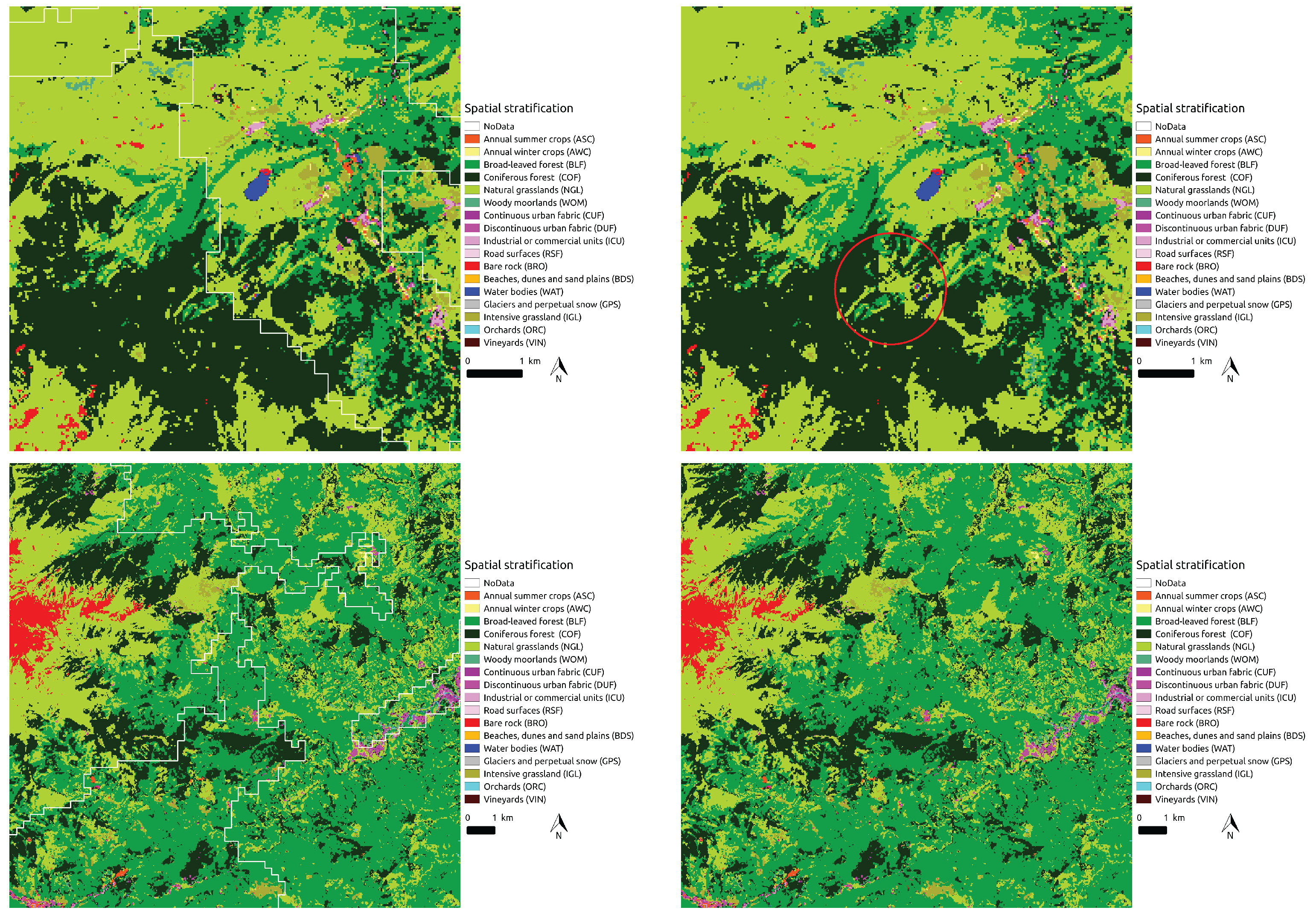
5.3. Visual Inspection

Quantitative metrics over a very large area are not able to reveal several kinds of errors present in the land cover maps. A visual inspection allows to identify different problems which are analysed in this section.

5.3.1. Difficult Landscapes

Fragmented areas or regions with irregular topography are much more difficult to map correctly than flat areas with large homogeneous landscapes.
Mountain areas are difficult to map because of the effects of the slopes on the signal measured by the satellite, but also because of the influence of slope, altitude and sun-facing condition on the distribution and characteristics of the land cover classes. Figure 19 illustrates this issue in an area in the Alps (Savoie region). It is worth noting that the aerial image does not help much to confidently distinguish natural grasslands and woody moorlands. The eco-climatic stratification is better able to capture the limits of the different classes, although the woody moorlands class remains difficult to detect. The mineral surfaces are correctly identified, and one can observe the correlation between south-facing slopes with natural grasslands and north-facing ones with woody moorlands.
Urban areas are difficult to map using 30 m Landsat-8 images because of the small size of the objects. Figure 20 illustrates an urban area near Toulouse, in the south of France. In this case, if one tries to distinguish the 4 urban classes, one can see that the eco-climatic stratification allows to better separate the discontinuous urban fabric and the industrial or commercial units, but these 2 classes remain confused. The road surfaces class is not detected and is classified as industrial or commercial units. This may be due to the coarse resolution of Landsat compared with that of Sentinel-2 time series at 10 m resolution.

5.3.2. Small, Local Classes

Minority classes are difficult to map because of their lack of representativity during the classifier training. Typical examples of these classes are glaciers and perpetual snow and beaches, dunes and sand. These classes are also concentrated in specific areas of the country. Figure 21 illustrates how the eco-climatic stratification reduces the confusion between water bodies and glaciers and perpetual snow. Figure 22 illustrates the same kind of behaviour but for the confusions between beaches, dunes and sand and urban areas.

5.3.3. Artefacts

As described in Section 4.3.1, the image data used for the map production does not offer an homogeneous cover of the country. Discontinuities are due to cloud cover and cloud shadows, satellite swath limits and absence of some acquisitions. The pre-processing step (geometric and radiometric corrections) can also discard some acquired images because of quality criteria: for instance, images with a very high cloud cover (higher than 90%) may not allow homologous point extraction for ortho-rectification or atmospherical optical thickness estimation needed for surface reflectance estimation. This can eliminate complete Landsat scenes (in the ortho-rectification step) or tiles (in the atmospheric correction step). All this impacts the quality of the temporal gapfilling and resampling, making adjacent pixels which should be nearly identical, be very different. The final consequence is that these pixels may be assigned to different classes when they should belong to the same one.
Another source of similar artefacts comes from the fact that several classification models are trained with different sets of samples. In the tile-based approach, all trained models are used for the classification step and the majority class is chosen. In the case of a tie, the class chosen by the model trained with samples belonging to the current image tile is chosen. In the case of the eco-climatic stratification, each region is classified independently. Both these approaches can introduce discontinuities, at the tile limits for the first one, and at the region limits for the second one.
These errors are rare and therefore do not have weight in the statistical quality metrics, but can be visually annoying or locally significant on the maps. Figure 23 illustrates some artefacts present on the limits of one tile to the East (upper row) and to the South (lower row) of a mountain area. One can observe that some artefacts disappear in the case of the eco-climatic mode (right column), but others remain because they are likely due to the pre-processing step as described above.
The spatial artefacts caused by the eco-climatic stratification can also be identified in some cases. Figure 24 illustrates 2 different areas of the map produced with stratification with the region limits superimposed in (left column). The upper example clearly shows some artefacts due to the stratification, but often, the limits of the eco-climatic regions coincide with land-cover changes, as it is the case in the south-east part of the image. The example of the bottom of the figure presents a very complex region for which the artefacts are very difficult to spot.

6. Conclusions

This paper has presented a methodology for the fully automatic production of land cover maps at country scale using high resolution optical image time series which is based on supervised classification and uses existing databases as reference data for training and validation. The originality of the approach resides in the use of all available image data (no scene selection in terms of appropriate dates or cloud cover), a simple pre-processing step leading to a homogeneous set of acquisition dates over the whole area (despite of using several satellite tracks and the presence of clouds and their shadows) and the use of a supervised classifier which is robust to errors in the reference data (databases which can be out of date, for instance). The use of a climatic stratification in the classification step has proven to yield significant improvements in terms of class recognition.
The processing is efficient, allowing a fast delivery of the maps after the acquisition of the image data, does not need expensive field surveys for model calibration and validation, nor human operators for decision making, and uses open and freely available imagery (Landsat-8 in our examples, and Sentinel-2 in the 2016 map to be produced at the beginning of 2017). The land cover maps are provided with a confidence map which gives information at the pixel level about the expected quality of the result.
However, the procedure still suffers from some drawbacks which need to be addressed. As indicated by the confidence maps, the quality of the classification strongly depends on the amount of cloud-free imagery in every given point. The authors have already investigated the contribution of Sentinel-1 SAR time series [48] and the processing chain has been updated to jointly use optical and SAR image time series.
Another critical issue is the availability of reference data for the so-called annual classes. Indeed, the Random Forest classifier has been shown to be robust to errors in the reference data (up to 15%), which allows to use out of date databases (for most classes, the rate of change is lower than 5% per year). However, classes such as annual crops, may change every year on every single point of the map: although the field remains an annual crop, it may change from wheat to corn, which results in a change from winter to summer crop. Therefore, a database older than one year is useless in our setting. Although the problem is solved at the French national level by using up to date data for these classes, or simple rules as the ones proposed in [49], one can argue that the proposed procedure lacks genericity and may therefore be difficult to apply to other regions of the world. In order to solve this issue, ongoing research by these authors shows promising results using relatively simple domain adaptation techniques which exploit time series from the previous years.
Despite the fact that the levels of accuracy obtained with the proposed procedure are higher than most comparable (in terms of areas covered and number of classes) state-of-the-art approaches, some classes suffer from poor recognition. Some of these classes could benefit from the use of very high spatial resolution (VHSR) imagery. The use of this kind of data (1 m resolution, single date acquisitions) is being investigated to lower the confusion between the urban classes. Other classes, such as natural grasslands or woody moorlands may also benefit from VHSR imagery, but will also need a more detailed investigation in terms of the exploitation of the temporal information. Indeed, the proposed approach simply stacks the image time series without explicitly extracting temporal features to lower the burden on the classification algorithm.
Finally, it is worth noting that achieving accuracies of about 90% may be enough for static land cover maps, but is close to useless in the frame of pixel-level land cover change analysis, since, as stated above, most of the classes have a rate of change closer to 5%. In this case, comparing land cover maps of successive years does not allow to accurately detect land cover evolutions. As a consequence, specific methods for accurate land cover change will have to be developed in the near future.

Acknowledgments

This work was supported by the CNES under the TOSCA programme. The authors would like to thank CESBIO colleagues (J-F. Dejoux, Ch. Pelletier and S. Valero) for their comments on earlier versions of this manuscript.

Author Contributions

Jordi Inglada is the main author of this manuscript, he designed and coordinated the research and the implementation of the processing chain, and participated in the analysis and interpretation of the results. Arthur Vincent is the main developer of the processing chain and participated in the analysis and interpretation of the results. Marcela Arias participated in the early stages of the development of the processing chain and participated in the analysis and interpretation of the results. Benjamin Tardy participated in the early stages of the development of the processing chain. David Morin produced most of the analysis of the results presented in this manuscript. Isabel Rodes, while working on her PhD, participated in some of the discussions which led to the design of the architecture of the processing chain.

Conflicts of Interest

The authors declare no conflict of interest.

References

  1. Bojinski, S.; Verstraete, M.; Peterson, T.C.; Richter, C.; Simmons, A.; Zemp, M. The concept of essential climate variables in support of climate research, applications, and policy. Bull. Am. Meteorol. Soc. 2014, 95, 1431–1443. [Google Scholar] [CrossRef]
  2. Heymann, Y. CORINE Land Cover: Technical Guide; Office for Official Publications of the European Communities: Luxembourg, 1994. [Google Scholar]
  3. Drusch, M.; Bello, U.D.; Carlier, S.; Colin, O.; Fernandez, V.; Gascon, F.; Hoersch, B.; Isola, C.; Laberinti, P.; Martimort, P.; et al. Sentinel-2: ESA’s optical high-resolution mission for GMES operational services. Remote Sens. Environ. 2012, 120, 25–36. [Google Scholar] [CrossRef]
  4. Whitcraft, A.; Becker-Reshef, I.; Justice, C. A framework for defining spatially explicit earth observation requirements for a global agricultural monitoring initiative (GEOGLAM). Remote Sens. 2015, 7, 1461–1481. [Google Scholar] [CrossRef]
  5. Whitcraft, A.; Becker-Reshef, I.; Killough, B.; Justice, C. Meeting earth observation requirements for global agricultural monitoring: An evaluation of the revisit capabilities of current and planned moderate resolution optical earth observing missions. Remote Sens. 2015, 7, 1482–1503. [Google Scholar] [CrossRef]
  6. Irons, J.R.; Dwyer, J.L.; Barsi, J.A. The next Landsat satellite: The Landsat data continuity mission. Remote Sens. Environ. 2012, 122, 11–21. [Google Scholar] [CrossRef]
  7. Inglada, J.; Arias, M.; Tardy, B.; Hagolle, O.; Valero, S.; Morin, D.; Dedieu, G.; Sepulcre, G.; Bontemps, S.; Defourny, P.; et al. Assessment of an operational system for crop type map production using high temporal and spatial resolution satellite optical imagery. Remote Sens. 2015, 7, 12356–12379. [Google Scholar] [CrossRef]
  8. Arino, O.; Gross, D.; Ranera, F.; Leroy, M.; Bicheron, P.; Brockman, C.; Defourny, P.; Vancutsem, C.; Achard, F.; Durieux, L.; et al. GlobCover: ESA service for global land cover from MERIS. In Proceedings of the 2007 IEEE International Geoscience and Remote Sensing Symposium, Barcelona, Spain, 23–28 July 2007.
  9. Foody, G.M.; Mathur, A.; Sanchez-Hernandez, C.; Boyd, D.S. Training set size requirements for the classification of a specific class. Remote Sens. Environ. 2006, 104, 1–14. [Google Scholar] [CrossRef]
  10. Stehman, S.V. Sampling designs for accuracy assessment of land cover. Int. J. Remote Sens. 2009, 30, 5243–5272. [Google Scholar] [CrossRef]
  11. Bruzzone, L.; Chi, M.; Marconcini, M. A novel transductive SVM for semisupervised classification of remote-sensing images. IEEE Trans. Geosci. Remote Sens. 2006, 44, 3363–3373. [Google Scholar] [CrossRef]
  12. Bruzzone, L.; Marconcini, M. Domain adaptation problems: A DASVM classification technique and a circular validation strategy. IEEE Trans. Pattern Anal. Mach. Intell. 2010, 32, 770–787. [Google Scholar] [CrossRef] [PubMed]
  13. Matasci, G.; Volpi, M.; Kanevski, M.; Bruzzone, L.; Tuia, D. Semisupervised transfer component analysis for domain adaptation in remote sensing image classification. IEEE Trans. Geosci. Remote Sens. 2015, 53, 3550–3564. [Google Scholar] [CrossRef]
  14. Petitjean, F.; Inglada, J.; Gancarski, P. Satellite image time series analysis under time warping. IEEE Trans. Geosci. Remote Sens. 2012, 50, 3081–3095. [Google Scholar] [CrossRef]
  15. Defries, R.S.; Townshend, J.R.G. Global land cover characterization from satellite data: From research to operational implementation. GCTE/LUCC research review. Glob. Ecol. Biogeogr. 1999, 8, 367–379. [Google Scholar] [CrossRef]
  16. Hansen, M.C.; Loveland, T.R. A review of large area monitoring of land cover change using Landsat data. Remote Sens. Environ. 2012, 122, 66–74. [Google Scholar] [CrossRef]
  17. Chen, J.; Chen, J.; Liao, A.; Cao, X.; Chen, L.; Chen, X.; He, C.; Han, G.; Peng, S.; Lu, M.; et al. Global land cover mapping at 30m resolution: A POK-based operational approach. ISPRS J. Photogramm. Remote Sens. 2015, 103, 7–27. [Google Scholar] [CrossRef]
  18. Grekousis, G.; Mountrakis, G.; Kavouras, M. An overview of 21 global and 43 regional land-cover mapping products. Int. J. Remote Sens. 2015, 36, 1–27. [Google Scholar] [CrossRef]
  19. Gong, P.; Wang, J.; Yu, L.; Zhao, Y.; Zhao, Y.; Liang, L.; Niu, Z.; Huang, X.; Fu, H.; Liu, S.; et al. Finer resolution observation and monitoring of global land cover: First mapping results with Landsat TM and ETM+ Data. Int. J. Remote Sens. 2013, 34, 2607–2654. [Google Scholar] [CrossRef]
  20. Yu, L.; Wang, J.; Gong, P. Improving 30 m global land-cover map from-GLC with time series MODIS and auxiliary data sets: A segmentation-based approach. Int. J. Remote Sens. 2013, 34, 5851–5867. [Google Scholar] [CrossRef]
  21. Yu, L.; Wang, J.; Li, X.; Li, C.; Zhao, Y.; Gong, P. A multi-resolution global land cover dataset through multisource data aggregation. Sci. China Earth Sci. 2014, 57, 2317–2329. [Google Scholar] [CrossRef]
  22. Giri, C.; Long, J. Land cover characterization and mapping of South America for the year 2010 using Landsat 30 m satellite data. Remote Sens. 2014, 6, 9494–9510. [Google Scholar] [CrossRef]
  23. Homer, C.; Dewitz, J.; Fry, J.; Coan, M.; Hossain, N.; Larson, C.; Herold, N.; McKerrow, A.; VanDriel, J.N.; Wickham, J.; et al. Completion of the 2001 national land cover database for the counterminous United States. Photogramm. Eng. Remote Sens. 2007, 73, 337. [Google Scholar]
  24. Jin, S.; Yang, L.; Danielson, P.; Homer, C.; Fry, J.; Xian, G. A comprehensive change detection method for updating the national land cover database to circa 2011. Remote Sens. Environ. 2013, 132, 159–175. [Google Scholar] [CrossRef]
  25. Deng, X.; Liu, J. Mapping land cover and land use changes in China. In Remote Sensing of Land Use and Land Cover: Principles and Applications; CRC Press: Boca Raton, FL, USA, 2012; pp. 339–349. [Google Scholar]
  26. Zhang, Z.; Wang, X.; Zhao, X.; Liu, B.; Yi, L.; Zuo, L.; Wen, Q.; Liu, F.; Xu, J.; Hu, S. A 2010 update of national land use/cover database of China at 1:100000 scale using medium spatial resolution satellite images. Remote Sens. Environ. 2014, 149, 142–154. [Google Scholar] [CrossRef]
  27. Congalton, R.; Gu, J.; Yadav, K.; Thenkabail, P.; Ozdogan, M. Global land cover mapping: A review and uncertainty analysis. Remote Sens. 2014, 6, 12070–12093. [Google Scholar] [CrossRef]
  28. Peel, M.C.; Finlayson, B.L.; McMahon, T.A. Updated world map of the Köppen-Geiger climate classification. Hydrol. Earth Syst. Sci. 2007, 11, 1633–1644. [Google Scholar] [CrossRef]
  29. Bossard, M.; Feranec, J.; Otahel, J. CORINE Land Cover Technical Guide. Addendum 2000; European Environment Agency: Copenhagen, Denmark, 2000. [Google Scholar]
  30. Maugeais, E.; Lecordix, F.; Halbecq, X.; Braun, A. Dérivation cartographique multi échelles de la BDTopo de l’IGN France: Mise en œuvre du processus de production de la Nouvelle Carte de Base. In Proceedings of the 25th International Cartographic Conference, Paris, France, 3–8 July 2011; pp. 3–8.
  31. Cantelaube, P.; Carles, M. Le registre parcellaire graphique: Des données géographiques pour décrire la couverture du sol agricole. In Le Cahier des Techniques de l’INRA; INRA: Paris, France, 2014; pp. 58–64. [Google Scholar]
  32. Pfeffer, W.T.; Arendt, A.A.; Bliss, A.; Bolch, T.; Cogley, J.G.; Gardner, A.S.; Hagen, J.O.; Hock, R.; Kaser, G.; Kienholz, C.; et al. The randolph glacier inventory: A globally complete inventory of glaciers. J. Glaciol. 2014, 60, 537–552. [Google Scholar] [CrossRef] [Green Version]
  33. Joly, D.; Brossard, T.; Cardot, H.; Cavailhes, J.; Hilal, M.; Wavresky, P. Les types de climats en France, une construction spatiale. Cybergeo 2010. [Google Scholar] [CrossRef]
  34. Hagolle, O.; Sylvander, S.; Huc, M.; Claverie, M.; Clesse, D.; Dechoz, C.; Lonjou, V.; Poulain, V. SPOT4 (Take5): Simulation of sentinel-2 time series on 45 large sites. Remote Sens. 2015, 7, 12242–12264. [Google Scholar] [CrossRef]
  35. Inglada, J.; Vincent, A.; Arias, M.; Tardy, B. iota2-a25386. 2016. Available online: http://tully.ups-tlse.fr/jordi/iota2 (assessed on 18 January 2017).
  36. Inglada, J.; Christophe, E. The Orfeo Toolbox remote sensing image processing software. In Proceedings of the 2009 IEEE International Geoscience and Remote Sensing Symposium, Cape Town, South Africa, 12–17 July 2009; Volume 4, pp. IV-733–IV-736.
  37. Michel, J.; Grizonnet, M. State of the Orfeo Toolbox. In Proceedings of the 2015 IEEE International Geoscience and Remote Sensing Symposium (IGARSS), Milan, Italy, 26–31 July 2015; pp. 1336–1339.
  38. OTB Development Team. Orfeo Toolbox 5.4. Available online: https://git.orfeo-toolbox.org/otb.git/tag/faf53491eabbd6f30672c0132afb61737e9f47f6 (assessed on 18 January 2017).
  39. Inglada, J. OTB Gapfilling, a Temporal Gapfilling for Image Time Series Library. 2016. Available online: http://tully.ups-tlse.fr/jordi/temporalgapfilling (assessed on 18 January 2017).
  40. Arias, M.; Morin, D. Vector-Tools-7ab2125a. 2016. Available online: http://tully.ups-tlse.fr/jordi/vector_tools (assessed on 18 January 2017).
  41. Tucker, C.J. Red and photographic infrared linear combinations for monitoring vegetation. Remote Sens. Environ. 1979, 8, 127–150. [Google Scholar] [CrossRef]
  42. Gao, B.C. NDWI. A normalized difference water index for remote sensing of vegetation liquid water from space. Remote Sens. Environ. 1996, 58, 257–266. [Google Scholar] [CrossRef]
  43. Breiman, L. Random forests. Mach. Learn. 2001, 45, 5–32. [Google Scholar] [CrossRef]
  44. Folleco, A.; Khoshgoftaar, T.M.; Hulse, J.V.; Bullard, L. Software quality modeling: The impact of class noise on the random forest classifier. In Proceedings of the 2008 IEEE Congress on Evolutionary Computation (IEEE World Congress on Computational Intelligence), Hong Kong, China, 1–6 June 2008.
  45. Frenay, B.; Verleysen, M. Classification in the presence of label noise: A survey. IEEE Trans. Neural Netw. Learn. Syst. 2014, 25, 845–869. [Google Scholar] [CrossRef] [PubMed]
  46. Pelletier, C.; Valero, S.; Inglada, J.; Champion, N.; Dedieu, G. Assessing the robustness of random forests to map land cover with high resolution satellite image time series over large areas. Remote Sens. Environ. 2016, 187, 156–168. [Google Scholar] [CrossRef]
  47. Mellor, A.; Boukir, S.; Haywood, A.; Jones, S. Exploring issues of training data imbalance and mislabelling on random forest performance for large area land cover classification using the ensemble margin. ISPRS J. Photogramm. Remote Sens. 2015, 105, 155–168. [Google Scholar] [CrossRef]
  48. Inglada, J.; Vincent, A.; Arias, M.; Marais-Sicre, C. Improved early crop type identification by joint use of high temporal resolution SAR and optical image time series. Remote Sens. 2016, 8, 362. [Google Scholar] [CrossRef]
  49. Sicre, C.M.; Inglada, J.; Fieuzal, R.; Baup, F.; Valero, S.; Cros, J.; Huc, M.; Demarez, V. Early detection of summer crops using high spatial resolution optical image time series. Remote Sens. 2016, 8, 591. [Google Scholar] [CrossRef]
Figure 1. Study area, metropolitan France not including Corsica. Adapted from Wikimedia Commons (original map by Delphi234) CC BY-SA 4.0. https://commons.wikimedia.org/w/index.php?curid=38255428.
Remotesensing 09 00095 g001
Figure 2. Eco-climatic area map for the study area from [33].
Remotesensing 09 00095 g002
Figure 3. Block diagram of the land cover map production procedure.
Remotesensing 09 00095 g003
Figure 4. Reference data cleansing.
Remotesensing 09 00095 g004
Figure 5. Before refinement of urban classes: individual buildings from BD-Topo in yellow, Continuous Urban Fabric (CUF) in red, Discontinuous Urban Fabric (DUF) in orange and Industrial and Commercial Units (ICU) in pink.
Remotesensing 09 00095 g005
Figure 6. After refinement of urban classes: individual buildings from BD-Topo in yellow, Continuous Urban Fabric (CUF) in red, Discontinuous Urban Fabric (DUF) in orange and Industrial and Commercial Units (ICU) in pink.
Remotesensing 09 00095 g006
Figure 7. Path-row grid for Landsat acquisitions. Every path (North-South track) is acquired on the same date every 16 days. Adjacent paths are acquired 8 days apart.
Remotesensing 09 00095 g007
Figure 8. Map of the number of times that every pixel sees the ground taking into account satellite revisit and cloud cover.
Remotesensing 09 00095 g008
Figure 9. Histogram of the number of times that every pixel sees the ground taking into account satellite revisit and cloud cover.
Remotesensing 09 00095 g009
Figure 10. Image tiling for storage and processing. The green squares are the 78 tiles of size 110 km × 110 km needed to cover the study site. Landsat acquisitions are represented in yellow.
Remotesensing 09 00095 g010
Figure 11. Tiled-based approach for classifier training. Each colour identifies the subset of tiles for which a common classifier is trained.
Remotesensing 09 00095 g011
Figure 12. Land cover map for France for the year 2014 using the proposed methodology.
Remotesensing 09 00095 g012
Figure 13. Performance metrics for the produced maps.
Remotesensing 09 00095 g013
Figure 14. FScore per class.
Remotesensing 09 00095 g014
Figure 15. Recall per class.
Remotesensing 09 00095 g015
Figure 16. Precision per class.
Remotesensing 09 00095 g016
Figure 17. Confidence map: percentage of trees of the RF classifier which voted for the majority class.
Remotesensing 09 00095 g017
Figure 18. Confidence statistics.
Remotesensing 09 00095 g018
Figure 19. Analysis of errors on a mountain area. Errors are marked with magenta arrows.
Remotesensing 09 00095 g019
Figure 20. Analysis of errors on an urban area. Errors are marked with black arrows.
Remotesensing 09 00095 g020
Figure 21. Analysis of errors over snow and ice. Examples of water over detection are indicated with black arrows.
Remotesensing 09 00095 g021
Figure 22. Analysis of errors over sand areas. Examples of sand misclassifications are indicated with black arrows.
Remotesensing 09 00095 g022
Figure 23. Analysis of artefacts due to tiling. Tile transitions with important artefacts are indicated with black rectangles.
Remotesensing 09 00095 g023
Figure 24. Analysis of artefacts due to eco-climatic stratification. The red circle shows errors due to the boundaries of climatic areas for the upper row example. The lower row example does not show artefacts.
Remotesensing 09 00095 g024
Table 1. Landsat-8 scenes.
PathRow#DatesDate List
194291701-24 02-09 02-25 03-13 03-29 04-14
05-16 06-01 07-03 07-19 08-04 08-20
09-05 10-23 11-08 12-10 12-26
194301501-24 02-09 02-25 03-13 04-14 05-16
06-01 06-17 07-03 08-20 09-05 10-23
11-08 12-10 12-26
19526901-15 03-04 04-21 05-23 06-08 06-24
08-11 09-28 10-14
19527901-15 01-31 03-20 05-23 06-08 09-12
09-28 10-14 10-30
19528901-31 03-20 05-23 06-08 08-27 09-12
09-28 10-14 10-30
195291601-15 01-31 03-04 03-20 04-05 05-07
05-23 06-08 06-24 07-10 07-26 08-11
08-27 09-12 09-28 10-30
195301701-15 01-31 02-16 03-04 03-20 04-05
05-07 05-23 06-08 06-24 07-10 07-26
08-11 08-27 09-12 09-28 10-30
196261201-06 02-23 03-11 03-27 04-12 05-14
06-15 07-01 07-17 09-03 09-19 11-22
196271701-22 02-23 03-11 03-27 04-12 05-14
05-30 06-15 07-01 07-17 08-18 09-03
09-19 10-21 11-06 11-22 12-24
196281801-06 01-22 02-23 03-11 03-27 04-12
05-14 05-30 06-15 07-01 07-17 08-18
09-03 10-05 10-21 11-06 11-22 12-24
196291901-06 01-22 02-23 03-11 03-27 04-12
04-28 05-14 05-30 07-01 07-17 08-02
08-18 09-03 10-21 11-06 11-22 12-08
12-24
196302001-06 01-22 02-23 03-11 03-27 04-12
04-28 05-14 05-30 06-15 07-01 07-17
08-02 08-18 09-03 09-19 10-05 10-21
11-06 12-24
19725701-29 04-03 05-05 06-06 06-22 07-24
09-26
197261303-02 03-18 04-03 04-19 05-05 06-06
06-22 07-24 08-09 09-10 09-26 11-13
12-15
197271603-02 03-18 04-19 05-05 06-06 06-22
07-08 07-24 08-09 08-25 09-10 09-26
10-28 11-13 12-15 12-31
197281403-02 03-18 04-19 05-05 06-06 06-22
07-24 08-09 08-25 09-10 09-26 10-28
11-13 12-15
197291703-02 03-18 04-19 05-05 05-21 06-22
07-08 07-24 08-09 08-25 09-10 09-26
10-12 10-28 11-13 12-15 12-31
197301901-29 02-14 03-02 03-18 04-19 05-05
05-21 06-06 06-22 07-24 08-09 08-25
09-10 09-26 10-12 10-28 11-13 12-15
12-31
197311501-29 02-14 03-02 03-18 04-19 05-05
06-06 06-22 07-08 08-09 08-25 09-26
10-12 11-13 12-31
198251402-05 02-21 03-09 03-25 04-10 06-13
07-31 08-16 09-01 09-17 10-03 10-19
11-20 12-06
198261102-21 03-09 03-25 04-10 06-13 07-31
08-16 09-01 09-17 10-03 10-19
198271302-21 03-09 04-10 05-28 06-13 07-31
08-16 09-01 09-17 10-03 10-19 11-20
12-22
198281303-09 04-10 05-28 06-13 06-29 07-31
08-16 09-01 09-17 10-03 10-19 11-20
12-22
198291203-09 04-10 05-28 06-13 07-31 08-16
09-01 09-17 10-03 10-19 11-20 12-22
198301801-20 03-09 03-25 04-10 04-26 05-12
05-28 06-13 06-29 07-31 08-16 09-01
09-17 10-03 10-19 11-20 12-06 12-22
198311701-04 01-20 03-09 03-25 04-10 05-12
05-28 06-13 06-29 07-31 08-16 09-01
09-17 10-03 10-19 11-20 12-06
199241101-11 02-12 03-16 05-03 05-19 06-20
08-07 08-23 09-08 11-11 12-29
199251102-12 03-16 04-01 04-17 05-19 08-07
08-23 09-08 10-10 10-26 11-11
199261601-11 01-27 02-12 02-28 03-16 04-01
04-17 05-03 05-19 08-23 09-08 09-24
10-10 10-26 11-11 12-29
199271501-27 02-12 02-28 03-16 04-01 04-17
05-03 05-19 06-20 09-08 09-24 10-26
11-11 11-27 12-29
199281601-27 02-12 02-28 03-16 04-01 04-17
05-19 06-04 06-20 07-22 09-08 09-24
10-26 11-11 11-27 12-29
199291302-12 03-16 04-01 04-17 05-19 06-04
06-20 07-22 09-08 10-26 11-11 11-27
12-29
199302001-11 01-27 02-12 02-28 03-16 04-01
04-17 05-03 05-19 06-04 06-20 07-22
08-07 08-23 09-08 09-24 10-26 11-11
11-27 12-29
19931106-04
20024701-02 02-03 03-23 04-08 09-15 11-02
12-20
200251301-02 02-03 03-07 03-23 04-08 06-11
08-14 09-15 10-01 10-17 11-02 11-18
12-20
20026901-02 01-18 02-03 03-07 04-08 06-11
06-27 09-15 10-01
200271001-02 01-18 02-03 03-07 03-23 06-11
06-27 08-30 09-15 10-01
200281701-02 01-18 02-03 03-07 03-23 04-08
06-11 06-27 07-29 08-14 08-30 09-15
10-01 10-17 11-02 11-18 12-20
200291401-02 02-19 03-07 03-23 04-08 06-11
06-27 07-29 08-14 08-30 09-15 10-01
10-17 11-18
200301602-19 03-07 03-23 04-08 05-10 05-26
06-11 06-27 07-13 07-29 08-14 09-15
10-01 10-17 11-18 12-04
201251301-09 02-26 04-15 05-17 06-02 06-18
07-04 08-21 09-22 10-08 11-09 12-11
12-27
201261601-25 02-26 03-14 03-30 04-15 05-17
06-18 07-04 08-05 08-21 09-06 09-22
10-08 11-09 12-11 12-27
201271701-25 02-26 03-14 03-30 04-15 05-17
06-02 06-18 07-04 08-05 08-21 09-06
09-22 10-08 10-24 11-09 12-27
201281601-25 02-26 03-14 03-30 04-15 05-17
06-02 06-18 07-04 08-05 08-21 09-06
09-22 10-08 10-24 11-09
20129803-14 04-15 06-18 07-20 08-05 08-21
09-22 10-24
201301101-25 02-26 03-14 04-15 05-01 05-17
06-02 06-18 08-21 09-06 10-08
202251001-16 03-05 03-21 05-24 06-09 06-25
07-11 08-12 08-28 10-31
202261301-16 02-01 03-05 03-21 05-24 06-09
06-25 07-11 08-12 08-28 09-29 10-31
11-16
202271501-16 02-01 03-05 03-21 04-22 05-24
06-09 06-25 07-27 08-12 08-28 09-13
09-29 10-31 11-16
203261901-07 01-23 02-08 02-24 03-12 04-13
05-15 05-31 06-16 07-02 07-18 08-03
08-19 09-04 09-20 10-06 10-22 11-07
12-25
203271701-07 02-08 02-24 03-12 05-15 05-31
06-16 07-02 07-18 08-03 08-19 09-04
10-06 10-22 11-07 12-09 12-25
204261104-04 05-06 06-07 06-23 07-09 07-25
08-10 08-26 09-11 09-27 10-13
20427801-14 04-04 06-07 06-23 08-10 09-11
09-27 10-13
Table 2. Confusion matrix for the tile-based approach. Columns represent produced labels and rows represent the reference labels. Values are given in percentage of reference pixels (normalised per row). Diagonal values represnent the recall for each class.
ASCAWCBLFCOFNGLWOMCUFDUFICURSFBROBDSWATGPSIGLORCVIN
ASC91.192.660.370.380.390.080.012.440.370.000.000.010.150.001.650.000.29
AWC0.6797.140.070.150.130.030.000.830.140.000.000.010.070.000.720.000.05
BLF0.190.1886.986.741.940.520.000.830.020.000.000.000.180.002.400.000.03
COF0.810.314.6085.823.031.760.002.650.080.000.060.000.160.000.480.000.23
NGL0.970.753.886.9364.183.020.007.700.330.002.420.010.150.019.120.000.55
WOM1.270.768.4713.7133.7212.360.0013.911.110.002.370.032.250.009.850.000.20
CUF0.170.060.250.610.130.0814.0255.1128.820.000.030.010.540.000.160.000.03
DUF0.500.720.951.360.890.090.4184.037.550.000.090.010.190.003.110.000.12
ICU0.370.650.850.790.450.100.3938.1556.320.000.030.020.360.001.460.000.05
RSF0.430.950.540.580.800.060.0922.6271.390.000.550.070.470.001.390.000.05
BRO0.040.010.060.558.620.430.010.731.830.0084.530.022.460.690.010.000.00
BDS2.241.382.651.252.260.710.0116.0033.360.011.6318.3517.630.002.150.000.37
WAT0.090.080.160.150.100.260.000.190.230.000.020.0398.480.000.180.000.00
GPS0.000.000.000.001.530.000.000.000.000.0045.450.075.8647.090.000.000.00
IGL0.291.171.980.957.960.320.000.760.020.000.210.000.200.0086.100.000.03
ORC6.055.0118.332.186.000.980.0022.120.300.000.000.010.120.0033.452.732.70
VIN25.811.380.251.253.400.260.0018.210.230.000.000.070.080.005.490.0143.55
Table 3. Confusion matrix for the eco-climatic stratification approach. Columns represent produced labels and rows represent the reference labels. Values are given in percentage of reference pixels (normalised per row). Diagonal values represnent the recall for each class.
ASCAWCBLFCOFNGLWOMCUFDUFICURSFBROBDSWATGPSIGLORCVIN
ASC94.191.960.260.490.180.110.021.000.160.000.000.020.050.001.150.010.41
AWC0.6698.160.060.080.110.040.000.280.050.000.000.010.020.000.490.010.06
BLF0.150.1689.655.062.021.170.000.330.020.000.000.000.110.001.250.010.05
COF0.240.083.2092.541.791.080.000.510.060.000.070.010.020.000.340.000.06
NGL0.240.502.795.6364.578.340.001.400.180.002.680.040.130.0113.140.020.30
WOM0.540.455.689.4529.4741.030.001.840.290.002.580.142.910.005.340.030.26
CUF0.210.060.250.530.250.3224.8046.4726.230.010.110.110.270.000.130.010.25
DUF0.630.760.871.441.270.850.8482.077.760.000.180.050.110.002.760.040.40
ICU0.480.750.790.910.540.570.7334.3958.730.030.160.160.290.001.280.040.16
RSF0.510.930.500.670.930.820.3319.3171.281.340.880.450.560.001.330.030.13
BRO0.010.000.060.766.881.570.000.200.460.0086.220.060.223.390.180.000.00
BDS1.230.802.191.503.885.890.039.108.250.021.0443.0521.380.001.140.130.39
WAT0.050.050.110.060.080.480.000.050.060.000.040.1298.740.000.150.000.01
GPS0.000.000.000.000.420.000.000.000.000.0014.470.010.0585.050.000.000.00
IGL0.230.661.590.834.580.940.000.490.010.000.220.010.190.0090.140.020.09
ORC3.832.859.402.047.656.060.018.720.250.000.000.080.170.0021.7429.607.58
VIN5.731.080.241.501.990.880.023.940.090.000.000.040.070.002.190.1582.08

