Global Surface Mass Variations from Continuous GPS Observations and Satellite Altimetry Data


1
National Time Service Center, Chinese Academy of Sciences, Xi’an 710600, China
2
Shanghai Astronomical Observatory, Chinese Academy of Sciences, Shanghai 200030, China
*
Authors to whom correspondence should be addressed.
Remote Sens. 2017, 9(10), 1000; https://doi.org/10.3390/rs9101000
Submission received: 7 August 2017
/
Revised: 8 September 2017
/
Accepted: 22 September 2017
/
Published: 27 September 2017
(This article belongs to the Special Issue Multi-Constellation Global Navigation Satellite Systems: Methods and Applications)
Abstract
:The Gravity Recovery and Climate Experiment (GRACE) mission is able to observe the global large-scale mass and water cycle for the first time with unprecedented spatial and temporal resolution. However, no other time-varying gravity fields validate GRACE. Furthermore, the C20 of GRACE is poor, and no GRACE data are available before 2002 and there will likely be a gap between the GRACE and GRACE-FOLLOW-ON mission. To compensate for GRACE’s shortcomings, in this paper, we provide an alternative way to invert Earth’s time-varying gravity field, using a priori degree variance as a constraint on amplitudes of Stoke’s coefficients up to degree and order 60, by combining continuous GPS coordinate time series and satellite altimetry (SA) mean sea level anomaly data from January 2003 to December 2012. Analysis results show that our estimated zonal low-degree gravity coefficients agree well with those of GRACE, and large-scale mass distributions are also investigated and assessed. It was clear that our method effectively detected global large-scale mass changes, which is consistent with GRACE observations and the GLDAS model, revealing the minimums of annual water cycle in the Amazon in September and October. The global mean mass uncertainty of our solution is about two times larger than that of GRACE after applying a Gaussian spatial filter with a half wavelength at 500 km. The sensitivity analysis further shows that ground GPS observations dominate the lower-degree coefficients but fail to contribute to the higher-degree coefficients, while SA plays a complementary role at higher-degree coefficients. Consequently, a comparison in both the spherical harmonic and geographic domain confirms our global inversion for the time-varying gravity field from GPS and Satellite Altimetry.
1. Introduction
The Earth is a dynamic system. The motion of the Earth’s interior and surface mass, including the atmosphere, oceans, hydrology and glacier melting, causes the redistribution of Earth mass, deformation of the solid Earth and variations of the gravity field, which have different time and spatial scales. Precise determination of time variable global gravity is useful to model these dynamic processes [1,2,3,4,5,6,7].
For the last two decades, modern geodetic techniques have been the main tools to invert the gravity field. So far, Satellite Laser Ranging (SLR) is considered as an effective means to measure not only the seasonal variations but also secular trend of geocenter motion and low degree coefficients [8,9,10,11]. However, limited by the geographic location of SLR tracking stations and altitudes of SLR satellites, the SLR technique could supply some gravity information at long wavelength and could measure mass distribution of the Earth only in low degree and order terms [12]. Low degree gravity variations can also be estimated from GPS tracking of low earth satellites (LEOs) such as GRACE, GOCE, CHAMP and COSMIC [13,14,15].
However, neither the SLR nor GPS-LEO technique performs better than GRACE. GRACE, launched in 2002, consists of two identical satellites operating in the same orbit. By measuring the small changes between two satellites of GRACE, a time-varying gravity field has been determined in the spherical harmonic domain with a complete spectrum up to degree and order 60 for the first time, thus allowing to observe global large-scale mass redistribution [1,6,7,16]. However, GRACE data is not continuous and there is a lack of data in several months; presently, the life of GRACE has been prolonged and the new GRACE–FOLLOW-ON mission is to be launched in 2017, so there may be large data gap.
Since geocenter motion, due to the degree-1 load deformation, is closely related to the terrestrial reference frame origin, estimation of the geocenter could be helpful to constrain global mass redistribution and sea level signature. However, current geocenter timeseries disagree with environmental models. Furthermore, GRACE cannot observe geocenter motion directly. Another strategy to detect temporal variations in the degree-1 gravity field, known as surface loading inversion, was first presented by [17], in which geocenter motion was estimated and analyzed using 66 worldwide distributed GPS stations with higher-degree harmonics being ignored because of their orthogonal to degree-1 harmonics. It was further pointed out that higher-degree coefficients would significantly alias into n = 1 loading coefficients and geocenter motion because the GPS network, in practice, is sparse and uneven [18]. A unified solution considering both the translation and deformation of the GPS network was demonstrated by [19].
Since the number of GPS stations is limited (though we now have hundreds of GPS stations), and the GPS network is imbalanced (in particular, there are few GPS stations over oceans which cover 71% of the Earth’s surface), it is hard to reach 2000 km spatial resolution to invert gravity coefficients using only GPS ground observations. Hence, many authors have explored surface mass transport by merging GPS, GRACE, Ocean Bottom Pressure (OBP) and other geophysical models’ data to invert the geocenter or higher-degree gravity coefficients [20,21,22,23,24,25].
In this paper, as an extension of previous work on surface loading inversion, we estimate the time-varying gravity field and terrestrial water storage by combining GPS station coordinate time series and satellite altimetry (SA) sea level anomaly observations, coupled with temperature and salinity measurements to remove steric effects. The results of GPS+SA solutions are then presented and compared with GRACE and SLR solution, and the GLDAS model. For convenience and ease of description, we will not make a distinction between such terms as GPS, GPS timeseries, or GPS station positions.
2. Theory and Methodology
2.1. Elastic Deformation
We usually decompose the Earth system as a spherical solid Earth of radius , and surface loading shell that is free to redistribute in a thin surface layer (<<a) including atmosphere, ocean, cryosphere and ground water etc. Suppose the surface density anomaly of the thin shell is . It is common to expand as the sum of spherical harmonics [26]
where , and are longitude, colatitude and epoch respectively, (=6371 km) is the mean radius of the Earth, is the mean water density (1025 kg m−3), are surface density coefficients at epoch , and the are normalized associated Legendre functions. The summation for surface density beginning at degree n = 1 implies that the total surface mass is constant.
According to elastic load love number theory, such surface loading can produce surface deformation in the local east, north and height directions [27]:
where and are the elastic loading Love numbers for the lateral displacement and upward displacement at degree , respectively. Please see Appendix A for its proof in detail.
Degree-1 load deformations can be connected with geocenter motion in terms of load moment [17,27].
where is the mass of the Earth. The following loading love numbers are used for the center of figure (CF) frame from [27]. The definition of geocenter implies motion of the origin of the center of figure frame with respect to the center of mass of the Earth-load system.
The relationship between surface density coefficients and gravity coefficients is:
where is the average density of the Earth, is the potential loading Love numbers of degree .
2.2. GPS Observations
We select a global network of 387 stable and near-evenly distributed sites among about 560 GPS sites of the ITRF2008 network (Figure 1). GPS sites with at least three years of records are preferred. Since GPS stations at plate boundaries have large deformation and low reliability, many GPS stations from the western portion of North America and from North Africa are removed in these regions. Data of these GPS sites is JPL daily GPS time series stored in SOPAC (available at ftp://garner.ucsd.edu/pub/timeseries/). Note that here we use the clean non-filtered data generated by JPL, since when 7-parameter transformations were done, a sub-set of a small number of stations were used rather than the full list of 387 stations shown in Figure 1 and the geometries are very uneven. JPL daily GPS positions are generated using GIPSY-OASIS GPS data analysis software in a three-step process: point-positioning, bias fixing, and frame rotation [28]. The solid tides and ocean pole tide are removed according to IERS 2003 convention. The ocean tidal loading is corrected in terms of the FES04 model with CMC. The second-order ionospheric effects are also applied.
The constant bias and linear trend are removed from for each site’s east, north, and vertical components to eliminate the effects from tectonics, postglacial rebound etc. After that, we compute monthly weighted means of daily GPS coordinates to align the time interval of GPS time series with that of the GRACE RL05 product for later comparison.
2.3. Ocean Bottom Pressure and Satellite Altimetry
There are two major processes resulting in sea level changes. One is from the global water cycle or ice melting, which makes fresh water flow into the sea, and therefore increases its mass. The other process is from the variations of sea temperature and salinity, which only cause the volume of the sea water to expand or shrink; this is named the steric sea level, and does not have an effect on ocean bottom pressure (OBP).
OBP reflects ocean and atmosphere mass changes over the ocean. Expressed in terms of equivalent water thickness, the time-varying OBP is related to sterically corrected altimeter data at a certain point [31,32]:
where is the total sea level anomaly observed by satellite altimetry, is steric height change, and is ocean bottom pressure anomaly. Strictly, Equation (6) should also deduce sea floor deformation. The authors of [33] have investigated the deformation of the sea floor in hydrostatic equilibrium and pointed out that its annual amplitude is about 0.4 mm. Thus, it is small enough to be ignored.
We used weekly maps of sea level anomaly (MSLA) of reference (Ref) series of the delayed time (DT) component of satellite altimetry provided by Aviso on a 1° × 1° spatial resolution (http://www.aviso.altimetry.fr/en/home.html). This Ref set is produced based on only two missions at most, T/P and ERS followed by Jason-1 and Envisat or OSTM/Jason-2 and Envisat respectively, on the same two orbits. DT products not only make inverted barometer (IB) correction but also dynamic atmospheric correction (DAC) using the MOG2D model. Because the GPS time series includes atmospheric loading effects, changes of mean atmospheric pressure over the ocean should be added back to the total sea level variations in order to restore atmospheric mass variations in OBP [23]; here, this is done using GRACE in-situ products such as GAA, GAC and GAD etc. [34], which allow users to re-introduce time-mean signal parts that have been removed during the gravity field processing. The SA data was also averaged monthly, the same as the GPS time series.
In order to compute the steric level height, we need temperature and salinity data. Here, we use version 6.12 monthly observations of Ishii with 1° × 1° spatial resolution (https://amaterasu.ees.hokudai.ac.jp/~ism/pub/ProjD/v6.12/). This data set corrected the systematic bias of profile data observed by Expendable Bathythermographs (XBT) and Mechanical Bathythermographs (MBT) from 1945 to 2012 [35,36]. From Ishii data, steric height down to 1500 m is calculated. Therefore, our steric estimates ignore errors introduced by any deep ocean warming not considered.
2.4. Adjustment Model by Combining GNSS and Satellite Altimetry
2.4.1. Observation Equations
There are two types of observation equation: geometric displacements on land and OBP anomaly over ocean, when combining GPS and satellite altimetry. The geometric change can be expressed as Equation (2), while OBP anomaly can be represented as:
In this paper, we divide the sea into 1° × 1° grids. The steric part of the sea level anomaly must be deducted from the total sea level changes using Equation (6).
2.4.2. A Priori Constraint
When inverting gravity coefficients in the spherical domain, the spherical harmonic series is usually truncated to a certain degree and order in case the low-degree estimates are aliased into and contaminated much by higher-degree terms. The truncation degree, in practice, mainly relies on the number of GPS sites and the coverage of the GPS network even if the OBP model or satellite altimeter data was combined with GPS. When a much higher truncation is taken, the observation matrix becomes almost ill conditioned and magnifies the amplitudes and uncertainty of the gravity coefficients using GPS and satellite altimeter data. To overcome this problem and to have a reasonable solution, we use degree variance as an a priori constraint on the amplitudes of Stoke’s coefficients:
where is the number of epochs. Degree variance can be calculated from GRACE or the geophysical model. Here, we compute degree variance from the GRACE RL05 product produced by CSR. The Stoke’s coefficients must be converted to surface density coefficients before using Equation (8).
Another problem is how to appropriately establish the stochastic model for the sea level anomaly because the errors of the sea level anomaly are hard to estimate and sea level signals are smaller. This indicates a signal to noise ratio of 1 for the oceanic data. Thus, we think of the sea level anomaly of every grid as a random variable and use sample variance to calculate its variance estimator:
where is the sea level anomaly, is the smoothed sea level anomaly at using the Vondrak filter and cross-validation [37].
2.4.3. Adjustment Model
Denote error equations of geometric displacements and the ocean bottom pressure anomaly as:
where , is truncation degree, and are the design matrix of the GPS observation equation (Equation (2)) and design matrix of the OBP anomaly (Equation (7)). and are noise vectors, is GPS site displacements and is the OBP anomaly (Equation (6)):
where , and are noise variances of GPS displacements in the east, north and upward directions, respectively (refer to Section 2.2), is the weight of elastic displacement, is the number of GPS stations, is the weighting matrix of the GPS site along east, north, and vertical directions, is the sea level anomaly weight, is the number of gridded points of the sea surface.
When the spherical harmonic expansion of the surface load density is truncated to a degree higher than 10, it shows that the normal equation above becomes unstable, which results in the degree amplitudes of the higher-degree spherical harmonic coefficient becoming unreasonably large. Therefore, to stabilize the linear system, the priori-weighting matrix is introduced to constrain the amplitudes of parameters:
where , and means that we do not make constraints on geocenter motion. is computed using Equation (8).
Finally, the objective function is obtained:
From this equation, we can estimate the surface density coefficients and alternatively further convert surface density coefficients to time-variable gravity coefficients.
3. Results and Discussion
3.1. Time-Varying Gravity Field Estimates
In this paper, GPS+SA are the estimated parameters in our inversion from GPS and SA data, which is truncated to degree 60 because lower truncation may cause serious signal aliasing compared with GRACE. After obtaining time-varying gravity field series, their amplitudes and phases of the annual and semi-annual signals were determined with the following equation using the least-square method:
where is amplitude, is period, is phase in degree, is 1 January; is bias and is trend.
Table 1 shows annual amplitudes and phases of both the geocenter and degree-2 monthly gravity coefficients estimated from GPS+SA, SLR and GRACE from January 2003 to December 2012. SLR results are based on [9,10]. GRACE geocenter was computed from a combination of GRACE and the OBP model. Figure 4 and Figure 5 further show the geocenter and degree-2 time series. All coefficients represent a full month’s signal. For GRACE and SLR, the atmosphere-ocean de-aliasing (AOD) product of GRACE such as GAC was used to recover the ocean and atmosphere signal.
Table 1 and Figure 4 list annual geocenter motion derived from GPS+SA, SLR and GRACE. These three techniques differ much in their amplitudes. GPS+SA amplitude in the X component is much less than those of SLR and GRACE; the reason will be explained in Section 3.3. However, overall, their temporal pattern agrees well.
Table 1 and Figure 5 compare five degree-2 coefficients derived from GPS+SA, GRACE and SLR. We can find that the zonal coefficient C(2,0), tesseral coefficient C(2,1) and sectorial coefficient S(2,2) agree remarkably well between the three techniques. Probably limited by the geographic distribution of GPS sites, there is a large discrepancy in the phases of C(2,1) between GPS+SA, GRACE and SLR. Furthermore, the C(2,2) time series from GPS+SA is less stable than those of GRACE and SLR.
Figure 6 presents parts of the high-degree zonal () time series of GPS+SA and GRACE. A blue circle ○ means the results of GPS+SA, green plus + are estimates of CSR RL05 GRACE. The GPS+SA estimated zonal series (degree 15) are very similar to those of GRACE. In contrast, the amplitudes of high-degree harmonics of GPS+SA (degree > 15, not plotted), damped by the a priori information, are less than those from GRACE. For higher-degree coefficients (e.g., C(60,0)) of GRACE, there are large disturbances in the initial several months because of fewer observations. In general, GRACE time series are more stable and less noisy than GPS+SA estimates.
3.2. Global Surface Mass Redistribution
3.2.1. Estimation of Equivalent Water Thickness
In order to validate the reliability of our GPS+SA results, Stoke’s coefficients estimated from GPS and SA data are compared with GRACE and SLR one by one in Section 3.1. In the following, we are going to check the synthetic effect of all gravity coefficients in the geographic domain, that is, using time-varying coefficients to compute global large-scale terrestrial water storage described by Equivalent Water Thickness (EWT).
We use three sets of data: GPS+SA Stoke’s coefficients, the GRACE time-varying gravity field and the GLDAS hydrological model. For details on how to convert gravity coefficients to EWT, refer to [39]. In this process, we de-strip the coefficients, make a 500 km spectral Gaussian filter and ignore the signal leakage along the coastal line. Since the GRACE project does not have degree-1 gravity coefficients due to the reference frame used, we use monthly geocenter estimates that have recently been calculated by [38]. The monthly C(2,0) of GRACE is also replaced with those from a Satellite Laser Ranging (SLR) analysis [11]. There are several months of missing GRACE data. We linearly interpolate the GRACE data to bridge those gaps.
Our original GPS+SA estimates include the effects of atmosphere and the sea. Therefore, to be consistent with the GLDAS model, we removed mass variations of atmosphere and ocean on land from GPS+SA using GRACE GAC products.
3.2.2. Variations in Terrestrial Water Storage
We calculate 120 months of terrestrial water storage (TWS) between January 2003 and December 2012 on a 1° × 1° spatial scale. To make a comparison, the GLDAS model (http://grace.jpl.nasa.gov/data/gldas/) is also used, which lacks data coverage over Greenland and Antarctica. We fitted annual amplitudes and phases over land point by point with 1° × 1° spatial resolution following Equation (15).
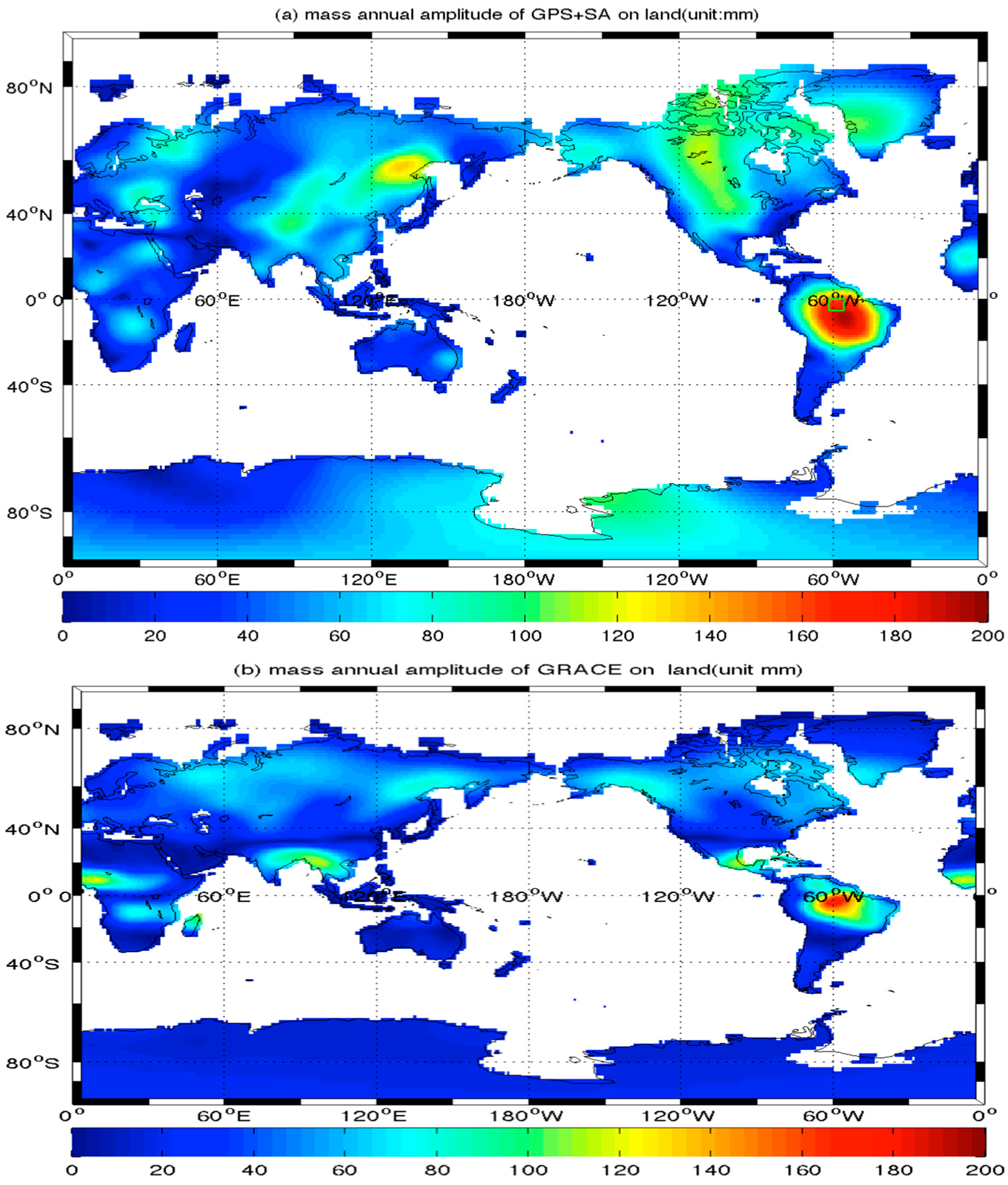
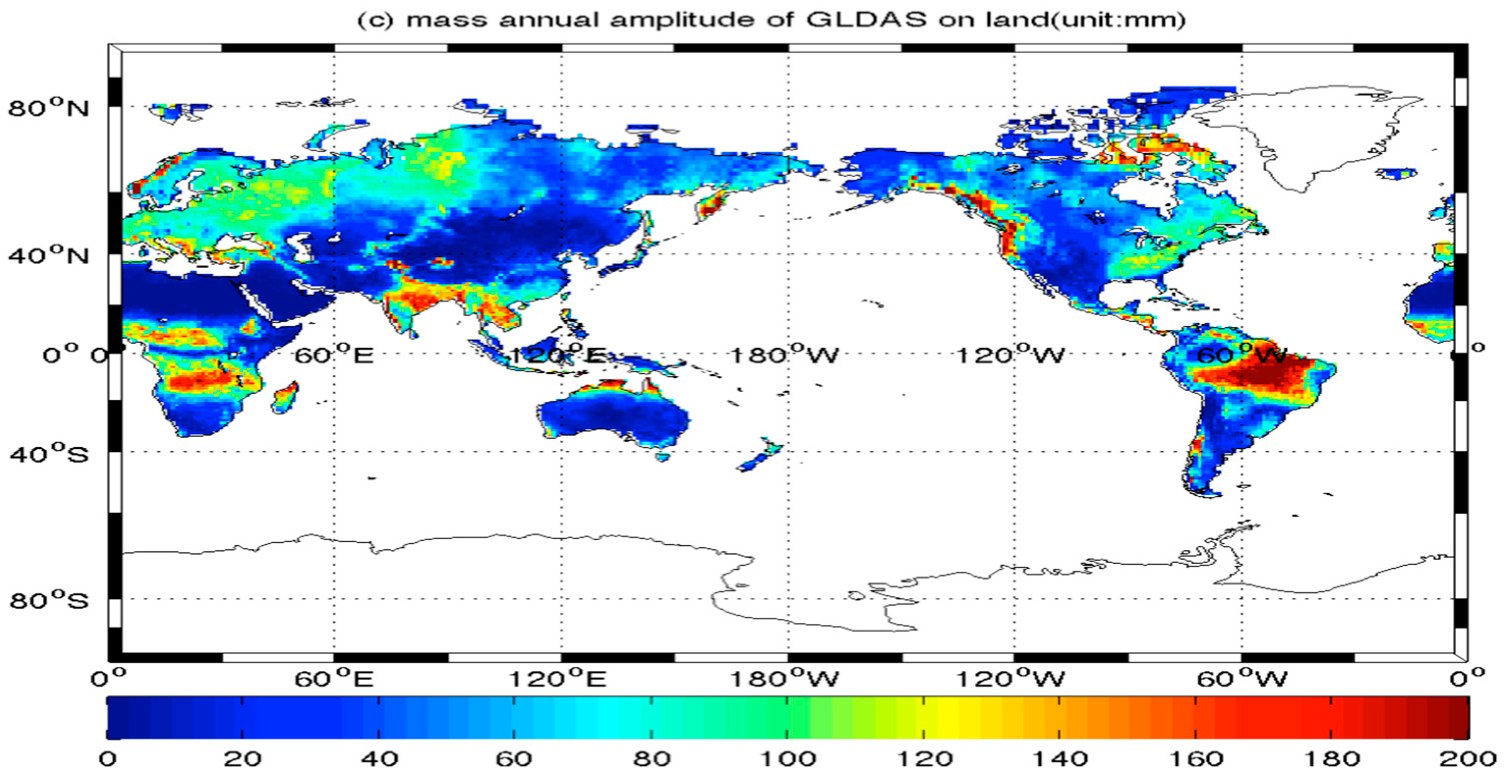
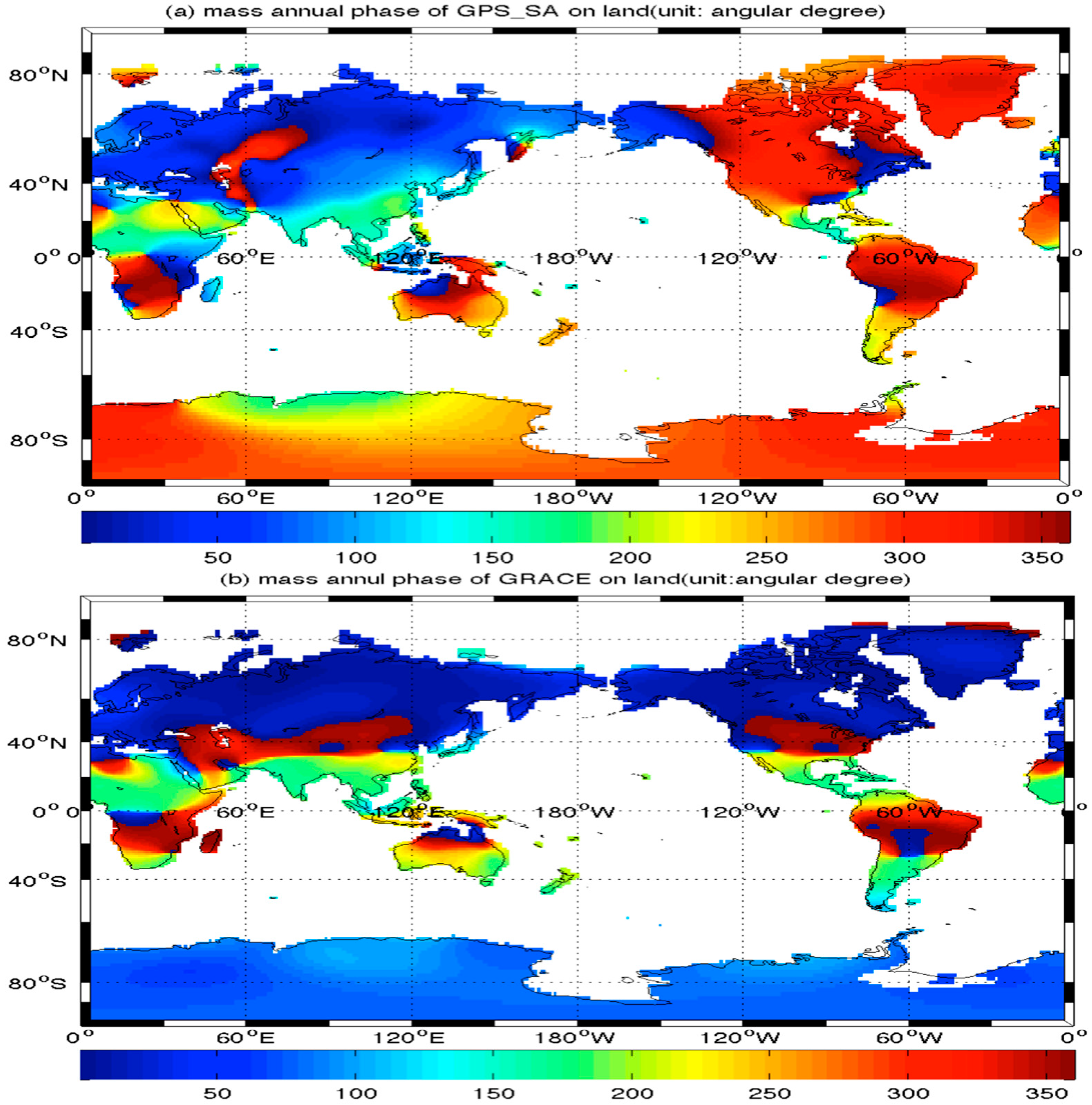
Figure 7a,c show annual amplitudes of terrestrial water storage of GPS+SA and GRACE and GLDAS (unit: mm) respectively. We find that (1) there is a significant annual cycle with about 200 mm amplitude in Amazon for GPS+SA, GRACE and GLDAS. Furthermore, GPS+SA reveals a wider area in Amazon than GRACE; (2) GPS+SA clearly detects a large mass signal in the mid zone of Europe and North America because of a denser GPS network over these two areas, especially in the middle of North America; (3) Both GPS+SA and GRACE find a strong signal on Greenland. Annual amplitudes observed by GPS+SA are stronger than GRACE in this region; (4) GRACE and GLDAS show a clear variation in annual water storage over south India. In contrast, the annual signal of GPS+SA is very weak because of fewer GPS sites in this region; (5) All three techniques show similar spatial patterns over Africa. The amplitudes derived from GPS+SA are weakest due to the sparse distribution of GPS sites; GLDAS is strongest; (6) GPS+SA also shows remarkable annual changes of water storage in east-north China. On the other hand, TWSs detected by GLDAS and GRACE are trivial. Figure 8 shows annual phases of land water storage. Their phases are consistent with each other and there is not much difference between them in most areas except in Greenland and part of Antarctica. Given that the uncertainty of GPS+SA (refer to Section 3.2.4) is about 53 mm using a 500 km Gaussian filter, the water storage estimates of GPS+SA in the Amazon are dependable. In other places, such as in Greenland, the mid-zone of Europe, North America and east-north China, the TWSs of GPS+SA might be just noise.
3.2.3. Annual Water Cycle in Amazon
The Amazon basin is the largest flood plain of tropical rainforest climate in the world. It is also the biggest rainy area near to the equator and has the widest Amazon River with the biggest water flow in the world. Therefore, there is a clear hydrological signal. To investigate the seasonal terrestrial water storage in the Amazon, we draw time series of TWS at point (58.50°W, 3.50°S) in the Amazon (Figure 9). The time series of GPS+SA, GRACE and GLDAS at this point are consistent with each other. Furthermore, GPS+SA has the largest magnitude.
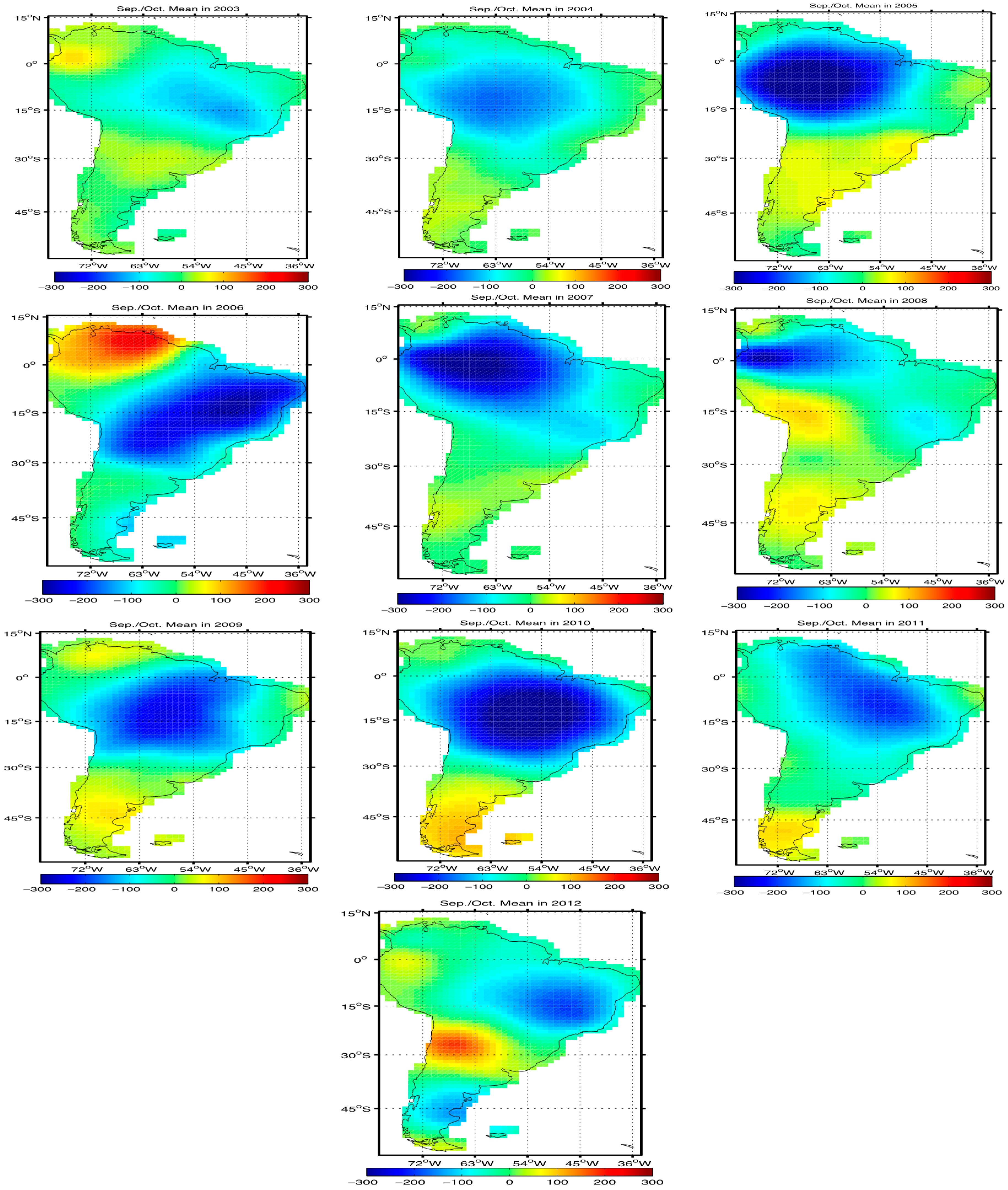
Because it is a dry period in September and October in the Amazon, we compute average TWS changes (unit: mm) in September and October from 2003 to 2012 using GPS+SA, GRACE and GLDAS to investigate the water reduction in these two months (Figure 10, Figure 11 and Figure 12). It shows that the TWS reduces by about 300 mm in a very dry year, and that the water reduction detected by GPS+SA and GRACE is much more significant than that detected by GLDAS. The inter-annual variation of GLDAS TWS is not more evident than GPS+SA and GRACE, which both detect severe drought in 2005 and 2010.
3.2.4. Estimation of Mass Error
Let , and represent errors in the mass and in the Stoke’s coefficients at epoch (). Applying error propagation and ignoring correlations between different Stoke’s coefficients, results in [40]:
where and are kernel average function, independent of time.
Following the method in [40], and can be viewed as the RMS of residuals of Stoke’s coefficients by removing the linear trend, constant bias, and annual cycle from monthly values of each Stoke’s coefficient. We also remove the semi-annual cycle to reduce the influence of the high frequency signal.
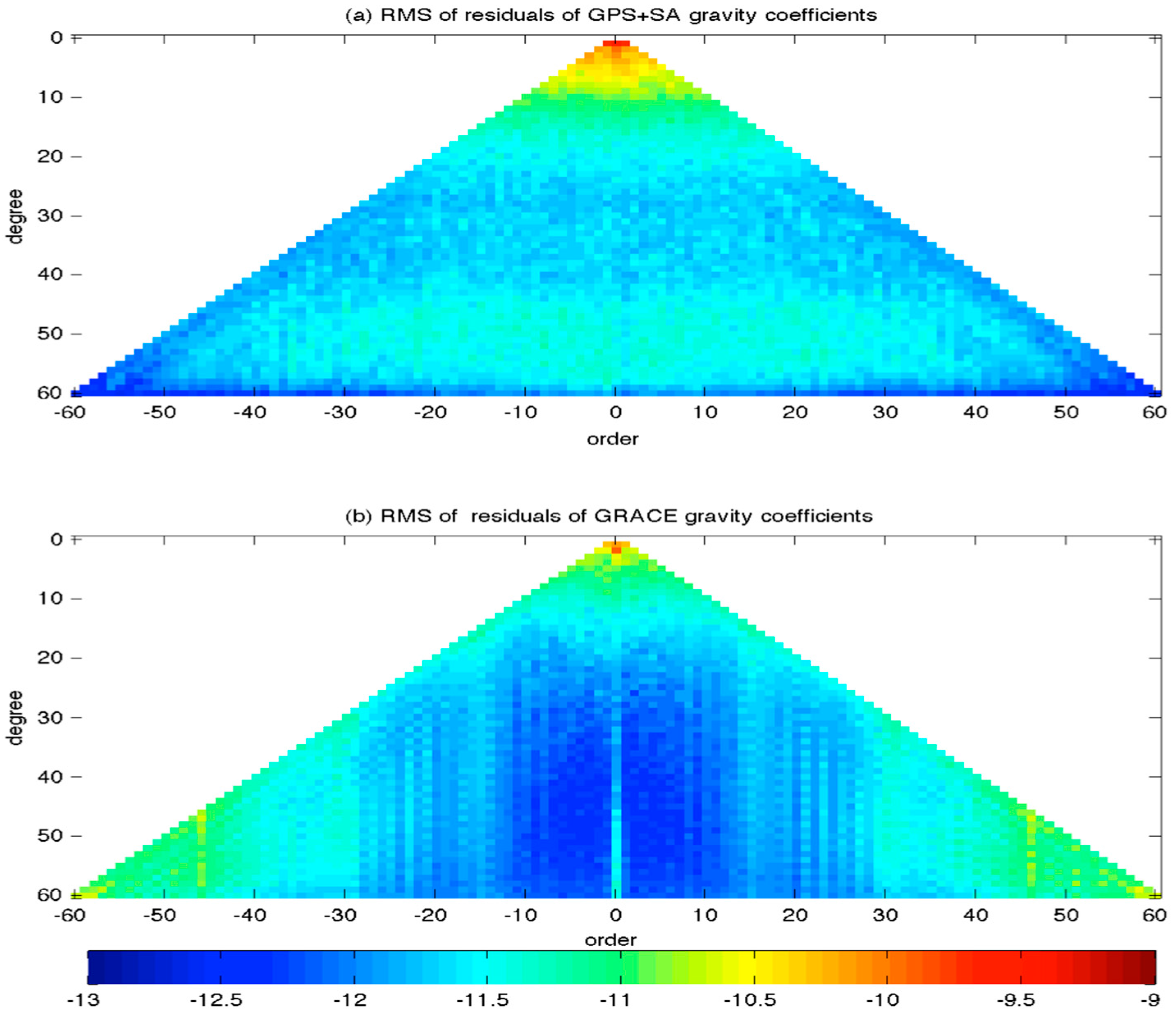
Figure 13 shows the logarithm of and of GPS+SA (top) and GRACE (bottom). The vertical axis represents degree n. The horizontal axis represents order m, m < 0 for SINE coefficients and m > 0 for COSINE coefficients. RMSs of degree 1–15 coefficients derived from GPS+SA are more remarkable than those of GRACE. RMSs of degree 1–5 coefficients of GPS+SA are larger than the rest. RMSs of GRACE are only outstanding in degree 1 and 2. For GRACE, the coefficients of order >29 are noisier than those of order <29 and degree < 20. Because of SA regularization, uncertainties of GPS+SA coefficients of order >29 are much less than corresponding GRACE coefficients.
Furthermore, we can assess the mass error from uncertainties of Stoke’s coefficients (Figure 14). Figure 14a shows the GPS+SA mass error with global mean 53.99 mm when atmosphere and ocean are not removed using the GRACE GAC product. Figure 14b is the GPS+SA mass error without atmosphere and sea. The global average is 53.36 mm. We can see that the effects of atmosphere and the sea on the mass error are trivial and mainly concentrated in low and mid-latitudes zone. Figure 14c is the GRACE mass error with atmosphere and sea. Its global average is 25.50 mm. Figure 14d is the GRACE mass error with atmosphere and sea removed. Its global average is 22.27 mm. The RMS of atmosphere and sea is just several millimeters. The GRACE error is 1–2 times less than that of GPS+SA.
3.3. Sensitivity Analysis
The contribution of each type of data set to our joining inversion pertains not only to measurement errors but also their coverage over the globe. Based on the least-squares theory, the measurement errors are represented as a stochastic model and the coverage information is contained in the design matrix of observation equations. As a result, the normal matrix of each data reflects the comprehensive effects of both the errors and data spatial distribution on final estimates.
Specifically, because our data sets are independent of each other, the contribution of each data set to the normal matrix can be computed:
where are the normal matrix from the data set of GPS site displacements, the data set of satellite altimetry and a priori constraints, respectively. is the total normal matrix.
The contribution of each data set to each Stoke’s coefficients can be considered as [41]:
where diag() means the diagonal elements of the matrix.
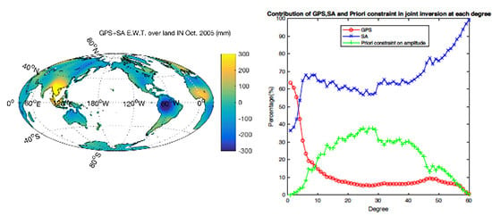
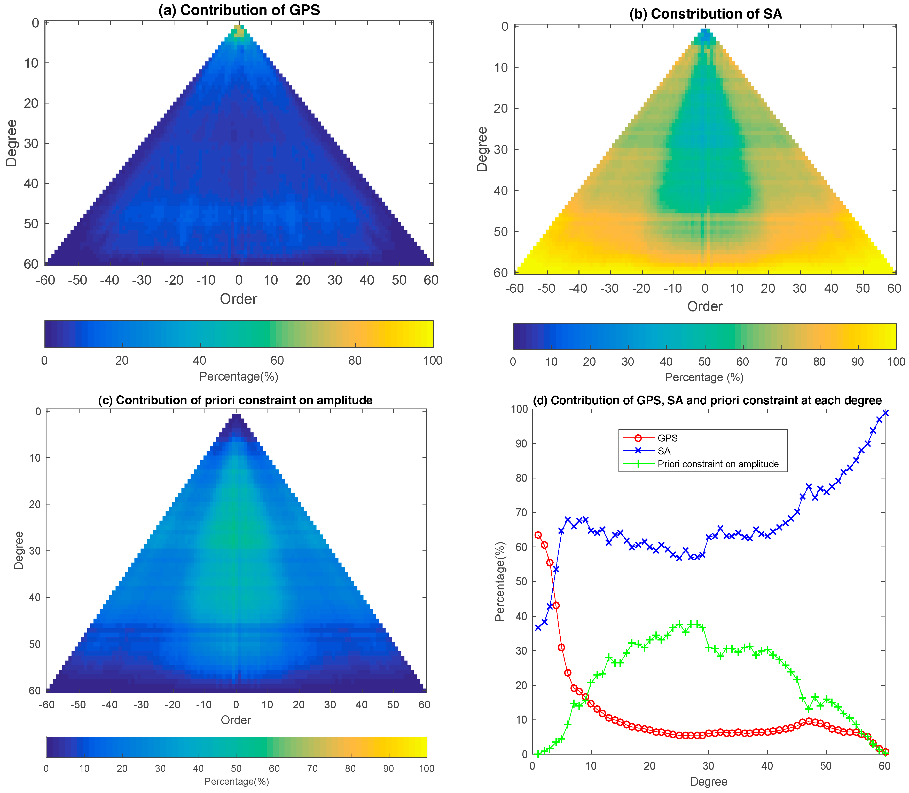
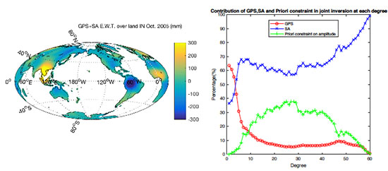
It was found that the GPS data contributes approximately more than 48% to low degree coefficients from degree 1 to degree 3 (Figure 15a,d), then its power decreases rapidly to 10%. This is due to the decreasing control power of the Load love number with increasing degree, and partly due to the insufficient spatial resolution of the GPS network.
What is impressive is that satellite altimetry acts as an effective complement to GPS (Figure 15 a,b,d). For example, GPS provides 48%, 70% and 73% power in X, Y and Z directions respectively. In contrast, SA contributes 52%, 30% and 27% to the X, Y and Z components respectively. This can possibly explain why the amplitude in the X direction of the geocenter is much less (Table 1), because the GPS signal is much stronger on the continent than the SA signal over the ocean, but its contribution is only 48% in our joint inversion. Furthermore, if we use only GPS to estimate the geocenter, meaning that GPS contribution is 100%, the annual amplitude of the X component can reach 1.42 cm [42].
The contribution of SA to C(2,0), C(2,1), S(2,1), C(2,2) and S(2,2) is only 28%, 28%, 46%, 43% and 44% respectively. The primary influence of SA lies at a degree higher than five, contributing about 60% (Figure 15d). The contribution of GPS measurements to the combination is almost zero at the highest degree, whereas SA impact becomes most significant, having almost 100% contribution. As a result, GPS actually determines the coefficients from degree one to degree three. The regularization from SA has a big impact on coefficients beyond degree 4 and improves their estimates.
The triangle shapes in the center of Figure 15b,c show another complement between SA and a priori constraint on amplitudes of Stoke’s coefficients at degree 10 to degree 45, where GPS contribution is limited. Furthermore, when order is equal to degree, SA power is most powerful while a priori constraint power is lowest.
4. Conclusions
In this paper, we have developed a joint inversion for the time-varying gravity field from 2003 to 2012, in which GPS and steric-corrected satellite altimeter data are merged. Our independently estimated Stoke’s coefficients include a full array of spherical harmonics up to degree and order 60 with a monthly solution. Comparing with GRACE, we can simultaneously estimate geocenter motion and higher-degree coefficients.
Two issues must be considered in the merging process. Firstly, although introducing SA data over the sea gives us almost global data coverage, it is still not sufficient to invert Stoke’s coefficients up to a higher degree because the linear system of observation equations becomes unstable and results in too large amplitudes of higher-degree Stoke’s coefficients from the ordinary least-square solution. To have reasonable amplitudes of Stoke’s coefficients, we introduced degree variances as a constraint. Secondly, data weighting for SA in joint inversion remains a difficult issue. We weighted SA with the sample variance of sea level anomalies.
The annual amplitudes of geocenter motion of our estimates are 0.81 mm, 1.79 mm and 2.29 mm in X, Y and Z components, respectively. Amplitude in the X component of our result is less than that of SLR [9] and that estimated by combining GRACE and the ocean model [38], which are denoted as GRACE, probably due to the fact that although the GPS signal is stronger than that of SA, GPS contributes only 48% in the X direction, in comparison with 70% and 73% in Y and Z directions respectively, when combining with SA. The phases between three kinds of geocenter are consistent with each other.
Comparing higher-degree Stoke’s coefficients, we find that the seasonal signals of C(2,0), C(2,1), C(2,2), S(2,2) of our results agree well with those of SLR and GRACE except that the annual phase of C(2,1) deviates much from SLR and GRACE, possibly because of the distribution of GPS stations. The magnitudes of other Stoke’s coefficients (degree > 2) of our estimates match those of GARCE, and some time series of our higher Stoke’s coefficients are more stable than those of GRACE. In addition, our estimated zonal Stoke’s coefficients (degree 15) agree well with those of GRACE.
To further validate our methodology, we investigated global large-scale mass redistributions using the inverted time-varying gravity field. Our results show that the combination of GPS and SA data can successfully and independently detect global large-scale mass changes, especially in the Amazon region, and the results agree well with those of GRACE observations and the GLDAS model. Our results also clearly reveal the drought (reduced by about 300 mm) in the Amazon in September and October. The mass uncertainty of our solution is about two times larger than that of GRACE using a 500 km Gaussian filter. Because of the spatial coverage, the GPS+SA and GLDAS models lack the ability to match GRACE fields. GRACE is the only method that provides us a global solution. The complementary function of GPS at low degree and SA at high degree is obvious through sensitivity analysis. If inverting the time-varying gravity field before 2002, our method might have some limitations because the GPS network is sparser at that time.
As mentioned before, the mass signal on land is much stronger than that over the sea, and a high quality GNSS time series is the key to our solution and must be carefully considered. Because we cannot separate the elastic long-term trend from the GPS time series, we could only investigate seasonal- and inter-annual mass redistribution. With the development of GPS data processing techniques, we may estimate secular global surface mass redistribution independently using only GNSS. Further, more other non-tectonics signals of GNSS observations will be further studied and removed in the future [43,44].
Acknowledgments
We thank the SOPAC, Aviso and Ishii for providing global time series, satellite altimeter data and steric variations in this work. We would like to thank Xiaoping Wu for his critical suggestions about how to correctly use JPL time series etc. We thank Wei Feng for his ideas and procedure to process satellite altimetry data. We would like to thank the anonymous reviewers and editors for their constructive reviews. Our research is also partly supported by the Chinese Academy of Sciences (CAS) program of “Light of West China” (Grant No. 29Y607YR000103), Chinese Academy of Sciences, Russia and Ukraine and other countries of special funds for scientific and technological cooperation (Grant No. 2BY711HZ000101), National Natural Science Foundation of China (NSFC) Project (Grant Nos. 11373059 and 61501430).
Author Contributions
Xinggang Zhang and Shuanggen Jin conceived and designed the experiments; Xinggang Zhang performed the experiment and analyzed the data; Xiaochun Lu contributed analysis tools; Xinggang Zhang wrote the paper.
Conflicts of Interest
The authors declare no conflict of interest.
Appendix A
This section shows the process to prove Equation (2).
The normalized associated Legendre functions in Equation (1) are [26]
having property
where is Kronecker delta which is one if , and zero elsewhere.
Let and be two vectors separated by the angle . Then, following the addition theorem, we have
where are Legendre polynomials.
If , it turns out that we can expand into spherical harmonics as:
Furthermore, suppose we know the mass density function at the point inside the earth. The potential energy at the point outside the earth can be expressed as:
When there is a surface density, concentrated on the spherical surface , Equation (A5) becomes:
where .
Substitute Equations (1), (A2) and (A3) into (A6) and use the orthogonality of spherical harmonics and the following simple expressions:
where g is surface acceleration due to gravity at the Earth’s surface, is the mass of the Earth and G is the gravitational constant. The incremental gravitational quantity at the surface of the Earth is obtained:
According to Loading Love number theory, the displacements of station in height and lateral direction are given by Equation (3) of article [26]:
where is the unit vector in lateral direction. is the surface gradient operator, in which and are unit vectors pointing northward and eastward, respectively.
In particular, let ,, and substituting Equation (A8) into Equation (A9), Equation (2) can be proved.
References
- Tapley, B.D.; Bettadpur, S.; Watkins, M.; Reigber, C. GRACE measurements of mass variability in the Earth system. Science 2004, 305, 503–505. [Google Scholar] [CrossRef] [PubMed]
- Chen, J.L.; Wilson, C.R.; Tapley, B.D. Satellite gravity measurements confirm accelerated melting of Greenland ice sheet. Science 2006, 313, 1958–1960. [Google Scholar] [CrossRef] [PubMed]
- Chen, J.L.; Wilson, C.R.; Tapley, B.D.; Famiglietti, J.S.; Rodell, M. Seasonal global mean sea level change from satellite altimeter, GRACE, and geophysical models. J. Geod. 2005, 79, 532–539. [Google Scholar] [CrossRef]
- Chen, J.L.; Rodell, M.; Wilson, C.R.; Famiglietti, J.S. Low degree spherical harmonic influences on Gravity Recovery and Climate Experiment (GRACE) water storage estimates. Geophys. Res. Lett. 2005. [Google Scholar] [CrossRef]
- Chen, J.L.; Wilson, C.R.; Tapley, B.D. Interannual variability of low-degree gravitational change, 1980–2002. J. Geod. 2005, 78, 535–543. [Google Scholar] [CrossRef]
- Chen, J.L.; Wilson, C.R.; Tapley, B.D.; Yang, Z.L.; Niu, G.Y. 2005 drought event in the Amazon River basin as measured by GRACE and estimated by climate models. J. Geophys. Res. Solid Earth 2009. [Google Scholar] [CrossRef]
- Chen, J.L.; Wilson, C.R.; Tapley, B.D. The 2009 exceptional Amazon flood and interannual terrestrial water storage change observed by GRACE. Water Resour. Res. 2010, 46. [Google Scholar] [CrossRef]
- Cheng, M.; Tapley, B.D. Variations in the Earth’s oblateness during the past 28 years. J. Geophys. Res. Solid Earth 2004. [Google Scholar] [CrossRef]
- Cheng, M.K.; Ries, J.C.; Tapley, B.D. Geocenter variations from analysis of SLR data. In Reference Frames for Applications in Geosciences; Springer: Berlin/Heidelberg, Germany, 2013; pp. 19–25. [Google Scholar]
- Cheng, M.; Ries, J.C.; Tapley, B.D. Variations of the Earth’s figure axis from satellite laser ranging and GRACE. J. Geophys. Res. Solid Earth 2011. [Google Scholar] [CrossRef]
- Cheng, M.; Tapley, B.D.; Ries, J.C. Deceleration in the Earth’s oblateness. J. Geophys. Res. 2013, 118, 740–747. [Google Scholar] [CrossRef]
- Sośnica, K.; Jäggi, A.; Meyer, U.; Thaller, D.; Beutler, G.; Arnold, D.; Dach, R. Time variable Earth’s gravity field from SLR satellites. J. Geod. 2015, 89, 945–960. [Google Scholar] [CrossRef] [Green Version]
- Kang, Z.; Tapley, B.; Chen, J.; Ries, J.; Bettadpur, S. Geocenter variations derived from GPS tracking of the GRACE satellites. J. Geod. 2009, 83, 895–901. [Google Scholar] [CrossRef]
- Lin, T.; Hwang, C.; Tseng, T.P.; Chao, B.F. Low-degree gravity change from GPS data of COSMIC and GRACE satellite missions. J. Geodyn. 2012, 53, 34–42. [Google Scholar] [CrossRef]
- Wang, X.; Gerlach, C.; Rummel, R. Time-variable gravity field from satellite constellations using the energy integral. Geophys. J. Int. 2012, 190, 1507–1525. [Google Scholar] [CrossRef]
- Rodell, M.; Velicogna, I.; Famiglietti, J.S. Satellite-based estimates of groundwater depletion in India. Nature 2009, 460, 999–1002. [Google Scholar] [CrossRef] [PubMed]
- Blewitt, G.; Lavallée, D.; Clarke, P.; Nurutdinov, K. A new global mode of Earth deformation: Seasonal cycle detected. Science 2001, 294, 2342–2345. [Google Scholar] [CrossRef] [PubMed]
- Wu, X.; Argus, D.F.; Heflin, M.B.; Ivins, E.R.; Webb, F.H. Site distribution and aliasing effects in the inversion for load coefficients and geocenter motion from GPS data. Geophys. Res. Lett. 2002. [Google Scholar] [CrossRef]
- Lavallée, D.A.; Van Dam, T.; Blewitt, G.; Clarke, P.J. Geocenter motions from GPS: A unified observation model. J. Geophys. Res. Solid Earth 2006. [Google Scholar] [CrossRef]
- Kusche, J.E.J.O.; Schrama, E.J.O. Surface mass redistribution inversion from global GPS deformation and Gravity Recovery and Climate Experiment (GRACE) gravity data. J. Geophys. Res. Solid Earth 2005. [Google Scholar] [CrossRef]
- Rietbroek, R.; Brunnabend, S.E.; Dahle, C.; Kusche, J.; Flechtner, F.; Schröter, J.; Timmermann, R. Changes in total ocean mass derived from GRACE, GPS, and ocean modeling with weekly resolution. J. Geophys. Res. Oceans 2009. [Google Scholar] [CrossRef]
- Rietbroek, R.; Fritsche, M.; Dahle, C.; Brunnabend, S.E.; Behnisch, M.; Kusche, J.; Dietrich, R. Can GPS-Derived Surface Loading Bridge a GRACE Mission Gap? Surv. Geophys. 2014, 35, 1267–1283. [Google Scholar] [CrossRef]
- Siegismund, F.; Romanova, V.; Köhl, A.; Stammer, D. Ocean bottom pressure variations estimated from gravity, nonsteric sea surface height and hydrodynamic model simulations. J. Geophys. Res. Oceans 2011. [Google Scholar] [CrossRef]
- Wu, X.; Heflin, M.B.; Ivins, E.R.; Fukumori, I. Seasonal and interannual global surface mass variations from multisatellite geodetic data. J. Geophys. Res. Solid Earth 2006. [Google Scholar] [CrossRef]
- Wu, X.; Heflin, M.B.; Schotman, H.; Vermeersen, B.L.; Dong, D.; Gross, R.S.; Owen, S.E. Simultaneous estimation of global present-day water transport and glacial isostatic adjustment. Nat. Geosci. 2010, 3, 642–646. [Google Scholar] [CrossRef]
- Wahr, J.; Molenaar, M.; Bryan, F. Time variability of the Earth’s gravity field: Hydrological and oceanic effects and their possible detection using GRACE. J. Geophys. Res. Solid Earth 1998, 103, 30205–30229. [Google Scholar] [CrossRef]
- Blewitt, G. Self-consistency in reference frames, geocenter definition, and surface loading of the solid Earth. J. Geophys. Res. Solid Earth 2003. [Google Scholar] [CrossRef]
- Kedar, S.; Bock, Y.; Moore, A.W.; Squibb, M.B.; Liu, Z.; Hasse, J.; Fang, P. Solid Earth Science ESDR System. In Proceedings of the 2013 American Geophysical Union (AGU) Fall Meeting, San Francisco, CA, USA, 9–13 December 2013; Available online: http://adsabs.harvard.edu/abs/2013AGUFM.G23C..08K (accessed on 5 August 2017).
- Mao, A.; Harrison, C.G.; Dixon, T.H. Noise in GPS coordinate time series. J. Geophys. Res. Solid Earth 1999, 104, 2797–2816. [Google Scholar] [CrossRef]
- Zhang, J.; Bock, Y.; Johnson, H.; Fang, P.; Williams, S.; Genrich, J.; Wdowinski, S.; Behr, J. Southern California Permanent GPS Geodetic Array: Error analysis of daily position estimates and site velocities. J. Geophys. Res. Solid Earth 1997, 102, 18035–18055. [Google Scholar] [CrossRef]
- Jayne, S.R.; Wahr, J.M.; Bryan, F.O. Observing ocean heat content using satellite gravity and altimetry. J. Geophys. Res. Oceans 2003. [Google Scholar] [CrossRef]
- Leuliette, E.W.; Miller, L. Closing the sea level rise budget with altimetry, Argo, and GRACE. Geophys. Res. Lett. 2009. [Google Scholar] [CrossRef]
- Blewitt, G.; Clarke, P. Inversion of Earth’s changing shape to weigh sea level in static equilibrium with surface mass redistribution. J. Geophys. Res. Solid Earth 2003. [Google Scholar] [CrossRef]
- Bettadpur, S. Level-2 Gravity Field Product User Handbook. Available online: http://csrserv.csr.utexas.edu/grace/publications/handbook/L2-UserHandbook_v1.0.pdf (accessed on 5 August 2017).
- Ishii, M.; Kimoto, M. Reevaluation of historical ocean heat content variations with time-varying XBT and MBT depth bias corrections. J. Oceanogr. 2009, 65, 287–299. [Google Scholar] [CrossRef]
- Ishii, M.; Kimoto, M.; Sakamoto, K.; Iwasaki, S.I. Steric sea level changes estimated from historical ocean subsurface temperature and salinity analyses. J. Oceanogr. 2006, 62, 155–170. [Google Scholar] [CrossRef]
- Zheng, D.W.; Zhong, P.; Ding, X.L.; Chen, W. Filtering GPS time-series using a Vondrak filter and cross-validation. J. Geod. 2005, 79, 363–369. [Google Scholar] [CrossRef]
- Swenson, S.; Chambers, D.; Wahr, J. Estimating geocenter variations from a combination of GRACE and ocean model output. J. Geophys. Res. Solid Earth 2008. [Google Scholar] [CrossRef]
- Chambers, D.P. Converting Release-04 Gravity Coefficients into Maps of Equivalent Water Thickness; University of Texas at Austin: Austin, TX, USA, 2007. [Google Scholar]
- Wahr, J.; Swenson, S.; Velicogna, I. Accuracy of GRACE mass estimates. Geophys. Res. Lett. 2006. [Google Scholar] [CrossRef]
- Jansen, M.J.F.; Gunter, B.C.; Kusche, J. The impact of GRACE, GPS and OBP data on estimates of global mass redistribution. Geophys. J. Int. 2009, 177, 1–13. [Google Scholar] [CrossRef]
- Zhang, X.; Jin, S. Uncertainties and effects on geocenter motion estimates from global GPS observations. Adv. Space Res. 2014, 54, 59–71. [Google Scholar] [CrossRef]
- Jin, S.G.; Luo, O.F.; Gleason, S. Characterization of diurnal cycles in ZTD from a decade of global GPS observations. J. Geodesy 2009, 83, 537–545. [Google Scholar] [CrossRef]
- Jin, S.G.; Zhang, T.; Zou, F. Glacial density and GIA in Alaska estimated from ICESat, GPS and GRACE measurements. J. Geophys. Res. Earth Surf. 2017, 122, 76–90. [Google Scholar] [CrossRef]
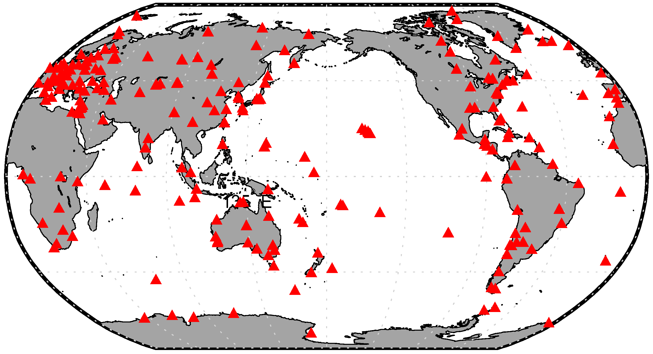
Figure 1.
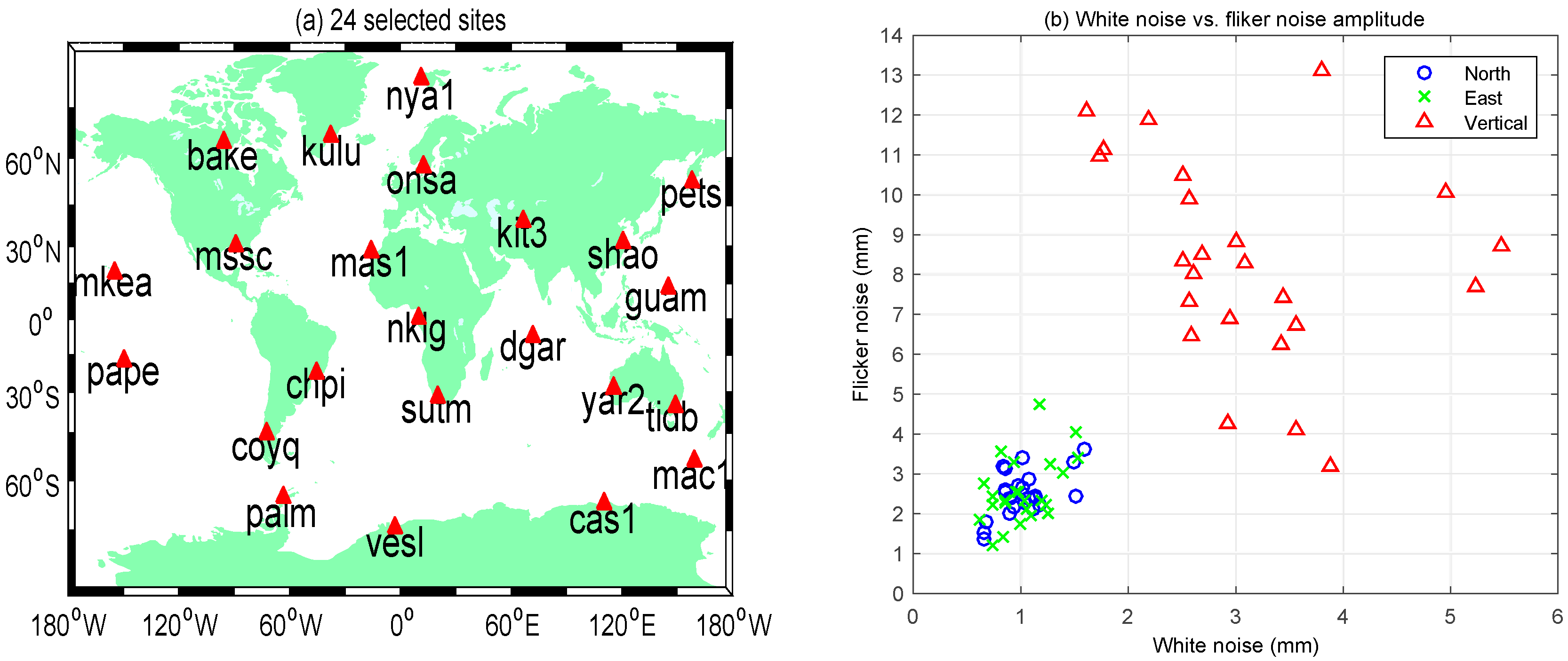
The 387 used GPS tracking sites (red triangles) selected from the ITRF2008 GPS network. Except for GPS ground observations, its stochastic model must be provided when we employ least-squares adjustments. Through the power spectral method and the maximum likelihood estimation method, several studies have recognized that the GPS time series was best described as a combination of white noise and flicker noise [29,30]. For simplicity, 24 global even distribution of stations among 387 GPS tracking sites are selected as examples to show the noise characteristics of GPS timeseries (Figure 2a,b). The magnitudes of flicker noise are about 2–5 times greater than those of white noise in all three directions. Furthermore, the noises in vertical directions are somewhat greater than in the horizontal direction.
Figure 1.
The 387 used GPS tracking sites (red triangles) selected from the ITRF2008 GPS network. Except for GPS ground observations, its stochastic model must be provided when we employ least-squares adjustments. Through the power spectral method and the maximum likelihood estimation method, several studies have recognized that the GPS time series was best described as a combination of white noise and flicker noise [29,30]. For simplicity, 24 global even distribution of stations among 387 GPS tracking sites are selected as examples to show the noise characteristics of GPS timeseries (Figure 2a,b). The magnitudes of flicker noise are about 2–5 times greater than those of white noise in all three directions. Furthermore, the noises in vertical directions are somewhat greater than in the horizontal direction.

Figure 2.
(a) The 24 global even distribution sites to show the noise characteristics of GPS time series; (b) White noise components and flicker noise components corresponding to 24 selected GPS sites.
Figure 2.
(a) The 24 global even distribution sites to show the noise characteristics of GPS time series; (b) White noise components and flicker noise components corresponding to 24 selected GPS sites.

Figure 3.
RMSs of the sea level anomaly (unit: m).
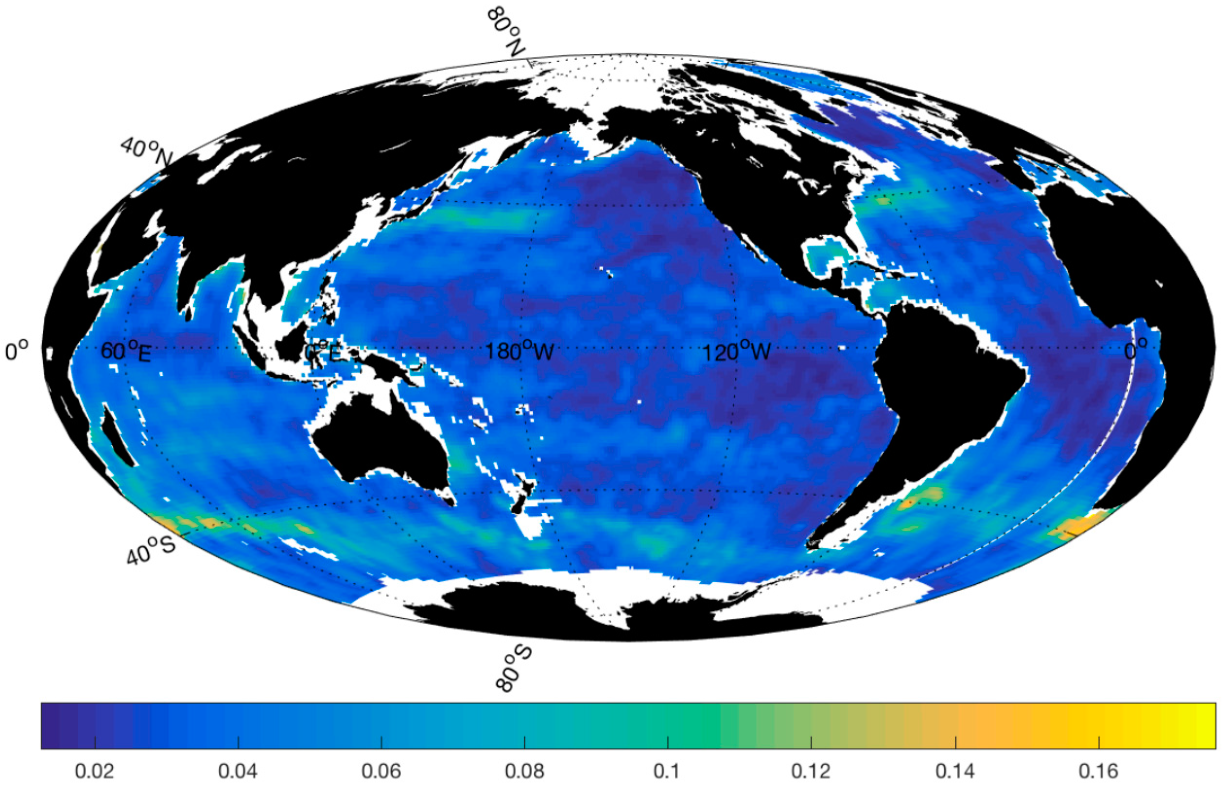
Figure 4.
Geocenter time series estimated from GPS+SA, SLR and GRACE. GPS+SA shows the results from combining GPS and SA. GRACE geocenter is computed by combining GRACE and the OBP model [38].
Figure 4.
Geocenter time series estimated from GPS+SA, SLR and GRACE. GPS+SA shows the results from combining GPS and SA. GRACE geocenter is computed by combining GRACE and the OBP model [38].
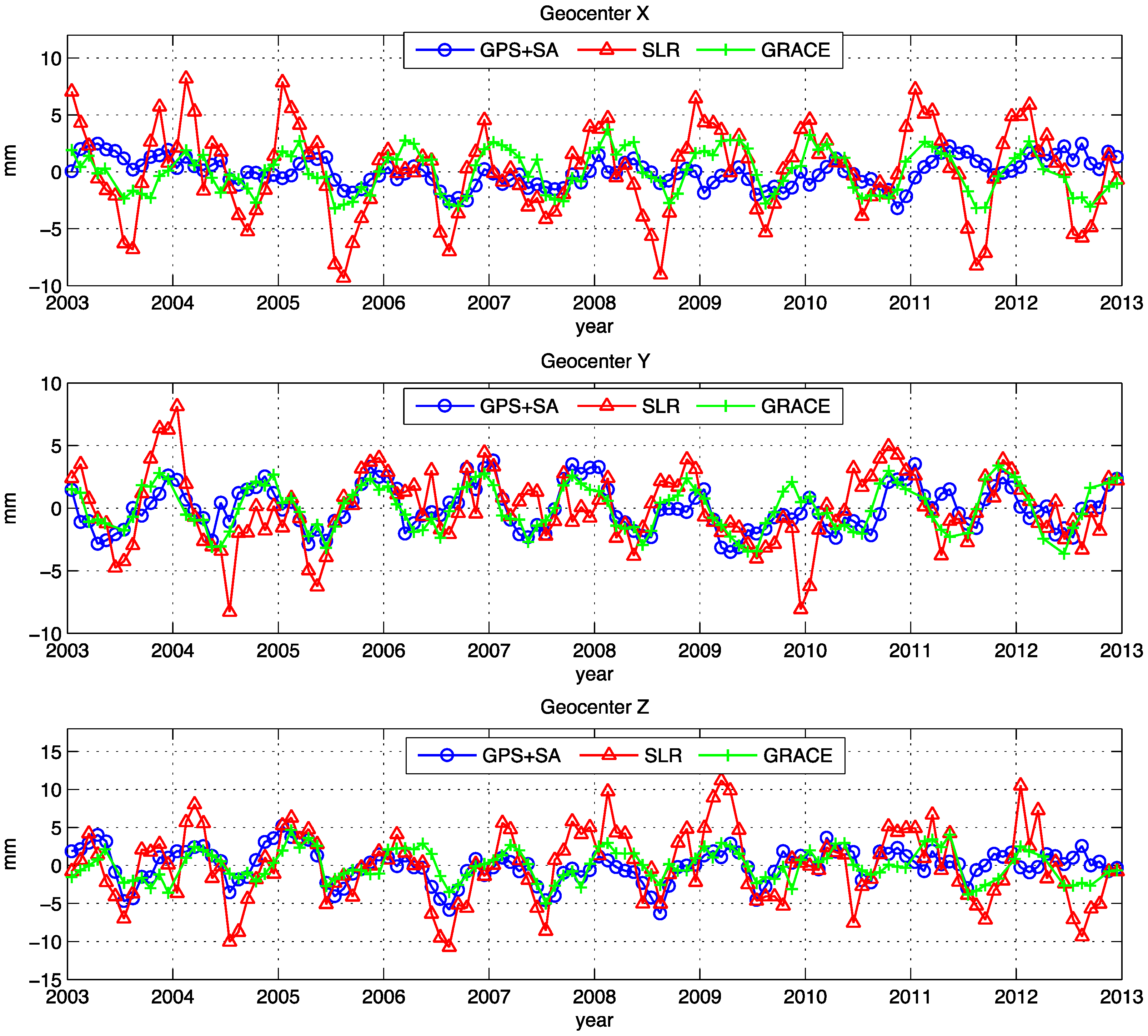
Figure 5.
Time series of time-varying degree-2 gravity coefficients estimated from GPS+SA, SLR and GRACE. GPS+SA shows the results from combining GPS and SA with the truncation degree at 60. GRACE results are from the CSR RL05 product. SLR results are from [9,10]. Figures from the top to bottom are time series of C20, C21, S21, C22 and S22 respectively.
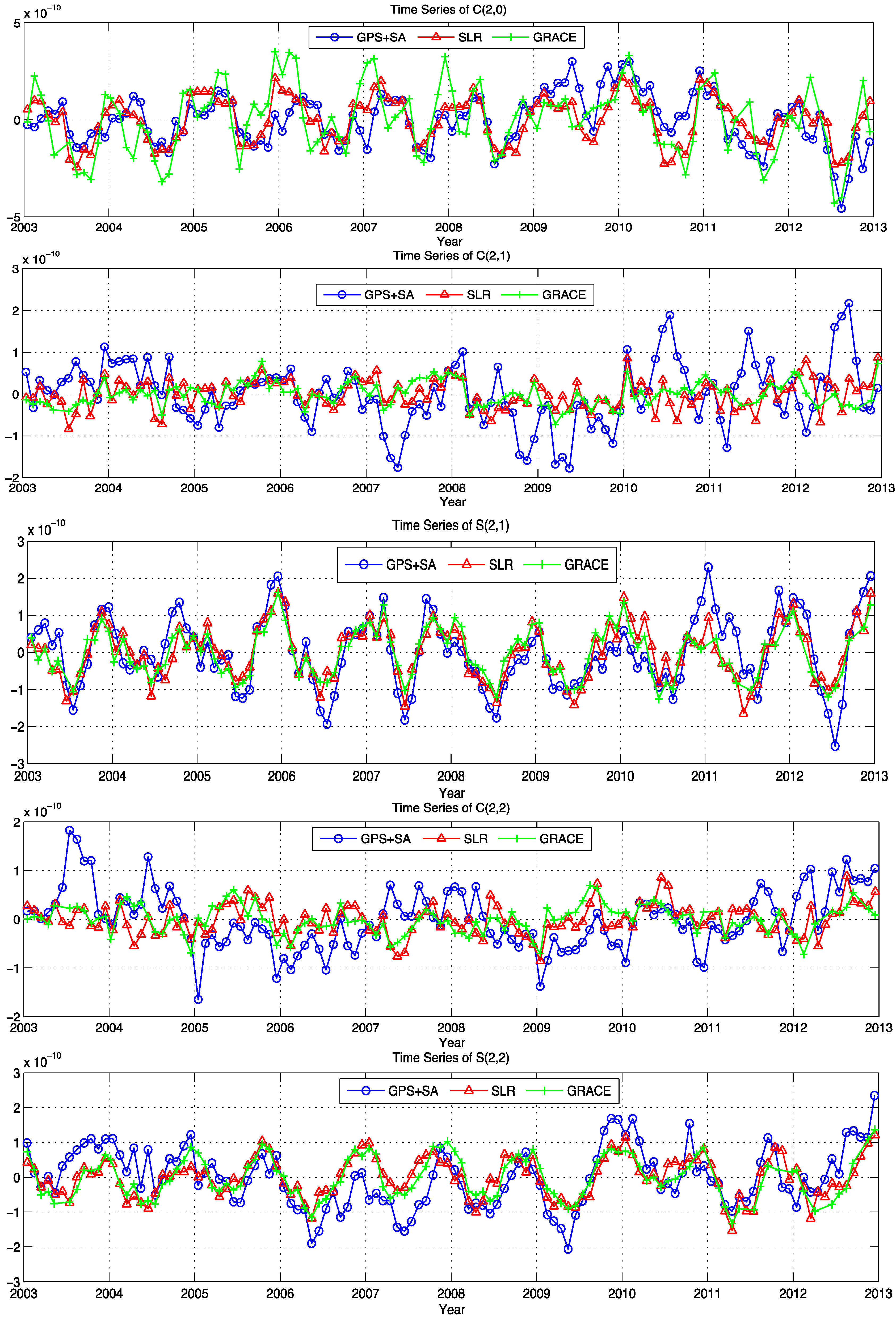
Figure 6.
Low-degree zonal Stoke’s coefficients estimated from GPS+SA and GRACE. Where GPS+SA shows results by combining GPS and SA the with truncation degree at 60. GRACE results are from CSR RL05 product.
Figure 6.
Low-degree zonal Stoke’s coefficients estimated from GPS+SA and GRACE. Where GPS+SA shows results by combining GPS and SA the with truncation degree at 60. GRACE results are from CSR RL05 product.
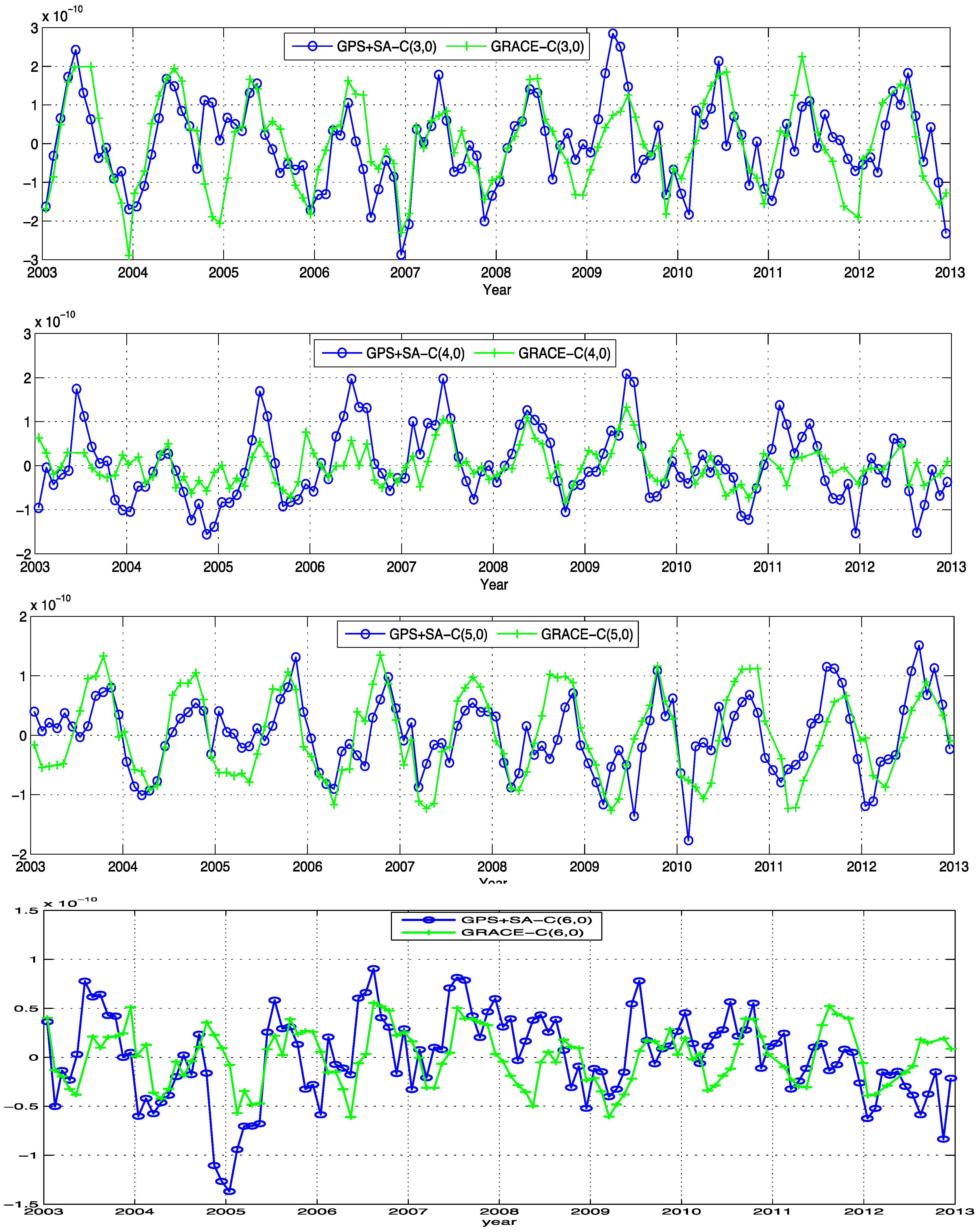
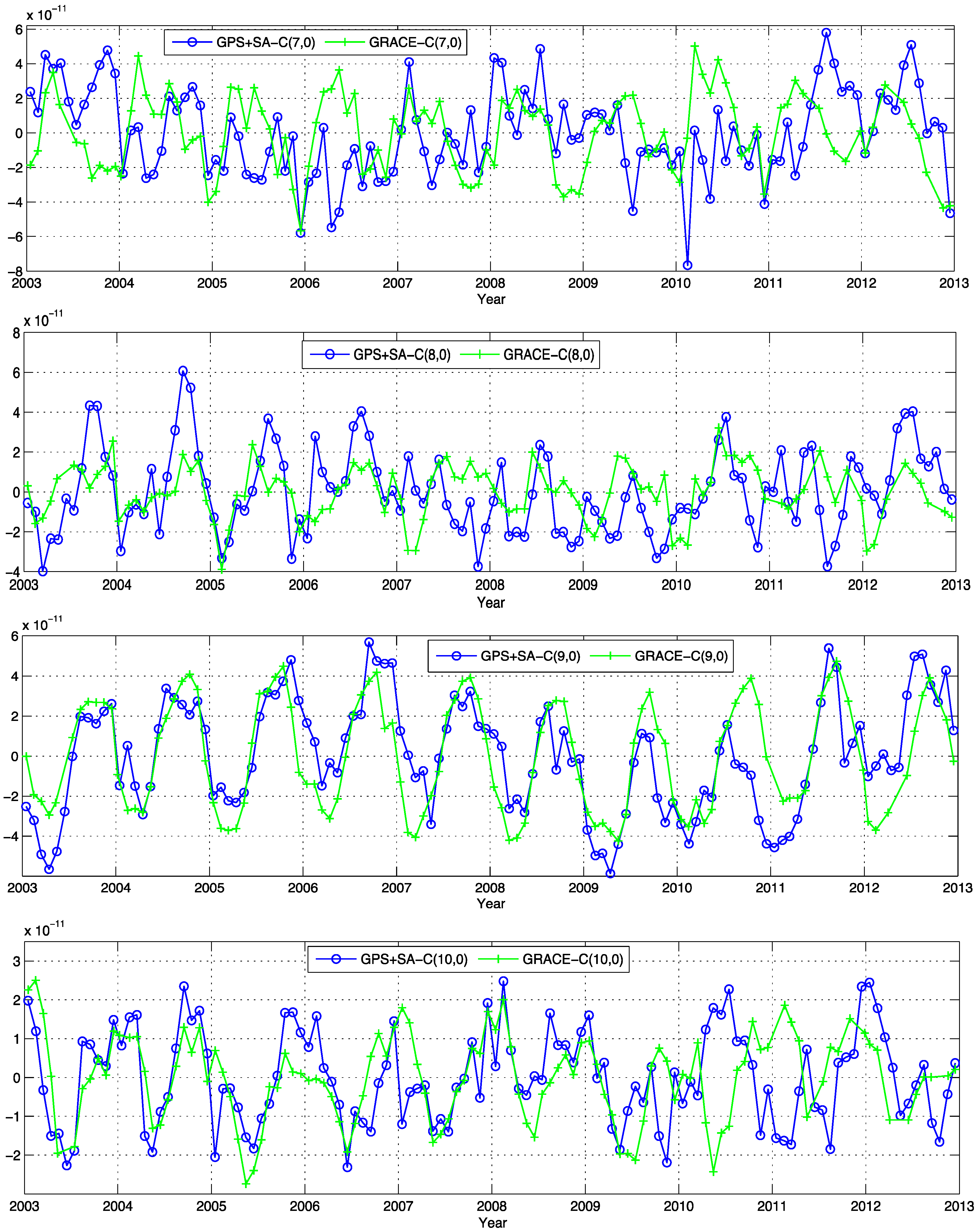
Figure 7.
Annual amplitudes of terrestrial water storage derived from GPS+SA and GRACE and GLDAS (unit: mm) using ten years of data from January 2003 to December 2012. For GPS+SA, atmosphere and sea mass variations are removed with GRACE in-situ products. (a–c) correspond to results of GPS+SA, GRACE RL05 and GLDAS respectively.


Figure 8.
Annual phases of terrestrial water storage of GPS+SA and GRACE and GLDAS (unit: mm) using ten years of data from 2003 to 2012. Atmosphere and ocean mass variations are removed with the GRACE in-situ product. (a–c) are results of GPS+SA, GRACE RL05 and GLDAS respectively.
Figure 8.
Annual phases of terrestrial water storage of GPS+SA and GRACE and GLDAS (unit: mm) using ten years of data from 2003 to 2012. Atmosphere and ocean mass variations are removed with the GRACE in-situ product. (a–c) are results of GPS+SA, GRACE RL05 and GLDAS respectively.

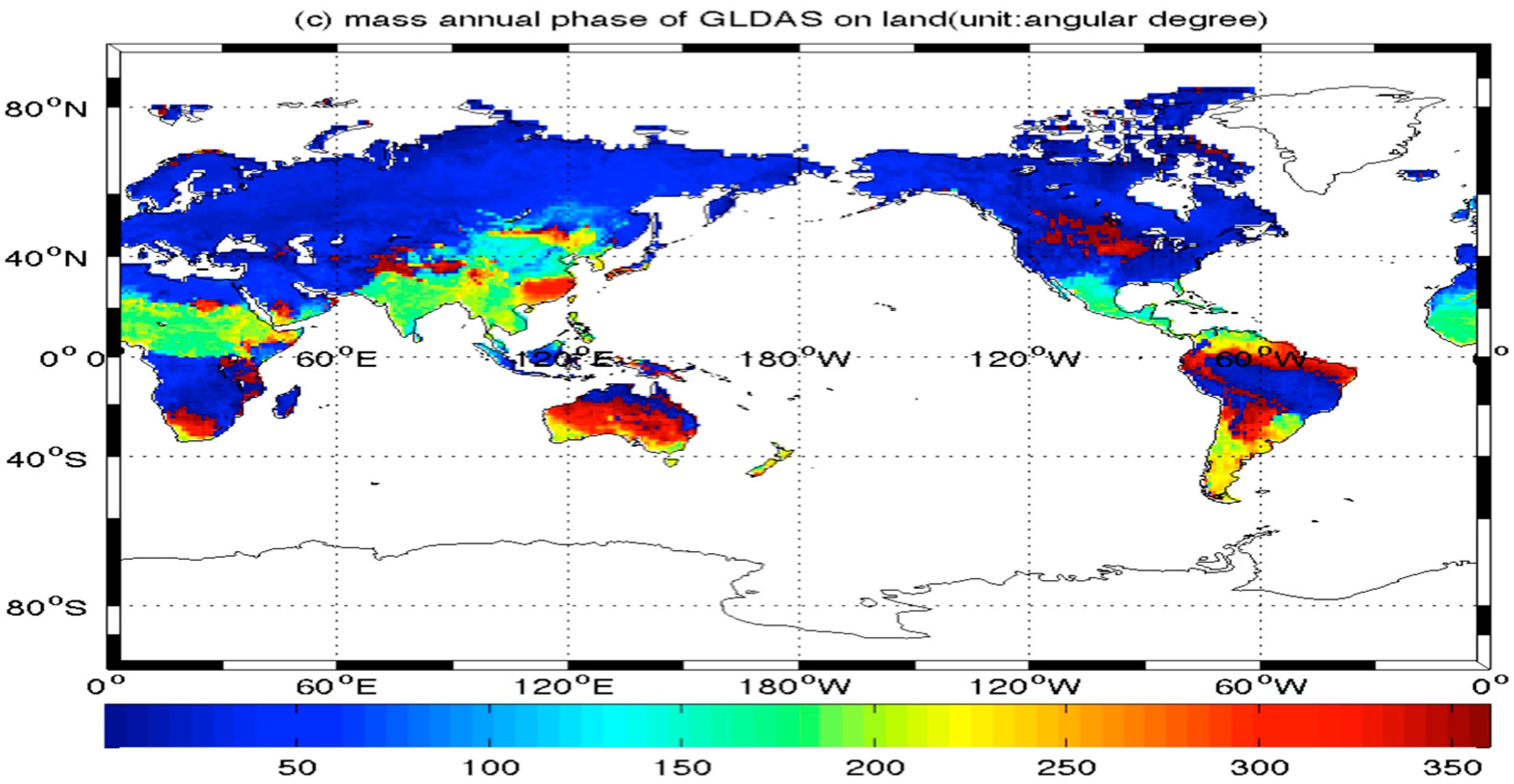
Figure 9.
Comparison of time series of terrestrial water storage (TWS) (unit: mm) at point (58.50°W, 3.50°S) in the Amazon between GPS+SA, GRACE and GLDAS.
Figure 9.
Comparison of time series of terrestrial water storage (TWS) (unit: mm) at point (58.50°W, 3.50°S) in the Amazon between GPS+SA, GRACE and GLDAS.
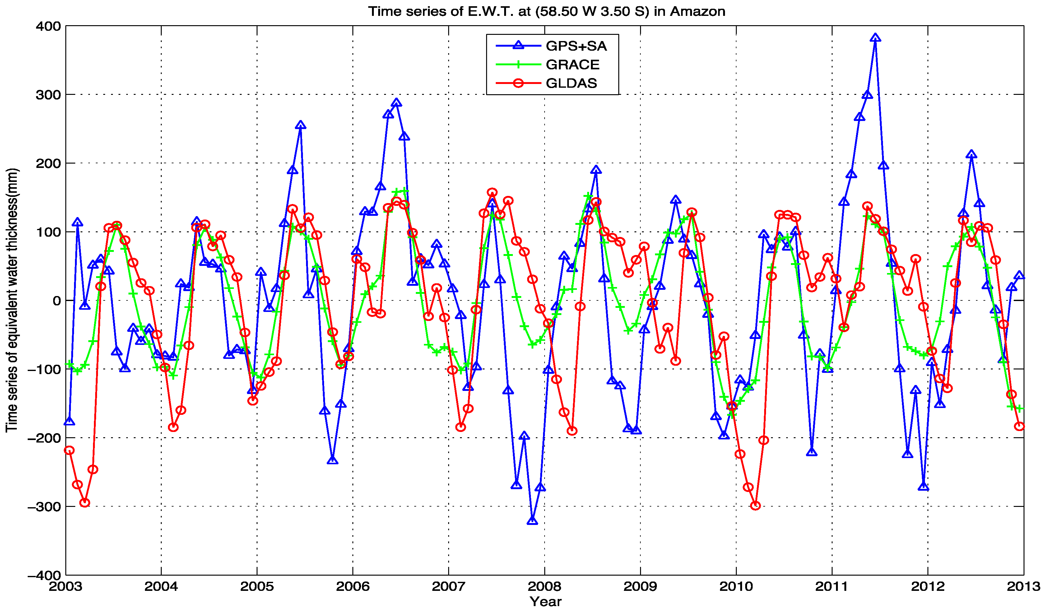
Figure 10.
GPS+SA-averaged September and October water storage changes (unit: mm) in the Amazon after a Gaussian filter with half wavelength is applied at 500 km. From left to right and from top to bottom are years from 2003 to 2012 successively.
Figure 10.
GPS+SA-averaged September and October water storage changes (unit: mm) in the Amazon after a Gaussian filter with half wavelength is applied at 500 km. From left to right and from top to bottom are years from 2003 to 2012 successively.

Figure 11.
GRACE-averaged September and October water storage changes (unit: mm) in the Amazon after a Gaussian filter with half wavelength is applied at 500 km. From left to right and from top to bottom are years from 2003 to 2012 successively.
Figure 11.
GRACE-averaged September and October water storage changes (unit: mm) in the Amazon after a Gaussian filter with half wavelength is applied at 500 km. From left to right and from top to bottom are years from 2003 to 2012 successively.
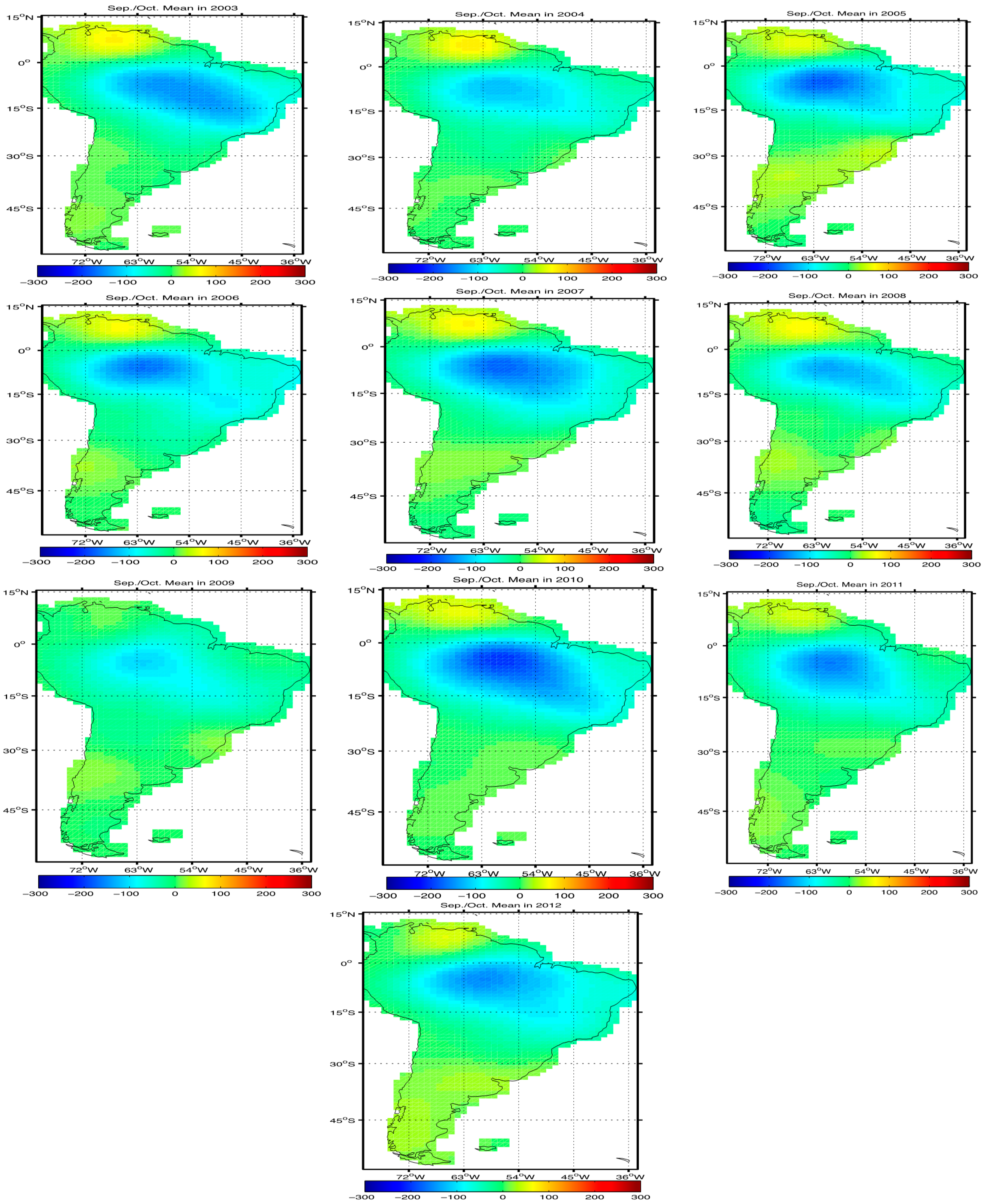
Figure 12.
GLDAS-averaged September and October water storage changes (unit: mm) in the Amazon. From left to right and from top to bottom are years from 2003 to 2012 successively.
Figure 12.
GLDAS-averaged September and October water storage changes (unit: mm) in the Amazon. From left to right and from top to bottom are years from 2003 to 2012 successively.
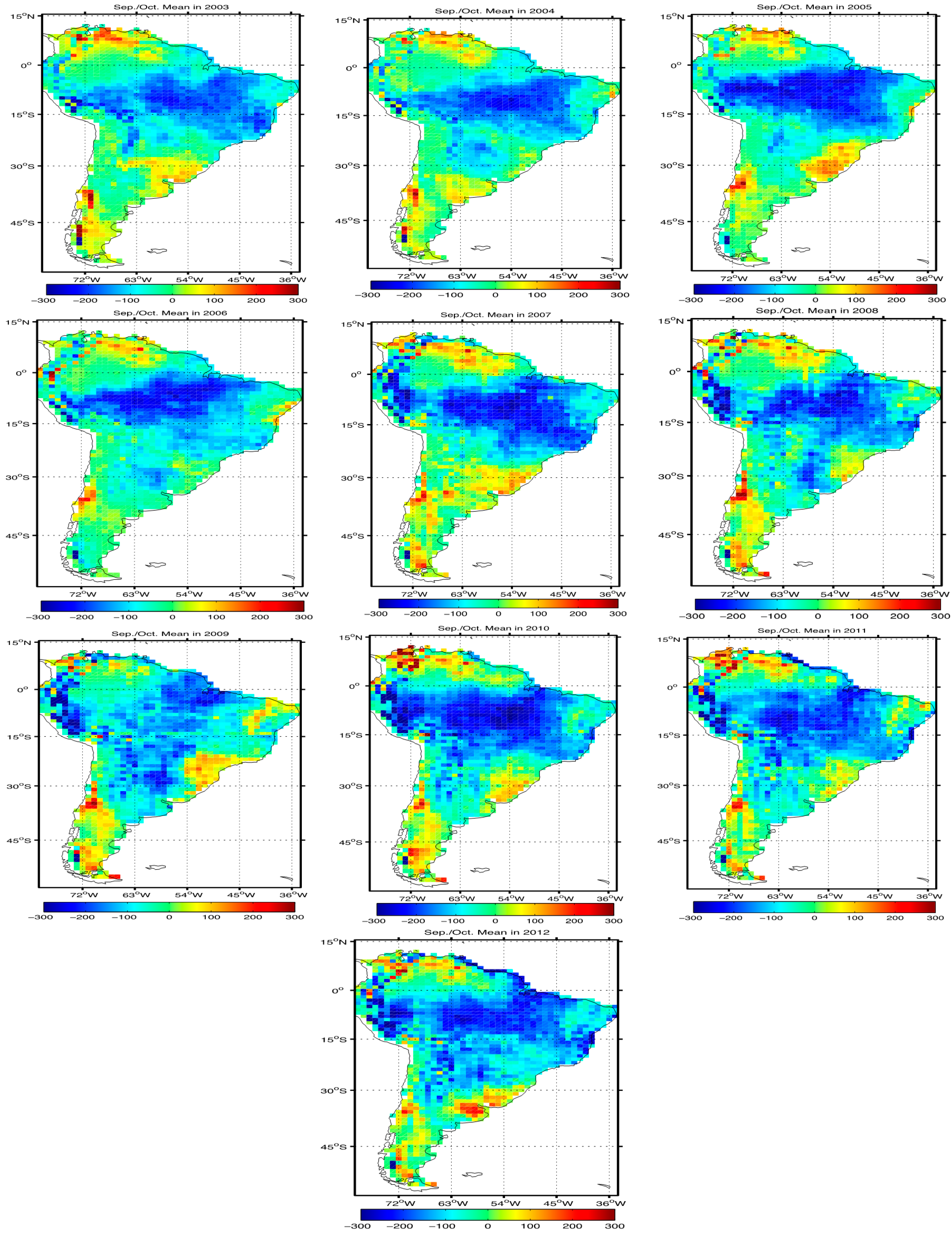
Figure 13.
Logarithm of RMSs of the spherical harmonic coefficients after removing the linear trend, annual and semi-annual cycles from monthly values of each Stoke’s coefficient for GPS+SA and GRACE. Vertical axis is degree n. Horizontal axis represents order m (m < 0 for SINE coefficients, m > 0 for COSINE coefficients). Degree-1 Stoke’s coefficients of GRACE come from [38]. (a) A logarithm of RMSs of GPS+SA Stoke’s coefficients, (b) a logarithm of RMSs of GRACE Stoke’s coefficients.

Figure 14.
Uncertainties of mass errors (in millimeter) estimated from GPS+SA and GRCE after a Gaussian filter with half wavelength at 500 km is applied to both. The used Stoke’s coefficients of GRACE+SA and GRACE are 120-month values in the period 2003–2012. GRACE degree-1 coefficients come from [38]. C(2,0) of GRACE is replaced with C(2,0) of SLR [10]. (a) The GPS+SA mass error with atmosphere and sea. Its global average is 53.99 mm. (b) The GPS+SA mass error without atmosphere and sea. Its global average is 53.36 mm. (c) The GRACE mass error with atmosphere and sea. Its global average is 25.50 mm. (d) The GRACE mass error without atmosphere and sea. Its global average is 22.27 mm.
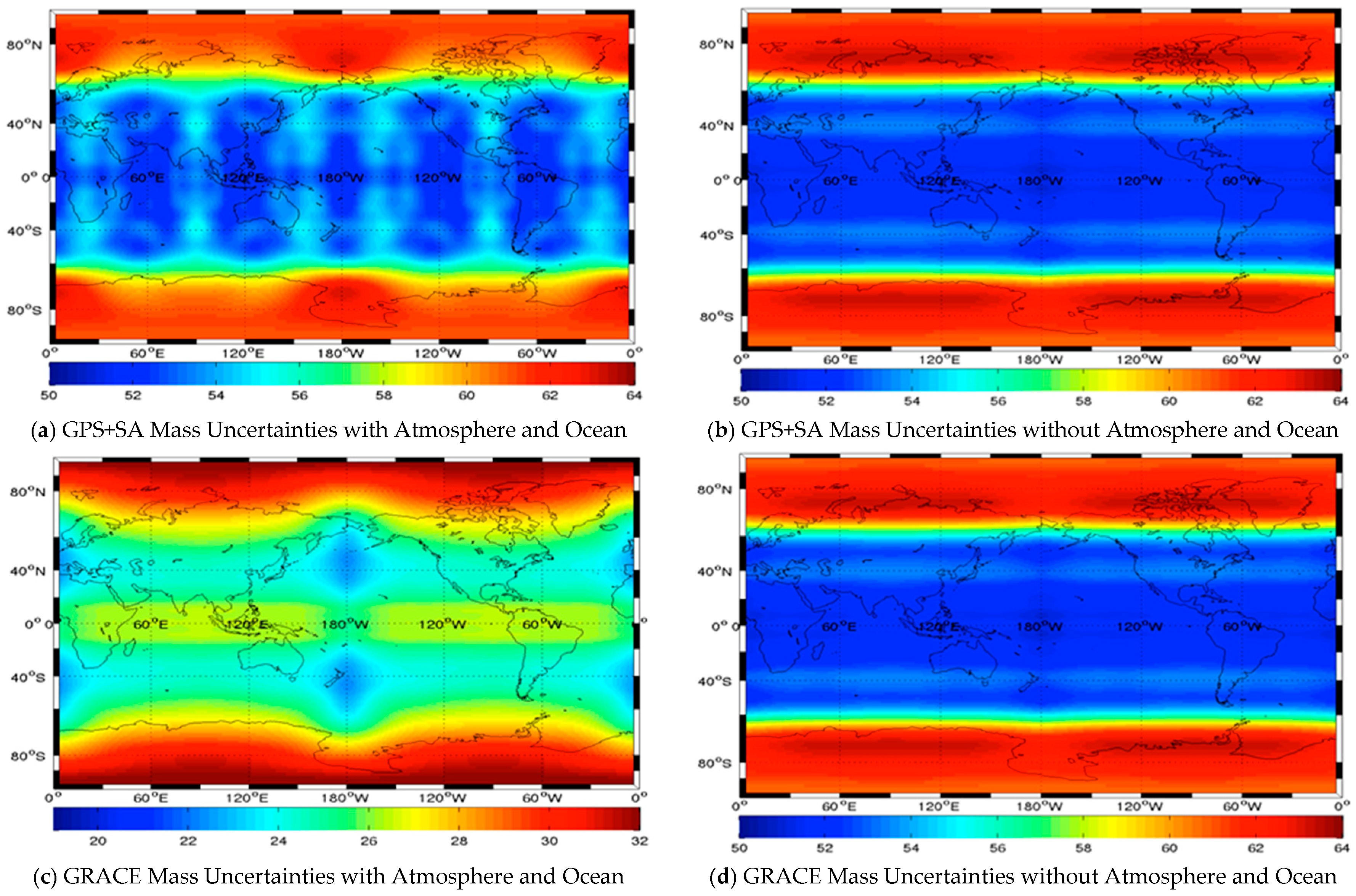
Figure 15.
Contributions of each data set in the joining inversion for Stoke’s coefficients. (a) GPS site displacement contribution to each Stoke’s coefficient; (b) Satellite altimetry (SA) contribution to each Stoke’s coefficient; (c) Contribution of a priori constraint on the amplitudes to each Stoke’s coefficient; (d) GPS, SA and a priori constraint contribution at each degree of Stoke’s coefficients. Positive orders are for the cosine coefficients and negative orders are for the sine coefficients in (a–c).

Table 1.
Annual variations of the geocenter and degree-2 gravity coefficients estimated from GPS+SA, SLR and GRACE. GPS+SA means results combining GPS and SA with the truncation degree at 60. SLR results are from [9,10]. GRACE geocenter is computed by combination of GRACE and OBP [38].
| GPS+SA | SLR | GRACE | |
|---|---|---|---|
| Annual Amplitudes (geocenter unit: mm) | |||
| X | 0.81 ± 0.14 | 4.37 ± 0.29 | 2.26 ± 0.12 |
| Y | 1.79 ± 0.15 | 2.26 ± 0.30 | 2.38 ± 0.09 |
| Z | 2.29 ± 0.19 | 4.54 ± 0.42 | 2.24 ± 0.16 |
| C20 | 1.05 ± 0.14 × 10⁻¹⁰ | 1.39 ± 0.08 × 10⁻¹⁰ | 1.50 ± 0.18 × 10⁻¹⁰ |
| C21 | 0.24 ± 0.09 × 10⁻¹⁰ | 0.23 ± 0.04 × 10⁻¹⁰ | 0.17 ± 0.03 × 10⁻¹⁰ |
| S21 | 0.98 ± 0.08 × 10⁻¹⁰ | 0.86 ± 0.05 × 10⁻¹⁰ | 0.79 ± 0.05 × 10⁻¹⁰ |
| C22 | 0.25 ± 0.08 × 10⁻¹⁰ | 0.13 ± 0.04 × 10⁻¹⁰ | 0.14 ± 0.04 × 10⁻¹⁰ |
| S22 | 0.68 ± 0.09 × 10⁻¹⁰ | 0.62 ± 0.05 × 10⁻¹⁰ | 0.72 ± 0.04 × 10⁻¹⁰ |
| Annual Phases (unit: angular degree) | |||
| X | 83.41 ± 9.80 | 35.12 ± 3.82 | 59.86 ± 3.16 |
| Y | −35.65 ± 4.78 | −23.54 ± 7.44 | −39.70 ± 2.15 |
| Z | 36.25 ± 4.88 | 39.74 ± 5.24 | 69.13 ± 4.26 |
| C20 | 65.44 ± 7.73 | 52.43 ± 3.13 | 38.53 ± 6.85 |
| C21 | −144 ± 22.64 | −1.38 ± 9.69 | −47.60 ± 11.57 |
| S21 | −9.54 ± 4.87 | −14.21 ± 3.47 | −18.19 ± 3.51 |
| C22 | −157.24 ± 17.35 | −120.66 ± 17.88 | −157.91 ± 14.25 |
| S22 | −46.42 ± 7.76 | −49.29 ± 4.28 | −38.01 ± 3.19 |
© 2017 by the authors. Licensee MDPI, Basel, Switzerland. This article is an open access article distributed under the terms and conditions of the Creative Commons Attribution (CC BY) license (http://creativecommons.org/licenses/by/4.0/).
Share and Cite
MDPI and ACS Style
Zhang, X.; Jin, S.; Lu, X. Global Surface Mass Variations from Continuous GPS Observations and Satellite Altimetry Data. Remote Sens. 2017, 9, 1000. https://doi.org/10.3390/rs9101000
AMA Style
Zhang X, Jin S, Lu X. Global Surface Mass Variations from Continuous GPS Observations and Satellite Altimetry Data. Remote Sensing. 2017; 9(10):1000. https://doi.org/10.3390/rs9101000
Chicago/Turabian StyleZhang, Xinggang, Shuanggen Jin, and Xiaochun Lu. 2017. "Global Surface Mass Variations from Continuous GPS Observations and Satellite Altimetry Data" Remote Sensing 9, no. 10: 1000. https://doi.org/10.3390/rs9101000
Note that from the first issue of 2016, this journal uses article numbers instead of page numbers. See further details here.