A Methodology to Detect and Update Active Deformation Areas Based on Sentinel-1 SAR Images

Abstract

This work is focused on deformation activity mapping and monitoring using Sentinel-1 (S-1) data and the DInSAR (Differential Interferometric Synthetic Aperture Radar) technique. The main goal is to present a procedure to periodically update and assess the geohazard activity (volcanic activity, landslides and ground-subsidence) of a given area by exploiting the wide area coverage and the high coherence and temporal sampling (revisit time up to six days) provided by the S-1 satellites. The main products of the procedure are two updatable maps: the deformation activity map and the active deformation areas map. These maps present two different levels of information aimed at different levels of geohazard risk management, from a very simplified level of information to the classical deformation map based on SAR interferometry. The methodology has been successfully applied to La Gomera, Tenerife and Gran Canaria Islands (Canary Island archipelago). The main obtained results are discussed.

1. Introduction

This paper is focused on geohazard activity mapping and monitoring using Sentinel-1 (S-1) data and the DInSAR (Differential Interferometric Synthetic Aperture Radar) technique. In the last 25 years, the mapping and monitoring of geohazard phenomena have received an important contribution from the DInSAR technique. This approach was firstly proposed in 1989, using data from the L-band Seasat sensor [1]. Since then, the technique has experienced a continuous growth mainly related to two main components. The first one is the important research and development effort made in this period, which has generated a wide number of data processing and analysis tools and methods. They include the classical single-interferogram DInSAR methods (e.g., see [2,3,4]), the DInSAR stacking techniques [5] and several implementations of the so-called Persistent Scatterer Interferometry (PSI) and Small Baseline Subsets (SBAS) methods [6,7,8,9,10]. A review of all these advanced methods, which are sometimes referred to as Advanced DInSAR (A-DInSAR) or Time Series Radar Interferometry (TSInSAR), is provided in [11]. In the last years, the number of DInSAR users has increased thanks to the availability of free platforms and software, such as Grid Processing on Demand (G-POD) and Sentinel Application Platform (SNAP), provided by ESA, which have widened the range of potential users [12,13].

The second component is satellite data availability, which has increased in terms of number of satellites with different spatial and temporal resolutions. Most of the DInSAR and PSI developments have been based on C-band data acquired by the sensors on-board the satellites ERS-1/2, Envisat and Radarsat. The available imagery collected by these satellites cover long periods of time (starting from 1992), a key aspect to guarantee a long-term deformation monitoring and to make historical studies [14]. DInSAR and PSI have experienced a major step forward since 2007, with the advent of very high-resolution X-band data [15] of TerraSAR-X and COSMO-SkyMed. This includes the capability to generate a dense sampling of Persistent Scatterers (PS), a high sensitivity to small displacements and a remarkable quality improvement of the time series with respect to the C-band [16,17]. Those improvements have had an important impact on the geohazard applications, improving the analysis at different scales and allowing the combination of the results from different satellites [18,19,20,21,22,23,24]. A review over the available satellite SAR sensors and their potentialities for landslide application can be found in [25,26]. A significant further improvement is given by the new C-band sensor on-board the S-1A and B satellites, launched on 2014 and 2016, respectively [27]. S-1 has improved the data acquisition throughout and, compared to previous sensors, has increased considerably the DInSAR and PSI deformation monitoring potential [4,28] allowing to make long-term geohazard monitoring planes over regional areas [29].

This work is aimed at exploiting the wide area coverage and the high coherence [4] and temporal sampling (revisit time up to six days) provided by the S-1 satellites to generate and periodically update regional-scale deformation activity maps for the geohazard management. The proposed methodology has been developed in the framework of the ongoing European ECHO (European Civil Protection and Humanitarian Aid Operations) project “Safety—Sentinel for geohazards regional monitoring and forecasting”, which aims at providing Civil Protection Authorities (CPA) with the capability of periodically evaluate and assess, at regional scale, the potential impact of geohazards (volcanic activity, landslides and subsidence) on urban areas.

The interpretation of the DInSAR derived maps (e.g., velocity maps) can be complex, mostly for users who are not familiar with radar data [30,31]. This is more evident working at regional scale, where the high number of PSs can difficult the analysis and in some cases misinterpret the real scenario. Several authors have shown different approaches to address this issue [25,32]. This work presents a procedure to generate clear products that can be easily exploited by the authorities involved in the geohazard and risk management chain. The main output is the so-called Active Deformation Areas (ADA) map. It is derived from the DInSAR Deformation Activity Map (DAM) by discriminating the more reliable deforming areas. A further step, which is the integration of the products of the methodology (DAM and ADA maps) in the Civil Protection risk management activities, is described in [33].

The procedure is illustrated through its application over the Canary Islands, a Spanish volcanic archipelago located in the Atlantic Ocean, northwest of Africa, which is one of the test sites of the Safety project. Canary Islands present different types of geohazards, including landslides, earthquakes and volcanic activity.

The paper starts with the description of the procedure (Section 2), then the results of the active deformation maps obtained over the Canary Islands test site are described (Section 3). This is followed by the discussion of the results by emphasizing the main advantages and main challenges of the proposed approach (Section 4). Finally, the conclusions of the work are drawn (Section 5).

2. Methodology

In this section, the procedure to derive the DAM and the ADA maps is described. The proposed procedure can be applied to the data acquired by any satellite SAR sensor. However, it provides the best performances with the S-1 characteristics.

The general scheme of the procedure, shown as a flowchart in Figure 1, is divided in two main blocks (Figure 1):

• Raw Deformation Map (RDM) generation: This includes all the PSI processing steps to estimate the annual linear velocities and the time series of deformation (TS). The RDM is an intermediate product that is not delivered to the final users.
• Deformation Activity Map (DAM) generation and Active Deformation Areas (ADA) extraction: In this block, the two final products of the procedure are generated. It includes a filtering of the RDM and all the steps to generate the ADA map. These two products are easily readable and thus exploitable by the risk management decision makers.

All the deformation values included in the output maps are estimated along the satellite Line of Sight (LOS) direction. The procedure is designed to be periodically processed to have a continuous update of the products and thus a continuous input of regional-scale deformation maps for the authorities to detect potential hazards or to decide more focused analysis in critical areas.

2.1. Raw Deformation Map Generation

The main goal of this block is to derive the deformation scenario of an area of interest from the SAR data. The output is a deformation map that consists in a set of selected points with both the information of the estimated LOS velocity and the accumulated displacement at every satellite acquisition. The main input is a set of SAR images acquired at different times. Several Persistent Scatterer Interferometry (PSI) techniques have been developed in the last decade. The main common steps to generate a deformation map are: the interferogram network generation, the selection of points, the phase unwrapping, the Atmospheric Phase Screen (APS) estimation and removal and the estimation of the velocities and/or deformation time series (TS). The choice between the different techniques depends on many factors like the radar sensor characteristics, the target of the study or the characteristics of the test site (geology, land use, topography, etc.). In particular, for this research, the maps have been generated using an approach of the Persistent Scatterer Interferometry chain of the Geomatics (PSIG) Division of CTTC (PSIG) described in [32]. The main steps of the processing are briefly described in the following lines (Figure 2):

• Interferogram network generation: This step consists of the generation of the interferogram network. S-1 uses a sophisticated data acquisition procedure, the TOPS (Terrain Observation by Progressive Scan) imaging mode [34], which is key to achieve the wide area coverage. The drawback is that, compared to other sensors, the S-1 data require extra processing. The key step is the image co-registration, which needs to be very accurate [35].
  Since a fundamental aspect of the PSIG chain is the redundancy of the network of interferograms and images, all the possible interferogram pairs are generated. The selection of the interferogram network is done by statistically evaluating the coherence of the study area. This analysis provides key inputs for the network like the maximum temporal baseline to be used as well as the presence of periods characterized by low coherence (e.g., snow periods in mountain areas). As example, in the Canary Islands test site, the selected maximum temporal baseline was 156 days.
• Point Selection: Even if a single S-1 frame contains millions of pixels, only a small portion of them is exploitable for deformation purposes. There are different statistical criteria used to discriminate the noisier pixels from those with low level of noise [11]. However, the use of very restrictive thresholds can result in a critical loss of spatial coverage. The general purpose of this step is to find a good compromise between the quality of the selected points (little affected by noise) and a good spatial coverage. Hence, for each case, different criteria are evaluated in order to find the best trade-off. For example, in the Canary Islands test site, the selection of points was based on the Dispersion of Amplitude (DA) [6]. Only points with a DA value lower than 0.5 have been selected.
• 2+1D phase unwrapping: This is a two-step spatial-temporal phase unwrapping [32]. The approach starts with a spatial phase unwrapping (2D) performed over the selected set of points and for each interferogram of the network. Then, in a second phase, a phase unwrapping consistency check (1D) is performed. This check is done point wise, exploiting the temporal component of the SAR images stack. It is based on an iterative least squares method (LS) and the analysis of the LS residuals at each iteration. For each pixel, the main outputs are: (i) the temporal evolution of the phases (TEP) with respect to a reference image; and (ii) some statistical parameters used to assess the quality of the LS inputs.
• APS (Atmospheric Phase Screen) estimation and removal: The APS is estimated using spatial-temporal filters [36]. The main input is the TEP estimated in the previous step. The estimated APS is removed from the TEP. The remaining phases are then transformed into deformations, obtaining the final deformation time series (TS).
• Deformation velocity estimation: This is the last step of the deformation map generation block. It consists of an estimation of the deformation velocity from the obtained time series. The used method is a robust regression line estimation.

The final output of this block is a raw deformation map (RDM) including, for each point, the deformation velocity and the accumulated deformation at each acquisition time (TS). The estimated deformations are in the satellite LOS direction.

It is worth noting that the described approach can slightly change depending on the site. A frequent variation is to perform the deformation velocity estimation before the 2+1D phase unwrapping. The deformation velocity is estimated over the wrapped phases and then removed from them before the phase unwrapping [5]. This is done to ease the 2D phase unwrapping step in areas strongly affected by deformation.

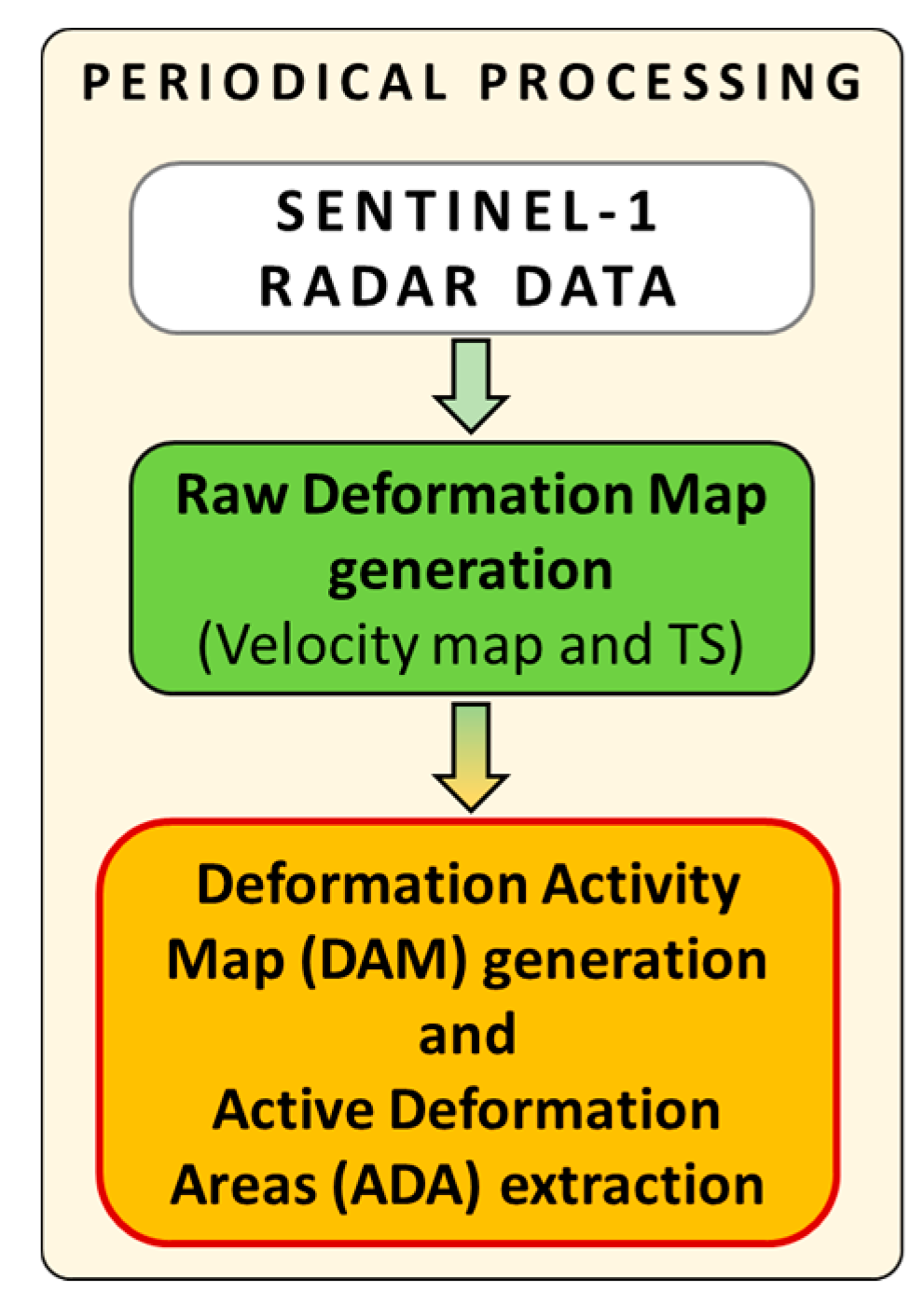
2.2. Deformation Activity Map and Active Deformation Areas Extraction

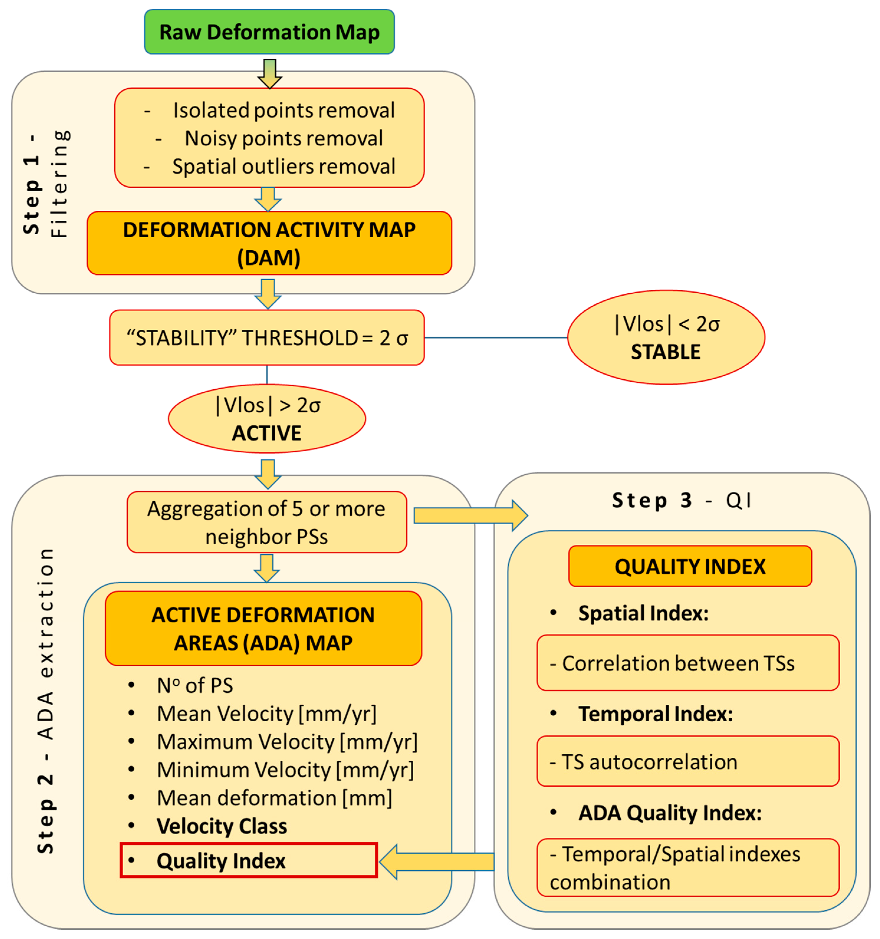
This block is aimed at obtaining both the final Deformation Activity Map (DAM), which is the filtered version of the raw deformation map (RDM), and the Active Deformation Areas (ADA) map, which is the main product of the procedure. The main goal is to identify and monitor, over wide areas, the most critical deformations to provide the Civil Protection authorities with the capacity to perform prevention and mitigation actions. Therefore, the three main aspects that have to characterize the final maps are: (i) the readability; (ii) the reliability; and (iii) the regional-to-local scale. The main constraining factors to achieve these goals are the spatio-temporal noise of the deformation map and the high number of PSs which in some cases can lead to wrong interpretations.

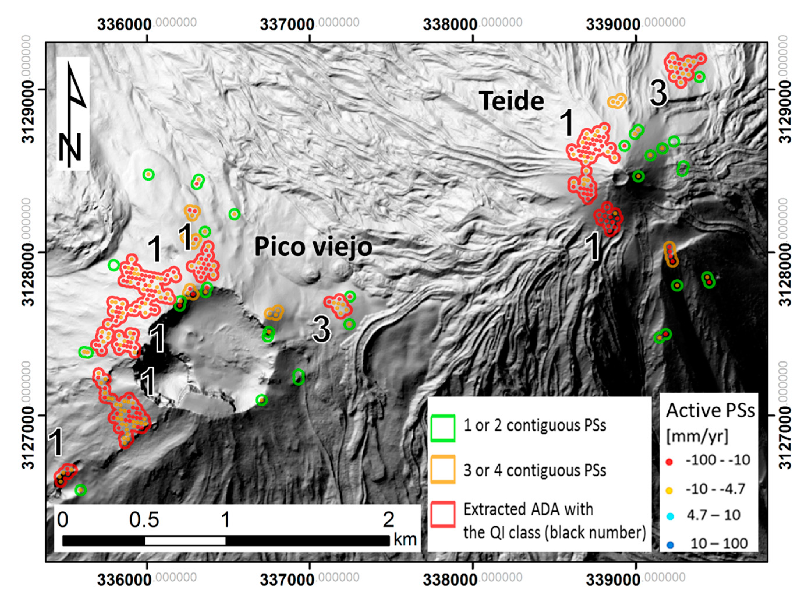
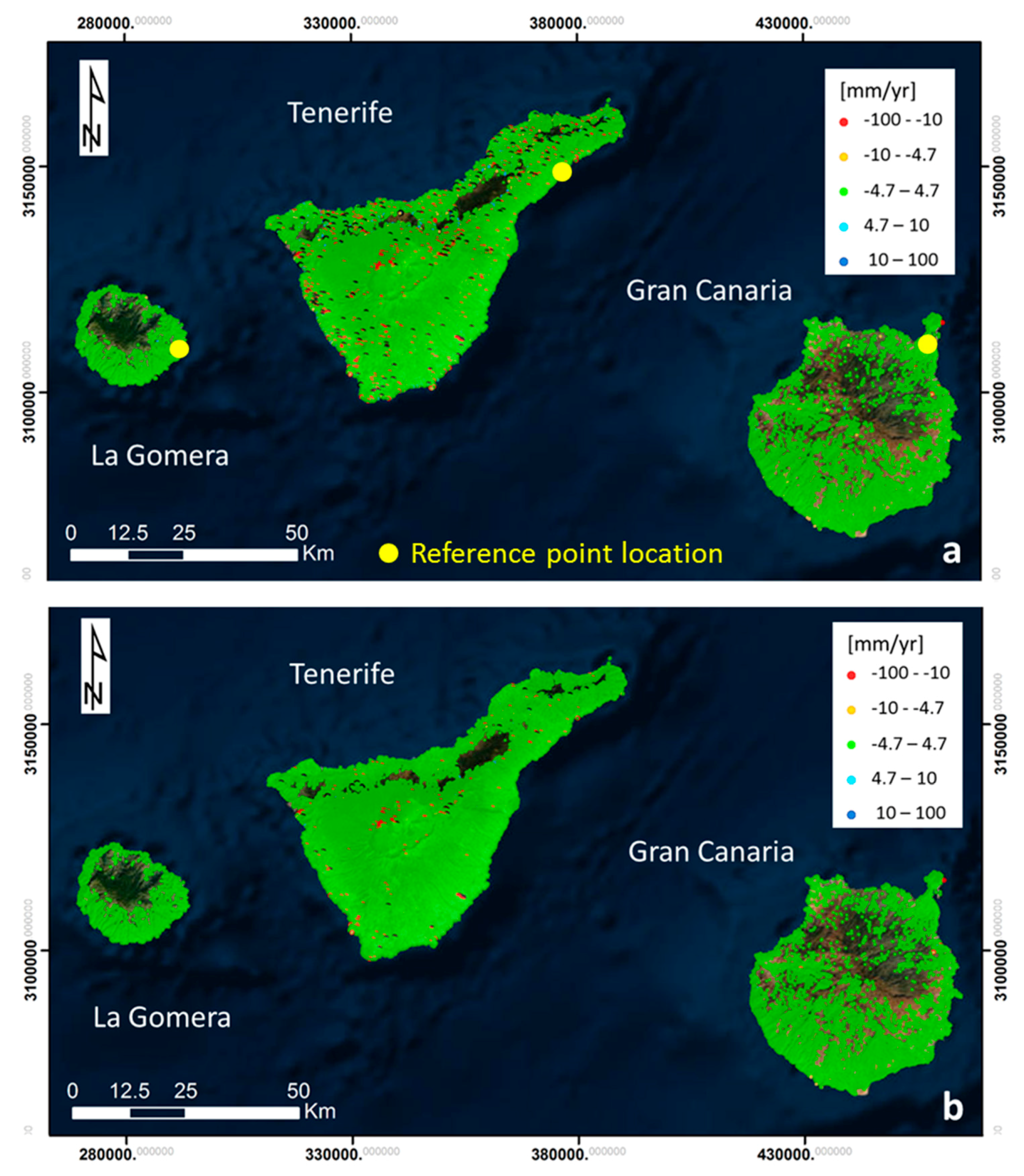
A key parameter of this block is the assessment of the general noise level (sensitivity) of the RDM. In this research, the sensitivity has been evaluated using the standard deviation (σ_map) of the RDM velocity values. A stability threshold of 2σ_map is set to distinguish the active points, those where we measure movements, from those we do not. A point is considered moving if |v| > 2σ_map, where |v| is the absolute velocity value of the point. It is worth to underline that the points classified as “stable” can be truly stable as well as instable points, with a not detectable movement. To simplify the readability, we call “stable” all the points with the absolute LOS velocity below the stability threshold. As example, in the Canary Island test site, the stability threshold has been set as ±4.7 mm/year.

This block can be summarized in three main steps (Figure 3): (i) filtering of the RDM; (ii) automatic extraction of the more reliable and relevant active areas (ADA); and (iii) Quality Index (QI) attribution to each ADA.

(i) Filtering of the raw deformation map

This action aims to filter the RDM obtained in block 1. The final point selection has been based on two different criteria: (i) the standard deviation of the 2+1D phase unwrapping residues (σ_res); and (ii) a spatial criterion based on the variability of a point with respect its neighbors. The first one is used to remove points susceptible to be affected by phase unwrapping errors. The used threshold for the σ_res is 2.4 rad (approximately 1 cm). We have selected this relatively high threshold in order to keep the maximum number of measurements. Regarding the spatial criterion, it is used to clean sparse measurements (isolated points) and points with strong discrepancy with respect its neighbors (outliers). The filtering is window based. The used window has a radius of 2 times the data resolution (e.g., around 80 m in Canary Island).

The filtering criteria are: (i) eliminate points without neighbors inside the window; and (ii) eliminate moving points without more than one moving neighbors inside the window. It is worth noting that the eliminated points can be real moving points related to a geohazard, like for example a landslide. However, an isolated point can be related to several factors including noise. In this context, we accept to lose information about few phenomena in order to highly reduce the general level of noise and simplify the readability of the map.

(ii) Automatic extraction of the more reliable and relevant active areas (ADA)

The aim of the ADA map generation is to perform a rapid identification of the most reliable active deformation areas. The final map has to represent a clear input to be validated and integrated with other data (e.g., geohazard inventories, ground truth information, etc.) in order to determine the nature of the deformation and thus to generate the Geohazard Activity Map.

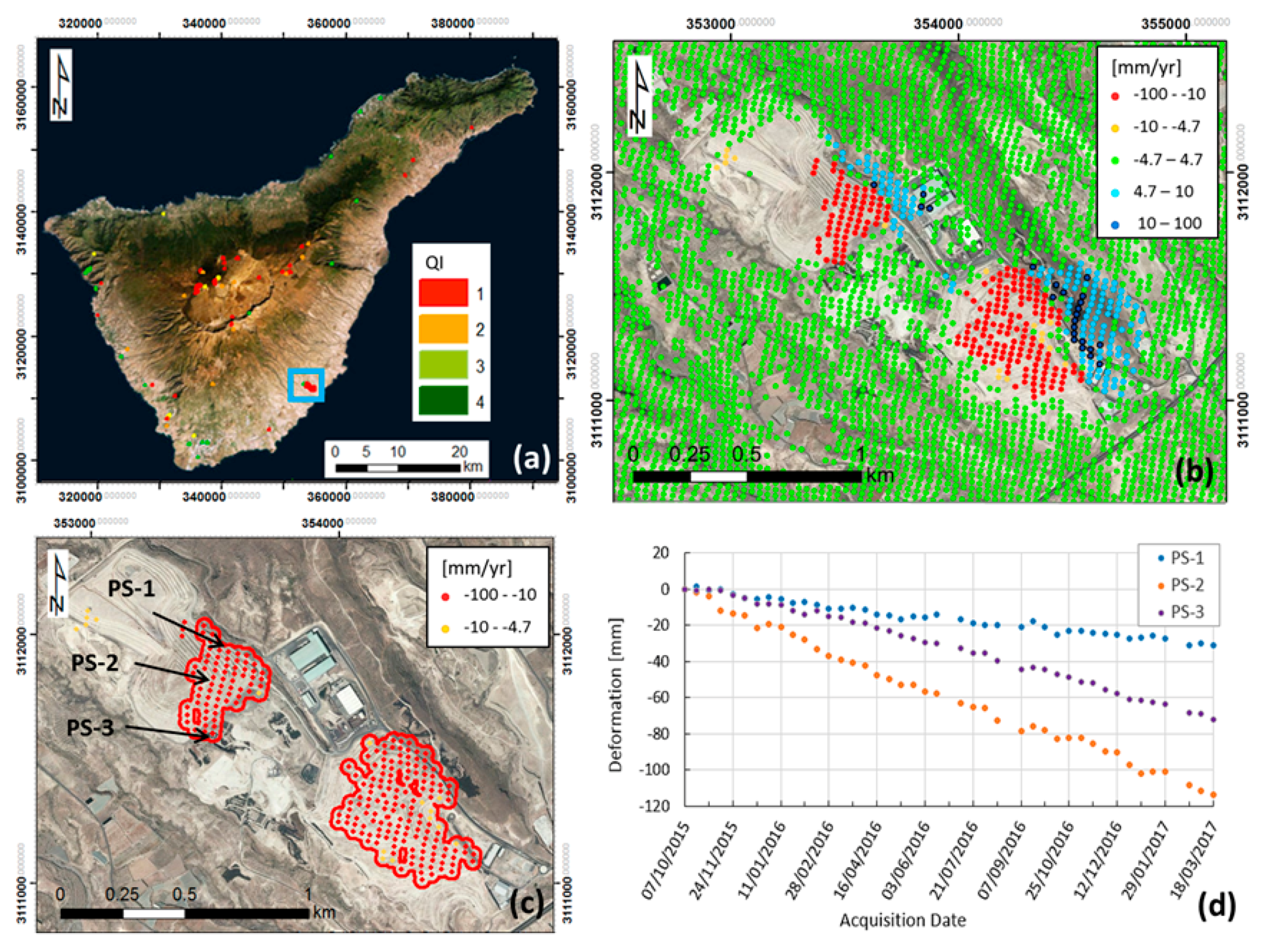
The ADA map has been by using an evolution of the approaches proposed by [37,38,39,40]. The main input is the filtered deformation velocity map obtained in Step (i). Only the moving points (with |v| > 2σ_map) are selected. Then, from this subset of points (PSm), groups of at least five neighbor PSs, sharing their influence area, are aggregated in polygons representing the Active Deformation Areas (ADA). To define the influence area of every PS we consider the approximated footprint of the PSs. For example, in Canary Island test site, the PS area is of 28 m by 40 m. Then we calculate the radius of the circle inscribing the PS area (40 m by 40 m in the Canary Island Site) and we multiply it by a factor of 1.3 to ensure that neighboring pixels are selected. If the grouped PSs are less than five, they are considered to represent a non-significant deformation for a regional scale map.

Finally, for each ADA, the following parameters are estimated:

-

Number of aggregated active points (APs).

-

Mean, maximum and minimum values of the APs velocities.

-

Mean value of the APs accumulated deformations. To avoid strong influence of atmospheric or digital elevation model error effects, we estimate the final accumulated deformation as the average of the accumulated values of the last four acquisition times of all the APs of the ADA.

-

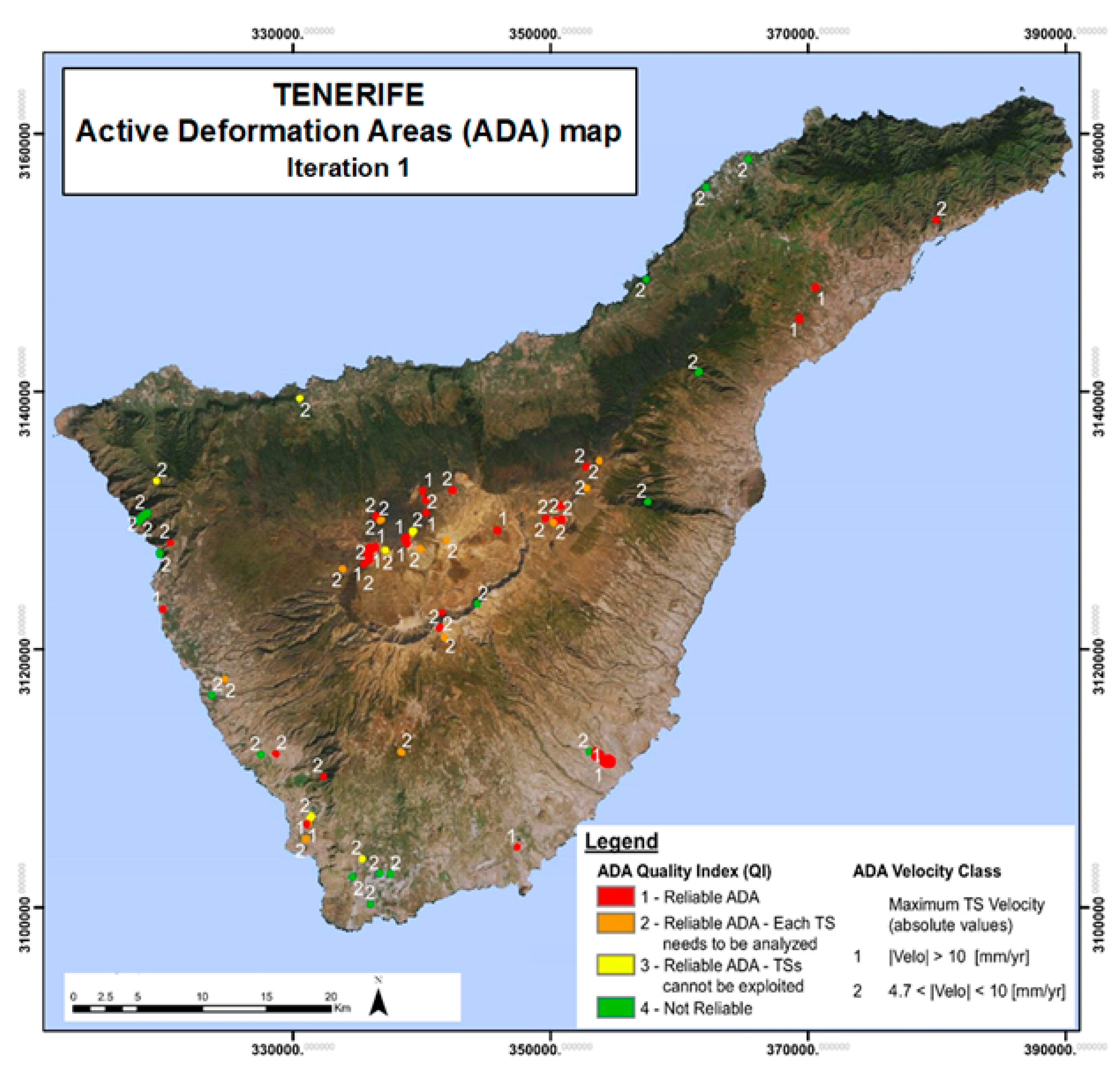
Velocity class, which is a classification of the ADA as a function of its maximum velocity (v_m). The class is 1 if |v_m| > 1 cm/year or 0 if 2σ_map < |v_m| < 1 cm/year.

-

Quality Indexes, which are explained in the following lines.

(iii) Quality index attribution to each ADA

Although the ADA map is based on filtered data, the automation of the process needs a final quality assessment for each single ADA. The noise level of the TSs and thus the robustness of the deformation estimations vary significantly pointwise. This step describes an implemented Quality Index (QI) that provides an estimation of the noise level of the ADA. This QI is a key parameter to properly interpret the ADA map.

The QI is based on the evaluation of two parameters for each ADA: the noise of each AP time series is evaluated and the spatial homogeneity of the estimated deformations in time is considered (i.e., consistency between AP time series). Hence, each ADA is characterized by a temporal noise index (TNI) and a spatial noise index (SNI) that are used to derive the final QI.

• Temporal Noise Index (TNI)

To attribute the TNI, for each APs the first order autocorrelation (ρ_t,t−1) of its TS is evaluated. The first order autocorrelation allows evaluating the temporal noise degree for both linear and nonlinear deformation trends. The autocorrelation coefficient ranges from 0 to 1, where 0 means the prevalence of noise over the deformation trend. The temporal index (TNI) is a four-class classification of the ADA based on the median value (Med(ρ)) between the TS autocorrelation coefficients, it varies from 1 to 4, where 1 corresponds to a high Med(ρ) and 4 to a very low Med(ρ).

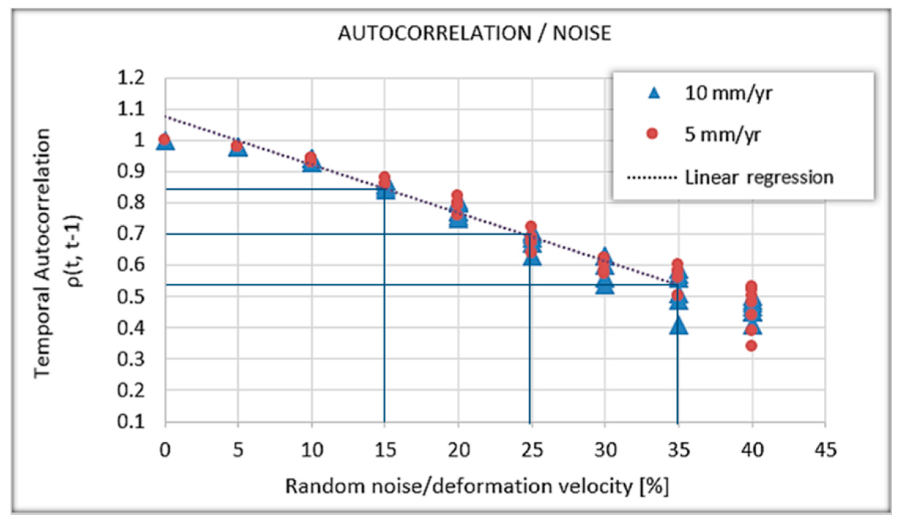
To find a relationship between the autocorrelation coefficient and the noise level, a simulation was performed on a set of 20 TSs characterized by a linear trend (b) and random noise (ϵ):

Y = bx + ϵ

where b = velocity in (mm/day), x = 0, 12, 24, 36,…, 468 (days) is the 12 days spaced time series. The random noise was characterized by a normal distribution. For each velocity, we tested different levels of noise by setting the standard deviation of the simulated random noise. Since the autocorrelation also depends on the number of sampling (i.e., on the length of the TS and the revisit time), our simulation was calculated over 468-day time series (almost one year and half) with temporal steps of 12 days. This period corresponds to the temporal window used to generate the deformation maps in our test site (Canary Islands). Figure 4 shows the results of the two simulations performed with the velocities of 5 and 10 mm/year. The plotted values represent the median value of the set of TSs autocorrelation coefficients calculated for each tested noise level. By expressing the noise level in terms of percentage of the velocities, the relationship can be approximated by the linear regression of the whole data resulted by the simulation.

It is worth mentioning that this is a simplified model, helpful to evaluate the physical meaning of the thresholds. Note that, for equal noise level, the autocorrelation coefficient changes with temporal sampling. Therefore, the thresholds can change, depending on the study case, if both the Sentinel-1A and Sentinel-1B images are used (six-day revisit time).

The ρ_t,t−1 values of 0.53, 0.70 and 0.84, respectively, corresponding to the 35%, 25% and 15% of noise with respect to the velocities (Figure 4 and

Table 1. Final classification of TNI.

Med(ρ)	Noise-Velocity Ratio (%)	Class
<0.53	>35	4
0.53–0.70	35–25	3
0.70–0.84	25–15	2
>0.84	<15	1

), were chosen as thresholds for the four classes of TNI.

• Spatial Noise Index (SNI)

The aim of the SNI estimation is to evaluate the spatial consistency of the detected ADA, i.e., to quantify how the PSs composing an ADA evolve with a similar trend. We assume that all the TSs of the same ADA belong to the same deformation phenomena. Thus, we expect different magnitude of the detected movements, but a spatial correlation between their temporal evolutions. With this aim, for each ADA the correlation coefficient between all the possible pairs of TSs are calculated (CORR(Xi,Yj), where i,j represents all the possible pair combinations of the APs and Xi and Yj are their respective TSs. The spatial index (SNI) is a four-class classification of the ADA based on the median value (Med(CORR)) of all the ADA’s TSs pairs correlation values. It varies from 1 to 4 where 1 corresponds to a high Med(CORR) and 4 to a very low Med(CORR). The classification thresholds (

Table 2. Final classification of the Spatial Noise Index (SNI).

Med(ρ)	Cumulative Frequency (%)	Class
<0.53	<2	4
0.53–0.7	2–25 (1st quantile)	3
0.7–0.84	25–75 (2nd and 3rd quantiles)	2
>0.84	>75 (4th quantile)	1

) have been set on the statistical distribution of the results, specifically the values corresponding to the quartiles that have been chosen.

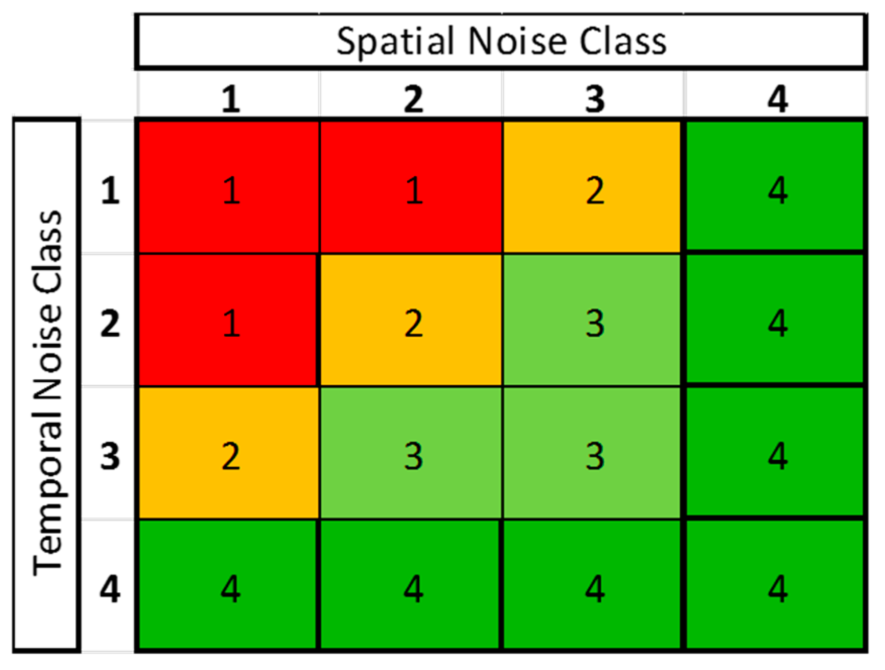
• ADA Quality Index (QI)

The global QI is derived from the combination of both the TNI and the SNI, and measures the degree of reliability of each detected ADA. The numerical classes (QI) assigned to each TNI-SNI combination are represented by the matrix shown in Figure 5. The QI ranges from Class 4, which is the noisiest one, to Class 1, which represents the ADA characterized by very high quality time series (TS). More in detail: Class 4 represents a not reliable ADA; Class 3 means reliable ADA but TS that cannot be exploited; Class 2 means reliable ADA, but a further analysis of the TS is recommended; and Class 1 means reliable ADA and TS.

3. Canary Island Results

In this section, the results of the above application of the procedure over the Canary Islands and some related technical aspects are discussed and presented.

The explained procedure has been applied to three islands: La Gomera, Tenerife and Gran Canaria (Spain). The test-site, covering a total land surface of around 4000 km², allows testing the regional scale potentialities of the procedure.

3.1. Dataset Description

The three islands are covered by a single Sentinel-1 frame. In particular, three swaths and 18 bursts have been processed. In

Table 3. Main characteristics of the processed data.

Satellite	Sentinel-1A
Acquisition mode	Wide Swath
Period	November 2014–March 2017
Minimum revisit period (days)	12
Wavelength (λ) (cm)	5.55
Polarization	VV
Full resolution (azimuth/range) (m)	14/4
Multi-look 1 × 5 resolution (azimuth/range) (m)	14/20
Multi-look 2 × 10 resolution (azimuth/range) (m)	28/40
Orbit	Descending
Incidence angle of the area of interest	36.47°–41.85°

, the main characteristics of the used dataset are described. The used image dataset consists of 64 Sentinel-1 Wide Swath images covering around a two years and a half period, with the first acquisition time in November 2014 and last acquisition time in March 2017. In this study only images from Sentinel-1A satellite have been used, thus the minimum temporal sampling is 12 days, while the maximum temporal sampling, which is defined by the images availability, is 48 days.

Table 4. List of the acquisition dates of the dataset. The intersection between both periods is in bold.

Image	Date	Image	Date	Image	Date	Image	Date
1	5 November 2014	18	8 August 2015	35	28 February 2016	52	13 October 2016
2	17 November 2014	19	20 August 2015	36	11 March 2016	53	25 October 2016
3	29 November 2014	20	1 September 2015	37	23 March 2016	54	6 November 2016
4	11 December 2014	21	13 September 2015	38	4 April 2016	55	18 November 2016
5	23 December 2014	22	25 September 2015	39	16 April 2016	56	30 November 2016
6	4 January 2015	23	7 October 2015	40	28 April 2016	57	12 December 2016
7	16 January 2015	24	19 October 2015	41	10 May 2016	58	24 December 2016
8	28 January 2015	25	31 October 2015	42	22 May 2016	59	5 January 2017
9	9 February 2015	26	12 November 2015	43	3 June 2016	60	17 January 2017
10	21 February 2015	27	24 November 2015	44	15 June 2016	61	29 January 2017
11	5 March 2015	28	6 December 2015	45	9 July 2016	62	22 February 2017
12	17 March 2015	29	18 December 2015	46	21 July 2016	63	6 March 2017
13	29 March 2015	30	30 December 2015	47	2 August 2016	64	18 March 2017
14	9 June 2015	31	11 January 2016	48	14 August 2016
15	3 July 2015	32	23 January 2016	49	7 September 2016
16	15 July 2015	33	4 February 2016	50	19 September 2016
17	27 July 2015	34	16 February 2016	51	1 October 2016

shows the list of all the acquisition times of the processed images.

As explained in the introduction, the aim of the procedure is to generate and periodically update deformation activity maps. With this aim, the dataset has been divided in two parts and processed separately to produce and compare two versions of the ADA map: version V1 and the temporally-updated version V2. The temporal windows covered by the two processing iterations and the number of the processed images are resumed in Table 4: for the first iteration, 51 images covering a period of around two years have been processed; and, for the second iteration, 42 images covering a period of one and a half years have been processed, the overlapping period between the two iterations is one-year long. Furthermore, considering the specific radiometric characteristics of the test-site, using temporal windows of one and a half years, to be processed each six months (i.e., with an overlapping period of six months) is the ideal way of generating and updating the maps.

The SRTM Digital Elevation Model provided by NASA has been used to process the interferometric products [41].

3.2. Deformation Activity Maps

To derive the deformation maps, we have generated a network of 398 interferograms in the first iteration and 481 interferograms in the second iteration. The maximum temporal baseline used is 156 days. This threshold has been derived by statistical analysis of the coherence with respect to the temporal baseline. The reference points used for the processing are located in the historical centres of the three capitals of the islands (Figure 6a): San Sebastián de La Gomera; Santa Cruz de Tenerife; Las Palmas de Gran Canaria.

Due to the geologic and land cover settings, mainly of sparse vegetation and rocky surfaces, Canary Islands show a good radar response in terms of coherence. This characteristic results in a deformation map characterized by both a high coverage of points and a low spatio/temporal noise. Figure 6 shows the high density of points of the velocity map: only the few zones covered by forest show absence of points (northern humid flanks of the islands). The noise level of the map (i.e., the sensitivity) was estimated as two times the standard deviation of the velocity of all the measured points and is equal to 4.7 mm/year for both iterations. This value (see Section 2) also represents the stability threshold, i.e., the value that separates the moving points from the points with no-detected movement (stable points).

As explained in Section 2, three filters have been applied to the raw deformation map in order to reduce the spatio-temporal noise and thus to improve the readability and the reliability of the map measurements. Figure 6 shows the velocity map resulted from the first iteration before and after the spatial filtering. After the filtering, the number of measured points of the Deformation Activity Map (DAM) is 1,060,750 for the first iteration and 1,036,328 for the second iteration. The total number of points identified as non-stable is 2358 in the first iteration and 1859 in the second one, which represents less than 1% of the total number of measured points.

3.3. Active Deformation Areas (ADA) Map

To extract the ADA from the DAM, the methodology shown in Figure 3 and explained in Section 2 has been applied. Figure 7 shows an example of ADA extraction over the Pico Viejo-Teide area, in the heart of Tenerife Island: only the active PSs are visualized, the red polygons are examples of extracted ADA (five or more active contiguous PSs), the green polygons highlight the spatial outliers PSs (one or two active isolated PSs), which are not included in the final DAM, while the orange polygons are active PSs that are not extracted as ADA (three or four contiguous PSs) but are included in the DAM for a local scale analysis. Figure 8 shows an example of two extracted ADA, located southeast of Tenerife (Figure 8a), which are both subsidence phenomena related to the activities of a waste dump. Figure 8b presents the DAM of the waste deposit area. There are four areas affected by movements, two with subsidence (red) and two with uplift (blue), both related to the waste dump activities.

Figure 8c shows the two ADA affected with subsidence in Figure 8b. Figure 8d shows the time series of three PSs located, as indicated in Figure 8c, in one of the two ADA. The area is classified with both the SNI and the TNI equal to 1, which means that the ADA is characterized by the highest spatial and temporal quality. It is interesting to note that the SNI method evaluates the spatial noise in terms of spatial homogeneity of the ADA temporal evolution and is not affected by the spatial variation of the deformation magnitude. In this case, for example, the ADA presents very different velocities, following the subsidence spatial distribution, with the higher deformation rate in the centre of area (Figure 8c,d, PS-2) and the lower ones in the peripheral zones (PS-1 and PS-3). This subsidence area is active in both iterations, without a significant change in the mean velocity (less than the sensitivity of the map): −41.4 mm/year in the first iteration and −40.4 mm/year in the second iteration.

For each ADA, the information resumed in

Table 5. The attributes associated to each ADA.

Field	Description	Units
Join Count	Number of unstable points grouped in the hotspot	-
Fi	WGS84 Geographic Latitude (average of the grouped PSs)	°
Lambda	WGS84 Geographic Longitude (average of the grouped PSs)	°
E	WGS84 UTM zone 32N—East (average of the grouped PSs)	m
N	WGS84 UTM zone 32N—North (average of the grouped PSs)	m
H	SRTM Height (average of the grouped PSs)	m
Acc. Defo.	Accumulated deformation (average of the grouped PSs)	mm
Velocity mean	Mean velocity of the hotspot (average of the grouped PSs)	mm/year
Velo max	Maximum velocity of the PSs grouped in the hotspot	mm/year
Velo min	Minimum velocity of the PSs grouped in the hotspot	mm/year
QI	Quality index of the ADA	-
Class	Classification of the hotspots based on the Velo max.	-

is collected, forming the attribute table of the corresponding polygonal shapefile. This include the velocity class, which allows enhancing the visualization of the most critical ADA in terms of magnitude of deformation, and the QI class, which is a fundamental information for the interpretation of the map. An example of ADA map visualization of both the QI and the velocity class information is presented in Figure 9. In the first iteration, 72 ADA has been extracted: 69 are localized on Tenerife Island and the other three on Gran Canaria. In the second iteration, 120 ADA have been detected: 112 are on Tenerife, seven on Gran Canaria and one on Gomera. In total, 68% of the ADA detected in the first iteration (V1) fall in the QI classes 1 and 2, while, in the second iteration (V2), the percentage of 1 and 2 QI drops to 43% (see the Total columns of

Table 6. Summary of the ADA extracted in the V1 (left) and V2 (right). In the Total column, the percentages for each QI class refer to the total number of the detected ADA. The Intersect column refers to the ADA that are detected in both iterations and the percentages are relative to each QI class. The No Intersect column refers to the ADA that are not detected in the other iteration and the percentages are relative to each QI class. In V1, 42% of the ADA are also detected in V2; of this, 80% are classified in the higher QI class (1). In V2, 31% of the ADA are also detected in V1; of this, 51% are classified in the higher QI class (1).

	V1							V2
	Total		Intersect		No Intersect			Total		Intersect		No Intersect
QI	n°	%	n°	%	n°	%	QI	n°	%	n°	%	n°	%
1	36	50%	24	33%	12	17%	1	32	27%	19	16%	13	11%
2	13	18%	3	4%	10	14%	2	19	16%	7	6%	12	10%
3	6	8%	1	1%	5	7%	3	17	14%	5	4%	12	10%
4	17	24%	2	3%	15	21%	4	52	43%	5	4%	47	39%
Total	72	100%	30	42%	42	58%	Total	120	100%	37	31%	84	70%

). This reflects the higher general noise level of the second version (V2) of the DAM and ADA maps.

To compare the two iterations, a simple intersection has been performed.

Table 7. Summary of the detected ADA in both iterations. The Intersection column refers to the ADA that are detected in both iterations. The No Intersection column refers to the ADA that are detected in only one iteration. See also Figure 10.

V1 and V2 ADA Summary
QI Class	Tot	Intersection	No Intersection
1	68	43	25
2	32	10	22
3	23	6	17
4	69	7	62
Total	192	66	126

and Figure 10 summarize the comparison between the two iterations. Table 7 summarizes the global numbers of both iterations. The total number of detected ADA is 192: 68 of them have QI 1 from which 43 are present in both iterations (Intersect) and 25 only in one of them (No Intersect). Regarding the last ones, it is worth noting that, even if they are not in both iterations, they are considered reliable ADA. The reason an ADA is detected in some iterations, but not in others, can be due to different factors like the loss of coherence or a different behavior of the phenomenon in different periods.

Conversely, the total number of ADA with QI equal to 4 are 69, where the majority (62) have no intersection between the two iterations. Looking only at the intersecting ADA, 53 out of 66 (80%) falls in the first and second QI class. Summarizing, the ADA with worst QI (3 or 4) have a low probability to be detected in more than one iteration because they are highly affected by noise and thus they are less reliable. This fact is evidenced in Figure 10, where it can be observed that most of the non-intersecting ADA have a low QI. This fact can be considered as an indicator of the significance of the QI information. Among the intersecting ADA, some of them present a change of the QI: the QI values are mainly lower in the second iteration. This is due to the noise level of the DAM, which is slightly higher in the second iteration. All but one intersecting ADA are localized on Tenerife. The remaining one is localized on Gran Canaria.

4. Discussion

In this section, some key aspects, as well as the strengths and limitations of the presented methodology are commented.

The presented methodology is aimed at generating and periodically updating geohazard activity maps over wide areas, using the satellite Sentinel-1 data. The main challenge is to generate rapidly and semi-automatically a product to be easily exploited in the geohazard management by the Civil Protections and the Geological Surveys. The regional scale potentialities of the methodology have been presented through its application over the three islands of Tenerife, La Gomera and Gran Canaria (in Spain, Figure 6). The main output of the methodology is the ADA map, which localizes only the most important detected active areas, summarizing and simplifying the significant information of the areas.

The methodology can be applied by using as input every type of satellite SAR images. Nevertheless, the best performances of the methodology are obtained using Sentinel-1 satellite data. On the one hand, S-1 acquires data with a 250 km swath at 4 m by 14 m spatial resolution (full resolution), allowing a wide area (regional scale) monitoring. On the other hand, the short revisit time of the S-1, varying 6–12 days depending on the area, reduces the temporal decorrelation of the interferometric pairs and, together with the regular worldwide acquisition, it highly improves the monitoring potentialities. In other words, it allows making long-term monitoring planning throughout. Moreover, all the Sentinel-1 satellite data are free of charge, improving the long-term sustainability of the methodology from the point of view of the costs. For a qualitative estimation of the costs in terms of people and time needed by the methodology application, refer to [33].

The methodology results are influenced by intrinsic limitations of the SAR satellite data. Apart from the theoretical maximum and minimum measurable deformations, which depend both on the sensor characteristics and on the revisit time as described in [11], there are two other aspects that spatially influence the possibility of detecting movements: the acquisition geometry and the coherence. The last one, for equal acquisition characteristics (sensor and revisit time) and meteorological conditions, is mainly determined by the land cover. In forested areas, for example, it is very difficult to obtain reliable PSs, and thus ADA, with the PSI analysis. The geometrical limitation is determined by the geometry of SAR acquisition with respect to both: (a) the main deformation direction; and (b) the terrain topography. The InSAR techniques are capable of measuring only the LOS direction component of the real movement: it measures a percentage of the real movement that is zero if the deformation direction is perpendicular to the satellite LOS. The terrain topography, with respect to the radar wave-front angle, causes a slope-dependent ground spatial resolution variation with a consequent variation in the capability of detecting movement. Two extreme examples are the so-called shadow zones, where the slope is not seen by the radar beam (no radar visibility), and the foreshortening zones, where the slope is almost parallel to the wave-front. All those aspects, among others, belong to a fundamental knowledge background that is necessary for a correct interpretation of a PSI derived deformation map. As an example, an important aspect to underline is that the presence of “stable” (green) PSs, does not always means ground stability. In this context, the ADA map, reporting only the active detected areas (no ADA only means no information), is a strong product that is more easily read and interpreted by not-expert final users. On the contrary, the interpretation of the Deformation Activity Map (DAM) is not straightforward and the real scenario can be misinterpreted by non-expert users. Moreover, the ADA map overcomes the problems of the noisy information and of the huge amount of measures (millions of points) to be managed, by localizing only the detected areas and summarizing the most important attributes of each area. Those aspects are fundamental for a regional scale overview. Nevertheless, the DAM is an important tool that can be used for a more detailed (local scale) spatio-temporal analysis of each ADA. To partially overcome the geometrical limitations, a parallel processing of both the ascending and descending datasets is highly recommended, if the images are available. The double geometry processing allows not only to improve the coverage, but also to have additional and independent information that is very important for the interpretation of the deformation phenomena.

An important aspect of the methodology is that it is a reproducible work flow, adaptable to each case study or final user’s needs. Depending on the site characteristics and on the main target of the monitoring, specifically the spatial and temporal magnitudes of the expected deformations, the methodology can be applied by changing for example the DInSAR processing technique, the minimum number of points to extract the ADA or the stability threshold. In addition, the temporal window between successive iterations for a regular updating of the ADA map is an aspect that has to be tuned on the base of the target deformation velocities (e.g., longer periods for slower deformations) and monitoring aims. For what concerns the temporal window to be processed, we have evaluated that a minimum of one year and a half is necessary in order to get acceptable results in terms of noise level.

It is worth underlining that the ADA map can be used to periodically update geohazard inventories and to drive or support the risk management activities. A step forward is the use of ADA map to rapidly evaluate the impact of the detected deformations on buildings and infrastructures, as explained in [33].

5. Conclusions

This paper aims at explaining the implemented methodology to generate and periodically update Geohazard Activity Maps, over wide areas, using the DInSAR technique and S-1 data. The methodology has been developed in the framework of the ongoing European ECHO (European Civil Protection and Humanitarian Aid Operations) project Safety, “Sentinel for geohazards regional monitoring and forecasting”. The aim was to find a way to simplify and summarize the SAR satellite derivable information in order to be exploited by any not radar-expert final user, specifically by the Civil Protection Authorities in the risk management activities. The outputs of the methodology are the Deformation Activity Map (DAM), in terms of velocity map and deformation time series, and the Active Deformation Areas (ADA) map. The last one is the main product that can be exploited to update the existing geohazard inventories. All the main steps of the methodology have been explained, starting from the PSI processing, the raw deformation map filtering to generate the DAM and the subsequent ADA extraction. Then, a methodology to evaluate the reliability of each ADA has been implemented and explained: a Quality Index is assigned to each ADA based on the temporal and spatial noise of its time series. The application and the results of the methodology over the islands of Gran Canaria, La Gomera and Tenerife (Spain) have been presented and discussed. Two temporally-displaced iterations have been processed to test the updating potentialities of the ADA map. A total of 72 ADA, in the first iteration, and 120 ADA, in the second iteration, have been detected over the three islands. The majority of the ADA that have been detected in both iterations, are classified as highly reliable according to the QI, demonstrating the significance of the QI information. The results exhibit the regional scale monitoring potentialities of the methodology.

References

1. Gabriel, A.K.; Goldstein, R.M.; Zebker, H.A. Mapping small elevation changes over large areas: Differential radar interferometry. J. Geophys. Res. 1989, 94, 9183–9191. [Google Scholar] [CrossRef]
2. Massonnet, D.; Feigl, K.L. Radar interferometry and its application to changes in the Earth’s surface. Rev. Geophys. 1998, 36, 441–500. [Google Scholar] [CrossRef]
3. Rosen, P.A.; Hensley, S.; Joughin, I.R.; Li, F.K.; Madsen, S.N.; Rodriguez, E.; Goldstein, R.M. Synthetic aperture radar interferometry. Proc. IEEE 2000, 88, 333–382. [Google Scholar] [CrossRef]
4. Barra, A.; Monserrat, O.; Mazzanti, P.; Esposito, C.; Crosetto, M.; Scarascia Mugnozza, G. First insights on the potential of Sentinel-1 for landslides detection. Geomat. Nat. Hazards Risk 2016, 7, 1874–1883. [Google Scholar] [CrossRef]
5. Biescas, E.; Crosetto, M.; Agudo, M.; Monserrat, O.; Crippa, B. Two radar interferometric approaches to monitor slow and fast land deformation. J. Surv. Eng. 2007, 133, 66–71. [Google Scholar] [CrossRef]
6. Ferretti, A.; Prati, C.; Rocca, F. Permanent scatterers in SAR interferometry. IEEE TGRS 2001, 39, 8–20. [Google Scholar] [CrossRef]
7. Berardino, P.; Fornaro, G.; Lanari, R.; Sansosti, E. A new algorithm for surface deformation monitoring based on small baseline differential SAR interferograms. IEEE TGRS 2002, 40, 2375–2383. [Google Scholar] [CrossRef]
8. Mora, O.; Mallorqui, J.J.; Broquetas, A. Linear and nonlinear terrain deformation maps from a reduced set of interferometric SAR images. IEEE TGRS 2003, 41, 2243–2253. [Google Scholar] [CrossRef]
9. López-Quiroz, P.; Doin, M.P.; Tupin, F.; Briole, P.; Nicolas, J.M. Time series analysis of Mexico City subsidenceconstrained by radar interferometry. J. Appl. Geophys. 2009, 69, 1–15. [Google Scholar] [CrossRef]
10. Hooper, A. A multi-temporal InSAR method incorporating both persistent scatterer and small baseline approaches. Geophys. Res. Lett. 2008, 35. [Google Scholar] [CrossRef]
11. Crosetto, M.; Monserrat, O.; Cuevas-González, M.; Devanthéry, N.; Crippa, B. Persistent scatterer interferometry: A review. ISPRS J. Photogramm. Remote Sens. 2016, 115, 78–89. [Google Scholar] [CrossRef]
12. De Luca, C.; Cuccu, R.; Elefante, S.; Zinno, I.; Manunta, M.; Casola, V.; Casu, F. An on-demand web tool for the unsupervised retrieval of earth’s surface deformation from SAR data: The P-SBAS service within the ESA G-POD environment. Remote Sens. 2015, 7, 15630–15650. [Google Scholar] [CrossRef]
13. Cignetti, M.; Manconi, A.; Manunta, M.; Giordan, D.; De Luca, C.; Allasia, P.; Ardizzone, F. Taking advantage of the esa G-pod service to study ground deformation processes in high mountain areas: A valle d’aosta case study, Northern Italy. Remote Sens. 2016, 8, 852. [Google Scholar] [CrossRef]
14. Pepe, A.; Sansosti, E.; Berardino, P.; Lanari, R. On the generation of ERS/ENVISAT DInSAR time-series via the SBAS technique. IEEE Geosci. Remote Sens. Lett. 2005, 2, 265–269. [Google Scholar] [CrossRef]
15. Crosetto, M.; Monserrat, O.; Iglesias, R.; Crippa, B. Persistent Scatterer Interferometry: Potential, limits and initial C- and X-band comparison. Photogramm. Eng. Remote Sens. 2010, 76, 1061–1069. [Google Scholar] [CrossRef]
16. Monserrat, O.; Crosetto, M.; Cuevas, M.; Crippa, B. The thermal expansion component of Persistent Scatterer Interferometry observations. IEEE Geosci. Remote Sens. Lett. 2011, 8, 864–868. [Google Scholar] [CrossRef]
17. Fornaro, G.; Reale, D.; Verde, S. Bridge thermal dilation monitoring with millimeter sensitivity via multidimensional SAR imaging. IEEE Geosci. Remote Sens. Lett. 2013, 10, 677–681. [Google Scholar] [CrossRef]
18. Bovenga, F.; Wasowski, J.; Nitti, D.O.; Nutricato, R.; Chiaradia, M.T. Using COSMO/SkyMed X-band and ENVISAT C-band SAR interferometry for landslides analysis. Remote Sens. Environ. 2012, 119, 272–285. [Google Scholar] [CrossRef]
19. Bovenga, F.; Nitti, D.O.; Fornaro, G.; Radicioni, F.; Stoppini, A.; Brigante, R. Using C/X-band SAR interferometry and GNSS measurements for the Assisi landslide analysis. Int. J. Remote Sens. 2013, 34, 4083–4104. [Google Scholar] [CrossRef]
20. Motagh, M.; Wetzel, H.U.; Roessner, S.; Kaufmann, H. A TerraSAR-X InSAR study of landslides in southern Kyrgyzstan, Central Asia. Remote Sens. Lett. 2013, 4, 657–666. [Google Scholar] [CrossRef]
21. Kiseleva, Е.; Mikhailov, V.; Smolyaninova, E.; Dmitriev, P.; Golubev, V.; Timoshkina, E.; Hanssen, R. PS-InSAR monitoring of landslide activity in the Black Sea coast of the Caucasus. Procedia Technol. 2014, 16, 404–413. [Google Scholar] [CrossRef]
22. Calò, F.; Ardizzone, F.; Castaldo, R.; Lollino, P.; Tizzani, P.; Guzzetti, F.; Manunta, M. Enhanced landslide investigations through advanced DInSAR techniques: The Ivancich case study, Assisi, Italy. Remote Sens. Environ. 2014, 142, 69–82. [Google Scholar] [CrossRef]
23. Del Ventisette, C.; Righini, G.; Moretti, S.; Casagli, N. Multitemporal landslides inventory map updating using spaceborne SAR analysis. Int. J. Appl. Earth Obs. Geoinf. 2014, 30, 238–246. [Google Scholar] [CrossRef]
24. Costantini, M.; Ferretti, A.; Minati, F.; Falco, S.; Trillo, F.; Colombo, D.; Rucci, A. Analysis of surface deformations over the whole Italian territory by interferometric processing of ERS, Envisat and COSMO-SkyMed radar data. Remote Sens. Environ. 2017, in press. [Google Scholar] [CrossRef]
25. Wasowski, J.; Bovenga, F. Investigating landslides and unstable slopes with satellite Multi Temporal Interferometry: Current issues and future perspectives. Eng. Geol. 2014, 174, 103–138. [Google Scholar] [CrossRef]
26. Wasowski, J.; Bovenga, F. Remote sensing of landslide motion with emphasis on satellite multitemporal interferometry applications: An overview. In Landslide Hazards, Risks and Disasters; Academic Press: Boston, MA, USA, 2015; pp. 345–403. [Google Scholar]
27. Rucci, A.; Ferretti, A.; Monti Guarnieri, A.; Rocca, F. Sentinel 1 SAR interferometry applications: The outlook for sub millimeter measurements. Remote Sens. Environ. 2012, 120, 156–163. [Google Scholar] [CrossRef]
28. Huang, Q.; Crosetto, M.; Monserrat, O.; Crippa, B. Displacement monitoring and modelling of a high-speed railway bridge using C-band Sentinel-1 data. ISPRS J. Photogramm. Remote Sens. 2017, 128, 204–211. [Google Scholar] [CrossRef]
29. Tang, P.; Chen, F.; Guo, H.; Tian, B.; Wang, X.; Ishwaran, N. Large-area landslides monitoring using advanced multi-temporal InSAR technique over the giant panda habitat, Sichuan, China. Remote Sens. 2015, 7, 8925–8949. [Google Scholar] [CrossRef]
30. Bouali, E.H.; Oommen, T.; Escobar-Wolf, R. Interferometric stacking toward geohazard identification and geotechnical asset monitoring. J. Infrastruct. Syst. 2016, 22, 05016001. [Google Scholar] [CrossRef]
31. Barboux, C.; Delaloye, R.; Lambiel, C. Inventorying slope movements in an Alpine environment using DInSAR. Earth Surf. Process. Landf. 2014, 39, 2087–2099. [Google Scholar] [CrossRef]
32. Devanthéry, N.; Crosetto, M.; Monserrat, O.; Cuevas-González, M.; Crippa, B. An approach to Persistent Scatterer Interferometry. Remote Sens. 2014, 6, 6662–6679. [Google Scholar] [CrossRef]
33. Solari, L.; Barra, A.; Herrera, G.; Bianchini, S.; Monserrat, O.; Bejar, M.; Crosetto, M.; Sarro, R.; Salviati, P.; Moretti, S. Vulnerable Elements Activity Maps based on Sentinel-1 InSAR. Nat. Hazard Earth Sci. 2017–2018. submit. [Google Scholar]
34. Yague-Martinez, N.; Prats-Iraola, P.; Rodriguez Gonzalez, F.; Brcic, R.; Shau, R.; Geudtner, D.; Eineder, M.; Bamler, R. Interferometric Processing of Sentinel-1 TOPS Data. IEEE Trans. Geosci. Remote Sens. 2016, 54, 2220–2234. [Google Scholar] [CrossRef]
35. Prats-Iraola, P.; Scheiber, R.; Marotti, L.; Wollstadt, S.; Reigber, A. TOPS interferometry with TerraSAR-X. IEEE Trans. Geosci. Remote Sens. 2012, 50, 3179–3188. [Google Scholar] [CrossRef] [Green Version]
36. Hanssen, R. Radar Interferometry; Kluwer Academic Publishers: Dordrecht, The Netherlands, 2001. [Google Scholar]
37. Meisina, C.; Zucca, F.; Notti, D.; Colombo, A.; Cucchi, A.; Savio, G.; Giannico, C.; Bianchi, M. Geological Interpretation of PSInSAR Data at Regional Scale. Sensors 2008, 8, 7469–7492. [Google Scholar] [CrossRef] [PubMed]
38. Bianchini, S.; Cigna, F.; Righini, G.; Proietti, C.; Casagli, N. Landslide HotSpot Mapping by means of Persistent Scatterer Interferometry. Environ. Earth Sci. 2012, 67, 1155–1172. [Google Scholar] [CrossRef]
39. Herrera, G.; Gutiérrez, F.; García-Davalillo, J.C.; Guerrero, J.; Notti, D.; Galve, J.P.; Fernández-Merodo, J.A.; Cooksley, G. Multi-sensor advanced DInSAR monitoring of very slow landslides: The Tena Valley case study (Central Spanish Pyrenees). Remote Sens. Environ. 2013, 128, 31–43. [Google Scholar] [CrossRef]
40. Notti, D.; Herrera, G.; Bianchini, S.; Meisina, C.; García-Davalillo, J.C.; Zucca, F. A methodology for improving landslide PSI data analysis. Int. J. Remote Sens. 2014, 35, 2186–2214. [Google Scholar]
41. Farr, T.G.; Rosen, P.A.; Caro, E.; Crippen, R.; Duren, R.; Hensley, S.; Seal, D. The shuttle radar topography mission. Rev. Geophys. 2007, 45, 1–33. [Google Scholar] [CrossRef]
Figure 1. Flow chart of the proposed procedure.
Remotesensing 09 01002 g001
Figure 2. Flow chart of the Row Deformation Map (RDM) estimation.
Remotesensing 09 01002 g002
Figure 3. Flowchart of the Deformation Activity Map (DAM) and the Active Deformation Areas (ADA) maps generation.
Remotesensing 09 01002 g003
Figure 4. Plot of autocorrelation coefficient vs. level of noise (%). The level of noise is defined by the standard deviation of the simulated normal distributed random values. The blue lines indicate the selected thresholds for the Temporal Noise Index (TNI) classification.
Remotesensing 09 01002 g004
Figure 5. Quality Index (QI) matrix representing the derivation of the QI from the combination of the Spatial Noise Index (SNI) and the Temporal Noise Index (TNI) is generated.
Remotesensing 09 01002 g005
Figure 6. The velocity map of the first iteration (V1): before the raw deformation map (a); and after the filtering (b). The latter one is the final Deformation Activity Map (DAM).
Remotesensing 09 01002 g006
Figure 7. Example of ADA extraction from the active PSs of the first iteration velocity map (V1). The area includes the Pico Viejo and Teide craters, the highest elevations on Tenerife Island. Only the active PSs are visualized. The red polygons are the extracted ADA and the black numbers are the associated Quality Indexes.
Remotesensing 09 01002 g007
Figure 8. (a) The ADA V1 map of Tenerife, the blue square highlights the area that is showed in detail in (b,c); (b) the DAM (velocity map) in correspondence of the blue frame in (a), which is an industrial landfill area affected by subsidence (red points) and uplift (blue points); (c) two of the extracted ADA (red polygons) of the landfill subsidence (the uplift ADA are not represented here); and (d) deformation time series of points PS-1, 2 and 3.
Remotesensing 09 01002 g008
Figure 9. ADA map of Tenerife (Iteration 1). Both the QI (colors) and the velocity classes (white numbers) are represented. This visualization allows a rapid identification of the most critical and reliable deformations.
Remotesensing 09 01002 g009
Figure 10. A representation of Table 7. The blue bars (Intersection) represent, for each QI class, the percentage of the ADA that have been detected in both the iteration. The red bars represent, for each QI class, the percentage of the ADA that have been detected in only one iteration. The purple line represents the QI percent of the total the detected ADA. The graphic shows that the majority (63%) of the ADA with a high Quality Index (1) are detected in both iterations, while the majority of the ADA with the lower Quality Index (4) are detected in only one iteration. This confirms the significance of the QI that permits to detect the noisier and not reliable ADA.
Remotesensing 09 01002 g010