Spectral Similarity and PRI Variations for a Boreal Forest Stand Using Multi-angular Airborne Imagery


1
Land Remote Sensing, VTT Technical Research Centre of Finland Ltd., P.O. Box 1000, Espoo FI-02044, Finland
2
Department of Geosciences and Geography, University of Helsinki, Helsinki FI-00014, Finland
3
Global Environmental Modelling and Earth Observation (GEMEO), Department of Geography, Swansea University, Swansea SA2 8PP, United Kingdom
*
Author to whom correspondence should be addressed.
Remote Sens. 2017, 9(10), 1005; https://doi.org/10.3390/rs9101005
Submission received: 1 August 2017
/
Revised: 14 September 2017
/
Accepted: 22 September 2017
/
Published: 29 September 2017
(This article belongs to the Special Issue Recent Progress and Developments in Imaging Spectroscopy)
Abstract
:The photochemical reflectance index (PRI) is a proxy for light use efficiency (LUE), and is used in remote sensing to measure plant stress and photosynthetic downregulation in plant canopies. It is known to depend on local light conditions within a canopy indicating non-photosynthetic quenching of incident radiation. Additionally, when measured from a distance, canopy PRI depends on shadow fraction—the fraction of shaded foliage in the instantaneous field of view of the sensor—due to observation geometry. Our aim is to quantify the extent to which sunlit fraction alone can describe variations in PRI so that it would be possible to correct for its variation and identify other possible factors affecting the PRI–sunlit fraction relationship. We used a high spatial and spectral resolution Aisa Eagle airborne imaging spectrometer above a boreal Scots pine site in Finland (Hyytiälä forest research station, 61°50′N, 24°17′E), with the sensor looking in nadir and tilted (off-nadir) directions. The spectral resolution of the data was 4.6 nm, and the spatial resolution was 0.6 m. We compared the PRI for three different scatter angles (, and °, defined as the angle between sensor and solar directions) at the forest stand level, and observed a small (0.006) but statistically significant (p < 0.01) difference in stand PRI. We found that stand mean PRI was not a direct function of sunlit fraction. However, for each scatter angle separately, we found a clear non-linear relationship between PRI and sunlit fraction. The relationship was systematic and had a similar shape for all of the scatter angles. As the PRI–sunlit fraction curves for the different scatter angles were shifted with respect to each other, no universal curve could be found causing the observed independence of canopy PRI from the average sunlit fraction of each view direction. We found the shifts of the curves to be related to a leaf structural effect on canopy scattering: the ratio of needle spectral reflectance to transmittance. We demonstrate that modeling PRI–sunlit fraction relationships using high spatial resolution imaging spectroscopy data is suitable and needed in order to quantify PRI variations over forest canopies.
1. Introduction
Boreal forest covers a large part of the northern hemisphere, stretching from Canada over to Northern Europe and Siberia. With nearly 12.2 million km2, boreal forests are one third of the global forest cover [1]. Boreal forests play a crucial role in the global carbon sequestration cycle, containing almost 30% of the world’s carbon stock. Thus, assessing forest productivity [2,3,4] is important for monitoring change in forest carbon stock. The cost-effective acquisition of spatial data on large forest areas can only be achieved using remote sensing instruments. Fortunately, with the advent of recent satellite instruments with higher spatial and spectral resolution, such as Sentinel 2 [5] and the upcoming ESA’s FLEX mission [6], the quantification of biochemical processes can be currently achieved on a large scale.
Photosynthetic light use efficiency (LUE), the efficiency at which the plant converts light into fixed carbon, is one of the indicators used in the field of remote sensing of vegetation productivity [7]. LUE is defined as the ratio of gross primary production (GPP) to photosynthetically active radiation absorbed by vegetation (APAR) [7,8,9]. The LUE of plants can show significant variation at all scales, with structural scales ranging from within-leaf to ecosystems, and temporal scales ranging from near-instantaneous to annual, due to plant seasonal cycles [10,11].
The LUE of plants is driven on a daily basis by changes in light, water, and temperature. Under excessive incident radiation, plants activate their defense mechanisms, de-epoxidate their xanthophyll cycle pigments, and downregulate photosynthesis. Excess light is then discarded as heat [12]. Measuring photosynthetic activity using remote sensing has significantly increased in popularity over the last two decades. At the moment, one of the most promising proxies for measuring LUE remotely is the xanthophyll-sensitive photochemical reflectance index (PRI) [13], one of the few vegetation indices that have proven to be effective in estimating LUE and pigment composition at both the leaf and canopy scales [13,14]. PRI is a narrow-band spectral index used to detect light-induced change in the epoxidation state of the xanthophyll cycle [15], and is used as a proxy for vegetation stress detection on a diurnal timescale [13]. PRI is defined as: where is the reflectance factor at the wavelength in nanometers of either a plant leaf or canopy. The downregulation associated with a change in the epoxidation state of xanthophylls is visible at 531 nm. The 570 nm-band is insensitive to short-term changes in the xanthophyll cycle, and is used as a reference. The usability of PRI has been extensively validated at the leaf level [16]. PRI theoretically ranges from −1 to 1, with high PRI values indicating a lack of downregulation [17]. Under natural conditions, the range of PRI is substantially reduced, with most values being between −0.2 and 0.2 [18,19].
Contrary to the scale of a leaf, at canopy level, PRI is ambiguously related to LUE. It is affected by factors such as understory reflection, viewing direction, and different illumination conditions [19,20,21]. Barton and North [18] showed that LUE derived from canopy PRI values can vary significantly due to variations in the observation angle, soil background, and leaf area index (LAI). The narrow crown dimensions of trees in boreal forests create strong shadows and allow for easy penetration of understory reflectance [22,23,24]. In addition to changes in the xanthophyll cycle, morphological changes in plants during the seasonal cycle, water stress, drought, and air temperature all have direct effects on the leaf PRI–LUE relationship [25,26].
The crowns of single trees, especially in high northern latitudes where the solar angle is low, are always partly shaded due to neighboring crowns. Additionally, leaves inside a crown can be shaded by other leaves in the same crown. The amount of shading in a pixel can be quantified using the sunlit fraction (), which is defined as the fraction of sunlit leaves in the field of view of the sensor. Alternatively, the shadow fraction can be used [20]. The brightest backscattering direction, known as the hot spot, is where no internally shaded elements are visible to the sensor, and hence . In other directions, . Clearly, sunlit fraction is one of the key drivers of scattering directionality, and thus is a central variable in investigating multi-angular imaging spectroscopy data.
Conventionally, optical remote sensing target reflectance measurements are measured from the vertically downward looking angle, nadir. However, measurements of 3D structures such as vegetation can provide interesting information when made from an oblique angle [22]. Multi-angular measurements have shown to be beneficial in detecting a PRI–LUE relationship with a spectrophotometer [27,28]. A similar investigation on the variability of the PRI with shadow fractions can be performed using airborne high spatial resolution data [20,29]. Combining these two approaches, multi-angular high spatial resolution imaging spectroscopy data will thus enable the explicit investigation of the role of sunlit fractions on the measured signal. It includes two independent sources of variation in . First, at sufficiently high spatial resolution, each view angle enables studying the variation of canopy appearance with sunlit fraction (sunlit and shaded crown sides) at a fixed observation geometry (illumination and view directions). Second, pixels with similar sunlit fractions can be extracted from data recorded at different view angles, thus quantifying the effect of observation geometry on the relationships of interest.
Through the novel combination of angular and high spatial resolution spectroscopy, we aim to quantify the extent to which sunlit fraction alone can describe variations in PRI. To achieve this, we first determined top of canopy (TOC) spectral reflectance variation and the canopy PRI–canopy sunlit fraction relationship. The unique dataset allowed us to identify other possible factors affecting the relationship in a boreal forest stand.
2. Materials and Methods
2.1. Study Site
The study area is located near the Hyytiälä forest field station in central Finland (61°50′N, 24°17′E) managed by the University of Helsinki. The area is covered primarily with managed boreal forest, wetlands, and agricultural plots. The forest is dominated by three tree species: evergreen deciduous Norway spruce (Picea abies (L) Karst) and Scots pine (Pinus sylvestris L), and deciduous silver birch (Betula pendula). Most of the tree stands in this area are mixed. The forest understory consists of bryophyte, shrubs, and lichen species. The growing season lasts from May until late August. The terrain is hilly, and has an average ground elevation of 160 m.
The airborne flight campaign was flown in the morning of 3 July 2015 between 10:29 and 10:57 AM (GMT+3) under clear sky conditions. The average solar zenith angle during the flights was 48°. The flying altitude was approximately 980 m above ground level with a planned airspeed of 70 knots. According to Hyytiälä SMEAR TOC measurements, the average wind speed during the measurements was 5 m·s‒1. The flight directions were co-aligned with the solar principal plane to minimize bidirectional reflectance function (BRDF) effects. All three flight lines were flown consecutively in northeast and southwest directions.
We obtained imagery with an Aisa Eagle II hyperspectral scanner (AHS) (Specim-Spectral Imaging Ltd., Oulu, Finland) mounted on a tilting platform at the rear end of a Short SC.7 Skyvan research aircraft (Figure 1). AISA Eagle II AHS is a pushbroom scanner that is sensitive in the 400–970 nm spectral region. The nominal spectral resolution of the sensor is 3.3 nm at full width half maximum (FWHM) and nominal channel width is 1.2 nm. Spectral binning was used during the campaign to increase the signal level at low light conditions (low sun), leading to 128 contiguous spectral bands with a decreased spectral resolution of 4.7 nm. The AHS has a field of view (FOV) of 37.7° divided between 1024 pixels.
We changed the sensor angle during the flight using a spindle motor-operated platform. We used an Oxford RT3100 IMU for post-correction of progressive and angular movements. The IMU and AHS data were temporally co-registered using a synchronization signal in the hardware. We flew the first and second flight line with the sensor tilted approximately 30° off-nadir, whereas line three was measured close to the nadir direction. The area covered by all three flight lines was approximately 8.5 km long and 614 m wide.
We used the view and solar directions to calculate the average scatter angle for each line, which was defined as the angle between the directions from target to sun, and target to sensor (thus, for exact backscatter, hot spot, ).
2.2. Image Data Calibration and Processing
We calibrated the raw AHS images using the Caligeo pre-processing tool (version 4.9.7, Specim OY, Oulu, Finland) to convert digital numbers (DN) to at-sensor radiance values. The radiometric calibration settings were derived from laboratory measurements by the instrument manufacturer in spring 2015.
We used the atmospheric correction software ATCOR-4.7 (ReSe applications Schläpfer, Wil, Switzerland) to convert at-sensor radiances to TOC hemispherical-directional reflectance factors (HDRFs). The atmospheric condition was described with the maritime aerosol model (based on a seven-day air pressure trajectory coming from the Atlantic ocean). Aerosol optical thickness (AOT) was retrieved from the AERONET sun photometer measurement at the Hyytiälä site for the time of image acquisition. The measured AOT value of 0.06 at 500 nm corresponds to a visibility value of 120 km in Atcor (Daniel Schläpfer, pers. comm.). Water vapor column height was calculated from the 840 nm absorption feature, and pixel adjacency correction distance was set to 0.10 km.
Georegistration and orthorectification were done with the Parge image rectification tool, version 3.1 (ReSe applications Schläpfer, Wil, Switzerland). We used a digital elevation model with 2 m spatial resolution provided by Finnish National Land Survey. We selected 15 road intersections as ground control points from atmospherically corrected AHS images, and aerial photographs with 0.5 m spatial resolution (Finnish National Land Survey) to determine the boresight angles describing the alignment between the IMU axes and the optical axis of the sensor.
For orthorectification of the atmospherically-corrected TOC reflectance images, we downloaded a 3D LiDAR point cloud dataset from the National land survey of Finland (2010, Paikkatietoikkuna) with a point density of 0.5 points per m2. We used the LAStools package (version: 140615, Rapidlasso GmbH, Gilching, Germany) to separate ground and canopy returns. Canopy returns were filtered for outliers (more than 30 m above ground) and gridded to 10 m to create a digital surface model (DSM). Spikes in the DSM were removed using a focal statistics filter in Arcmap 10 (Esri, Redlands, CA, USA), where a 3 × 3 grid was used to calculate the mean cell value within its direct neighboring cells. This smoothing process was performed twice to smooth the spikes between tree canopy pixels. We used the resulting DSM, which was assumed to correspond to the TOC surface, and IMU data, to georectify the AHS data with nearest neighbor resampling onto a 0.6 m pixel grid in the WGS1984 UTM zone 35 coordinate system. The final orthorectified AHS images had a geometric accuracy of approximately 2 m.
2.3. Study Plot
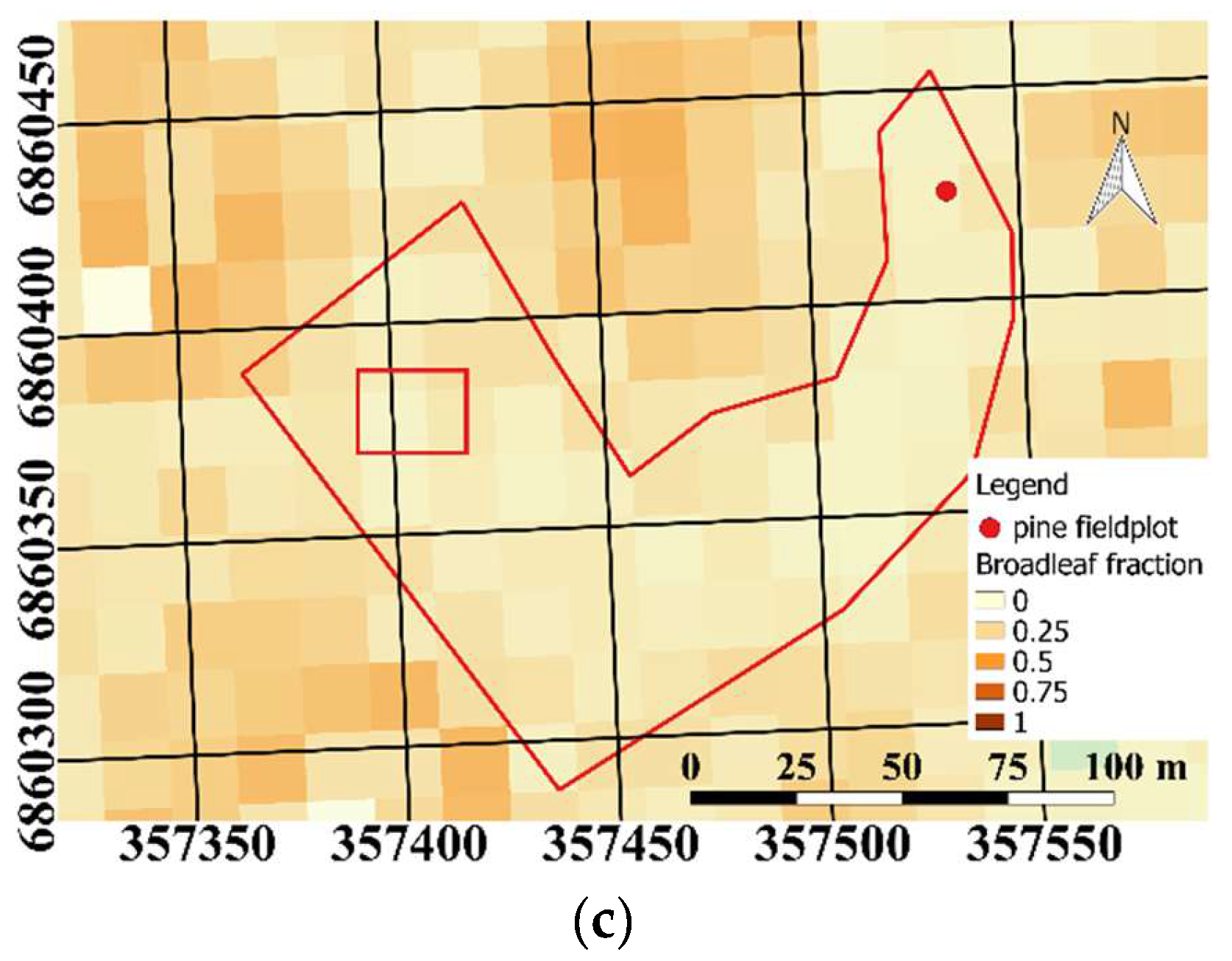
We manually selected the study plot (Figure 2a) using raster maps of biomass by tree species (Pine: Figure 2b and broadleaf: Figure 2c) from the National Forest Inventory for 2013 (MS-NFI, © Natural Resources Institute Finland, Helsinki, Finland, 2015). We selected a visually homogeneous polygon in the AHS imagery where we had a Scots pine biomass fraction of at least 50%; no spruce was present in the study plot. Scots pine and silver birch can easily be visually distinguished from Figure 2a, as broadleaf trees have a considerably higher near infrared (NIR) reflectance than Scots pine, and hence look red in the false color figure. The study plot covered 1.2 hectares, and included approximately 35,690 AHS pixels. During field measurements in 2011, the plot had been classified as a young mesic pure Scots pine stand with 84% canopy cover and effective LAI = 2.7 (Figure 2a). The study site had not been subjected to any harvesting or other abrupt changes. Considering the slow growth of forests in this region, the measured LAI value can be used to characterize the plot with reasonable accuracy still in 2015.
We then masked out all non-vegetative pixels, such as bare soil, in ENVI (Harris Geospatial Solutions, Broomfield, CO, USA) using a normalized difference vegetation index (NDVI) threshold of 0.8 (Table 3). This threshold successfully retained most of the vegetative pixels while removing only clearly non-vegetated ones. The number of pixels masked out was less than 8% in the nadir direction, and less than 1% for the off-nadir directions (Table 3).
2.4. Spectral Similarity Metrics
To test the spectral similarity between Scots pine canopy sunlit fraction pixels observed from different view angles, we used the spectral information divergence measure (SID) [30]. SID is the discrepancy of the probability distribution between two spectral vectors. Van der Meer [31] has tested several common spectral similarity algorithms using synthetic and measured Airborne Visible/Infrared Imaging Spectrometer (AVIRIS) data. They concluded that SID is more effective in mapping and detecting targets, and is less sensitive to spectral noise compared with other tested spectral metrics.
2.5. Calculation of Canopy PRI
We calculated the Scots pine canopy PRI for each scatter angle using the spectral central wavelengths at 533 nm and 569 nm closest to the PRI wavelengths 531 nm and 570 nm. We used a standard t-test to determine whether the mean PRI for each flight line was statistically significantly different to each other.
2.6. Scots Pine Canopy Sunlit Fraction Retrieval
First, we fitted the equation:
to the AHS data with band centers between 711 nm to 787 nm, where and p are two constants [32,33] known as the directional escape and recollision probabilities, respectively. For the leaf albedo , we used the synthetic leaf reference albedo calculated with the PROSPECT-4 leaf optical properties model [34], with the parameters set to the optimal values for the method as prescribed by Knyazikhin et al. [32,33]: leaf dry matter content , chlorophyll a and b content , leaf water content . The parameter is related to the sunlit fraction described by Hernández-Clemente et al. [35]:
where is the solar zenith angle. However, the sunlit fraction depends on the scale of the scattering element (e.g., shoot, needle, or a within-needle structure [36]) that the single-scattering albedo belongs to. The transformed albedos of green foliage of different structural levels follow a simple scaling rule:
or
where the recollision probability quantifies the probability of the event that a photon scattered by the object residing in (e.g., needle in the shoot) will interact within again (e.g., hit another needle within the same shoot) (Equation (2) by Knyazikhin et al. in [33], originally derived by Smolander and Stenberg [37]). More generally, Equation (3) can be used to connect any two leaf albedos [32]. We used the Scots pine needle albedo measured in Hyytiälä [36] transformed to correct for gap fractions and specular reflectance. By setting and in Equation (3), and applying a linear regression, we found that is related to as:
or, .
As both and in Equation (3) can be used to form a relationship with BRDF identical to Equation (1), we obtain the following scaling equations for the parameters p and :
Now, we can write Hence, we could convert the sunlit fraction obtained with the reference albedo in Equation (2), to the fraction of sunlit Scots pine needles , hereafter denoted as , by dividing by 0.648.
We used the IDL programming language and ENVI (Harris Geospatial Solutions, USA) software to fit Equation (1) to AHS data and to create maps for all three flight lines. In the place of BRDF, we used the AHS-measured HDRF values. In the red edge spectral region, and especially on a clear day, the difference between HDRF and BRDF is very small.
Under the assumption of the sunlit fraction being the main driver of the spectral shape of BRDF, we extracted Scots pine canopy BRDF in seven ranges and evaluated the similarity of the BRDFs using the SID algorithm. We inspected sunlit fraction histograms to find the smallest sunlit fraction value ranges with more than 80 pixels for each view angle. We selected the following intervals: , , , , , , . (Table 4). We averaged the spectra in each interval to obtain 16 Scots pine canopy reflectance spectra, specific to each view angle and interval. Note that the data for each interval were not always available due to the natural range of (Table 4).
2.7. Dependence of PRI on Sunlit Fraction
The dependence of the remotely measured PRI on the sunlit fraction (assuming all other factors, including leaf optical properties, constant) is given by Equation (9) by Barton and North [18] as:
where is the spectral irradiance on leaf surface at the wavelength , and is the TOC spectral irradiance on a horizontal surface. We can divide the spectral irradiance into the diffuse and direct components denoted with the superscripts dif and dir, respectively, i.e., . We used the approximation of the direct and diffuse irradiances on needle surfaces proposed by Mõttus et al. [29] (Equation (11)):
where is the ratio of average projected area of the element in the direction given by the solar zenith angle , and is the average fraction of diffuse sky radiation reaching the visible leaves. For broadleaves, ; for an isotropic distribution of leaf (or needle) normals, . Hence, we get:
According to Equation (8), the remotely measured PRI thus consists of a part determined by leaf optical properties and incident illumination conditions:
and a part depending on . For completely shaded leaves (), . The range of PRI variation with is thus determined as:
where is the value of PRI at . Mõttus et al. [29] assumed , as this parameter cannot be measured directly. Hence, we bundled the various coefficients into parameters that we retrieved from remotely sensed data.
We used the non-linear regression line fitting function prediction in the R statistical software environment (version 1.0.136), to make a prediction between the Scots pine canopy sunlit fraction and the Scots pine canopy PRI for each scatter angle. We used the equation:
where is the value of PRI at ; and and are curve parameters that depend on the irradiance ratios, , and the solar angle.
3. Results
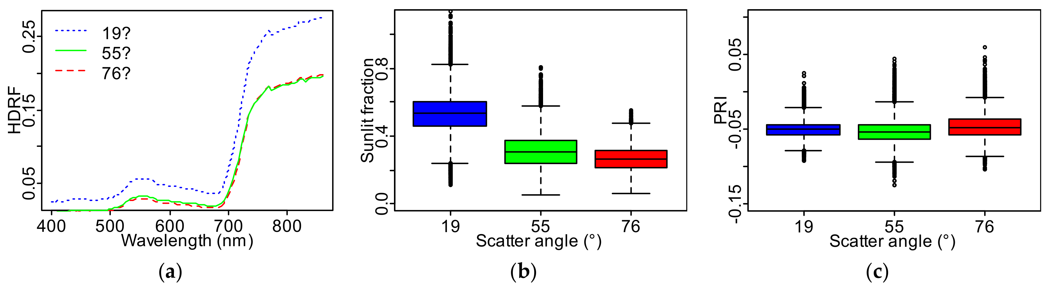
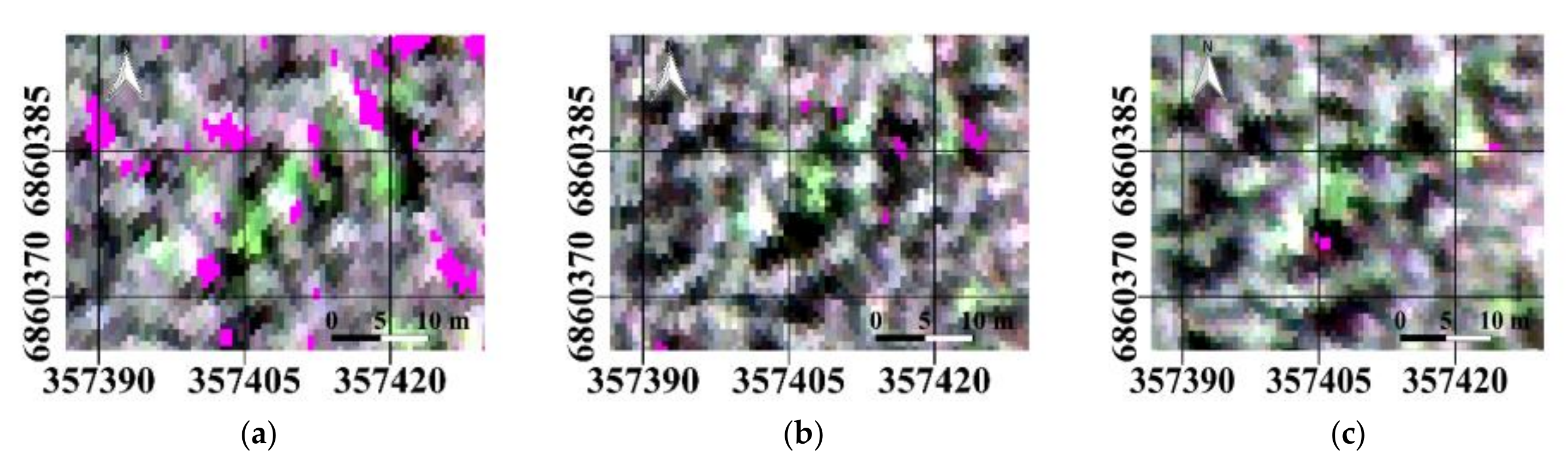
The average Scots pine TOC reflectance was approximately the same for the scatter angles ° and 90°, with significantly higher values produced across the spectrum at °, the direction closest to hot spot (Figure 3a). This trend is mirrored in the fraction of sunlit needles for the three view angles (Figure 3b): the average sunlit fraction decreased as the scatter angle increased, but the difference in (0.04) between scatter angles 55° and 76° was smaller than between 19° and 55° (0.21), although all differences in scatter angles were significant (p << 0.01). Mean PRI, on the other hand, did not change monotonically with the scatter angle (Figure 3c). The smallest PRI value of −0.052 was measured for near-nadir direction (°) with near-similar values of −0.049 and −0.046 for the scatter angles ° and °, respectively. Despite the overlapping ranges in Figure 3c, t-tests indicated a significant difference (p < 0.01) between the PRI values for three lines. The range of the within-view angle in PRI varied with the scatter angle from 0.117 at °, to 0.169 at °, and 0.163 at °. The standard deviation in PRI was 0.011 at °, 0.162 at °, and 0.158 at °. A true color image of the focus area highlights the spatial variation in Scots pine canopy brightness for all three scatter angles (Figure 4). The spatial variation in PRI (Figure 5) and sunlit fraction (Figure 6) were also visually compared for all three scatter angles.
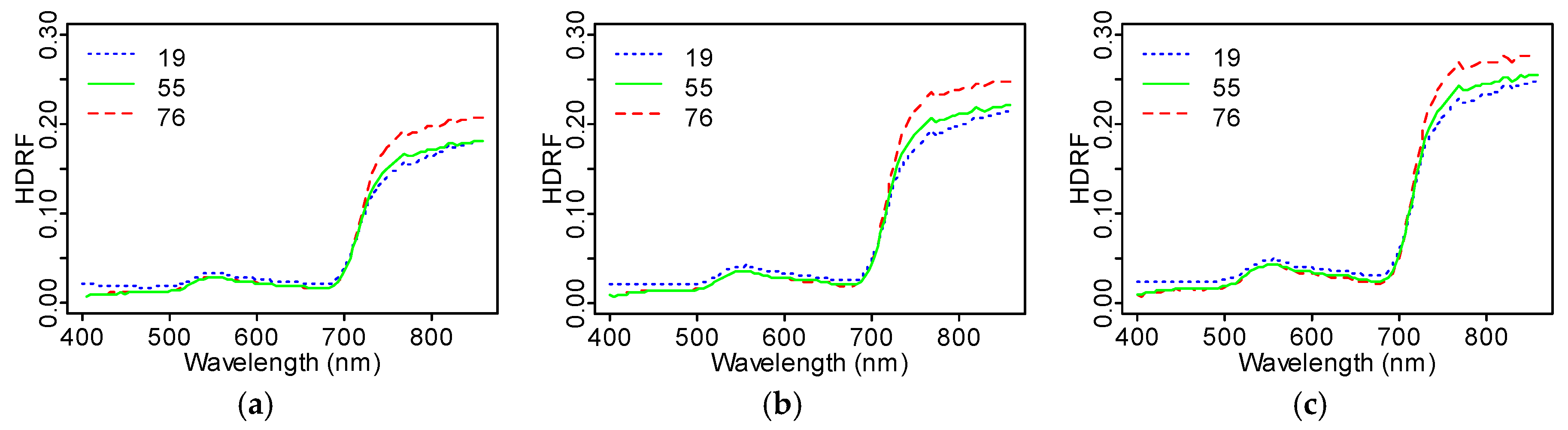
The scatter angle closest to the hot spot (β = 19°) produced higher average TOC HDRF values than scatter angles 55° and 76° in the visible region (400–700 nm), but less reflectance in the near-infrared region (700–870 nm) (Figure 7) for any fixed interval of the sunlit fraction . To investigate this, we divided the average TOC HDRF reflectance at the oblique angles (° and °) by the reflectance close to nadir (°). We observed a general decrease in the HDRF (19°)/HDRF (55°) ratio with , with especially strong dependence in the visible wavelengths. The ratio HDRF (76°)/HDRF (55°) remained more constant and was close to unity across the whole measured spectrum (Figure 8). In both cases (HDRF (19°)/HDRF (55°) and HDRF (76°)/HDRF (55°)), the highest HDRF ratio values were obtained for between 0.43 and 0.45.
We compared spectral divergence for all sunlit fraction ranges given in Table 4. The largest SID (0.019) for within flight line was observed when the distance between two sunlit fraction ranges 0.06–0.08 vs. 0.43–0.45 (Figure 9). We observed this pattern for each flight line, with somewhat smaller average SID values across the whole range of observed for 19° (Figure 9).
We also compared the SID of HDRFs for all sunlit fraction intervals in Table 4 between the three scatter angles. We observed the largest spectral divergence (SID = 0.037) between and 76° for (Table 5). The smallest SID (0.001) was observed between 55° and 76°. Scatter angles 55° and 76° produced the lowest SID values for all of the sunlit fraction ranges, with 0.003 the highest SID value for . In contrast, the lowest SID value for 19° vs. 55° and 19° vs. 76° were 0.017 and 0.033, respectively. The SID values for all of the sunlit fractions were the smallest for 55° vs. 76°.
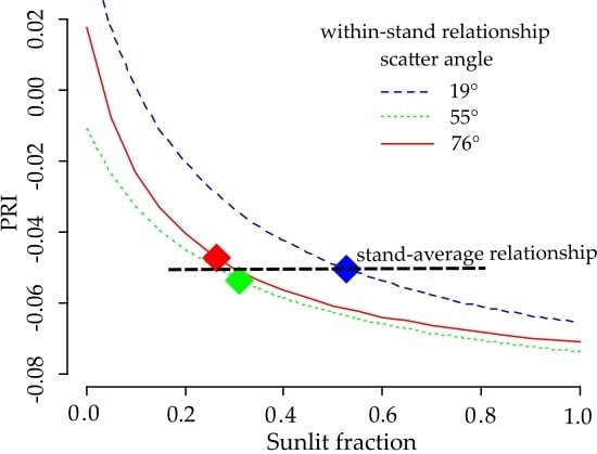
The parameters of the non-linear regression model (Figure 10) of PRI as a function of sunlit fraction are given in Table 6. The dependence of PRI on sunlit fraction becomes stronger as the scatter angle increases. This dependence is visible when all of the data is combined, and results in a steeper curve for small sunlit fraction values () (Figure 10d). A comparison of the four fitted lines in Figure 11 shows that the curves for the three scatter angles are quasi-parallel, and are intersected by the curve fitted to all data.
4. Discussion
Kuusk et al. [38] have measured canopy reflectance in Järvselja at two wavelengths (660 nm and 850 nm) at a solar zenith angle of 52° at 660 nm, and a solar zenith angle of 46° at 850 nm. In the 660 nm wavelength band, they reported HDRF values of 0.03, 0.02, and 0.02 for , , and , respectively. Our values, measured in Hyytiälä, were 0.03, 0.02, and 0.02, respectively. In the 850 nm wavelength band, the HDRF values in Järvselja were 0.18, 0.15, and 0.12 [38] for scatter angles of 19°, 55°, and 76°, respectively. The corresponding values obtained by us in Hyytiälä were 0.27, 0.19, and 0.19. The values are remarkably similar in the red band. The difference in canopy HDRF in the NIR region (850 nm) is likely due to different canopy structures and illumination angles. The dark spot (lowest HDRF) observed by Kuusk et al. [38] was approximately 25° off-nadir, which is close to the observation geometry used in the study: with good approximation, we can consider to represent the dark spot of the canopy.
We found a strong non-linear relationship between canopy PRI and sunlit fraction for each view angle separately. The relationships could be modeled with the equations provided by Mõttus et al. [29]. Our empirical findings support that the observed fraction of canopy shadow in the field of view of the sensor is an important driver for spectral BRDF. Further, the dependence between sunlit (or shadow) fraction and PRI is strongly non-linear, and the linear model that has been used by many authors [20,27,39] should be used with care. However, is not the only, or not necessarily even the key driver in scattering directionality. The observed maximum spectral divergence among the vegetated pixels caused by for any fixed scatter angle was 0.02 (Figure 9). At a constant , we observed much larger spectral divergence values (Table 5). While the two darkest view angles ( and ) were relatively similar (maximum divergence 0.03), the angle closest to the hot spot () differed from the other two, with maximum SID values close to 0.04.
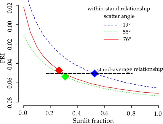
The relationship between and the PRI was the strongest at , and flattened out when sunlit fraction increased. The mean values for the three view angles were close to or above this threshold. Despite the strong relationship between and the PRI for each view angle separately, the stand mean PRI did not change systematically with the scatter angle. As the PRI— curves for the three view angles were quasi-parallel with similar parameters (Table 6), the location of on the flat part of the curve made the PRI sensitive to other potential interfering factors. The difference between the curves for the three view angles, caused by an unspecified factor, was systematic and apparently independent from (Figure 11). When we combined all of the PRI and sunlit fraction values for all of the scatter angles (Figure 11), the curve was not parallel to the other curves. Further, the curve did not approach a meaningful value at Unrealistic values were also retrieved for other model parameters (Table 6). These results indicate the existence of another factor besides that depends on scatter angle and affects PRI systematically and across all values.
When canopy reflectance would be averaged over all vegetation pixels (e.g., to simulate the signal of a medium spatial resolution sensor over a closed canopy), this unspecified factor would dominate over by eliminating the dependence of PRI on the sunlit fraction . Although the masks that were used to exclude non-vegetated pixels were different for each scatter angle, not applying a mask (i.e., a true simulation of large-footprint sensor) would not alter the dependence of PRI on in Figure 3 (data not shown). The masks did not differentiate between the tree species growing in the test site. According to the raster maps from the National Forest Inventory, a small fraction of birch trees were expected at the site. However, based on visual inspection of the AHS images (Figure 2), the presence of broadleaf was small, and the effect on the PRI–shadow fraction analysis can be neglected.
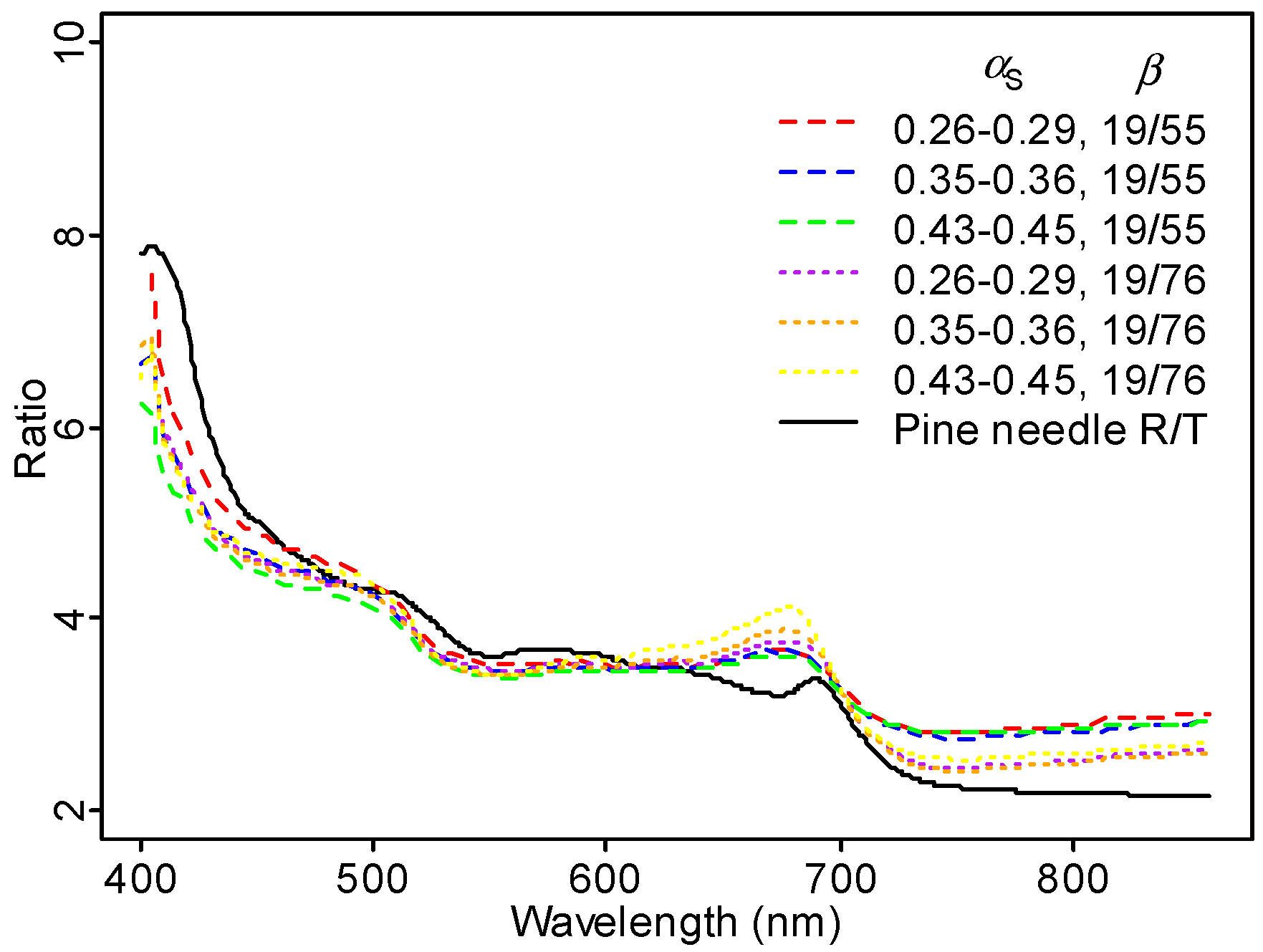
When we compared the ratio of Scots pine TOC reflectance between the direction closest to hot spot () and nadir () for different sunlit fractions, we observed a high value, especially in the blue region (Figure 8). We hypothesize that this is caused by needle wax [40]. In the visible wavelengths where leaf pigments are highly absorbing, leaf scattering is dominated by specular reflectance at the surface [41]. Specular reflectance, directed mostly in backward directions, increases strongly with decreasing wavelength in the visible spectral region. To test this, we plotted the ratio of Scots pine needle reflectance to transmittance measured in Hyytiälä in 2013 [42], and observed a pattern similar with our observed ratio between TOC reflectance for two scatter angles (Figure 12).
The variation in leaf reflectance to transmittance ratio in Figure 12 explains the unexpectedly large PRI close to hot spot well. When calculated from laboratory-measured needle transmittance, Scots pine needle PRI in midsummer 2012 was −0.008; when calculated from reflectance, PRI was 0.014. In the hot spot direction, canopy reflectance in the visible part of the spectrum (where multiple scattering can be ignored to a reasonable accuracy) is contributed by reflectance only, while in the dark spot, both needle reflectance and transmittance contribute. The two measurements (laboratory measurements of needle spectra and AHS data) cannot be compared directly, as laboratory-measured data are directional–hemispherical, and airborne data hemispherical–directional. However, the two curves show similar features: a local minimum at 550 nm and a local maximum close to 680 nm. The importance of specular scattering in Scots pine canopies is not unexpected. In the laboratory, Mõttus and Rautiainen [43] have shown that shoot scattering directionality needs to be accounted for when interpreting multi-angular PRI measurements, and that the directionality is likely caused by specular scattering. Obviously, this statement is not only valid for the relatively exotic airborne multi-angular imaging spectroscopy data, but also whenever angular information is applied on spectral remote sensing data, e.g., fitting BRDF models or correcting for angular effects in instruments with wide swaths, and analysis of tower-based PRI measurements. Moreover, the specific structural effects described here need to be accounted for when comparing nadir measurements made at different solar angles, such as for example when analyzing the time series of data from a single location measured from a sun-synchronous satellite.
We have demonstrated the applicability of a simple PRI— model for constant view geometry and the dependence of this relationship on the scattering directionality of leaves (needles). This model can be used to eliminate the non-physiological effects in the measured PRI signal, and connect observed PRI variations with shadow fraction—either in multi-angular or high spatial resolution data—to variations in photosynthetic activity. More work is required to quantify these relationships and relate stand scattering characteristics with atmospheric variables and leaf structural information. Without a physical model, canopy level spectral information cannot be robustly linked to the physiological processes taking place in leaves.
5. Conclusions
We were able to model the PRI–sunlit fraction relationship measured from multi-angular imaging spectroscopy data. The relationship is strongly non-linear, and PRI is less sensitive to sunlit fraction when sunlit crown pixels dominate the sensor’s field of view. Furthermore, the relationship depends on observation angle, likely because of specular reflectance from needle surfaces. Consequently, mean TOC PRI was not monotonically linked with scatter angle and sunlit fraction, despite a strong monotonic dependence of PRI on sunlit (or shadow) fraction for each scatter angle separately. In other words, we found that (a lack of) TOC dependence of PRI on sunlit fraction obtained from multi-angular measurements need not indicate (a lack of) a dependence of TOC PRI on sunlit fraction under fixed observation geometry. Identification of the two causal mechanisms of non-physiological PRI dependence on sunlit fraction presented in the current manuscript contributes towards the development of robust algorithms for scaling canopy PRI to leaf level for the monitoring of forest productivity.
Acknowledgments
This study and its publication were funded by the Academy of Finland (grants 266152, 272989 and 303633). We are grateful to Lauri Korhonen (University of Eastern Finland) for providing the field data of the test stand and to MSc Viljami Perheentupa for valuable technical assistance and comments.
Author Contributions
Matti Mõttus and Rocío Hernández-Clemente conceived and designed the experiments; Vincent Markiet preprocessed and analyzed the data; Vincent Markiet and Matti Mõttus wrote the paper.
Conflicts of Interest
The authors declare no conflict of interest.
References
- Keenan, R.J.; Reams, G.A.; Achard, F.; de Freitas, J.V.; Grainger, A.; Lindquist, E. Dynamics of global forest area: Results from the FAO Global Forest Resources Assessment 2015. For. Ecol. Manag. 2015, 352, 9–20. [Google Scholar] [CrossRef]
- Pan, Y.; Birdsey, R.A.; Fang, J.; Houghton, R.; Kauppi, P.E.; Kurz, W.A.; Phillips, O.L.; Shvidenko, A.; Lewis, S.L.; Canadell, J.G.; et al. A large and persistent carbon sink in the world’s forests. Science 2011, 333, 988–993. [Google Scholar] [CrossRef] [PubMed]
- Gibbs, H.K.; Brown, S.; Niles, J.; Foley, J. Monitoring and estimating tropical forest carbon stocks: Making REDD a reality. Environ. Res. Lett. 2007, 2. [Google Scholar] [CrossRef]
- Goetz, S.J.; Baccini, A.; Laporte, N.T.; Johns, T.; Walker, W.; Kellndorfer, J.; Houghton, R.A.; Sun, M. Mapping and monitoring carbon stocks with satellite observations: A comparison of methods. Carbon Balance Manag. 2009, 4. [Google Scholar] [CrossRef] [PubMed]
- Drusch, M.; Del Bello, U.; Carlier, S.; Colin, O.; Fernandez, V.; Gascon, F.; Hoersch, B.; Isola, C.; Laberinti, P.; Martimort, P.; et al. Sentinel-2: ESA’s Optical High-Resolution Mission for GMES Operational Services. Remote Sens. Environ. 2012, 120, 25–36. [Google Scholar] [CrossRef]
- Drusch, M.; Moreno, J.; Del Bello, U.; Franco, R.; Goulas, Y.; Huth, A.; Kraft, S.; Middleton, E.M.; Miglietta, F.; Mohammed, G.; et al. The FLuorescence EXplorer Mission Concept—ESA’s Earth Explorer 8. IEEE Trans. Geosci. Remote Sens. 2017, 55, 1273–1284. [Google Scholar] [CrossRef]
- Gitelson, A.A.; Gamon, J.A. The need for a common basis for defining light-use efficiency: Implications for productivity estimation. Remote Sens. Environ. 2015, 156, 196–201. [Google Scholar] [CrossRef]
- Monteith, J.L.; Moss, C.J. Climate and the Efficiency of Crop Production in Britain [and Discussion]. Philos. Trans. R. Soc. London B 1977, 281, 277–294. [Google Scholar] [CrossRef]
- Delucia, E.H.; Gomez-Casanovas, N.; Greenberg, J.A.; Hudiburg, T.W.; Kantola, I.B.; Long, S.P.; Miller, A.D.; Ort, D.R.; Parton, W.J. The theoretical limit to plant productivity. Environ. Sci. Technol. 2014, 48, 9471–9477. [Google Scholar] [CrossRef] [PubMed]
- Gamon, J.A.; Field, C.B.; Fredeen, A.L.; Thayer, S. Assessing photosynthetic downregulation in sunflower stands with an optically-based model. Photosynth. Res. 2001, 67, 113–125. [Google Scholar] [CrossRef] [PubMed]
- Hilker, T.; Hall, F.G.; Tucker, C.J.; Coops, N.C.; Black, T.A.; Nichol, C.J.; Sellers, P.J.; Barr, A.; Hollinger, D.Y.; Munger, J.W. Data assimilation of photosynthetic light-use efficiency using multi-angular satellite data: II Model implementation and validation. Remote Sens. Environ. 2012, 121, 287–300. [Google Scholar] [CrossRef]
- Demmig-Adams, B.; Adams, W.W. The role of xanthophyll cycle carotenoids in the protection of photosynthesis. Trends Plant Sci. 1996, 1, 21–26. [Google Scholar] [CrossRef]
- Gamon, J.A.; Peñuelas, J.; Field, C.B. A narrow-waveband spectral index that tracks diurnal changes in photosynthetic efficiency. Remote Sens. Environ. 1992, 41, 35–44. [Google Scholar] [CrossRef]
- Wong, C.Y.S.; Gamon, J.A. Three causes of variation in the photochemical reflectance index (PRI) in evergreen conifers. New Phytol. 2015, 206, 187–195. [Google Scholar] [CrossRef] [PubMed]
- Peguero-Pina, J.J.; Morales, F.; Flexas, J.; Gil-Pelegrín, E.; Moya, I. Photochemistry, remotely sensed physiological reflectance index and de-epoxidation state of the xanthophyll cycle in Quercus coccifera under intense drought. Oecologia 2008, 156. [Google Scholar] [CrossRef] [PubMed]
- Gitelson, A.A.; Gamon, J.A.; Solovchenko, A.E. Multiple drivers of seasonal change in PRI : Implications for photosynthesis 1. Remote Sens. Environ. 2017, 191, 110–116. [Google Scholar] [CrossRef]
- Peñuelas, J.; Filella, I.; Gamon, J.A. Assessment of photosynthetic radiation-use efficiency with spectral reflectance. New Phytol. 1995, 131. [Google Scholar] [CrossRef]
- Barton, C.V.M.; North, P.R.J. Remote sensing of canopy light use efficiency using the photochemical reflectance index. Model and sensitivity analysis. Remote Sens. Environ. 2001, 78, 264–273. [Google Scholar] [CrossRef]
- Hernández-Clemente, R.; Navarro-Cerrillo, R.M.; Suárez, L.; Morales, F.; Zarco-Tejada, P.J. Assessing structural effects on PRI for stress detection in conifer forests. Remote Sens. Environ. 2011, 115, 2360–2375. [Google Scholar] [CrossRef]
- Takala, T.L.H.; Mõttus, M. Spatial variation of canopy PRI with shadow fraction caused by leaf-level irradiation conditions. Remote Sens. Environ. 2016, 182, 99–112. [Google Scholar] [CrossRef]
- Schickling, A.; Matveeva, M.; Damm, A.; Schween, J.H.; Wahner, A.; Graf, A.; Crewell, S.; Rascher, U. Combining sun-induced chlorophyll fluorescence and photochemical reflectance index improves diurnal modeling of gross primary productivity. Remote Sens. 2016, 8. [Google Scholar] [CrossRef]
- Chen, J.M.; Menges, C.H.; Leblanc, S.G. Global mapping of foliage clumping index using multi-angular satellite data. Remote Sens. Environ. 2005, 97, 447–457. [Google Scholar] [CrossRef]
- Chen, J.M.; Leblanc, S.G. Multiple-scattering scheme useful for geometric optical modeling. IEEE Trans. Geosci. Remote Sens. 2001, 39, 1061–1071. [Google Scholar] [CrossRef]
- Nichol, C.J.; Lloyd, J.; Shibistova, O.; Arneth, A.; Röser, C.; Knohl, A.; Matsubara, S.; Grace, J. Remote sensing of photosynthetic-light-use efficiency of a Siberian boreal forest. Tellus Ser. B 2002, 54, 677–687. [Google Scholar] [CrossRef]
- Filella, I.; Porcar-Castell, A.; Munné-Bosch, S.; Bäck, J.; Garbulsky, M.F.; Peñuelas, J. PRI assessment of long-term changes in carotenoids/chlorophyll ratio and short-term changes in de-epoxidation state of the xanthophyll cycle. Int. J. Remote Sens. 2009, 30, 4443–4455. [Google Scholar] [CrossRef]
- Nakaji, T.; Ide, R.; Takagi, K.; Kosugi, Y.; Ohkubo, S.; Nasahara, K.N.; Saigusa, N.; Oguma, H. Utility of spectral vegetation indices for estimation of light conversion efficiency in coniferous forests in Japan. Agric. For. Meteorol. 2008, 148, 776–787. [Google Scholar] [CrossRef]
- Hall, F.G.; Hilker, T.; Coops, N.C.; Lyapustin, A.; Huemmrich, K.F.; Middleton, E.; Margolis, H.; Drolet, G.; Black, T.A. Multi-angle remote sensing of forest light use efficiency by observing PRI variation with canopy shadow fraction. Remote Sens. Environ. 2008, 112, 3201–3211. [Google Scholar] [CrossRef]
- Hilker, T.; Coops, N.C.; Hall, F.G.; Black, T.A.; Wulder, M.A.; Nesic, Z.; Krishnan, P. Separating physiologically and directionally induced changes in PRI using BRDF models. Remote Sens. Environ. 2008, 112, 2777–2788. [Google Scholar] [CrossRef]
- Mõttus, M.; Takala, T.L.H.; Stenberg, P.; Knyazikhin, Y.; Yang, B.; Nilson, T. Diffuse sky radiation influences the relationship between canopy PRI and shadow fraction. ISPRS J. Photogramm. Remote Sens. 2015, 105, 54–60. [Google Scholar] [CrossRef]
- Chang, C. An information-theoretic approach to spectral variability, similarity, and discrimination for hyperspectral image analysis. IEEE Trans. Inf. Theory 2000, 46, 1927–1932. [Google Scholar] [CrossRef]
- Van der Meer, F. The effectiveness of spectral similarity measures for the analysis of hyperspectral imagery. Int. J. Appl. Earth Obs. Geoinf. 2006, 8, 3–17. [Google Scholar] [CrossRef]
- Knyazikhin, Y.; Schull, M.A.; Stenberg, P.; Mõttus, M.; Rautiainen, M.; Yang, Y.; Marshak, A.; Latorre Carmona, P.; Kaufmann, R.K.; Lewis, P.; et al. Hyperspectral remote sensing of foliar nitrogen content. Proc. Natl. Acad. Sci. USA 2013, 110, E185–E192. [Google Scholar] [CrossRef] [PubMed]
- Knyazikhin, Y.; Schull, M.A.; Xu, L.; Myneni, R.B.; Samanta, A. Canopy spectral invariants. Part 1: A new concept in remote sensing of vegetation. J. Quant. Spectrosc. Radiat. Transf. 2011, 112, 727–735. [Google Scholar] [CrossRef]
- Feret, J.B.; François, C.; Asner, G.P.; Gitelson, A.A.; Martin, R.E.; Bidel, L.P.R.; Ustin, S.L.; le Maire, G.; Jacquemoud, S. PROSPECT-4 and 5: Advances in the leaf optical properties model separating photosynthetic pigments. Remote Sens. Environ. 2008, 112, 3030–3043. [Google Scholar] [CrossRef]
- Hernández-Clemente, R.; Kolari, P.; Porcar-Castell, A.; Korhonen, L.; Mõttus, M. Tracking the Seasonal Dynamics of Boreal Forest Photosynthesis Using EO-1 Hyperion Reflectance: Sensitivity to Structural and Illumination Effects. IEEE Trans. Geosci. Remote Sens. 2016, 54, 5105–5116. [Google Scholar] [CrossRef]
- Lewis, P.; Disney, M. Spectral invariants and scattering across multiple scales from within-leaf to canopy. Remote Sens. Environ. 2007, 109, 196–206. [Google Scholar] [CrossRef]
- Smolander, S.; Stenberg, P. A method to account for shoot scale clumping in coniferous canopy reflectance models. Remote Sens. Environ. 2003, 88, 363–373. [Google Scholar] [CrossRef]
- Kuusk, A.; Kuusk, J.; Lang, M. Measured spectral bidirectional reflection properties of three mature hemiboreal forests. Agric. For. Meteorol. 2014, 185, 14–19. [Google Scholar] [CrossRef]
- Soudani, K.; Hmimina, G.; Dufrêne, E.; Berveiller, D.; Delpierre, N.; Ourcival, J.-M.; Rambal, S.; Joffre, R. Relationships between photochemical reflectance index and light-use efficiency in deciduous and evergreen broadleaf forests. Remote Sens. Environ. 2014, 144, 73–84. [Google Scholar] [CrossRef]
- Nilson, T.; Ross, J. Modeling Radiative Transfer through Forest Canopies: Implications for Canopy Photosynthesis and Remote Sensing. In The Use of Remote Sensing in the Modeling of Forest Productivity; Shimoda, H., Gholz, H.L., Nakane, K., Eds.; Springer: Dordrecht, The Netherlands, 1997; pp. 23–60. ISBN 978-94-011-5446-8. [Google Scholar]
- Grant, L. Diffuse and specular characteristics of leaf reflectance. Remote Sens. Environ. 1987, 22, 309–322. [Google Scholar] [CrossRef]
- Lukeš, P.; Stenberg, P.; Rautiainen, M.; Mõttus, M.; Vanhatalo, K.M. Optical properties of leaves and needles for boreal tree species in Europe. Remote Sens. Lett. 2013, 4, 667–676. [Google Scholar] [CrossRef]
- Mõttus, M.; Rautiainen, M. Scaling PRI between coniferous canopy structures. IEEE J. Sel. Top. Appl. Earth Obs. Remote Sens. 2013, 6, 708–714. [Google Scholar] [CrossRef]
Figure 1.
Hyperspectral AISA Eagle II sensor and IMU system on a tilting platform looking in the nadir direction through the cargo bay entrance at the rear of the aircraft. The cables connecting the instruments have been removed for better visibility. We configured the sensor to scan with a 60 Hz framerate. The chosen configuration resulted in square pixels of approximately 60 cm for nadir view; in off-nadir directions, the pixels were slightly elongated (Table 1). Full technical characteristics of the sensor are given in Table 2.
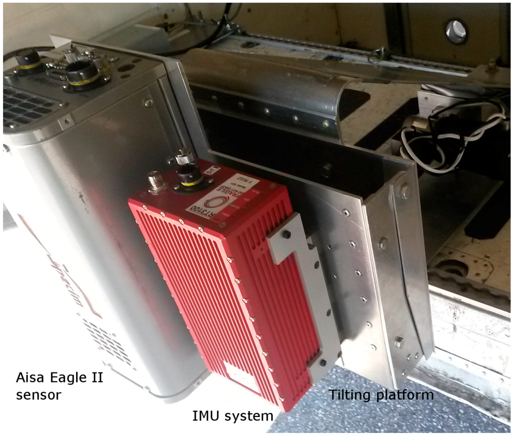
Figure 2.
(a) A false color (red: 858 nm, green: 649 nm, blue: 547 nm) image of the selected Scots pine plot marked by the red border; (b) Scots pine biomass fraction map; (c) Broadleaf biomass fraction map. The red dot marks the field plot measured in 2011.
Figure 2.
(a) A false color (red: 858 nm, green: 649 nm, blue: 547 nm) image of the selected Scots pine plot marked by the red border; (b) Scots pine biomass fraction map; (c) Broadleaf biomass fraction map. The red dot marks the field plot measured in 2011.
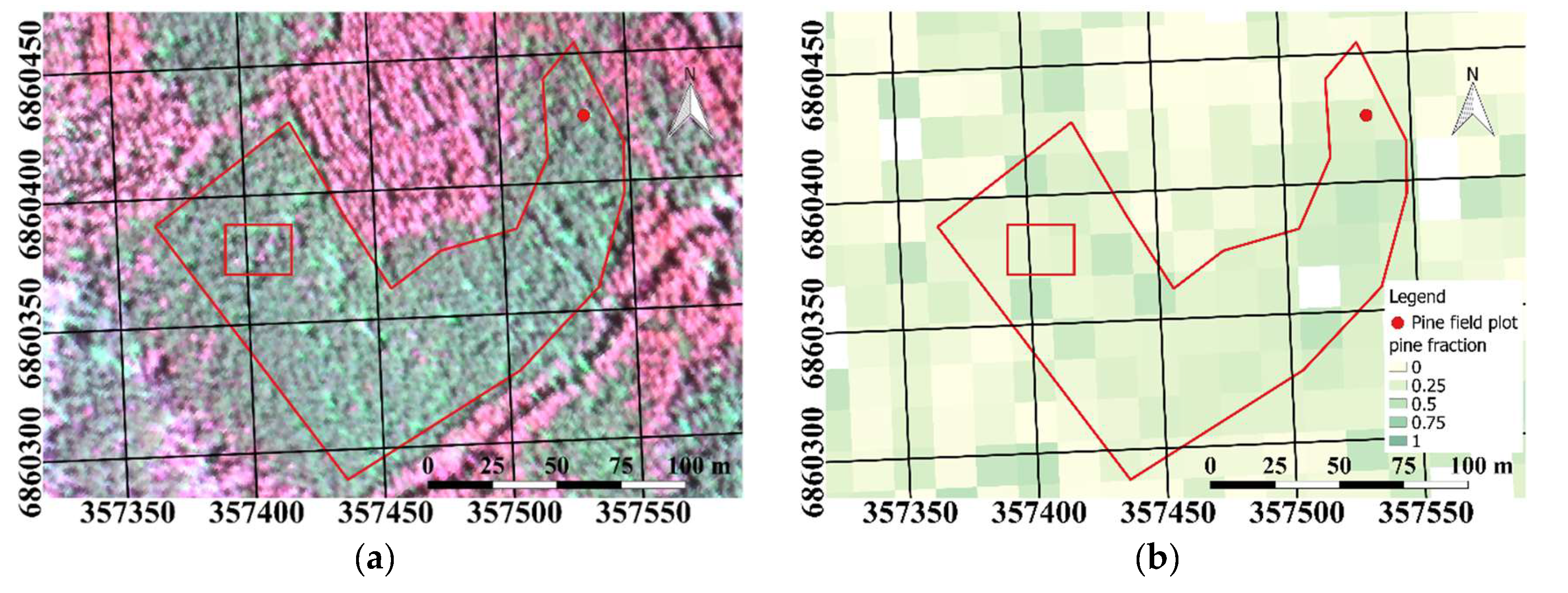

Figure 3.
Average Scots pine top of canopy (TOC) spectral reflectance (a), Scots pine canopy sunlit fraction (b) and Scots pine canopy photochemical reflectance index (PRI) (c) for three scatter angles ( 19°, 55° and 76°).
Figure 3.
Average Scots pine top of canopy (TOC) spectral reflectance (a), Scots pine canopy sunlit fraction (b) and Scots pine canopy photochemical reflectance index (PRI) (c) for three scatter angles ( 19°, 55° and 76°).

Figure 4.
True color images of the focus area (red rectangle in Figure 2) inside the test polygon showing spatial variation in Scots pine canopy brightness for different scatter angles ( 19° (a); 55° (b); 76° (c)). Purple pixels were masked out; normalized difference vegetation index (NDVI) < 0.8.
Figure 4.
True color images of the focus area (red rectangle in Figure 2) inside the test polygon showing spatial variation in Scots pine canopy brightness for different scatter angles ( 19° (a); 55° (b); 76° (c)). Purple pixels were masked out; normalized difference vegetation index (NDVI) < 0.8.

Figure 5.
Spatial variation of the canopy PRI for 19° (a); 55° (b); and 76° (c). Purple pixels were masked out (NDVI < 0.8). The color scale is the same for all three rasters.
Figure 5.
Spatial variation of the canopy PRI for 19° (a); 55° (b); and 76° (c). Purple pixels were masked out (NDVI < 0.8). The color scale is the same for all three rasters.
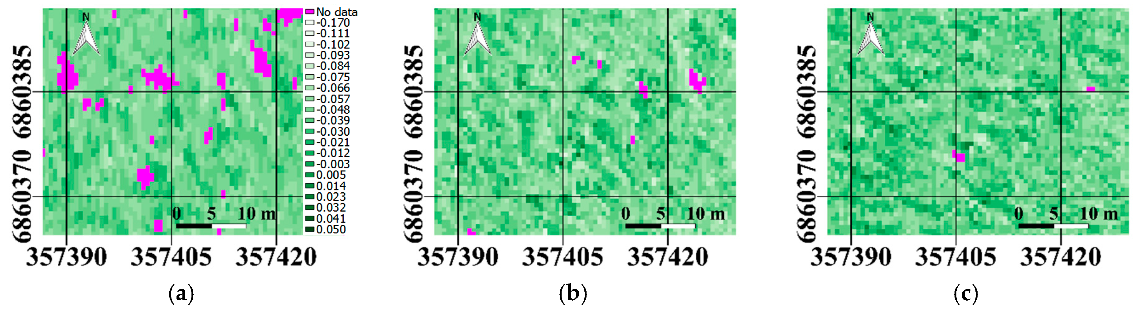
Figure 6.
Spatial variation of the canopy sunlit fraction for 19° (a), 55° (b), 76° (c). Purple pixels were masked out (NDVI < 0.8). The color scale is the same for all three rasters.
Figure 6.
Spatial variation of the canopy sunlit fraction for 19° (a), 55° (b), 76° (c). Purple pixels were masked out (NDVI < 0.8). The color scale is the same for all three rasters.
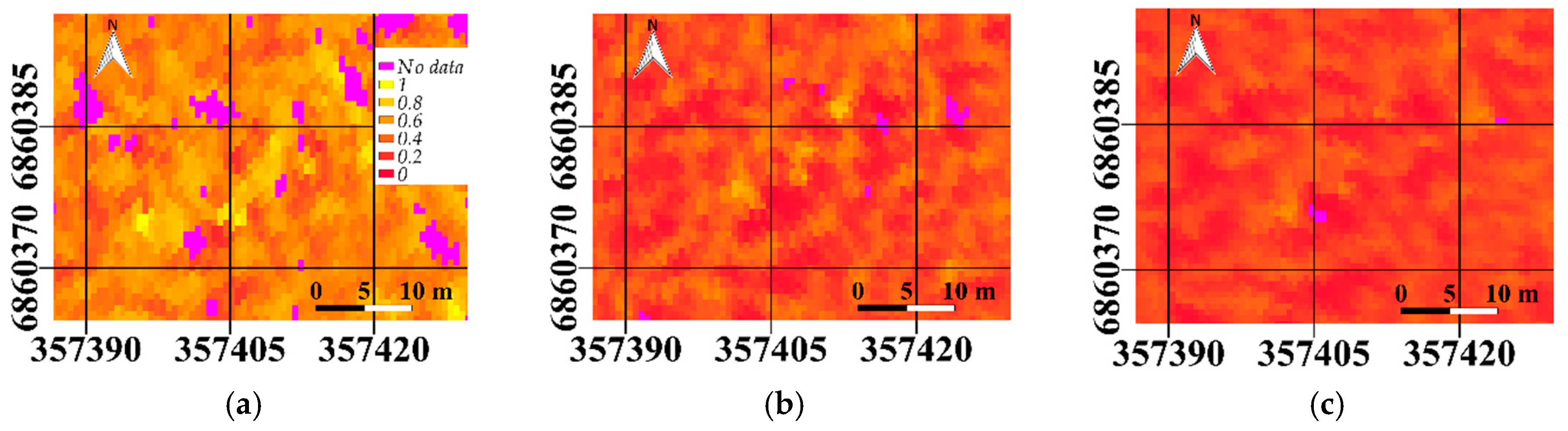
Figure 7.
Average Scots pine canopy TOC reflectance for sunlit fraction 0.26–0.29 (a); 0.35–0.36 (b); and 0.43–0.45 (c).
Figure 7.
Average Scots pine canopy TOC reflectance for sunlit fraction 0.26–0.29 (a); 0.35–0.36 (b); and 0.43–0.45 (c).

Figure 8.
Ratio of Scots pine TOC spectral reflectance between sunlit fractions for three scatter angles (β = 19°, 55°, and 76°).
Figure 8.
Ratio of Scots pine TOC spectral reflectance between sunlit fractions for three scatter angles (β = 19°, 55°, and 76°).

Figure 9.
Spectral divergence values between sunlit fraction ranges for fixed scatter angles.

Figure 10.
Non-linear fit of PRI as a function of the sunlit fraction for 19° (a); 55° (b); 76° (c); and all data (d). Lines are least squares fits of Equation (11).
Figure 10.
Non-linear fit of PRI as a function of the sunlit fraction for 19° (a); 55° (b); 76° (c); and all data (d). Lines are least squares fits of Equation (11).
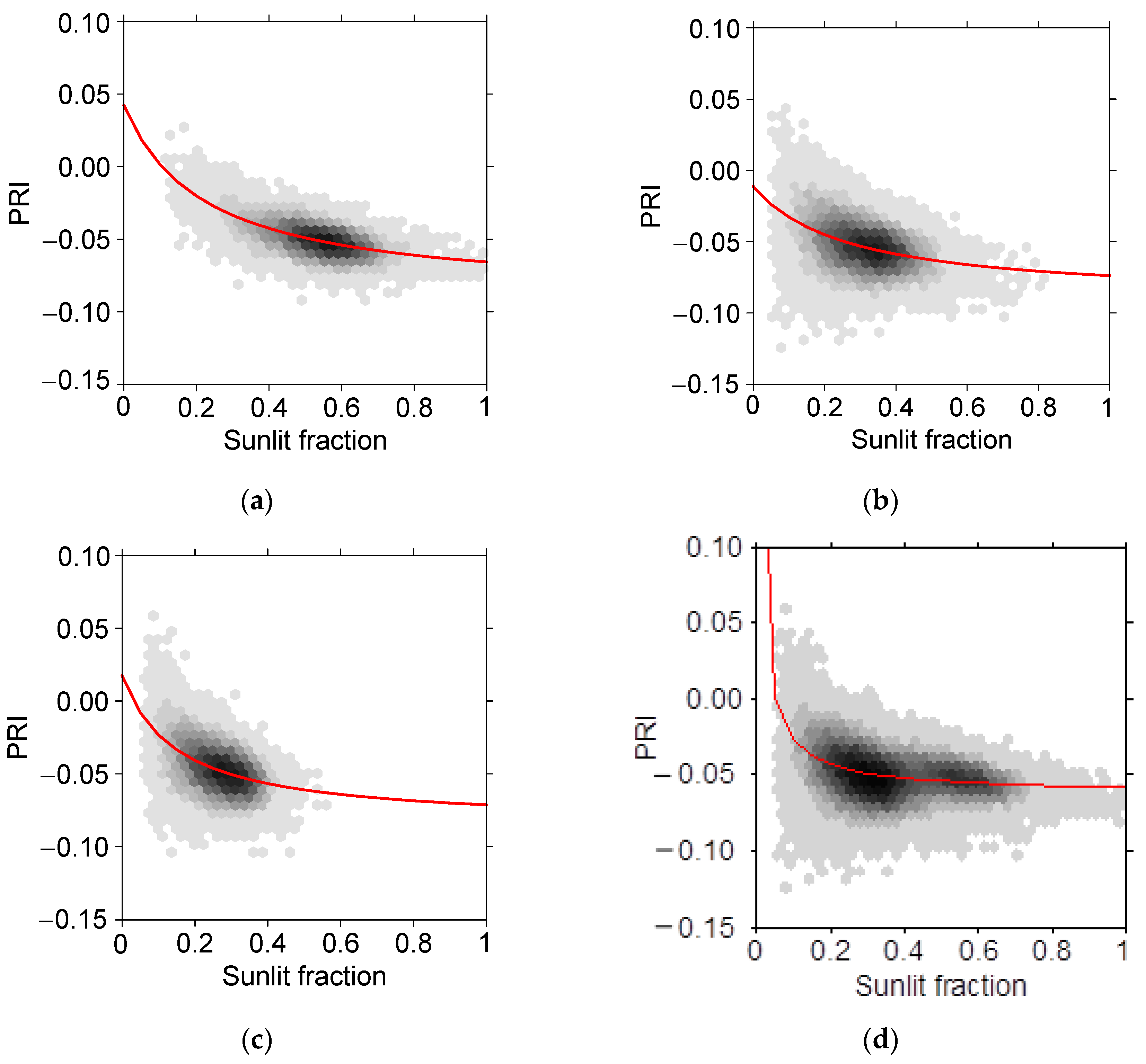
Figure 11.
Fitted PRI vs sunlit fraction curves for 19°, 55°, and 76°. Symbols denote the location of the mean sunlit fraction for each scatter angle.
Figure 11.
Fitted PRI vs sunlit fraction curves for 19°, 55°, and 76°. Symbols denote the location of the mean sunlit fraction for each scatter angle.

Figure 12.
Ratio of Scots pine canopy TOC reflectance close to hot spot () to that at dark spot () and nadir () scaled by a factor of three (for different sunlit fraction intervals, dashed lines), plotted together with the ratio of Scots pine needle reflectance to transmittance measured in situ [40] (solid line).

Table 1.
Scene and data acquisition parameters.
| l1 | l2 | l3 | |
|---|---|---|---|
| Time of acquisition (GMT+3) 03-07-2015 | 10:32 | 10:41 | 10:52 |
| Scatter angle () | 76° | 19° | 55° |
| Sensor heading (clockwise from N) | 291° | 141° | 293° |
| Solar angle (zenith, azimuth) | 48°, 122° | 48°, 125° | 47°, 128° |
| Spatial sampling interval | 0.6 × 0.7 m2 | 0.6 × 0.7 m2 | 0.6 × 0.6 m2 |
| Sensor view angle | 28° | 29° | 8° |
Table 2.
Sensor specifications and configuration during acquisitions.
| Sensor Parameter | Specification |
|---|---|
| Spectrograph | High efficiency transmissive imaging |
| Spectral range | 400–970 nm |
| Number of spectral bands | 128 |
| Spectral bandwidth | 4.7 nm |
| Framerate | 60 Hz |
| Field of view (FOV) | 37.7° |
| Across-track pixels | 1024 |
| IMU | Oxford RT3000 |
Table 3.
Number of pixels with values observed from three different viewing angles. Total number of pixels in the polygon was 35,691 for , 35,693 for , and 35,690 for .
Table 3.
Number of pixels with values observed from three different viewing angles. Total number of pixels in the polygon was 35,691 for , 35,693 for , and 35,690 for .
| Scatter Angle | Vegetated Pixels | Masked-Out Non-Vegetated Pixels |
|---|---|---|
| 19° | 33,303 | 2388 |
| 55° | 35,391 | 302 |
| 76° | 35,647 | 43 |
Table 4.
Number of pixels for seven sunlit fraction () subsets (in columns) for the three scatter angles used in the study.
Table 4.
Number of pixels for seven sunlit fraction () subsets (in columns) for the three scatter angles used in the study.
| 0.06–0.08 | 0.26–0.29 | 0.35–0.36 | 0.43–0.45 | 0.56–0.60 | 0.71–0.73 | 0.82–0.86 | |
|---|---|---|---|---|---|---|---|
| 19° | 0 | 106 | 347 | 1346 | 4837 | 413 | 86 |
| 55° | 88 | 3827 | 1327 | 1160 | 103 | 17 | 0 |
| 76° | 89 | 5411 | 1051 | 97 | 0 | 0 | 0 |
Table 5.
Scots pine canopy hemispherical-directional reflectance factor (HDRF) spectral divergence (SID) for different ranges of sunlit fraction.
Table 5.
Scots pine canopy hemispherical-directional reflectance factor (HDRF) spectral divergence (SID) for different ranges of sunlit fraction.
| 19° vs. 55° | 19° vs. 76° | 55° vs. 76° | |
|---|---|---|---|
| 0.06–0.08 | – | – | 0.001 |
| 0.26–0.29 | 0.024 | 0.037 | 0.003 |
| 0.35–0.36 | 0.022 | 0.037 | 0.003 |
| 0.43–0.45 | 0.017 | 0.033 | 0.003 |
| 0.560.60 | 0.020 | – | – |
Table 6.
Non-linear fit (Equation (11)) parameter estimates for 19°, 55°, 76° and all data combined.
Table 6.
Non-linear fit (Equation (11)) parameter estimates for 19°, 55°, 76° and all data combined.
| Parameter | 19° | 55° | 76° | Combined |
|---|---|---|---|---|
| PRI0 | 0.042 | ‒0.01 | 0.017 | 0.255 |
| Q570 | 25.6 | 20.0 | 36.6 | 549.3 |
| Q531 | 19.7 | 17.1 | 29.8 | 291.5 |
© 2017 by the authors. Licensee MDPI, Basel, Switzerland. This article is an open access article distributed under the terms and conditions of the Creative Commons Attribution (CC BY) license (http://creativecommons.org/licenses/by/4.0/).
Share and Cite
MDPI and ACS Style
Markiet, V.; Hernández-Clemente, R.; Mõttus, M. Spectral Similarity and PRI Variations for a Boreal Forest Stand Using Multi-angular Airborne Imagery. Remote Sens. 2017, 9, 1005. https://doi.org/10.3390/rs9101005
AMA Style
Markiet V, Hernández-Clemente R, Mõttus M. Spectral Similarity and PRI Variations for a Boreal Forest Stand Using Multi-angular Airborne Imagery. Remote Sensing. 2017; 9(10):1005. https://doi.org/10.3390/rs9101005
Chicago/Turabian StyleMarkiet, Vincent, Rocío Hernández-Clemente, and Matti Mõttus. 2017. "Spectral Similarity and PRI Variations for a Boreal Forest Stand Using Multi-angular Airborne Imagery" Remote Sensing 9, no. 10: 1005. https://doi.org/10.3390/rs9101005
Note that from the first issue of 2016, this journal uses article numbers instead of page numbers. See further details here.