Band Selection-Based Dimensionality Reduction for Change Detection in Multi-Temporal Hyperspectral Images


1
College of Surveying and Geoinformatics, Tongji University, Shanghai 200092, China
2
Department of Electrical and Computer Engineering, Mississippi State University, Starkville, MS 39762, USA
3
Xinjiang Institute of Ecology and Geography, CAS and the CAS Research Center for Ecology and Environment of Central Asia, Urumqi 830011, China
*
Authors to whom correspondence should be addressed.
Remote Sens. 2017, 9(10), 1008; https://doi.org/10.3390/rs9101008
Submission received: 31 August 2017
/
Revised: 23 September 2017
/
Accepted: 26 September 2017
/
Published: 29 September 2017
(This article belongs to the Section Remote Sensing Image Processing)
Abstract
:This paper proposes to use band selection-based dimensionality reduction (BS-DR) technique in addressing a challenging multi-temporal hyperspectral images change detection (HSI-CD) problem. The aim of this work is to analyze and evaluate in detail the CD performance by selecting the most informative band subset from the original high-dimensional data space. In particular, for cases where ground reference data are available or unavailable, either supervised or unsupervised CD approaches are designed. The following sub-problems in HSI-CD are investigated, including: (1) the estimated number of multi-class changes; (2) the binary CD; (3) the multiple CD; (4) the estimated optimal number of selected bands; and (5) computational efficiency. The main contribution of this paper is to provide for the first time a thorough analysis of the impacts of band selection on the HSI-CD problem, thus to fix the gap in the state-of-the-art techniques either by simply utilizing the full dimensionality of the data or exploring a complex hierarchical change analysis. It is applicable to CD problems in multispectral or PolSAR images when the feature space is expanded for discriminant feature extraction. Two real multi-temporal hyperspectral Hyperion datasets are used to validate the proposed approaches. Quantitative and qualitative experimental results demonstrated that by selecting a subset of the most informative and distinct spectral bands, the proposed approaches offered better CD performance than the state-of-the-art techniques using original full bands, without losing the change representative and discriminable capabilities of a detector.
1. Introduction
Next-generation hyperspectral sensors onboard airborne and spaceborne crafts can acquire hyperspectral images (HSIs) through dense spectral sampling (e.g., 1–10 nm) over a wide wavelength spectrum (e.g., 400–2500 nm) [1]. Hyperspectral imaging has becoming increasingly popular and important in various applications (e.g., environmental monitoring, food safety control, mineral discovery, and the military). In particular, for Earth observations, it provides materials’ spectral signatures at a fine and sophisticated level. Different from the traditional multispectral images, which characterized coarse spectral resolution in several broad spectral channels (i.e., bands), the detailed spectral sampling in hyperspectral imaging results in hundreds or even thousands of contiguous spectral bands that dramatically increases data storage volume and the ensuing data processing complexity. The high dimensionality may lead to the so-called “curse of dimensionality” or “Hughes phenomenon”, i.e., with a fixed number of training samples, the predictive power of a classifier reduces as the dimensionality increases [2,3]. Moreover, the adjacent bands are highly correlated. Such redundant information may affect how the user-interested information has been represented and detected to a great extent. The aforementioned challenges have raised many issues about handling hyperspectral data in different remote sensing tasks, e.g., classification, target detection, etc.
Dimensionality reduction (DR) techniques have been intensively investigated and used in hyperspectral image analysis [3,4,5,6,7,8,9,10,11,12,13,14,15,16]. Usually, as a kind of pre-processing method, DR techniques are able to reduce very high-dimensional data to a manageable low-dimensional space where data analysis can be performed in a more effective way [4]. By reviewing the literature, two main categories of DR methods can be summarized: transformation-based DR and band selection-based DR. The former transforms the original data into a compact feature space and analyzes the major components. Approaches such as Principle Component Analysis (PCA) [5], folded-PCA [6], Minimum Noise Fraction (MNF) [7], Independent Component Analysis (ICA) [8], Orthogonal Subspace Projection (OSP) [9], etc., have been successfully integrated into HSIs applications. The latter searches for an appropriate subset of original bands according to certain criteria and retains the physical meaning of pixels’ spectral response. In this context, Du and Yang [10] proposed an unsupervised band selection algorithm based on band similarity measurement, employing the idea from the distinctive pixel identification in endmember extraction. Yang et al. [11] designed a supervised and efficient band selection approach based on minimum estimated abundance covariance (MEAC) by using the known class signatures. Yang et al. [12] proposed a semi-supervised feature-metric-based affinity propagation (FM-AP) band selection technique, which takes advantage of the relevant component analysis to build a FM for assessing the class discrimination capability of single band and measuring the spectral correlation among bands. Patra et al. [13] developed a rough-set-based supervised band selection approach to select the informative bands having higher relevance and significant values. Jia et al. [14] developed an enhanced fast density-peak-based clustering (E-FDPC) for the unsupervised band selection task in HSI, and an isolated-point-stopping criterion was developed to automatically determine the appropriate number of bands to be selected. Yuan et al. [15] proposed a group-wise band selection framework. It evaluates the representativeness of band combination based on a multi-task sparsity pursuit criterion, where a smart yet intrinsic descriptor and a computational evolutionary strategy are used. Other new techniques such as manifold learning [16] and sparse coding [17,18] represent new trends to analyze and provide a solution to a multi-feature dataset, which have the potential to contribute to the considered BS topic in practical applications. Existing DR methods are mainly focused on solving a classification or target detection problem in a single-time HSI [3,6,10,11,12,13,14,15,16]. To the best of our knowledge, no work has been done to investigate in detail the DR technique and its impact on the multi-temporal hyperspectral images change detection (HSI-CD) task. This is very important due to the high dimensionality of hyperspectral images, and is also applicable to feature selection for CD enhancement in other types of datasets, i.e., Polarimetric Synthetic Aperture Radar (PolSAR) or multispectral images, with an increased number of expanded or extracted features.
Change detection (CD) is one of the most important remote sensing applications. Technically, it is the process identifying changes occurred between two (or more) images over a same geographical area at different observation times [19,20]. In the past decades, due to the availability of multi-temporal optical remote sensing datasets, CD tasks were intensively conducted on multispectral images [21,22,23,24,25,26,27,28]. Recently, the available multi-temporal HSIs in data archive have promoted the extension of CD research at a finer level. By considering the CD application purpose, these techniques can be mainly divided into two groups for binary CD and multiple CD [29]. Binary CD methods consider only the presence/absence of changes, without analyzing the possible different land-cover class transitions. Studies on aspects such as transformation-based CD techniques, e.g., covariance equalization and cross covariance [30,31], multivariate alteration detection (MAD) [32], Temporal-PCA (TPCA) [33], ICA [34], etc. and spectrum analysis-based CD methods, e.g., change analysis after radiometric normalization [35], target-background separation based on orthogonal subspace projection [36], etc. can be found to address the binary CD problem in HSIs. For the more challenging multiple CD, it aims to detect the changes, but also to identify different kinds of changes. Liu et al. [1] proposed a coarse-to-fine hierarchical spectral change clustering approach for detecting changes having spectral variations at different significance levels. Liu et al. [37] designed a semi-supervised sequential spectral change vector analysis (S2CVA) approach for discovering, identifying, and discriminating multiple changes according to a sequence of adaptive change projections. Liu et al. [38] investigated the spectral–temporal mixture properties in multi-temporal hyperspectral images, and proposed an unsupervised multi-temporal spectral unmixing model to address the multiple CD problem at a subpixel level. However, these works either simply utilized the full dimensionality of the feature space [30,31,32,33,35,36,38], or exploited a complex hierarchical structure of the changes [1,34,37], ignoring the potential capability of solving the HSI-CD problem in a reduced low-dimensional feature space.
In this paper, we address for the first time the challenging HSI-CD problem in a low-dimensional feature space by using band selection-based DR (BS-DR) algorithms. The most informative band subset is investigated for change representation and discrimination in an unsupervised and supervised fashion, respectively. In particular, the following issues are analyzed in detail: (1) the estimated number of changes; (2) the binary CD; (3) the multiple CD; (4) the estimated optimal number of selected bands; and (5) computational efficiency. The main contribution of this paper is, through the design of complete evaluation procedures and the obtained experimental results, to investigate the feasibility of addressing the considered high-dimensionality HSI-CD task in a reduced feature space without losing the change representative and discriminable capabilities of a detector. Note that the proposed method is also potentially applicable to practical CD applications in multi-temporal remote sensing images after having high-dimensional features, such as generated spectral, textural features, and the stacked PolSAR features derived from different coherent and incoherent decomposition models. Two multi-temporal hyperspectral Hyperion datasets are used to validate the proposed approaches. Experimental results demonstrate the effectiveness of using selected band subsets to meet or even exceed the CD performance of all original bands, and a comparable performance is observed when comparing with two state-of-the-art reference methods.
2. Methodology
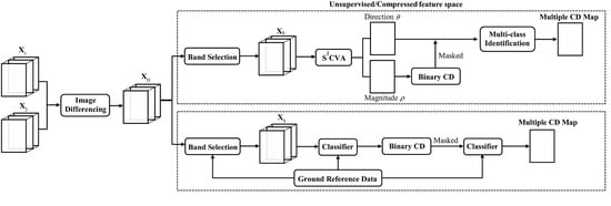
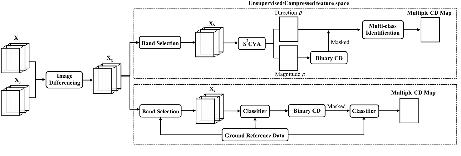
In this section, the proposed unsupervised and supervised CD approaches based on BS-DR techniques to address the considered HSI-CD problem are described in detail. The proposed approaches mainly consist of four steps: (1) full dimensional difference image construction; (2) band selection based on the difference image; (3) change feature representation; (4) change detection strategies. In particular, the unsupervised CD approach is proposed in the compressed feature space, whereas the supervised approach is based on the uncompressed features. CD performance is evaluated in detail from different perspectives following a designed evaluation procedure. Block scheme of the proposed CD approaches and the performance evaluation processes are illustrated in Figure 1. Details are given in the following subsections.
2.1. Proposed CD Approaches Based on Band Selection
2.1.1. Full Dimensional Difference Image Construction
Let X1 and X2 be two co-registered B-dimensional HSIs acquired over the same geographical area at times t1 and t2, respectively. The B-dimensional difference image XD, i.e., Spectral Change Vectors (SCVs), can be computed as:
After band selection, M-dimensional XS with M pre-defined number of bands can be extracted according to certain optimal criteria as a subset of the original B-dimensional XD. Let Ω = {ωn, Ωc} be the set of all classes in XS, where ωn is the no-change class and is the set of the K possible change classes. Therefore, the considered multiple CD problem can be formalized to detect the changed pixels (Ωc) and to identify their change classes in .
2.1.2. Band Selection Based on the Difference Image
As mentioned earlier, BS-DR approaches select a subset of the original bands to reduce data dimensionality. The intrinsic information in the original data is maintained without losing the original physical meaning of each selected channel. In this context, if prior knowledge is available as in a supervised case, band selection can be done by selecting the bands representing the most information of the user-interested targets. In an unsupervised case, the most informative and distinctive bands are selected according to certain searching criteria. In this paper we adopt an unsupervised method in [10] and a supervised method in [11] due to their excellent performance and simple implementation. Both algorithms were designed using spectral unmixing related concepts in conjunction with sequential forward search strategy. Their main steps are summarized in Table 1.
Step 1 initializes the algorithm, and readers can refer to the literature for details [10,11]. Step 2 is the key step with the employment of a proper searching criterion. A similarity criterion based on linear prediction (LP) was proposed [10], which jointly evaluated the similarity between a single band and multiple bands. Let a third band b is estimated by b1 and b2 with N pixels as:
where is the linear prediction of b, and are parameters minimizing the prediction error e, i.e., . Then a can be estimated according to the least squares solution:
where P is constructed as an N × 3 matrix, where the first column is one, and the second and third columns are the N pixels in b1 and b2, respectively. q is an N × 1 vector with all pixels in b. The band that results in the maximum error e is selected because it is the most dissimilar to b1 and b2. The algorithm can continue to select more bands.
A minimum estimated abundance covariance (MEAC) method was proposed for supervised band selection [11]. Assume that a given pixel z can be expressed according to a linear mixture model:
where S = [s1, s2, …, sp] includes the known p class spectral signatures, α is the abundance vector, and n is the uncorrelated white noise. The least squares estimation of α, denoted as , can be calculated as:
If q classes are actually present and q > p (i.e., in the situation of classes are partially known), the abundance of p classes can be estimated according to the weighted least square solution as:
The selected third band in Step 2 should let the deviation of from α be as small as possible. Hence, for the first and second case the problem is equivalent to minimizing the trace of covariance, as in [7] and [8], respectively:
where is the matrix containing signatures in selected bands Φ, and is the data covariance matrix with the selected bands in Φ only.
2.1.3. Change Feature Representation
The sequential spectral change vector analysis (S2CVA) is one of the popular state-of-the-art techniques recently proposed to solve the challenging multi-class CD problem in multi-temporal HSIs [35]. It was designed to robustly explore the hierarchical nature of complex multiple changes according to a sequential compressed feature analysis in an unsupervised fashion, without relying on the availability of ground reference data. It provides a quick yet effective solution to simultaneously address the relevant problems in CD including an estimation of the number of changes, separating the change and no-change binary information, and distinguishing different kinds of changes. In this paper, the unsupervised evaluation was mainly designed based on the S2CVA and its components.
In greater detail, S2CVA defines two change variables: change magnitude ρ and change direction θ. Magnitude ρ is the Euclidean compression of all SCVs, in which two modes can be observed on its histogram indicating the change and no-change classes. Thus the magnitude ρ is usually used for binary CD purposes. Direction θ is defined based on the spectral angle distance (SAD) [39]. It points out different types of changes with respect to the change of spectral response for a given pixel. So the multiple changes discrimination can be implemented by analyzing the direction variable θ. Mathematically, the definition of the two variables is as follows:
where and rm is the m-th (m = 1, …, M) component of XS and of an adaptive reference vector r, respectively. In particular, r is defined as the first eigenvector of eigen-decomposition of the covariance matrix A for XS [37]:
where E[XS] is the expectation of XS, W is a diagonal matrix with the eigenvalues being sorted in a descending order (i.e., ) in the diagonal, and V is the matrix of eigenvectors. The reference vector r is the first eigenvector corresponds to the largest eigenvalue λ1, which allows a projection of the considered SCVs into a reference direction that maximizes the variance of the measurement while preserving the discriminative information of different changes.
A compressed 2D polar domain [37] can be constructed based on variables ρ and θ, as shown in Figure 2. The no-change (i.e., ωn) and change (i.e., ) classes are separated along the magnitude ρ axis, and homogenous clusters present along the direction θ axis in the region indicate the possible number of multiple changes. A hierarchical analysis is originally designed in S2CVA in order to discover and detect all possible subtle changes (i.e., spectrally insignificant changes) in HSIs driven by the detection purpose at a certain level of significance. However, major changes (i.e., spectrally significant changes) can be identified at a single or several detection levels in the hierarchy. In this case, changes that are not associated with real land-cover changes (e.g., co-registration errors) can also be detected but will be defined as non-interest changes in real applications. For more details about the S2CVA technique, one can refer to [37]. Note that SCVs are projected in the defined 2D compressed polar domain, where the color of points indicates the frequency of such projections occurred in a given sector (see Figures 8 and 13).
2.1.4. Change Detection Strategies
● Proposed Unsupervised CD strategies
Based on the difference image XD, the unsupervised BS-CD algorithm [4] is applied to generate the selected band subset XS. Let the number of changes associated to the binary and multiple CD step be Kb and K, respectively. It is obvious that Kb = 2 in the binary CD to separate the Ωc and ωn two classes. The compressed magnitude of XS (i.e., ρ) (9) is analyzed, where a high pixel magnitude indicates a high probability to be changed and vice versa. It is widely used in the literature to solve the binary CD problem [1,26,37,40,41]. In this paper, two unsupervised CD algorithms, i.e., Expectation Maximization (EM) thresholding based on Bayesian decision theory [40] (denoted as Bayesian-EM) and fuzzy c-means (denoted as FCM) clustering, are considered. In particular, the EM algorithm estimates a threshold value Tρ on the magnitude ρ by searching for two modes (i.e., Ωc and ωn) on its histogram, and it is then applied to estimate automatically the class statistical parameters (i.e., prior probabilities, mean values and variances) under the framework of Bayesian decision theory [40]. The unsupervised and automatic clustering FCM algorithm is implemented by defining k = Kb = 2.
For the multiple CD, the number of changes K has to be estimated since no prior knowledge or ground reference is available. This is addressed by defining K equal to the number of homogenous change clusters present in compressed 2D polar domain in S2CVA as shown in Figure 2. Then the multiple CD is carried out on the compressed change variable θ. After masking the no-change pixels (based on the binary CD result obtained by Bayesian-EM and FCM, respectively) on the direction θ image, k-means and FCM are applied to cluster Ωc into K classes, respectively. Note that in order to reduce the uncertainty due to random initialization, the final binary CD result is provided as the average over 50 runs of k-means and FCM.
● Proposed Supervised CD strategies
For the supervised CD approaches, Kb = 2 and the number of multiple changes K is known and fixed according to the available reference map. Different from the compressed features that are used in the unsupervised approach, the supervised approach is designed based on the uncompressed M-dimensional XS. For binary CD, two-class training samples are generated from the reference map. A supervised classifier is used to classify the XS and obtain the final binary CD map. Then XS is masked, only keeping pixels belonging to Ωc according to binary CD results. The multi-class training samples are then used in the classifier to train the masked XS and generate the final multiple CD map. Two popular supervised CD methods, i.e., Support Vector Machine (SVM) [42] and Random Forest (RaF) [43] classifiers, are selected to address the multiple CD task, due to their excellent classification performance. In the SVM, the RBF kernel, and a grid-search and five-fold cross-validation are implemented to find out the optimal parameters [44]. The number of decision trees in the RaF is set as 200.
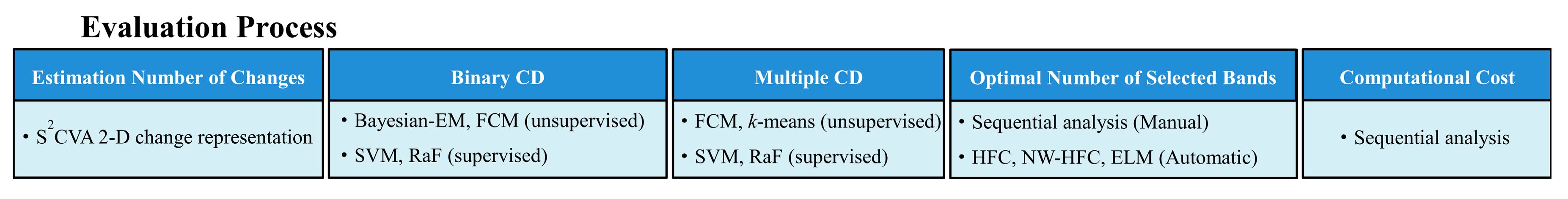
2.2 Evaluation Process
The capability and reliability of BS-DR techniques are evaluated carefully from the following five aspects in order to provide a comprehensive assessment (see Figure 3) including: (1) the estimated number of changes; (2) the binary CD; (3) the multiple CD; (4) the estimated number of selected bands; and (5) computational efficiency.
The number of multi-class changes is expected to vary in the 2D polar representation by selecting different band subsets XS. The ultimate goal is to find the XS with a given number of M that allows all K changes to be detected.
For binary and multiple CD, the overall accuracy (OA) is evaluated by comparing the binary and multiple CD results obtained by the proposed CD approaches with the known reference map. Note that for each CD approach, OA values obtained on different XS are computed by comparing with the baseline result obtained on all bands (i.e., XD). In addition, multiple CD performance was evaluated by comparing the proposed band selection-based approaches with two state-of-the-art HSI-CD techniques, i.e., hierarchical spectral change vector analysis (HSCVA) [1] and sequential spectral change vector analysis (S2CVA) [37].
In order to assess the influence of the selected band number M and find the optimal one (defined as Mopt), in this paper we analyzed Mopt from two perspectives. The first perspective is based on a sequential analysis by manually increasing the number of selected bands (i.e., M). Then the optimal parameter Mopt can be defined according to the following two strategies, which identifies the number of band subset that: (1) reaches (or exceeds) the baseline OA; and (2) results in the highest OA. The second perspective is based on the virtual dimensionality (VD) estimation approaches. Usually they are used to estimate the number of classes present in an image [10], whereas in our case they are used to make the data dimensionality high enough to accommodate all change classes for CD. Thus the estimated number can be a reference value for the number of bands to be selected. Three VD techniques are considered in this work, including the Harsanyi–Farrand–Chang (HFC) and the noise-whited HFC (NW-HFC) methods [45] and the eigenvalue likelihood maximization (ELM) approach [46], which are popular and widely used in the literature. Note that instead of implementing VD approaches on the original whole SCVs (XD) that contain both change and no-change classes, in our experiments SCVs associated with the general change class (i.e., Ωc) are considered for VD estimation, thus the estimated reference value Mopt provides potentially valuable information related to the multiple changes and their discrimination in the multiple CD task.
The computational efficiency is evaluated in the supervised SVM-based and RaF-based approaches on different XS with a certain dimensionality M. The total computational cost is the sum of cost in band-selection step and in SVM (or RaF) implementation, whereas the baseline is the computational time of SVM (or RaF) on XD. Note that due to the nature of unsupervised approaches based on two compressed features (i.e., magnitude ρ and direction θ), the time cost is only related to the band selection step itself. Therefore, they are not considered in the evaluation. Detailed analysis of time consumption has been conducted on both datasets by using Matlab R2014a, on an Intel(R) Xeon (TM) CPU E5-1630 v3 octa-core 3.70 GHz workstation with 16 GB of RAM.
3. Experimental
3.1. Dataset Descriptions
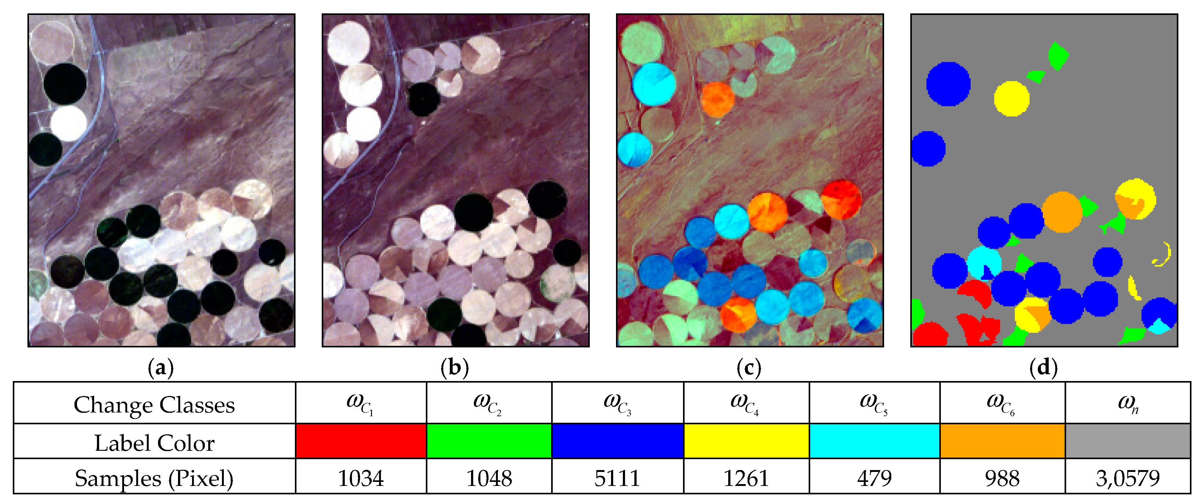
The first dataset is made up of a pair of real bitemporal hyperspectral EO-1 Hyperion remote sensing images acquired over a wetland agricultural land in Yancheng, Jiangsu Province, China. Images were acquired on 3 May 2006 (X1) and 23 April 2007 (X2), respectively. A subset of the original images is selected with a size of 220 × 430 pixels. The original Hyperion images contain 242 bands ranging from 350 to 2580 nm, characterized by a spectral resolution of 10 nm and a spatial resolution of 30 m. Pre-processing was applied on the original images including uncalibrated and noisiest bands removal, bad stripes repairing, atmospheric correction, and image co-registration, with a residual error of 0.5 pixel. Due to the fact that noisy bands with low SNR can be distinctive but not informative, they were removed in the pre-processing phase [10]. Finally, 128 pre-processed bands (i.e., 13–53, 85–96, 103–118, 135–164, 188–199, and 202–218) were used in the experiments. False color composites of X1, X2 and three bands in XD are shown in Figure 4a–c, respectively. In this scenario, five major land-cover change classes are present, mainly associated with the changes in vegetation, bare land, water, and soil. These five major changes are spectrally significant, which allows for single-level identification in the unsupervised S2CVA. Each change and no-change class and their corresponding number of samples in the reference map are provided in Figure 4. Note that the reference map was generated after careful visual analysis and image interpretation, as shown in Figure 4d. For the supervised CD approaches, class training samples are generated based on the change reference map. For binary CD, 2% of training samples were generated in each class. For multiple CD, due to the unbalanced class samples, training samples were generated as follows: 50% (class samples <1000), 2% (class samples ≥1000). Detailed class samples and their numbers are listed in Table 2.
The R2 correlation matrix was computed on the XD image as shown in Figure 5a, which represents the correlation of each spectral band with the rest of bands. So it illustrates band similarity within the considered dataset [47]. From Figure 5a, we can observe five high correlated band regions (i.e., S1: 1–25, S2: 26–41, S3: 42–53, S4: 54–69, S5: 70–128), where the adjacent bands are highly similar to each other. It indicates the necessity of implementing band selection to reduce the redundancy in those regions.
The second dataset is also made up of a pair of real bitemporal Hyperion hyperspectral images acquired on 1 May 2004 (X1) and 8 May 2007 (X2). The considered study area is an irrigated agricultural land of Umatilla County, Oregon (USA), which is a subset of the original images having a size of 180 × 225 pixels. The same preprocessing operations (i.e., uncalibrated and noisiest bands removal, bad stripes repairing, atmospheric correction, co-registration) has been done as in the previous dataset, thus finally 159 bands (i.e., 8–57, 82–119, 131–164, 182–184, and 187–220) out of the original 242 bands were used in the CD experiment. Land cover changes in this scenario mainly include the class transitions between crops, bare soil, variations in soil moisture, and water content of vegetation [36]. Figure 6a–c shows the false color composite of X1, X2, and three bands in the XD images, respectively. Note that the subtle changes associated with the road surrounding the irrigated agricultural land were not considered in this paper due to the detection needing be realized at a subpixel level [36]. Thus, in this case, six pixel-level major changes were focused. Figure 6d is the change reference map generated according to a careful image interpretation, where the six changes are shown in different colors and pixels in gray color indicate the no-change class. Detailed change and no-change class labels and their corresponding number of samples can also be found in Figure 6. Note that for binary CD, training samples were generated as 2% of each class, and for multiple CD, 10% of samples were generated for each class. Training samples used in the supervised CD are listed in Table 3.
The constructed R2 correlation matrix based on the XD image is provided in Figure 7a, where four high-correlation band regions are observed (defined as S1: 1–30, S2: 31–69, S3: 70–88, S4: 89–159). Spectral bands within these band regions are highly similar and correlated with their adjacent bands, which inevitably lead to information redundancy, thus reducing the sensitivity and accuracy of the CD process. The unsupervised LP algorithm and the supervised MEAC algorithm were applied to XD, respectively, by defining the number of bands (i.e., M) from 1 to 30. The first 20 selected bands in the two algorithms are highlighted in blue (unsupervised) and red (supervised), as illustrated in Figure 7b.
3.2. Results on the Yancheng Wetland Agricultural Dataset
The unsupervised LP algorithm and the supervised MEAC algorithm were applied to XD, while varying the selected bands (i.e., M) from 1 to 30. The first 20 selected bands in the two algorithms are highlighted in blue (unsupervised) and red (supervised) in Figure 5b. We can observe that they are located in different highly correlated spectral regions (i.e., S1–S5). This demonstrates the effectiveness of the adopted band selection approach to extract the most informative and distinctive bands, which represent information in the original data XD.
CD performance was analyzed in detail based on different selected band subsets XS with M = [1,30]. The number of multi-class changes K in the unsupervised CD is estimated according to the S2CVA 2D change representation, as described in Section 2.1.3. The estimation results are provided in Table 4. One can see that all five change classes became detectable with the minimal number of bands equal to 5. This is intuitive because K classes should be identified with at least K bands. Two S2CVA 2D scattergrams are shown in Figure 8 with M = 2 and M = 5, which allow the identification of two and five change classes, respectively (see the highlighted changes in Figure 8a,b).
For binary CD, the unsupervised Bayesian-EM, FCM approaches were applied on the compressed magnitude of XS with Kb = 2, respectively. Note that M was increased from 1 to 30 in XS. Figure 9 shows the quantitative comparison results, where we can observe that: (1) by increasing the number of selected bands M, the binary CD performance enhanced with respect to the increasing OA values. In all four approaches, OA values finally reached over the baseline; (2) two supervised approaches (i.e., SVM-based and RaF-based) resulted in higher OA values than two unsupervised ones (i.e., Bayesian-EM and FCM). In this case, the RaF-based approach achieved a similar but slightly higher performance than the SVM-based one, whereas Bayesian-EM outperformed FCM, offering higher overall OA values. A qualitative comparison of the obtained CD maps can be seen in Figure 11 row 1 and row 2. The binary CD results demonstrated that the selected informative band subsets are effective at separating changed pixels from unchanged ones.
For multiple CD, only pixels belonging to the change class (i.e., Ωc) that were obtained in the binary CD step were considered. In the unsupervised and supervised approaches, multi-class CD was conducted on the compressed 1D direction variable (XS-α) and the original B-dimensional XS, respectively. In k-means and FCM, K was equal to 5 according to the estimated number provided in Table 4. For the two supervised approaches (i.e., SVM-based and RaF-based), training samples (see Table 2) were used to train the classifiers based on the M-dimensional XS. Multiple CD results are given when M ≥ 5, which allows all five changes to be detected. Two reference approaches were also tested on this dataset. Quantitative and qualitative comparison results are shown in Figure 10 and Figure 11 (i.e., rows 3–5), respectively. One can see that the two proposed supervised approaches outperformed the unsupervised ones with respect to higher OA values. Multiple CD results showed the potential capabilities of the selected band subsets in containing sufficient information for multiple changes discrimination with a reduced dimensionality. Two reference CD methods offered similar performance to the proposed unsupervised approaches but had lower accuracy than the proposed supervised ones. Two reference methods explored the hierarchical change structure in the original full dimensionality (i.e., SCVs XD), requiring more complex change representation and discrimination.
According to the designed strategies, the selected number Mopt was analyzed manually from the multiple CD result as in Figure 10 and automatically estimated using three VD algorithms (i.e., HFC, NW-HFC, and ELM) on the masked XD with only changed pixels. Results are provided in Table 5. We can see that the estimated Mopt varies under different probability of false alarm (i.e., pf) values in HFC and NW-HFC. Three reasonable pf values are considered, producing estimates within the range of [10,15]. ELM resulted in the estimated number of Mopt equal to 13. By analyzing all obtained values in different considered approaches, we can briefly conclude that in this case, a reliable Mopt value for generating a comparable result with the baseline might be in the range of [8,13], and a higher Mopt value (e.g., [22,33]) might lead to higher CD performance.
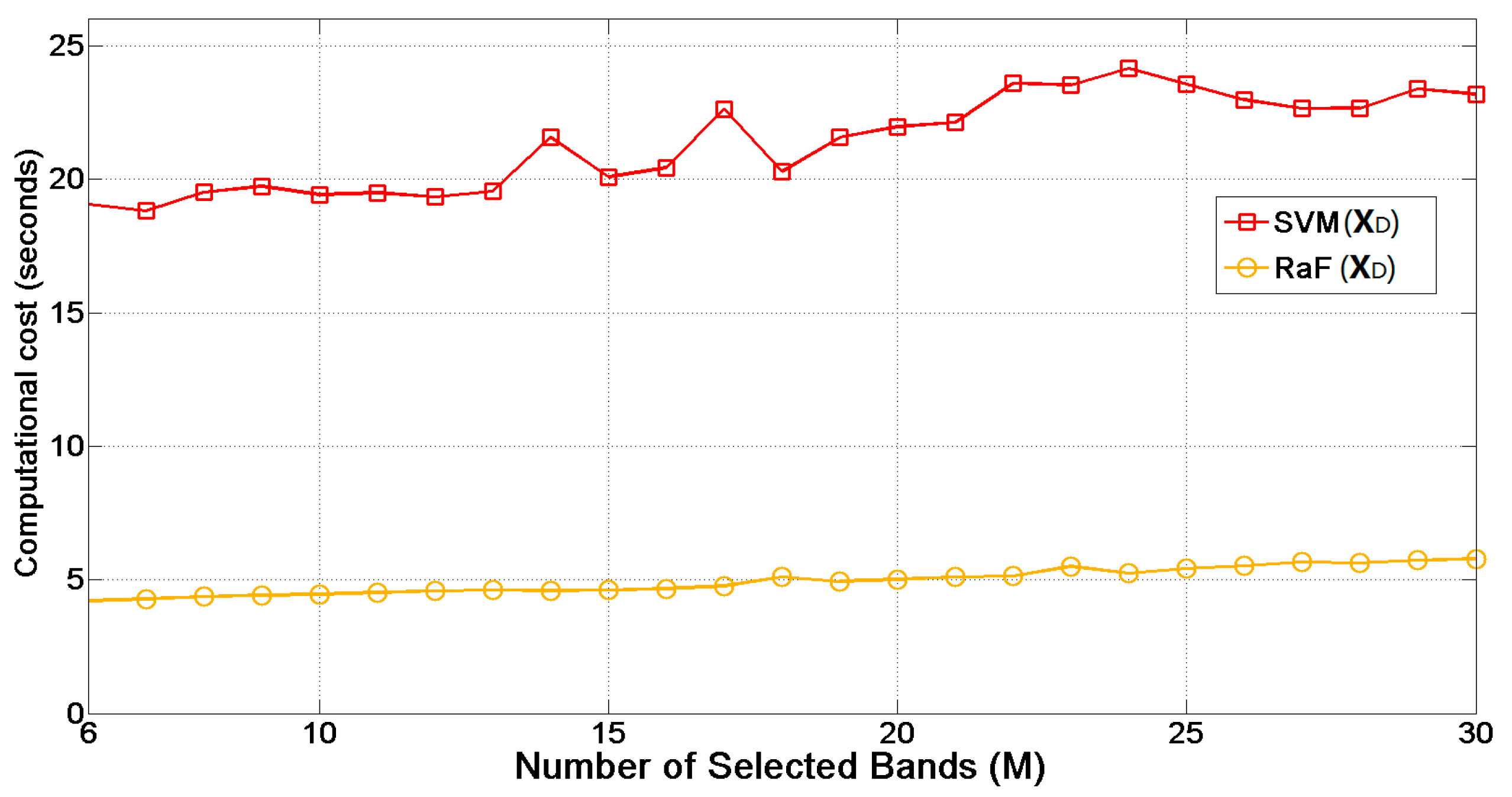
The evaluation of computational efficiency in the two proposed supervised approaches, i.e., SVM-based and RaF-based, in comparison with HSCVA and S2CVA, the two reference methods, is provided as shown in . It can be seen that by increasing the number of M in XS, the time consumed increased in both approaches, especially in the SVM-based one. The full computational time of SVM-based and RaF-based approaches obtained on XS is much lower than the baseline results based on XD. In particular, a significant reduction of time can be observed in SVM-based (i.e., from 86.23 s to an average of 35.74 s) and in RaF-based (i.e., from 15.15 s to an average of 4.87 s). Note that the computational cost of band selection for a given XS is included. RaF has more stable and efficient computational performance than SVM, which can be observed in Figure 12 and the smaller standard deviation value (i.e., 0.75). Compared with the two reference methods, the time cost of the whole procedure is much lower in the proposed approaches.
3.3. Results on the Umatilla County Irrigated Agricultural Dataset
The estimated number of multi-class changes K in the selected subset XS with M = [1,30] was obtained based on the analysis of S2CVA 2D change representation. Results are shown in Table 6. Note that in this case, the first five bands were not able to provide the correct number of all existing change classes (i.e., K = 6). Only until M = 6, all six changes became visible and detectable. This indicates that the multiple change information is implicitly represented in the first few selected bands, which is not sufficient to represent the complex changes present in the original data. Two 2D scattergrams when M = 2 and M = 6 are shown in Figure 13a,b, with the identification of four and six change classes, respectively.
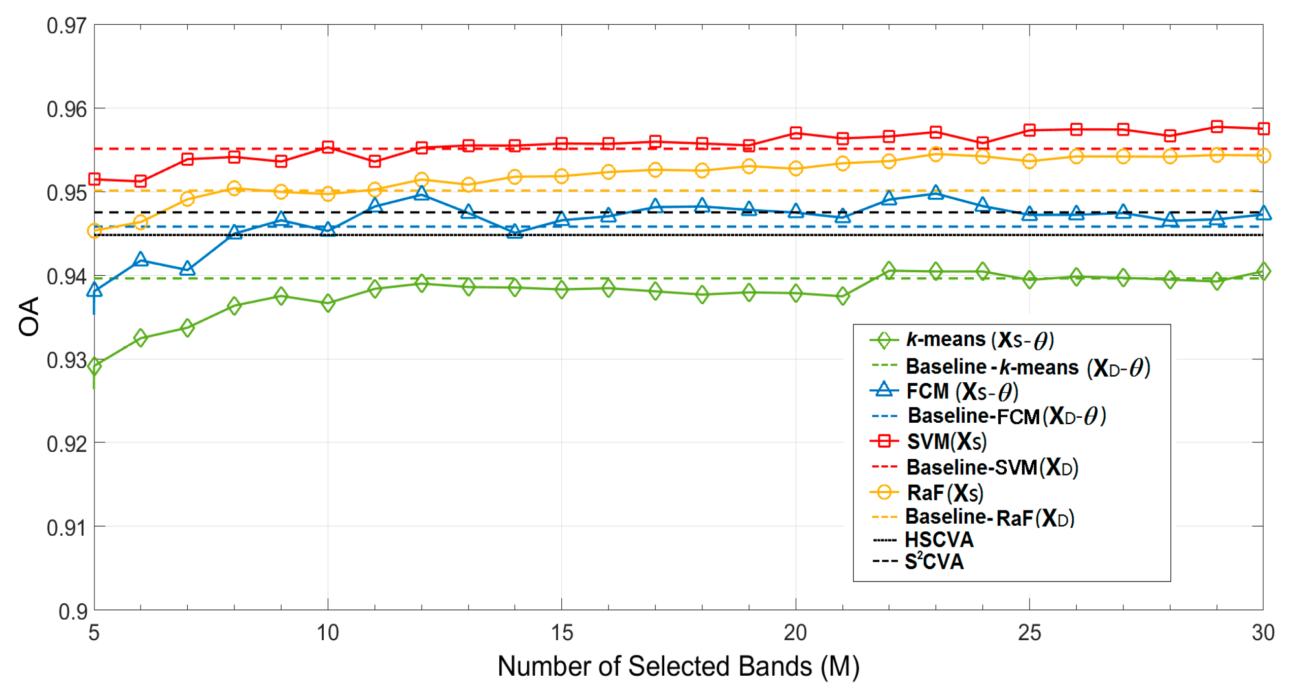
The value Kb was fixed as 2 in the unsupervised Bayesian-EM, FCM approaches for binary CD. The compressed magnitude ρ of XS was analyzed by increasing M from 1 to 30, whereas the result obtained on all bands (XD with B = 159) was considered as a baseline (illustrated as dotted lines in Figure 14). The obtained binary CD maps are shown in Figure 16 (rows 1 and 2) for qualitative comparison. Figure 14 shows the quantitative results of binary CD; one can see that by increasing the number of selected bands M, the binary CD performance improved with respect to the increasing OA values, which finally reached over the baselines and tended to be stable. This confirms that the few most informative bands are able to accomplish the binary CD task, resulting in a higher OA than when using the original full dimensionality. From the obtained OA values, SVM-based and RaF-based approaches resulted in higher OA values than the two unsupervised ones (i.e., Bayesian-EM and FCM) by taking advantage of the available training samples and supervised classifiers. In particular, the SVM-based approach had a similar but slightly better performance than the RaF-based one, whereas Bayesian-EM outperformed FCM, having higher overall OA values.
Multiple CD was carried out based on the binary CD result considering the pixels only belong to Ωc. The unsupervised k-means and FCM were applied on the compressed XS-θ variable individually, by defining k equal to the estimated number K (see Table 6). SVM-based and RaF-based approaches were implemented on the M-dimensional XS by using the multi-class training samples provided. The second dataset is also made up of a pair of real bitemporal Hyperion hyperspectral images acquired on 1 May 2004 (X1) and 8 May 2007 (X2). The considered study area is an irrigated agricultural area in Umatilla County, Oregon (USA), which is a subset of the original images having a size of 180 × 225 pixels. The same preprocessing operations (i.e., uncalibrated and noisiest bands removal, bad stripes repairing, atmospheric correction, co-registration) has been done as in the previous dataset, thus 159 bands (i.e., 8–57, 82–119, 131–164, 182–184, and 187–220) out of the original 242 bands were used in the CD experiment. Land cover changes in this scenario mainly include the class transitions between crops, bare soil, variations in soil moisture, and water content of vegetation [36]. Figure 6a–c shows the false color composite of X1, X2 and three bands in XD images, respectively. Note that the subtle changes associated with the road surrounding the irrigated agricultural land were not considered in this paper because their detection should be realized at a subpixel level [36]. Thus, in this case, six pixel-level major changes were the focus. Figure 6d is the change reference map generated according to careful image interpretation, where the six changes are shown in different colors and pixels in gray color indicate the no-change class. Detailed change and no-change class labels and their corresponding number of samples can also be found in Figure 6. Note that for binary CD, training samples were generated as 2% of each class, and for multiple CD, 10% of samples were generated for each class. The training samples used in the supervised CD are listed in Table 3.
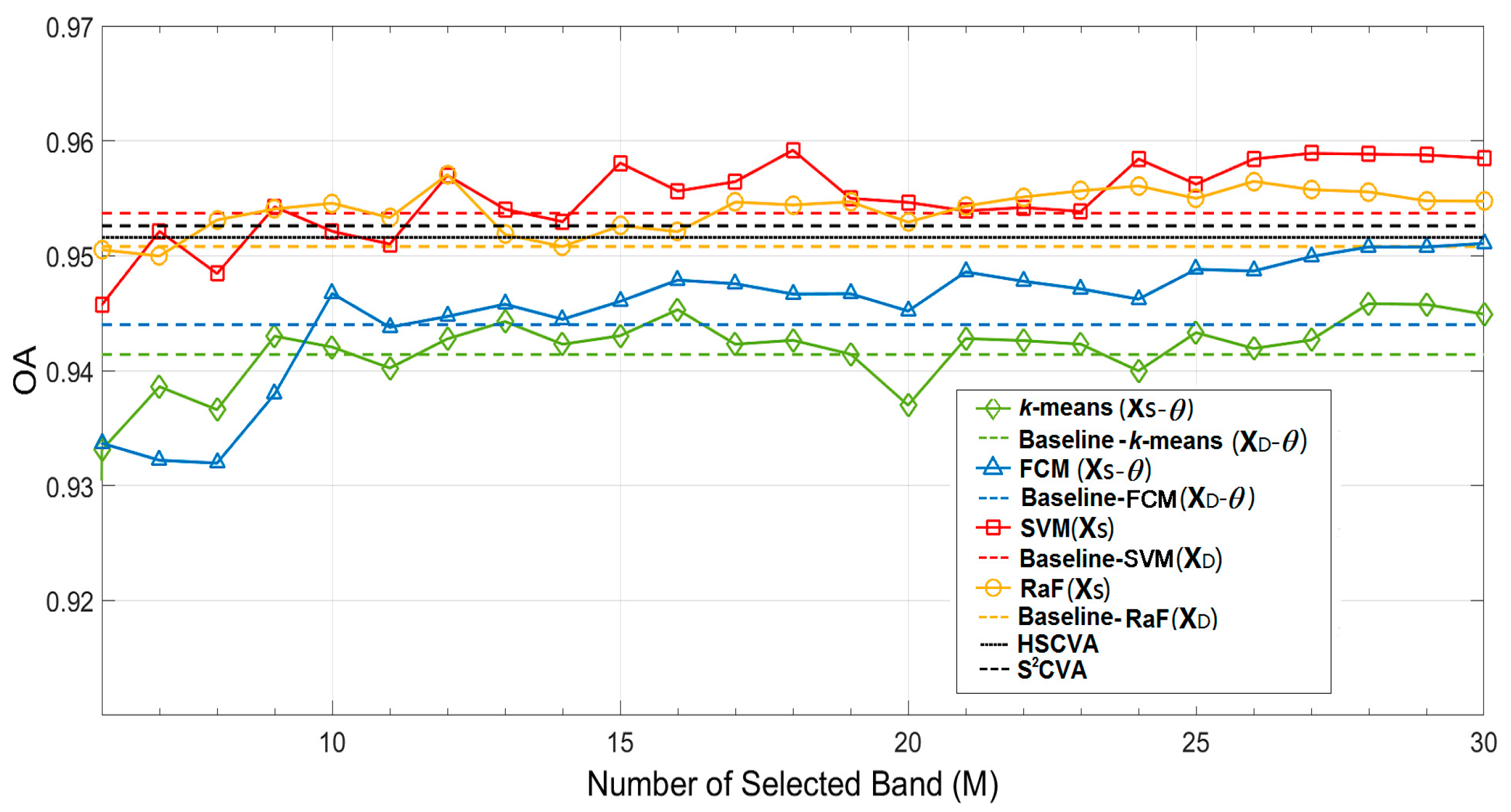
Note that results were evaluated with M ≥ 6 when all six change classes are estimated. Accuracies were also compared with those obtained by two reference methods (i.e., HSCVA and S2CVA). From the multiple CD results shown in Figure 15 and Figure 16, one can notice that by taking advantage of the supervised training process using the known reference samples and the advanced classifiers, the two proposed supervised methods resulted in better performance (higher OA values) compared with the two unsupervised ones. In particular, in this case the SVM-based approach outperformed the other three methods, having the highest OA values. The RaF-based approach had a similar but slightly lower performance than the SVM-based one. FCM showed its better discriminability in multiple CD than k-means. By increasing M, all four approaches finally exceeded the baseline results obtained using all bands (i.e., 159). This demonstrates the effectiveness of using BS-DR to enhance the change discrimination and detection performance in HSI-CD. The two hierarchical approaches yielded higher accuracies than the two unsupervised methods but lower than the supervised ones. However, full modeling of multiple changes in the original dimensionality inevitably decreases the applicability of the two reference methods.
The estimated numbers of Mopt using both manual and automatic approaches are provided in Table 7. For the automatic VD estimation approaches (i.e., HFC, NW-HFC and ELM) a reasonable pf value (e.g., 10−5, 10−4, 10−3) can be used, resulting in an estimate in the range of [9,12]. The Mopt obtained by ELM is equal to 7. By considering all the estimated Mopt values, a reliable Mopt value could be concluded within the range of [7,10], which allows the generation of comparable CD performance to the baseline. A higher Mopt value might lead to higher CD accuracy. However, a compromise should be made between the improvement of accuracy and the increase in computational cost due to the use of more selected bands.
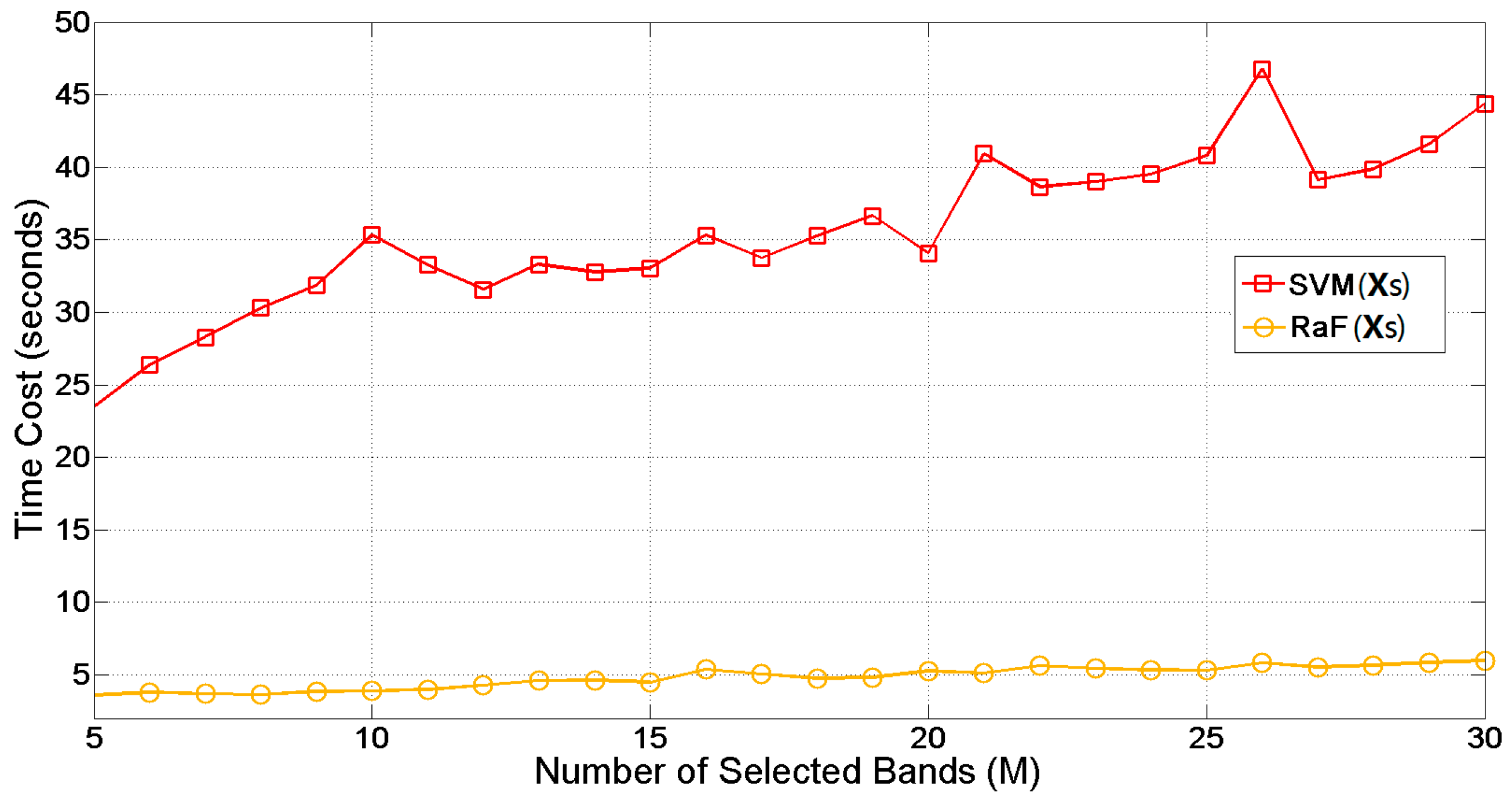
The computational efficiency of the two proposed supervised approaches, i.e., SVM-based and RaF-based, was evaluated on XS. The detailed time cost values are provided in Figure 17. It can be seen that the SVM-based approach took more time to accomplish the multiple CD task: an average of 21.42 s in the considered XS subsets, whereas the RaF-based one only took 4.95 s. The time consumed by the SVM-based approach increased with a larger number of selected bands in XS, whereas the time cost in the RaF-based one is relatively stable and low (with a lower standard deviation value equal to 0.49). Significant reduction in computational costs can be observed in SVM-based approach from the baseline cost of 68.05 s to an average of 21.42 s. The RaF-based approach is extremely fast, but the average cost (i.e., 4.95 s) is still lower than the baseline cost (i.e., 6.89 s) including both BS and CD processes. In addition, compared with the two reference approaches, a significant decrease in on the computational cost can be seen, whereas similar or even higher OA values are obtained (see Figure 15).
4. Conclusions
This paper proposes using a band selection-based DR technique to address the CD task in multi-temporal hyperspectral images. The most informative band subset with a reduced dimensionality is considered in the CD process rather than analyzing the original full dimensional data. In particular, both unsupervised and supervised band selection and CD approaches are designed by investigating the CD task from the compressed and uncompressed feature perspectives. Theoretical analysis and practical evaluation of the impact of the band selection-based DR technique on CD performance are investigated in detail with different datasets. Experimental results demonstrate that band selection can offer better CD performance when the number of selected bands is sufficiently large (e.g., 30) and can reduce the overall computational cost. Moreover, a comparable performance is obtained by comparing with two state-of-the-art HSI-CD methods using the full spectral channels.
This work contributes to fill a research gap between the state-of-the-art HSI-CD techniques simply utilizing the full high-dimensionality and the ones exploring a complex hierarchical change analysis. The considered CD task in a reduced feature space is demonstrated to be feasible without losing the change representative and discriminable capabilities of a detector. It is potentially applicable to many other CD problems with high feature dimensionality.
Acknowledgments
This work was supported by the Natural Science Foundation of China (No. 41601354, 41601440).
Author Contributions
Sicong Liu designed the proposed approaches, implemented the experiments, and drafted the manuscript. Qian Du and Xiaohua Tong revised and edited the manuscript. Alim Samat contributed the analysis tools. Haiyan Pan and Xiaolong Ma analyzed the data.
Conflicts of Interest
The authors declare no conflict of interest.
References
- Liu, S.; Bruzzone, L.; Bovolo, F.; Du, P. Hierarchical change detection in multitemporal hyperspectral images. IEEE Trans. Geosci. Remote Sens. 2015, 53, 244–260. [Google Scholar]
- Hughes, G.F. On the mean accuracy of statistical pattern recognizers. IEEE Trans. Inf. Theory 1968, 14, 55–63. [Google Scholar] [CrossRef]
- Huang, H.; Luo, F.; Liu, J.; Yang, Y. Dimensionality reduction of hyperspectral images based on sparse discriminant manifold embedding. ISPRS J. Photogramm. 2016, 106, 42–54. [Google Scholar] [CrossRef]
- Change, C.-I. Hyperspectral Data Processing: Algorithm Design and Analysis; John Wiley & Sons, Inc.: Hoboken, NJ, USA, 2013; pp. 168–198. [Google Scholar]
- Samat, A.; Du, P.; Liu, S.; Li, J.; Cheng, L. E2LMs: Ensemble extreme learning machines for hyperspectral image classification. IEEE J. Sel. Top. Appl. Earth Obs. Remote Sens. 2014, 7, 1060–1069. [Google Scholar] [CrossRef]
- Zabalza, J.; Rem, J.; Yang, M.; Zhang, Y.; Wang, J.; Marshall, S.; Han, J. Novel folded-PCA for improved feature extraction and data reduction with hyperspectral imaging and SAR in remote sensing. ISPRS J. Photogramm. 2014, 93, 112–122. [Google Scholar] [CrossRef] [Green Version]
- Du, P.; Liu, S.; Bruzzone, L.; Bovolo, F. Target-driven change detection based on data transformation and similarity measures. In Proceedings of the 2012 IEEE International Geoscience and Remote Sensing Symposium, Munich, Germany, 22–27 July 2012; pp. 2016–2019. [Google Scholar]
- Wang, J.; Chang, C.-I. Independent component analysis-based dimensionality reduction with applications in hyperspectral image analysis. IEEE Trans. Geosci. Remote Sens. 2006, 44, 1586–1600. [Google Scholar] [CrossRef]
- Harsanyi, J.C.; Chang, C.-I. Hyperspectral image classification and dimensionality reduction: An orthogonal subspace projection approach. IEEE Trans. Geosci. Remote Sens. 1994, 32, 779–785. [Google Scholar] [CrossRef]
- Du, Q.; Yang, H. Similarity-based unsupervised band selection for hyperspectral image analysis. IEEE Geosci. Remote Sens. Lett. 2008, 5, 564–568. [Google Scholar] [CrossRef]
- Yang, H.; Du, Q.; Su, H.; Sheng, Y. An efficient method for supervised hyperspectral band selection. IEEE Geosci. Remote Sens. Lett. 2011, 8, 138–142. [Google Scholar] [CrossRef]
- Yang, C.; Liu, S.; Bruzzone, L.; Guan, R. A feature-metric-based affinity propagation technique for feature selection in hyperspectralimage classification. IEEE Geosci. Remote Sens. Lett. 2013, 10, 1152–1156. [Google Scholar] [CrossRef]
- Swarnajyoti, P.; Prahlad, M.; Bruzzone, L. Hyperspectral band selection based on rough set. IEEE Trans. Geosci. Remote Sens. 2015, 53, 5495–5503. [Google Scholar]
- Jia, S.; Tang, G.; Zhu, J.; Li, Q. A novel ranking-based clustering approach for hyperspectral band selection. IEEE Trans. Geosci. Remote Sens. 2016, 54, 88–102. [Google Scholar] [CrossRef]
- Yuan, Y.; Zhu, G.; Wang, Q. Hyperspectral band selection by multitask sparsity pursuit. IEEE Trans. Geosci. Remote Sens. 2014, 53, 631–644. [Google Scholar] [CrossRef]
- Wang, Q.; Lin, J.; Yuan, Y. Salient band selection for hyperspectral image classification via manifold ranking. IEEE Trans. Neural Netw. Learn. Syst. 2017, 27, 1279–1289. [Google Scholar] [CrossRef] [PubMed]
- Liu, W.; Tao, D.; Cheng, J.; Tang, Y. Multiview Hessian discriminative sparse coding for image annotation. Comput. Vis. Image Underst. 2014, 118, 50–60. [Google Scholar] [CrossRef]
- Liu, W.; Zha, Z.; Wang, Y.; Lu, K.; Tao, D. p-Laplacian regularized sparse coding for human activity recognition. IEEE Trans. Ind. Electron. 2016, 63, 5120–5129. [Google Scholar] [CrossRef]
- Lu, D.; Mause, P.; Brondízio, E.; Moran, E. Change detection techniques. Int. J. Remote Sens. 2004, 25, 2365–2401. [Google Scholar] [CrossRef]
- Bruzzone, L.; Bovolo, F. A novel framework for the design of change-detection systems for very-high-resolution remote sensing images. Proc. IEEE 2013, 101, 609–630. [Google Scholar] [CrossRef]
- Bovolo, F.; Bruzzone, L. A theoretical framework for unsupervised change detection based on change vector analysis in the polar domain. IEEE Trans. Geosci. Remote Sens. 2007, 45, 218–236. [Google Scholar] [CrossRef]
- Bovolo, F.; Marchesi, S.; Bruzzone, L. A framework for automatic and unsupervised detection of multiple changes in multitemporal images. IEEE Trans. Geosci. Remote Sens. 2012, 50, 2196–2212. [Google Scholar] [CrossRef]
- Du, P.; Liu, S.; Gamba, P.; Tan, K.; Xia, J. Fusion of difference images for change detection over urban areas. IEEE J. Sel. Top. Appl. Earth Obs. Remote Sens. 2012, 5, 1076–1086. [Google Scholar] [CrossRef]
- Chen, X.; Chen, J.; Shi, Y.; Yamaguchi, Y. An automated approach for updating land cover maps based on integrated change detection and classification methods. ISPRS J. Photogramm. 2012, 71, 86–95. [Google Scholar] [CrossRef]
- Liu, Q.; Liu, L.; Wang, Y. Unsupervised change detection for multispectral remote sensing images using random walks. Remote Sens. 2017, 9, 438. [Google Scholar] [CrossRef]
- Chen, J.; Lu, M.; Chen, X.; Chen, J.; Chen, L. A spectral gradient difference based approach for land cover change detection. ISPRS J. Photogramm. 2013, 85, 1–12. [Google Scholar] [CrossRef]
- Tang, Y.; Zhang, L. Urban change analysis with multi-sensor multispectral imagery. Remote Sens. 2017, 9, 252. [Google Scholar] [CrossRef]
- Xiao, P.; Zhang, X.; Wang, D.; Yuan, M.; Feng, X.; Kelly, M. Change detection of built-up land: A framework of combining pixel-based detection and object-based recognition. ISPRS J. Photogramm. 2016, 119, 402–414. [Google Scholar] [CrossRef]
- Bruzzone, L.; Liu, S.; Bovolo, F.; Du, P. Change detection in multitemporal hyperspectral images. In Multitemporal Remote Sensing: Methods and Applications; Springer: Berlin, Germany, 2017; pp. 63–88. [Google Scholar]
- Schaum, A.; Stocker, A. Long-interval chronochrome target detection. In Proceedings of the 1997 International Symposium on Spectral Sensing Research (ISSSR), San Diego, CA, USA, 10–15 July 1998; pp. 1760–1770. [Google Scholar]
- Schaum, A.; Stocker, A. Hyperspectral change detection and supervised matched filtering based on covariance equalization. Proc. SPIE 2004, 5425, 77–90. [Google Scholar]
- Frank, M.; Canty, M. Unsupervised change detection for hyperspectral images. In Proceedings of the 12th JPL Airborne Earth Science Workshop, Pasadena, CA, USA, 27 February 2003; pp. 63–72. [Google Scholar]
- Ortiz-Rivera, V.; Vélez-Reyes, M.; Roysam, B. Change detection in hyperspectral imagery using temporal principal components. Proc. SPIE 2006, 6233, 623312. [Google Scholar]
- Liu, S.; Bruzzone, L.; Bovolo, F.; Du, P. Unsupervised hierarchical spectral analysis for change detection in hyperspectral images. In Proceedings of the 4th Workshop on Hyperspectral Image and Signal Processing (WHISPERS), Shanghai, China, 4–7 June 2012; pp. 1–4. [Google Scholar]
- Du, Q.; Younan, N.; King, R. Change analysis for hyperspectral imagery. In Proceedings of the International Workshop on Analysis of Multi-temporal Remote Sensing Image, Leuven, Belgium, 18–20 July 2007; pp. 1–4. [Google Scholar]
- Wu, C.; Du, B.; Zhang, L. A subspace-based change detection method for hyperspectral images. IEEE J. Sel. Top. Appl. Earth Obs. Remote Sens. 2013, 6, 815–830. [Google Scholar] [CrossRef]
- Liu, S.; Bruzzone, L.; Bovolo, F.; Zanetti, M.; Du, P. Sequential spectral change vector analysis for iteratively discovering and detecting multiple changes in hyperspectral images. IEEE Trans. Geosci. Remote Sens. 2015, 53, 4363–4378. [Google Scholar] [CrossRef]
- Liu, S.; Bruzzone, L.; Bovolo, F.; Du, P. Unsupervised multitemporal spectral unmixing for detecting multiple changes in hyperspectral images. IEEE Trans. Geosci. Remote Sens. 2016, 54, 2733–2748. [Google Scholar] [CrossRef]
- Keshava, N. Distance metrics and band selection in hyperspectral processing with applications to material identification and spectral libraries. IEEE Trans. Geosci. Remote Sens. 2004, 42, 1552–1565. [Google Scholar] [CrossRef]
- Bruzzone, L.; Prieto, D.F. Automatic analysis of the difference image for unsupervised change detection. IEEE Trans. Geosci. Remote Sens. 2000, 38, 1170–1182. [Google Scholar] [CrossRef]
- Liu, S.; Chi, M.; Zou, Y.; Samat, A.; Benediktsson, J.A.; Plaza, A. Oil spill detection via multitemporal optical remote sensing images: A change detection perspective. IEEE Geosci. Remote Sens. Lett. 2017, 14, 324–328. [Google Scholar] [CrossRef]
- Du, P.; Liu, S.; Zheng, H. Land cover change detection over mining areas based on support vector machine. J. China Univ. Min. Technol. 2012, 41, 262–267. [Google Scholar]
- Du, P.; Samat, A.; Waske, B.; Liu, S.; Li, Z. Random forest and rotation forest for fully polarized SAR image classification using polarimetric and spatial features. ISPRS J. Photogramm. 2015, 105, 38–53. [Google Scholar] [CrossRef]
- Chang, C.C.; Lin, C.J. LIBSVM: A library for support vector machines. ACM Trans. Intel. Syst. Technol. 2011, 2, 27:1–27:27. [Google Scholar] [CrossRef]
- Chang, C.; Du, Q. Estimation of number of spectrally distinct signal sources in hyperspectral imagery. IEEE Trans. Geosci. Remote Sens. 2004, 42, 608–619. [Google Scholar] [CrossRef]
- Luo, B.; Chanussot, J.; Doute, S.; Zhang, L. Empirical automatic estimation of the number of endmembers in hyperspectral images. IEEE Geosci. Remote Sens. Lett. 2013, 10, 24–28. [Google Scholar]
- Thenkabail, P.S.; Lyon, J.G.; Huete, A. Hyperspectral Remote Sensing of Vegetation; CRC Press: Boca Raton, FL, USA, 2011; pp. 93–140. [Google Scholar]
Figure 1.
Block scheme of the proposed HSI-CD approaches based on BS-DR.
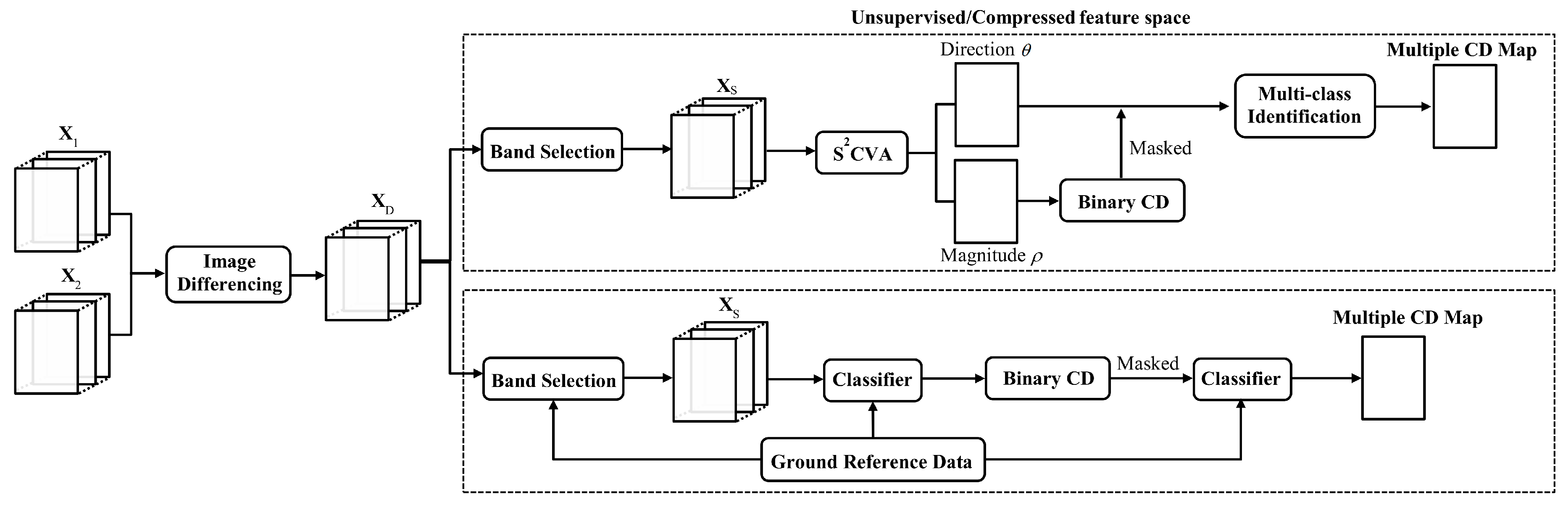
Figure 2.
The 2D compressed polar change representation in S2CVA [35].
Figure 2.
The 2D compressed polar change representation in S2CVA [35].
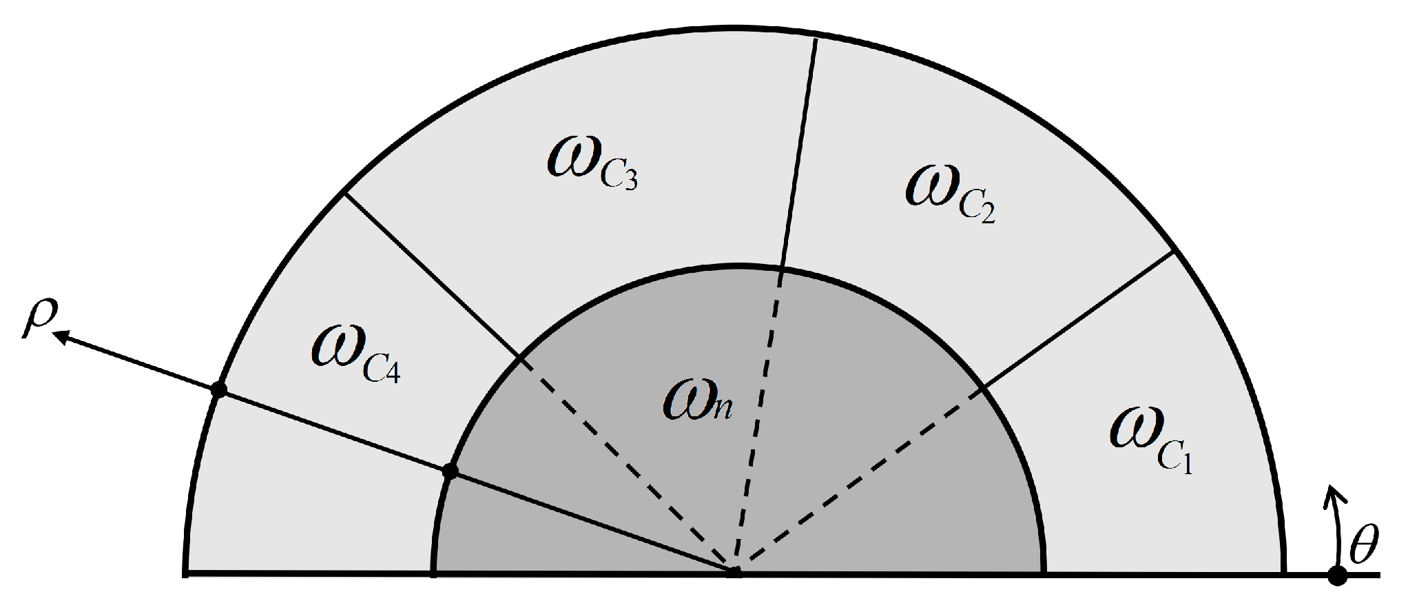
Figure 3.
Processes for evaluating the CD performance.

Figure 4.
False color composite (R: 752.4254 nm, G: 650.6727 nm, B: 548.9194 nm) of the bi-temporal EO-1 Hyperion images acquired over a wetland agricultural area in Yancheng (China) in (a) 2006 (X1) and (b) 2007 (X2); (c) composite of three SCV channels; (d) change reference map. Five changes are in different colors, whereas the unchanged pixels are in gray.
Figure 5.
(a) The R2 correlation matrix of XD image, where five highly correlated adjacent band groups are highlighted as S1–S5; (b) the first 20 selected bands and their corresponding positions in each group (Yancheng dataset).
Figure 5.
(a) The R2 correlation matrix of XD image, where five highly correlated adjacent band groups are highlighted as S1–S5; (b) the first 20 selected bands and their corresponding positions in each group (Yancheng dataset).

Figure 6.
False color composite (R: 650.67 nm, G: 548.92 nm, B: 447.17 nm) of the bi-temporal EO-1 Hyperion images acquired over an irrigated agricultural area in Umatilla County (USA) in (a) 2004 (X1) and (b) 2007 (X2); (c) composite of three SCV channels (R: 823.65 nm, G: 721.90 nm, B: 620.15 nm); (d) change reference map. Six changes are in different colors, whereas unchanged pixels are in gray.

Figure 7.
(a) The R2 correction matrix of XD image, where four highly correlated adjacent band groups are highlighted as S1–S4; (b) the first 20 selected bands and their corresponding positions in each group (Umatilla County dataset).
Figure 7.
(a) The R2 correction matrix of XD image, where four highly correlated adjacent band groups are highlighted as S1–S4; (b) the first 20 selected bands and their corresponding positions in each group (Umatilla County dataset).
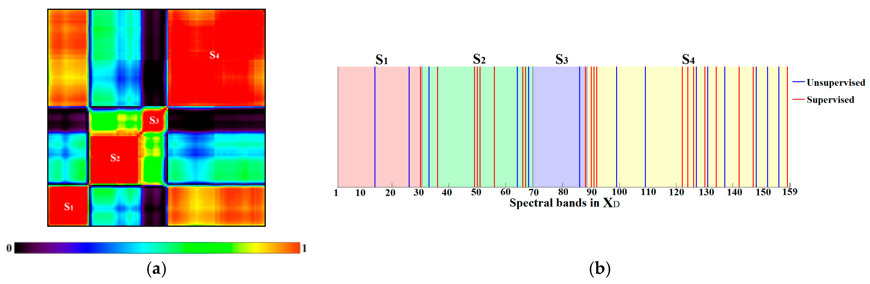
Figure 8.
S2CVA 2D change representations obtained on XS when: (a) M = 2 (two changes are identified); (b) M = 5 (five changes are identified).
Figure 8.
S2CVA 2D change representations obtained on XS when: (a) M = 2 (two changes are identified); (b) M = 5 (five changes are identified).
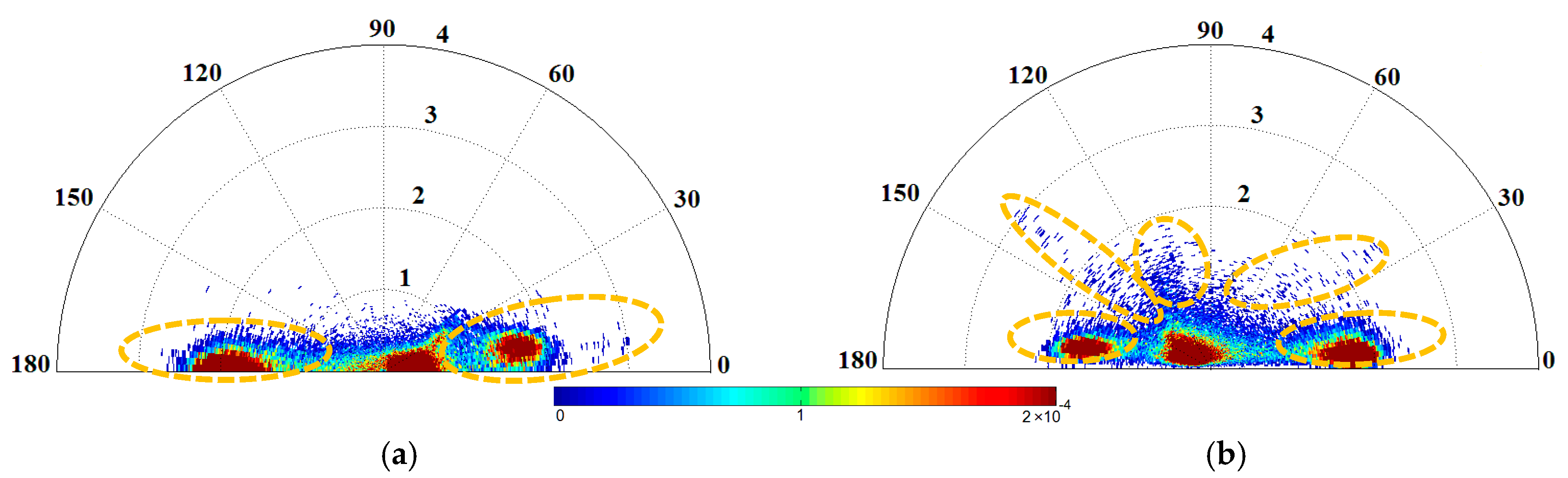
Figure 9.
Binary CD accuracies obtained by the proposed CD approaches based on BS-DR (Yancheng dataset). The unsupervised Bayesian-EM and FCM were applied on the compressed magnitude of XS (i.e., XS-ρ) and the supervised SVM-based and RaF-based approaches were applied on the uncompressed XS. Baseline results (on XD) are shown as dashed lines for comparison purposes.
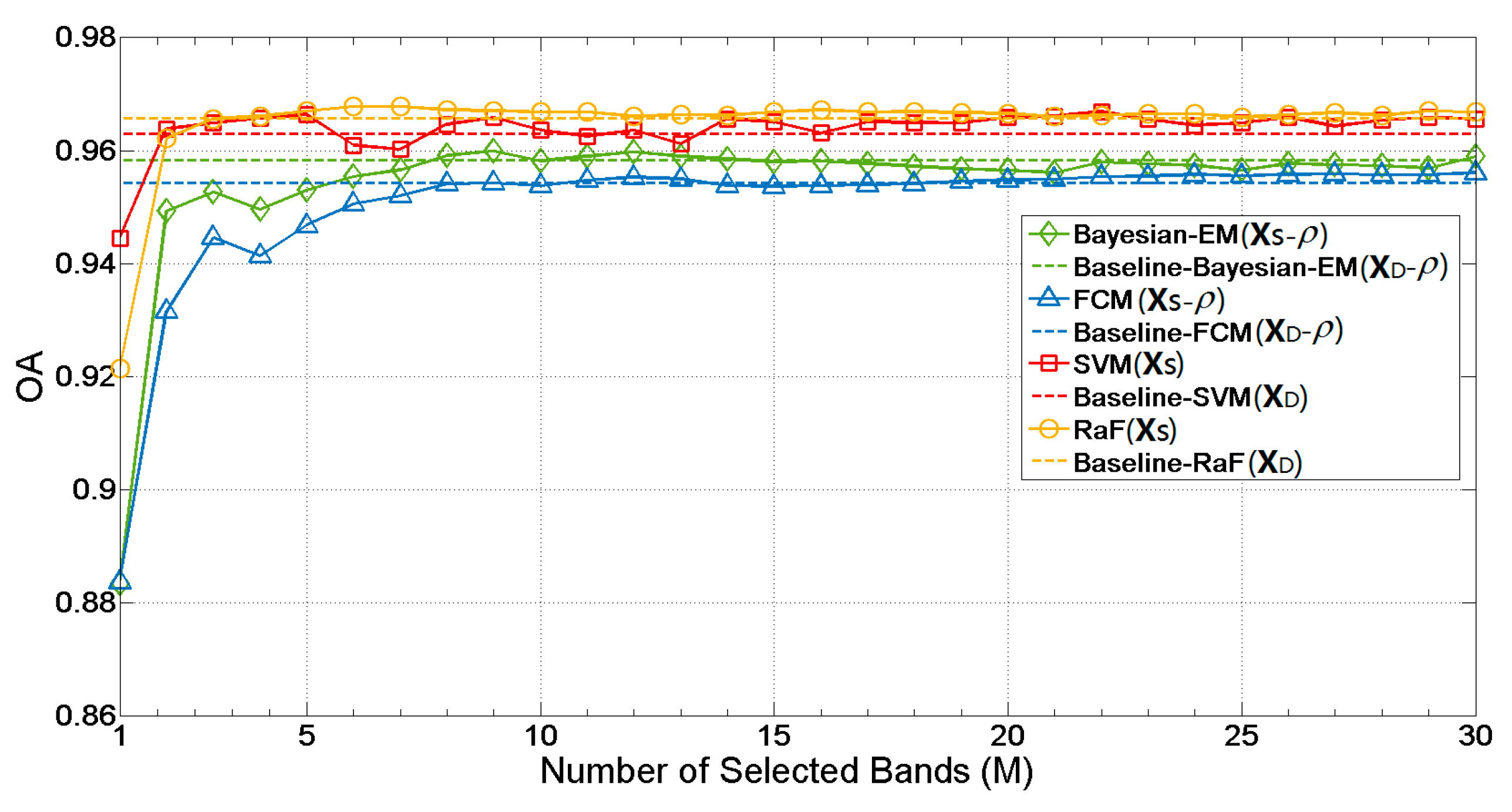
Figure 10.
Multiple CD accuracies obtained by the proposed CD approaches based on BS-DR and the reference methods (Yancheng dataset). The unsupervised k-means and FCM were applied on the compressed direction of XS (i.e., XS-θ) and the supervised SVM-based and RaF-based approaches were applied on the uncompressed XS. Baseline results on XD in the proposed approaches and in two reference methods are shown as dashed lines for comparison purposes.

Figure 11.
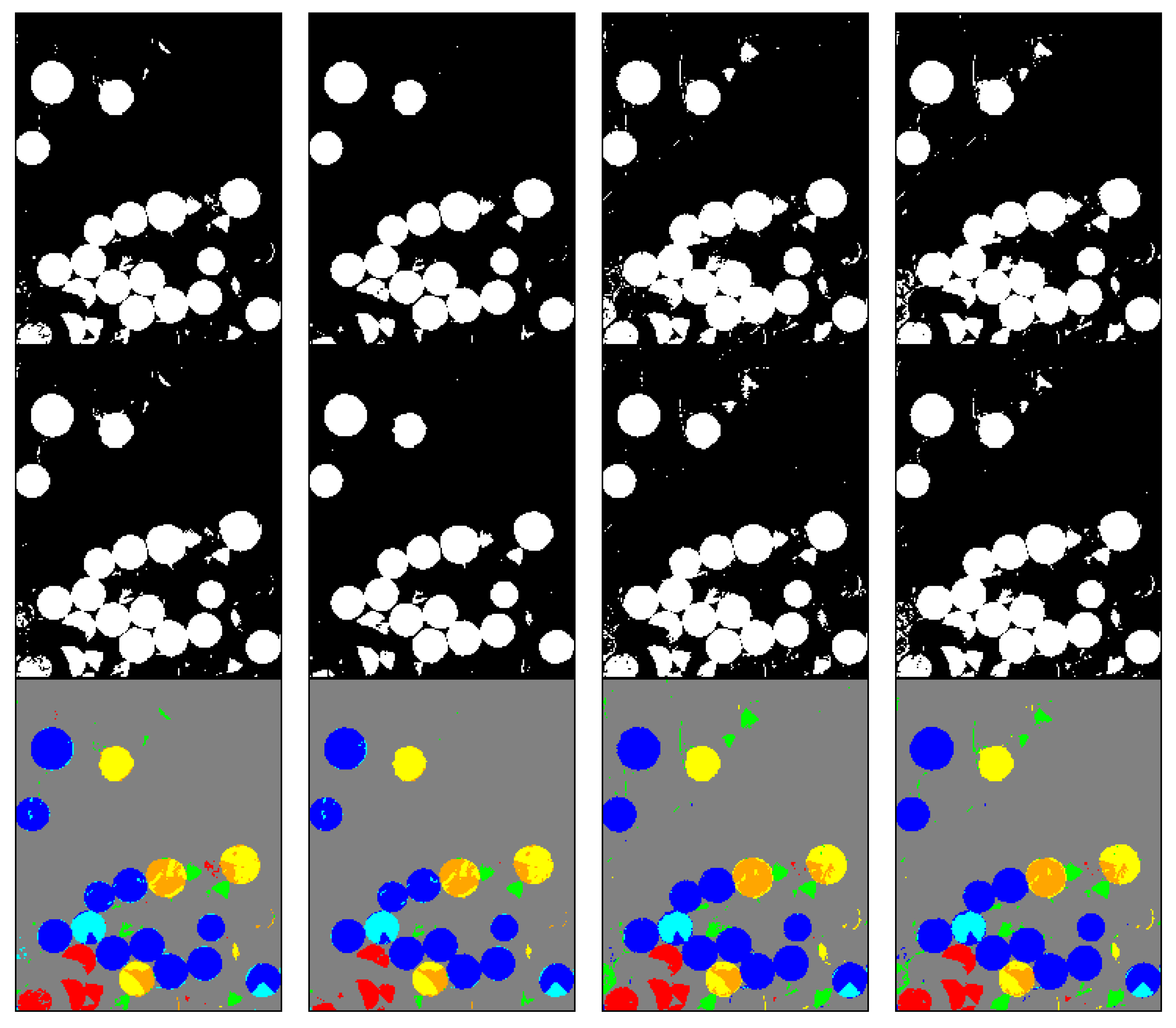
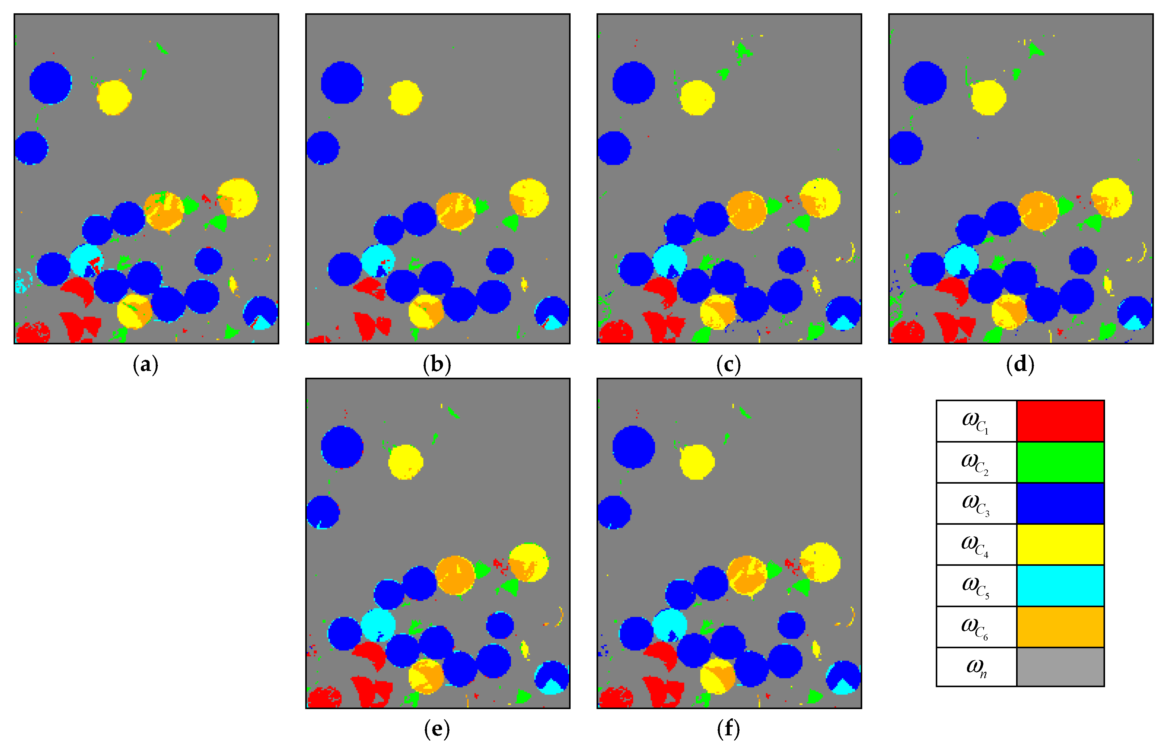
Binary (row 1–2) and multiple (row 3–5) CD maps obtained by the proposed CD approaches (Yancheng dataset). The unsupervised approaches: (a) Bayesian-EM (or k-means for multiple CD); (b) FCM. The supervised approaches: (c) SVM-based and (d) RaF-based. Rows 1 and 3 are baseline results on XD, and rows 2 and 4 are results on XS with M = 20; (e) HSCVA; (f) S2CVA.
Figure 11.
Binary (row 1–2) and multiple (row 3–5) CD maps obtained by the proposed CD approaches (Yancheng dataset). The unsupervised approaches: (a) Bayesian-EM (or k-means for multiple CD); (b) FCM. The supervised approaches: (c) SVM-based and (d) RaF-based. Rows 1 and 3 are baseline results on XD, and rows 2 and 4 are results on XS with M = 20; (e) HSCVA; (f) S2CVA.
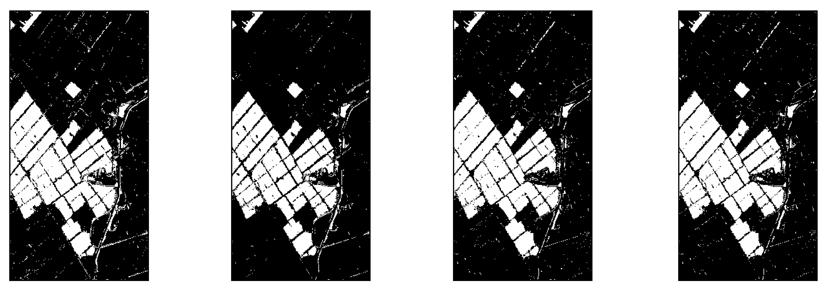

Figure 12.
Computational cost in two proposed supervised CD approaches based on different XS (mean with standard deviation), in comparison with the ones based on XD and two reference methods. Note that the time cost for band selection is included in the proposed approaches (Yancheng dataset).
Figure 12.
Computational cost in two proposed supervised CD approaches based on different XS (mean with standard deviation), in comparison with the ones based on XD and two reference methods. Note that the time cost for band selection is included in the proposed approaches (Yancheng dataset).

| Approaches | Time Cost (s) | |
|---|---|---|
| Selected XS (with M = [5,30]) | XD (Baseline) | |
| Proposed SVM-based | 35.74 ± 5.03 | 86.23 |
| Proposed RaF-based | 4.87 ± 0.75 | 15.15 |
| HSCVA | - | 103.42 |
| S2CVA | - | 79.43 |
Figure 13.
S2CVA 2D change representations obtained on XS when: (a) M = 2 (four changes were identified); (b) M = 10 (six changes were identified).
Figure 13.
S2CVA 2D change representations obtained on XS when: (a) M = 2 (four changes were identified); (b) M = 10 (six changes were identified).
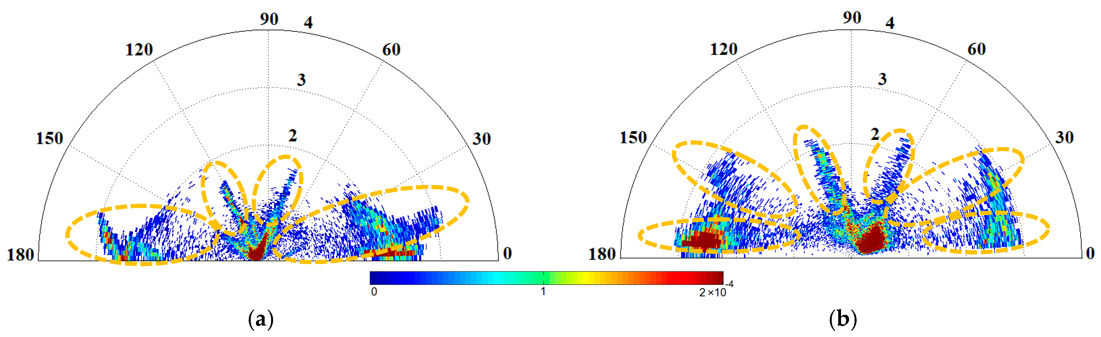
Figure 14.
Binary CD accuracies obtained by the proposed CD approaches based on BS-DR (Umatilla County dataset). The unsupervised Bayesian-EM and FCM were applied on the compressed magnitude of XS (i.e., XS-ρ) and the supervised SVM-based and RaF-based approaches were applied on the uncompressed XS. Baseline results (on XD) are shown as dashed lines for comparison purposes.

Figure 15.
Multiple CD accuracies obtained by the proposed CD approaches based on BS-DR and by the reference methods (Umatilla County dataset). The unsupervised k-means and FCM were applied on the compressed direction of XS (i.e., XS-α) and the supervised SVM-based and RaF-based were applied on the uncompressed XS. Baseline results on XD in the proposed approaches and in two reference methods are shown as dashed lines for comparison purposes.

Figure 16.
Binary (row 1–2) and multiple (row 3–5) CD maps obtained by the proposed CD approaches (Umatilla County dataset). The unsupervised approaches: (a) Bayesian-EM (or k-means for multiple CD); (b) FCM. The supervised approaches: (c) SVM-based and (d) RaF-based. Rows 1 and 3 are baseline results on XD, and rows 2 and 4 are results on XS with M = 20; (e) HSCVA; (f) S2CVA.


Figure 17.
Computational cost in two proposed supervised CD approaches based on different XS (mean with standard deviation), in comparison with the ones based on XD and two reference methods. Note that the time cost for band selection is included in the proposed approaches (Umatilla County dataset).

| Approaches | Time Cost (s) | |
|---|---|---|
| Selected XS (with M = [6,30]) | XD (Baseline) | |
| Proposed SVM-based | 21.42 ± 1.76 | 68.05 |
| Proposed RaF-based | 4.95 ± 0.49 | 6.89 |
| HSCVA | - | 89.10 |
| S2CVA | - | 56.31 |

| Main Descriptions | |
|---|---|
| Step 1 | Initialization by choosing a pair of bands to form a selected band subset Φ = {b1,b2}. |
| Step 2 | Find a third band b3 that follows a certain criterion in Φ and to update Φ = Φ ∪ {b3} |
| Step 3 | Iterate Step 2 until the number of bands in Φ reaches the convergence (reach the pre-defined number M). |
Table 2.
Number of class training samples used in the supervised CD approaches (Yancheng dataset).
| Binary CD | Multiple CD | ||
|---|---|---|---|
| Class | Training Samples (Pixels) | Change Class | Training Samples (Pixels) |
| Ωc | 483 | 170 | |
| ωn | 1409 | 290 | |
| 58 | |||
| 212 | |||
| 82 | |||
Table 3.
Number of class training samples used in the supervised CD approaches (Umatilla county dataset).
Table 3.
Number of class training samples used in the supervised CD approaches (Umatilla county dataset).
| Binary CD | Multiple CD | ||
|---|---|---|---|
| Class | Training Samples (Pixels) | Change Class | Training Samples (Pixels) |
| Ωc | 198 | 103 | |
| ωn | 612 | 105 | |
| 511 | |||
| 126 | |||
| 48 | |||
| 99 | |||
Table 4.
Estimated number of changes in multiple CD with different number of selected bands (Yancheng dataset).
Table 4.
Estimated number of changes in multiple CD with different number of selected bands (Yancheng dataset).
| Number of Selected Bands (M) | Estimated Number of Changes (K) |
|---|---|
| 1–2 | 2 |
| 3–4 | 4 |
| 5–60 | 5 |
Table 5.
Estimation of the optimal number of selected bands (Yancheng dataset).
| Approaches | Estimated Number of Mopt | ||||||
|---|---|---|---|---|---|---|---|
| Sequential Analysis (Manually) | FCM | k-means | SVM | RaF | |||
| Strategy 1 | 9 | 22 | 10 | 8 | |||
| Strategy 2 | 23 | 22 | 29 | 23 | |||
| VD Estimation (Automatic) | pf | ||||||
| 10−5 | 10−4 | 10−3 | |||||
| HFC | 12 | 13 | 14 | ||||
| NW-HFC | 10 | 12 | 15 | ||||
| ELM | 13 | ||||||
Table 6.
Estimated number of changes in multiple CD with different number of selected bands (Umatilla county dataset).
Table 6.
Estimated number of changes in multiple CD with different number of selected bands (Umatilla county dataset).
| Number of Selected Bands (M) | Estimated Number of Changes (K) |
|---|---|
| 1 | 2 |
| 2–5 | 4 |
| 6–60 | 6 |
Table 7.
Estimation of the optimal number of selected bands (Umatilla county dataset).
| Approaches | Estimated Number of Mopt | ||||||
|---|---|---|---|---|---|---|---|
| Sequential Analysis (Manually) | FCM | k-means | SVM | RaF | |||
| Strategy 1 | 10 | 9 | 9 | 9 | |||
| Strategy 2 | 30 | 28 | 18 | 12 | |||
| VD Estimation (Automatic) | pf | ||||||
| 10−5 | 10−4 | 10−3 | |||||
| HFC | 9 | 10 | 12 | ||||
| NW-HFC | 9 | 9 | 11 | ||||
| ELM | 7 | ||||||
© 2017 by the authors. Licensee MDPI, Basel, Switzerland. This article is an open access article distributed under the terms and conditions of the Creative Commons Attribution (CC BY) license (http://creativecommons.org/licenses/by/4.0/).
Share and Cite
MDPI and ACS Style
Liu, S.; Du, Q.; Tong, X.; Samat, A.; Pan, H.; Ma, X. Band Selection-Based Dimensionality Reduction for Change Detection in Multi-Temporal Hyperspectral Images. Remote Sens. 2017, 9, 1008. https://doi.org/10.3390/rs9101008
AMA Style
Liu S, Du Q, Tong X, Samat A, Pan H, Ma X. Band Selection-Based Dimensionality Reduction for Change Detection in Multi-Temporal Hyperspectral Images. Remote Sensing. 2017; 9(10):1008. https://doi.org/10.3390/rs9101008
Chicago/Turabian StyleLiu, Sicong, Qian Du, Xiaohua Tong, Alim Samat, Haiyan Pan, and Xiaolong Ma. 2017. "Band Selection-Based Dimensionality Reduction for Change Detection in Multi-Temporal Hyperspectral Images" Remote Sensing 9, no. 10: 1008. https://doi.org/10.3390/rs9101008
Note that from the first issue of 2016, this journal uses article numbers instead of page numbers. See further details here.