Comparison of Electrochemical Concentration Cell Ozonesonde and Microwave Limb Sounder Satellite Remote Sensing Ozone Profiles for the Center of the South Asian High

Abstract

To further verify the ozone profile reliability of satellite remote sensing for the ozone valley over the Tibetan Plateau in the core area of the South Asian high in summer, we validate the ozone products from the microwave limb sounder (MLS) onboard the Aura satellite over the Tibetan plateau using electrochemical concentration cell (ECC) ozonesonde data of 2016 for Ngari, Tibet. The MLS version four ozone profiles have lower standard deviation in the middle stratosphere (38–10 hPa), whereas the ozonesonde profiles have lower standard deviation in the upper troposphere and lower stratosphere region (200–83 hPa). There are statistically significant differences between these two datasets in most of the stratosphere (10–83 hPa). The mean value of MLS ozone is about 0.8–1.5 mPa greater than that of ECC ozone, which corresponds to a relative deviation of 59 ± 24% at 83 hPa, 24 ± 13% at 68 hPa, 20 ± 5% at 56 hPa, 14 ± 4% at 46 hPa and 38 hPa, and 9 ± 4% in the layers between 32 and 10 hPa. However, there is no statistically significant difference between the two datasets in the upper troposphere (100–200 hPa).

1. Introduction

The stratospheric ozone layer absorbs solar ultraviolet radiation and then heats the atmosphere. This has an important impact on the dynamical and thermodynamic structure of the stratosphere. The distribution of ozone affects the stratosphere–troposphere exchange near the tropopause and is controlled by large-scale circulation. There is a large depression in total column ozone of ~30 DU relative to the surrounding area (sometimes referred to as an ‘ozone valley’) in the upper troposphere and lower stratosphere (UTLS) region over the Tibetan Plateau [1,2,3,4,5,6], which is under the influence of the South Asian high in summer. At present, most ozone profile data are derived from satellite remote sensing instruments; for example, the Halogen Occultation Experiment (HALOE) [7], the Stratospheric Aerosol and Gas Experiment (SAGE) [8], and the microwave limb sounder (MLS) [9]. The remote-sensing algorithm used for ozone profiles shows little difference in zonal distribution, but the actual local dynamic and thermal structures vary widely, resulting in a large deviation in ozone profiles in certain locations. Therefore, it is important to compare satellite remote sensing–derived ozone profiles with ozonesonde data and correct the profiles in key areas such as the Tibetan Plateau.

Satellite remote sensing products may be validated with independent measurements. For example, the ozone products of MLS are consistent with ozonesonde data at 150–3 hPa, and the global average error is less than 8% [10]. The average deviations of the total tropospheric ozone between Global Ozone Monitoring Experiment (GOME) satellite products and ozonesonde products are within 10% [11]. Total Ozone Mapping Spectrometer (TOMS) retrieved value is lower than ground-based measurements in China [12]. MLS v4 ozone offers benefits relative to MLS v3 ozone by comparing with ozonesonde data over the Tibetan Plateau [13]. The South Asian high (Asian summer monsoon anticyclone) is a very strong circulation in the UTLS region over the Tibetan Plateau. The nearby stratospheric tracers such as ozone are greatly influenced by locations relative to South Asian high and the variation of South Asian high [1,2,3,4].

In previous studies, comparisons between ozonesonde measurements and satellite remote sensing ozone profiles for the ozone valley over the Tibetan Plateau have been mostly carried out near Lhasa, Nagqu, Kunming, and Tengchong [13,14,15,16], which are mostly located in the east of the South Asian high region (Figure 1). Ozonesonde data from the central region of the South Asian high are rare due to alpine hypoxia, bad weather, and poor traffic. However, we have obtained ozone data for summer 2016 from the balloon-borne ozonesonde at Shiquan River in Ngari, which is located in the central region of the South Asian high, providing an opportunity to validate MLS ozone version 4.2 products with ozonesonde data in this region. This study will provide a further reference for the application of satellite ozone products in the ozone valley over the Tibetan Plateau in summer.

2. Materials and Methods

2.1. Ozonesonde Data

Electrochemical concentration cell (ECC) ozonesondes are balloon-borne instruments which can make in situ measurements of ozone profile [17]. The vertical resolution of ozone is decided by ECC response time and balloon ascent rate. The typical vertical resolution is about 100–150 m [18]. ECC measurements are typically accurate to within 10% in the troposphere and 5% in the stratosphere up to 10 hPa [19]. ECC ozone sounding was performed at Shiquan River, Ngari, in Tibet (32.5° N, 80° E) for this study. The site is located in the core area of the Qiangtang Plateau, and is also close to the central region of the South Asian high. These observations are suitable for validating the ozone profiles derived from MLS satellite remote sensing data for the ozone valley over the Tibetan Plateau in summer. The detecting instrument used is the Finland Vaisala ECC ozonesonde, which is based on the relationship between ozone concentration and the intensity of the electrochemical signals generated by an electrochemical reaction between ozone and nonsaturated potassium iodide in the reaction tank [20]. The sounding balloon usually bursts by itself near an altitude of 30 km. The ECC ozonesonde measures the ozone profile during the ascent of the sounding balloon. The balloons were normally launched around midnight local time from June to September 2016. The exact dates of the 17 valid ozone profiles are 5 June, 16 June, 22 June, 25 June, 1 July, 4 July, 10 July, 13 July, 18 July, 21 July, 31 July, 25 August, 28 August, 3 September, 6 September, 12 September, and 21 September.

2.2. MLS Ozone Products

The MLS is an instrument onboard the Earth Observing System’s Aura satellite, which was launched by NASA of the United States in July 2004. The MLS measures the atmospheric composition, temperature, humidity, and cloud ice. The data quality of the MLS Level 2 Version 4 ozone products is greatly improved compared to the MLS version 3 ozone products for the UTLS region [21]. The comparisons between MLS v4 ozone and ECC ozonesonde were carried out [13,22]. The MLS v4 ozone profiles used in this study are filtered by the quality control criteria [21].

2.3. ERA-Interim Dataset

The European Center for Medium-Range Weather Forecasts interim reanalysis (ERA-Interim) global monthly dataset is used in this study [23]. The online service is at https://www.ecmwf.int/en/research/climate-reanalysis/era-interim.

2.4. Methods

To analyze the two datasets, it is first necessary to make them comparable, since they differ both in vertical resolution and the horizontal location of the ozone profiles. The MLS ozone profile nearest to the ozonesonde station in terms of horizontal distance is selected as a matching profile. The sounding time is around midnight local time, which has an offset of less than three hours relative to the nearest MLS profile in the descending orbit. Figure 1 shows the location of the matched profile on 5 June 2016 and the positions of the other 16 matching profiles. The selected profile usually has a distance within 10° longitude and 3° latitude from the ozonesonde station. The zonal distribution of stratospheric ozone is relatively uniform, so the error for this matching is small.

The vertical resolution of the MLS ozone profile is much lower than that of the ozonesonde profile. To compare the two ozone datasets at the same pressure, the ozonesonde profiles are interpolated into 16 layers of the MLS ozone between 10 and 200 hPa in log-pressure. This handling is useful for not only converting the different ozonesonde profiles to the same isobaric surface, but also comparing ozonesonde and MLS ozone profiles at the same 16 barometric layers. All the data are combined (all the days) in the figures and table. The MLS ozone unit is converted into ozone partial pressure (mPa) as that for ECC ozonesondes. Several statistical equations are used as follows:

$$\sigma =\sqrt{\frac{1}{N}{\displaystyle {\sum }_{i=1}^N{\left(x_i-\mu \right)}^2}}$$

(1)

$$b_i=\frac{{\displaystyle {\sum }_{k=1}^N\left[x_{mls}\left(k\right)-x_{sonde}\left(k\right)\right]}}{N}$$

(2)

$${\sigma }_b=\sqrt{\frac{{{\displaystyle {\sum }_{k=1}^N\left[x_{mls}\left(k\right)-x_{sonde}\left(k\right)-b_i\right]}}^2}{N\left(N-1\right)}}$$

(3)

Equation (1) is the standard deviation of a variable, also known as the mean square error or the variance of the arithmetic square root, where xi denotes the ozone value at a specific pressure, the subscript i indicates the different profiles, and μ is the average value of xi. The standard deviation can illustrate the discretization degree and the variation in an ozone dataset here. Equation (2) is the average deviation at a certain pressure between the MLS and ozonesonde data. Equation (3) is the standard error of Equation (2), which represents the distribution of the mean deviation, and it is obtained from the covariance matrix of the sample [24,25]. Equations (2) and (3) can be used to compare the difference between two ozone datasets. The difference is statistically significant when the standard error bar does not cover zero. The average deviation and the standard error can be normalized by the mean of ozonesonde data (assumed to be true value) in relative deviation analysis.

3. Results

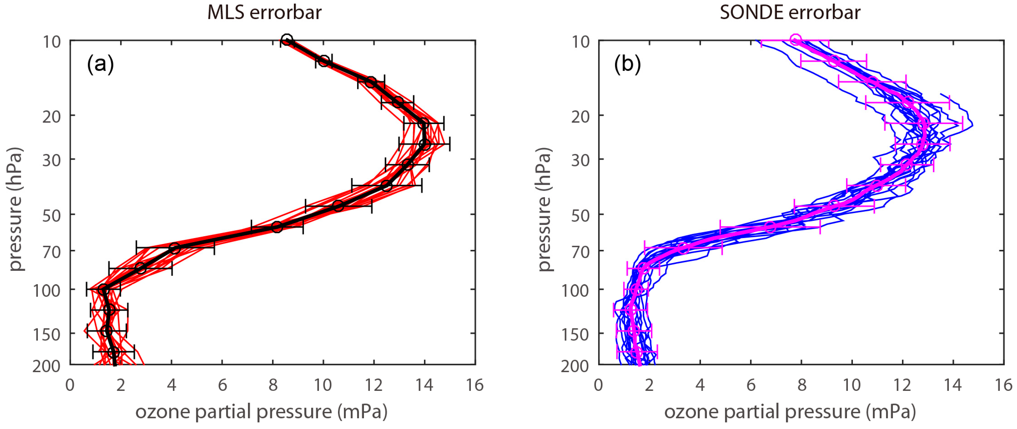
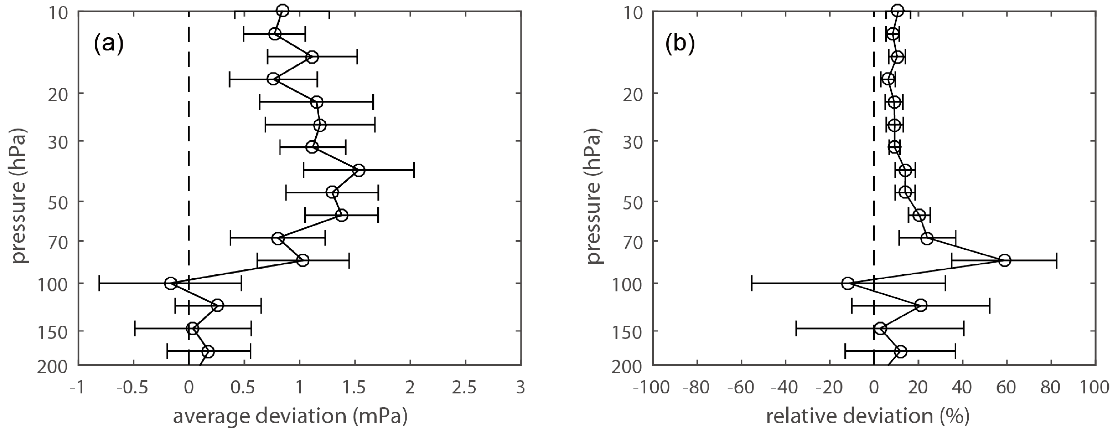
3.1. Comparison of Ozone Profiles between the Two Datasets

The two ozone datasets differ more significantly in the stratosphere than in the troposphere for the Tibetian plateau and the summer season. Figure 2 shows that a minimum ozone concentration of less than 2 mPa is located near the tropopause (about 100 to 150 hPa) in both profiles. The concentration increases with height in the stratosphere until it reaches a maximum value of greater than 12 mPa near 25 hPa, and then it decreases with height. The MLS ozone profiles have lower standard deviation in the middle stratosphere (38–10 hPa), while the ozonesonde profiles have lower standard deviation in the UTLS region (200–83 hPa).

The mean deviation of the two datasets and their reliability are shown in Figure 3. The average deviation and standard error are determined from Equations (2) and (3). At 100–200 hPa, there is no statistically significant difference between the two datasets, which is illustrated by the small average deviation (less than 0.3 mPa) with its ±2 standard error covering zero. The possible reasons are the small mean deviation of the two datasets and the large standard deviation of the MLS ozone in the UTLS region (also shown in Figure 2c). At 10–83 hPa, the standard error is smaller but the mean deviation is greater between the MLS and ozonesonde data, which illustrates that the difference is statistically significant. The ozone concentration derived from the MLS data is 0.8–1.5 mPa greater than that derived from the ozonesonde data (Figure 3a). The relative deviation of the MLS data relative to the ozonesonde data is 59 ± 24% at 83 hPa, 24 ± 13% at 68 hPa, 20 ± 5% at 56 hPa, 14 ± 4% at 46 hPa and 38 hPa, and 9 ± 4% in the layers between 32 and 10 hPa (Figure 3b). The relative deviation of MLS relative to ozonesonde over Shiquan River in the central region of the South Asian high is larger than the global MLS deviation [10] but less than that in Lhasa, Tengchong, and Naqu [13], which are located in the east of the South Asian high center.

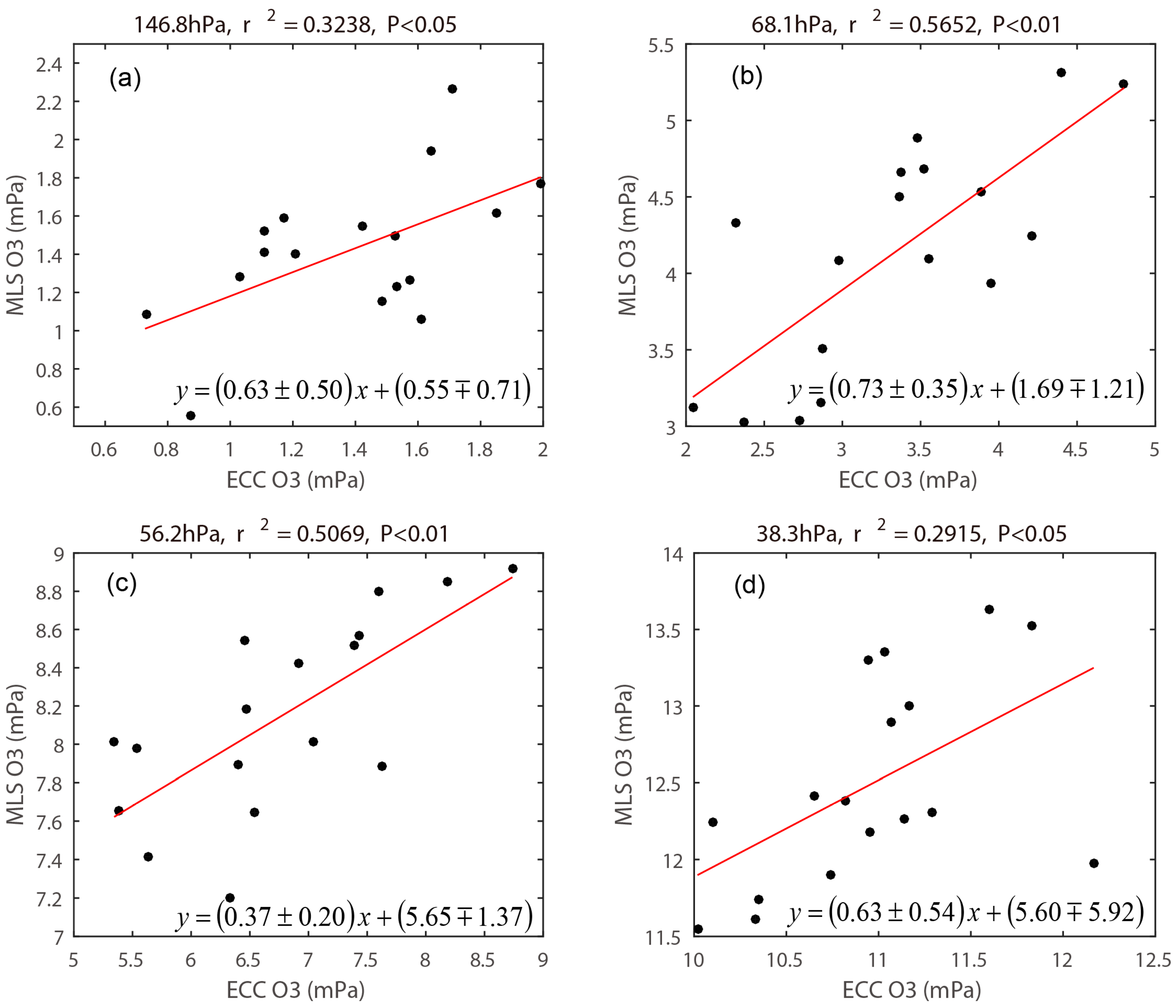
3.2. Linear Regression Analysis between MLS and Ozonesonde Data

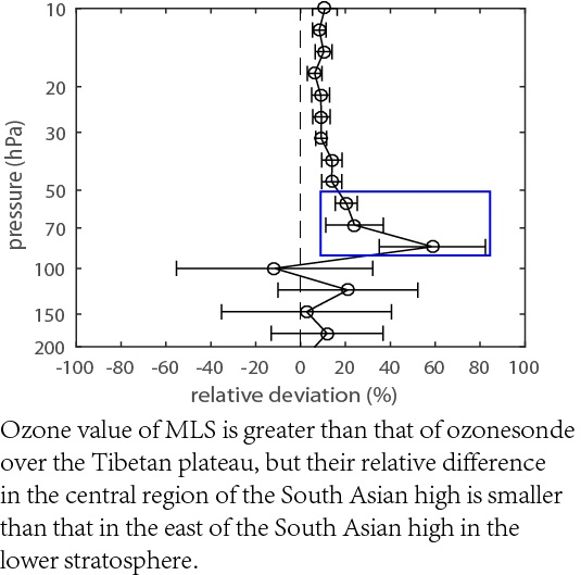
In the previous section, the data differences discussed are mainly based on the vertical distributions. The greater mean difference and smaller standard error in the stratosphere (Figure 3b) illustrate that the difference is statistically significant. As we know, MLS stratospheric ozone is more reliable than that in upper troposphere. However, the ‘true’ ECC ozonesonde data do have errors [19]. Therefore, the mean differences between the two ozone datasets could only be explained partly in the previous section. It is necessary to analyze the linear regression relationship between MLS and ozonesonde data in different layers.

Table 1. Linear regression coefficients of MLS ozone and ozonesonde.

Pressure (hPa)	Coefficient of Determination (r2)	Slope (β)	Intercept (α)	α/${\overline{\mathit{O}}}_{3\mathit{s}\mathit{o}\mathit{n}\mathit{d}\mathit{e}}$ (%)	${\overline{\mathit{O}}}_{3\mathit{s}\mathit{o}\mathit{n}\mathit{d}\mathit{e}}$ (mPa)	Probability (p)
215.4	0.03	0.43	1.04	61	1.7128	0.5186
177.8	0.01	0.05	1.61	106	1.5120	0.8391
146.8	0.32	0.63	0.55	40	1.3869	0.0171
121.2	0.10	0.34	1.08	87	1.2475	0.2285
100.0	0.01	-0.09	1.44	98	1.4687	0.7923
82.5	0.14	0.72	1.52	87	1.7561	0.1333
68.1	0.57	0.73	1.69	51	3.3368	0.0005
56.2	0.51	0.37	5.65	83	6.7669	0.0013
46.4	0.16	0.32	7.58	82	9.2981	0.1102
38.3	0.29	0.63	5.60	51	10.9522	0.0253
31.6	0.10	0.27	10.06	83	12.1725	0.2070
26.1	0.01	-0.10	15.21	119	12.7878	0.6855
21.5	0.01	0.04	13.48	105	12.8315	0.7674
17.8	0.04	0.08	12.04	99	12.1934	0.4673
14.7	0.04	0.08	11.05	102	10.8000	0.5173
12.1	0.01	-0.01	10.05	108	9.2744	0.9840

shows the linear fitting coefficients for the two ozone datasets at different pressure layers. For linear regression, ECC ozonesonde is an independent variable (we assume the ECC ozonesonde data represent true value here) and MLS ozone is a dependent variable. The slope β represents the regression coefficient and α is the intercept (which reflects the system deviation of the MLS data). There are four pressure levels (marked with shaded background) where the regression passes the significance test at the 0.05 level (using Student’s t-test). The linear regression diagrams for these four pressure levels are shown in Figure 4. The regression equation is $O_{3MLS}=\left(0.63\pm 0.50\right)\times O_{3sonde}+\left(0.55\mp 0.71\right)$ in the upper troposphere (147 hPa). In the lower and middle stratosphere (68, 56, and 38 hPa), the regression equations are $O_{3MLS}=\left(0.73\pm 0.35\right)\times O_{3sonde}+\left(1.69\mp 1.21\right)$, $O_{3MLS}=\left(0.37\pm 0.20\right)\times O_{3sonde}+\left(5.65\mp 1.37\right)$ and $O_{3MLS}=\left(0.63\pm 0.54\right)\times O_{3sonde}+\left(5.60\mp 5.92\right)$, respectively. The relative intercept of α/${\overline{O}}_{3sonde}$ at 147, 68, 56, and 38 hPa is 40 ± 51%, 51 ± 36%, 83 ± 20%, 51 ± 54%, respectively. In the upper troposphere, the regressions for most layers do not pass the significance test, mainly due to the large dispersion of the MLS data. Above 30 hPa, the regression correlation between the two datasets is not statistically significant; mainly due to the fact that the ozonesonde data has the largest standard deviation in Figure 2b. However, in the lower and middle stratosphere, the regression equations at the other two pressure levels of 83 and 46 hPa pass the significance test at the 0.15 level. Therefore, in most of the lower and middle stratosphere, the slopes are slightly less compared with the three stations in the east of the South Asian high [14], while the relative intercepts of α/${\overline{O}}_{3sonde}$ are generally greater, indicating a larger system deviation of MLS data at Shiquan River in the center of the South Asian high.

4. Discussion

Previous studies have shown that the global average difference between MLS ozone and ozonesonde data is less than 8% in most parts of the stratosphere [10]. However, the relative deviation of the MLS ozone over the Tibetan plateau is larger in this study. Nevertheless, in the lower stratosphere (especially at 83, 68, and 56 hPa), the relative difference between MLS ozone and ozonesonde over Shiquan River in the central region of the South Asian high is less than that [13] over Lhasa, Tengchong, and Naqu, which are located in the east of the South Asian high center. That may be attributed to the steady situations in the central region and the mutable conditions in the east location during the east–west oscillation (eastward–westward migration) of the Asian Summer Monsoon Anticyclone (the South Asian high) [26]. According to the linear regression relationship between MLS and ozonesonde data, in most of the lower and middle stratosphere, the slopes are slightly less compared with the three stations in the east of the South Asian high [14], while the relative intercepts of α/${\overline{O}}_{3sonde}$ are generally greater, which also indicates a larger system deviation of MLS at Shiquan River in the center of the South Asian high.

The possible reasons for this result are as follows: (1) The ozonesonde station is located in the center of the summer South Asian high, where the ozone valley is deeper than that in the surrounding area. (2) The ozonesonde samples in this study are not sufficient and the conclusions may not be universal. (3) There are some limitations and errors associated with the spatial and temporal matching between the two datasets.

5. Conclusions

The present study validates Aura MLS version 4.2 ozone products using ECC ozonesonde observations over Shiquan River, Ngari in the center of the South Asian high region in summer of 2016. The MLS ozone profiles have lower standard deviation in the middle stratosphere (38 to 10 hPa), while the ozonesonde profiles have lower standard deviation in the UTLS region (200–83 hPa). There are statistically significant differences between the two datasets in most of the stratosphere (10–83 hPa). The mean value of the MLS ozone is about 0.8–1.5 mPa greater than that of ECC ozone, which corresponds to a relative deviation of 59 ± 24% at 83 hPa, 24 ± 13% at 68 hPa, 20 ± 5% at 56 hPa, 14 ± 4% at 46 hPa and 38 hPa, and 9 ± 4% in the layers between 32 and 10hPa. However, there is no statistically significant difference between these two datasets in the upper troposphere (100–200 hPa).

References

1. Bian, J.C.; Yan, R.C.; Chen, H.B.; Lu, D.R.; Massie, S.T. Formation of the summertime ozone valley over the Tibetan Plateau: The Asian summer monsoon and air column variations. Adv. Atmos. Sci. 2011, 28, 1318–1325. [Google Scholar] [CrossRef]
2. Guo, D.; Wang, P.X.; Zhou, X.J.; Liu, Y.; Li, W.L. The dynamic effects of the South Asian high on the ozone valley over the Tibetan Plateau. Acta Meteorol. Sin. 2012, 26, 216–228. [Google Scholar] [CrossRef]
3. Guo, D.; Su, Y.C.; Shi, C.H.; Xu, J.J.; Alfred, M.P., Jr. Double Core of Ozone Valley over the Tibetan Plateau and its Possible Mechanisms. J. Atmos. Terr. Phys. 2015, 130–131, 127–131. [Google Scholar] [CrossRef]
4. Guo, D.; Su, Y.C.; Zhou, X.J.; Xu, J.J.; Shi, C.H.; Liu, Y.; Li, W.L.; Li, Z.K. Evaluation of Trend Uncertainty of Summer Ozone Valley over Tibetan Plateau in Three Reanalysis Datasets. J. Meteorol. Res. 2017, 31, 431–437. [Google Scholar] [CrossRef]
5. Li, Z.K.; Qin, H.; Guo, D.; Zhou, S.W.; Huang, Y.; Su, Y.C.; Wang, L.W.; Sun, Y. Impact of Ozone Valley over the Tibetan on South Asian High in CAM5. Adv. Meteorol. 2017. [Google Scholar] [CrossRef]
6. Zhou, X.; Luo, C.; Li, W.L.; Shi, J.E. Variation of Total Ozone in China and Low—Value Center of Qinghai—Tibet Plateau. Sci. Bull. 1995, 40, 1396–1398. [Google Scholar]
7. Russell, J.M., III; Gordley, L.L.; Park, J.H.; Drayson, S.R.; Hesketh, W.D.; Cicerone, R.J.; Tuck, A.F.; Frederick, J.E.; Harries, J.E.; Crutzen, P.J. The Halogen Occultation Experiment. J. Geophys. Res. Atmos. 1993, 98, 10777–10797. [Google Scholar] [CrossRef]
8. Mauldin, L.E.; Zaun, N.H.; McCormick, M.P.; Guy, J.H.; Vaughn, W.R. Stratospheric Aerosol and Gas Experiment II Instrument: A Functional Description. Opt. Eng. 1985, 24, 242307. [Google Scholar] [CrossRef]
9. Waters, J.W.; Froidevaux, L.; Harwood, R.S.; Jarnot, R.F.; Pickett, H.M. The Earth observing system microwave limb sounder (EOS MLS) on the aura Satellite. IEEE Trans. Geosci. Remote. Sens. 2006, 44, 1075–1092. [Google Scholar] [CrossRef]
10. Jiang, Y.B.; Froidevaux, L.; Lambert, A.; Licesey, N.J.; Read, W.G.; Waters, J.W.; Bojkov, B.; Leblanc, T.; McDermid, I.S.; Godin-Beekmann, S.; et al. Validation of Aura Microwave Limb Sounder ozone by ozonesonde and lidar measurements. J. Geophys. Res. 2007, 112, 6033–6044. [Google Scholar] [CrossRef]
11. Cai, Z.N.; Wang, Y.; Liu, X.; Zheng, X.D.; Chance, K.; Liu, Y. Validation of GOME ozone profiles and tropospheric column ozone with ozone sonde over China. J. Appl. Meteorol. Sci. 2009, 20, 337–345. (In Chinese) [Google Scholar]
12. Pan, L.; Niu, S.J. A Comparison of Total Column Ozone Values Derived from AIRS, TOVS and TOMS. J. Remote. Sens. 2008, 12, 54–63. [Google Scholar]
13. Yan, X.L.; Wright, J.S.; Zheng, X.D.; Livesey, N.J.; Vömel, H.; Zhou, X.J. Validation of Aura MLS retrievals of temperature, water vapour and ozone in the upper troposphere and lower–middle stratosphere over the Tibetan Plateau during boreal summer. Atmos. Meas. Tech. 2016, 9, 3547–3566. [Google Scholar] [CrossRef]
14. Yan, X.L.; Zheng, X.D.; Zhou, X.J.; Vömel, H.; Song, J.Y.; Li, W.; Ma, Y.H.; Zhang, Y. Validation of Aura Microwave Limb Sounder water vapor and ozone profiles over the Tibetan Plateau and its adjacent region during boreal summer. Sci. China Earth Sci. 2015, 58, 589–603. [Google Scholar] [CrossRef]
15. Bian, J.C.; Pan, L.L.; Paulik, L.; Vömel, H.; Chen, H.B.; Lu, D. In situ water vapor and ozone measurements in Lhasa and Kunming during the Asian summer monsoon. Geophys. Res. Lett. 2012, 39, L19808. [Google Scholar] [CrossRef]
16. Zhen, X.D.; Tang, J.; Li, W.L.; Zhou, X.J.; Shi, G.Y. Observational study on total ozone amout and its vertical profile over lhasa in the summer of 1998. Q. J. Appl. Meteorol. 2000, 11, 173–179. (In Chinese) [Google Scholar]
17. Vetter, K.J. Electrochemical Kinetics-Theoretical and Experimental Aspects; Translated by Academic Press Inc.; Originally Published as “Electrochemische Kinetik”; Springer: Heidelberg/Berlin, Germany, 1967. [Google Scholar]
18. Komhyr, W.D. Electrochemical concentration cells for gas analysis. Ann. Geophys. 1969, 25, 203–210. [Google Scholar]
19. Smit, H.G.J.; Straeter, W.; Johnson, B.J.; Oltmans, S.J.; Davies, J.; Tarasick, D.W.; Hoegger, B.; Stubi, R.; Schmidlin, F.J.; Northam, T.; et al. Assessment of the performance of ECC-ozonesondes under quasi-flight conditions in the environmental simulation chamber: Insights from the Jülich Ozone Sonde Intercomparison Experiment (JOSIE). J. Geophys. Res. 2007, 112, D19306. [Google Scholar] [CrossRef]
20. Komhyr, W.D.; Barnes, R.A.; Brothers, G.B.; Lathrop, J.A.; Opperman, D.P. Electrochemical concentration cell ozonesonde performance evaluation during STOIC 1989. J. Geophys. Res. 1995, 100, 9231–9244. [Google Scholar] [CrossRef]
21. Livesey, N.J.; Read, W.G.; Wagner, P.A.; Froidevaux, L.; Lambert, A.; Manney, G.L.; Millán-Valle, L.F.; Pumphrey, H.C.; Santee, M.L.; Schwartz, M.J.; et al. Version 4.2x Level 2 Data Quality and Description Document; version 4.2x-1.0; Tech. Rep. JPL D-33509; NASA Jet Propulsion Laboratory: Pasadena, CA, USA, 2015.
22. Witte, J.C.; Anne, M.; Thompson, A.M.; Smit, H.G.J.; Fujiwara, M.; Posny, F.; Coetzee, G.J.R.; Northam, E.T.; Johnson, B.J.; Sterling, C.W.; et al. First reprocessing of Southern Hemisphere ADditional OZonesondes (SHADOZ) profile records (1998–2015): 1. Methodology and evaluation. J. Geophys. Res. Atmos. 2017, 122, 6611–6636. [Google Scholar] [CrossRef]
23. Dee, D.P.; Uppala, S.M.; Simmons, A.J.; Berrisford, P.; Poli, P.; Kobayashi, S.; Andrae, U.; Balmaseda, M.A.; Balsamo, G.; Bauer, P.; et al. The ERA-Interim reanalysis: Configuration and performance of the data assimilation system. Q. J. R. Meteorol. Soc. 2011, 137, 553–597. [Google Scholar] [CrossRef]
24. Rodgers, C.D. Characterization and error analysis of profiles retrieved from remote sonde measurements. J. Geophys. Res. 1990, 95, 5587–5595. [Google Scholar] [CrossRef]
25. Von Clarmann, T. Validation of remotely sensed profiles of atmospheric state variables: Strategies and terminology. Atmos. Chem. Phys. 2006, 6, 4311–4320. [Google Scholar] [CrossRef]
26. Luo, J.L.; Song, J.Y.; Tian, H.Y.; Liu, L.; Liang, X.L. A Case Study of Mass Transport during the East-west Oscillation of the Asian Summer Monsoon Anticyclone. Adv. Meteorol. 2017, in press. [Google Scholar]
Figure 1. Trajectory distribution of MLS ozone profiles at 50 hPa on 5 June 2016 (red solid dots); the position of the nearest matching MLS profile (black hollow circle) to the Shiquan River ozonesonde station (black triangle); the remaining 16 matching MLS ozone profiles (blue crosses or hollow circles); the maximum matching distance (large black circle); and locations of the other ozonesonde stations (red triangles for Lhasa, Nagqu, Tengchong, and Kunming). The geopotential height (pink contours; m) in July and August 2016 is from the ERA-Interim dataset.
Remotesensing 09 01012 g001
Figure 2. (a) Ozone profiles (red) and the mean profile with ±2 standard deviation (black) derived from MLS data. (b) As in (a), but derived from ozonesonde data. (c) Mean ozone profiles with ±2 standard deviation for MLS (red) and ozonesonde (blue).
Remotesensing 09 01012 g002aRemotesensing 09 01012 g002b
Figure 3. (a) Average deviation of MLS ozone profile relative to the ozonesonde profile with ±2 standard error. (b) As in (a), but for relative deviation.
Remotesensing 09 01012 g003
Figure 4. Linear regression relationship between MLS and ozonesonde data in the different layers: (a) 146.8 hPa; (b) 68.1 hPa; (c) 56.2 hPa; (d) 38.3 hPa. The interval estimate of the regression coefficient is given according to the 5% significance level.
Remotesensing 09 01012 g004