Global Registration of 3D LiDAR Point Clouds Based on Scene Features: Application to Structured Environments

Abstract

Acquiring 3D data with LiDAR systems involves scanning multiple scenes from different points of view. In actual systems, the ICP algorithm (Iterative Closest Point) is commonly used to register the acquired point clouds together to form a unique one. However, this method faces local minima issues and often needs a coarse initial alignment to converge to the optimum. This paper develops a new method for registration adapted to indoor environments and based on structure priors of such scenes. Our method works without odometric data or physical targets. The rotation and translation of the rigid transformation are computed separately, using, respectively, the Gaussian image of the point clouds and a correlation of histograms. To evaluate our algorithm on challenging registration cases, two datasets were acquired and are available for comparison with other methods online. The evaluation of our algorithm on four datasets against six existing methods shows that the proposed method is more robust against sampling and scene complexity. Moreover, the time performances enable a real-time implementation.

Data Set: https://liris.cnrs.fr/3d-registration/

Data Set License: ODC Attribute License

1. Introduction

3D registration is the process of consistently aligning two or more sets of three-dimensional points. In many applications, these sets, also called point clouds, are acquired by 3D scanners from different viewpoints and are expressed in the sensor frame. The registration process leads to the relative pose (position and orientation) between views in the same coordinate frame, such that overlapping areas between the point clouds match as well as possible. Once aligned, the individual point clouds can be fused into a single one, so that subsequent processing steps such as object reconstruction and building inspection [1] can be applied. Point cloud registration appears as a recurring task for a number of applications ranging from computer vision, computer graphics and robotic perception to photogrammetry, cultural heritage modeling and digital archeology [2]. This process is often encountered in studies related to object modeling, tracking or Simultaneous Localization And Mapping (SLAM) [3]. Such a wide applicability motivated intense research in the past few years. A first goal has been to obtain accurate alignments for challenging 3D data such as isotropic or non-distinctive objects. Another objective was to make the registration process as automatic as possible. This study deals with the registration of 3D LiDAR scans in structured environments such as indoor scenes. In this specific context, existing algorithms lack accuracy and cannot solve the registration problem in all configurations. Most of them are time-consuming and not suited to noisy data. In the case of building reconstruction applications, physical targets are usually used to ensure correct registrations. Nevertheless, setting up these targets requires extra effort and complicates the acquisition process. Some methods have been proposed to make the registration semi-manual [4], but the automatic case remains unsolved. In the case of SLAM applications, odometry measurements are usually included in the process to improve the result. However, in order to have sufficient accuracy, one has to work with more expensive and heavier equipment.

The most popular algorithm in practical automatic pipelines is ICP (Iterative Closest Point) [5]. The ICP algorithm iteratively establishes correspondences between points of a scan called the source and points of another one called the target, filters them and minimizes the spatial distance between points in each pair. To establish the correspondences, the algorithm performs a computationally-expensive nearest neighbor search, which limits the number of points that can be processed within a reasonable time. Moreover, the iterative process makes this algorithm hard to implement in real time. As the cost function is not convex, the minimization can lead to a local minimum. To address this issue, one can provide the algorithm with scans that are initially closely aligned, either adapting the acquisition phase with less motion between scans or finding a coarse alignment beforehand. This coarse alignment can be manual, given by odometry measurements or provided by potentially expensive algorithms that do not necessarily converge.

At the present time, few methods solve the registration problem regardless of the overlap and the initial positions of the point clouds. In this study, we aim at developing a new pipeline to perform registration without using local correspondences, odometric measurements or coarse initial alignment.

The work proposed in this paper deals with geometric features of structured environments such as the parallelism of walls, ceiling and floor. We evaluated the algorithm on four datasets. Two of them were acquired at the Institut Pascal to get a reliable ground truth and different acquisition contexts. They are available at https://liris.cnrs.fr/3d-registration. Section 2 briefly describes related methods. In Section 3, the proposed method is developed. In Section 4, the experiments to evaluate the method are described. The results of the evaluation are provided in Section 5. After a discussion (Section 6), we finally conclude in Section 7.

2. Related Work

The first proposed method to register point clouds is based on the Gaussian sphere mapping [6]. It consists of the representation of the normals as points on a unit radius sphere. The main idea is to sample the Gaussian image and the rotation space represented as a sphere and evaluate the similarities between the Gaussian images transformed by the rotation samples. The difficulty lays in the sampling of the rotation space, which must be as uniform and cover as many rotations as possible. Horn implemented the Extended Gaussian Sphere (EGI) [7] to add the information of the plane surface represented on the sphere to ease the matching of points. The Complex Extended Gaussian Sphere (CEGI) [8] is another extension that allows one to successively derive the rotation using the same method as EGI and the translation between two point clouds after adding the information of the distance between the planes and the origin. These approaches require a complete overlap of the point clouds. The last improvement of the method was proposed by Makadia et al. [9]. It consists of applying a spherical correlation between the sampled Gaussian images to determine the best rotation. However, all of these methods based on sampling the transformation space only lead to a coarse alignment.

The well-known ICP algorithm outperforms the previous methods. Many works have tried to improve this algorithm’s robustness [10,11]. Some methods focus on the cost function metric. Indeed, the correspondences found between points cannot be exact because of the different sampling rates of the scans and the noise introduced by the sensors. The point-to-plane ICP [12] and generalized ICP [13] have been proposed to solve this issue. Other methods improve the minimization process to make it more robust to local minima and to speed up the optimization. In [14] for example, the Levenberg–Marquardt algorithm is used to find the optimum. In [15], a least squares method is applied. Recently, the new algorithm Go-ICP [16] was introduced to solve the non-convexity problem. It alternates between an ICP process and a process based on branch and bound to make a search in the transformation space. This algorithm has been proven to converge to the optimal solution. However, it becomes rapidly time consuming due to the repeated nearest neighbor search implied by the ICP algorithm and the search in the transformation space. In practice, it remains difficult to use with large datasets such as indoor environment scans of tens of thousands of points. Another way to improve the results of this algorithm is to preprocess the input points. In [17], a method of sampling the input data based on the covariance of the input points leads to an improvement of ICP performances. ICP-based algorithms are largely used in association with odometry measurements in SLAM pipelines because of their easy implementation and their rapidity. However, to deal with the accuracy issue, a closed loop must be included in the acquisition, and a global optimization must be performed. Borrmann et al. proposed such a pipeline for a six degree of freedom SLAM [18].

Holz et al. created a pipeline including ICP to ensure the convergence of the algorithm [19]. First, a coarse alignment is determined, and then, a refinement step such as ICP or one of its variants is performed. To derive a coarse alignment, some keypoints are selected [20], then their local descriptors are computed using their neighborhoods. The most known descriptors are Fast Point Feature Histograms (FPFH) [21], spin-images [22] and the Signature of Histograms of Orientations (SHOT) [23]. Another way to get keypoints is described in [24], where the points’ intensity information is used to create 2D maps in which matching points are detected. Intensity information has also been used combined with a spatial descriptor to enhance the descriptiveness of the keypoints neighborhood [25]. In the next stage, the points of the source and the target are matched depending on their descriptors. Finally, an optimal alignment is deduced. The main error is due to false correspondences. Various techniques were implemented to deal with such mismatches. Some of them aim at rejecting as many mismatches as possible using various criteria [19]. Zhou et al. went further with the Fast Global Registration method (FGR) [26] introducing a new cost function. It allows weighting correspondences iteratively, to make them impact more or less the transformation depending on their consistency. This method is a global registration, which does not need any refinement. Its rapidity is remarkable, and most of the results are accurate. Nevertheless, all of these methods based on descriptors rely on a good descriptiveness of the studied scene. They do not seem adapted to indoor environments where the majority of points have the same kind of neighborhood (as on different planes). In some cases, it leads to very divergent results if the initial points have a too large mismatching rate.

Another way to get a coarse transformation is to perform a RANdom SAmple Consensus (RANSAC) alignment [27]. Some correspondences are tested between sets of three points from both clouds; a transformation is derived for each match; and an evaluation allows one to determine the best one. Aiger et al. proposed the Four-Point Congruent Sets (4PCS) algorithm [28], which makes the process more robust using four points’ correspondences and applying some filtering criteria. This last algorithm was improved in [29] making it faster and practical for larger data use. The method has been proven to have optimal guarantees. However, the computation time to get this optimal result can become very high when processing large point clouds because it requires many trials. Therefore, it can be used as a good coarse alignment, but needs a refinement stage.

One different approach is developed in probability-based methods. The most known one is based on the Normal Distribution Transform (NDT) [30,31]. It consists of a grid division of the scans to compute probability density functions in each cell. Then, one tries to maximize the probability of the location of all the points on the planes after transformation. Although being faster and less memory consuming than ICP, this method suffers from the same local minima issue and depends on the selected grid size. Some other methods such as [32] use mixtures of Gaussians to characterize the scene, associating a normal distribution with an object. They are more object oriented and not convenient for our working domain.

In indoor environments, planes have already been used to perform a registration by Pathak et al. [33,34], whose work is inspired by the NDT, but uses walls to determine the probability density function. The walls are extracted as sets of points. Each wall is characterized by its normal and the distance to the origin. The correspondences between walls are computed with an algorithm based on rejection with criteria. Then, the probability of the location of all points on planes after transformation is maximized. This method takes into account the sensor noise and performs correspondences on planes which is much more efficient than on points. However, the whole process depends on the extraction of planes, which can become very long in complex environments.

After observing the constraints to make the previous algorithms work, we want to introduce a new automatic method inspired by geometric considerations with a non-iterative process and fast enough to consider a real-time implementation. The proposed method named Structured Scene Feature-based Registration (SSFR) is described in the next section.

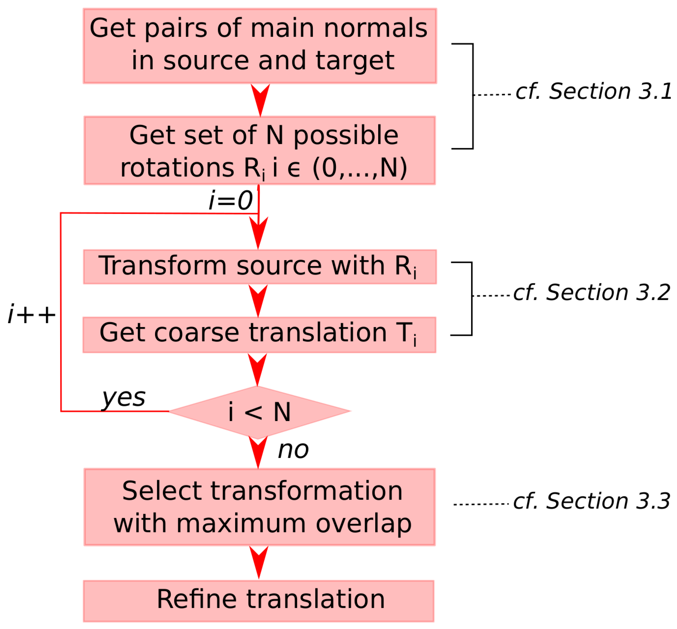
3. Structured Scene Feature-Based Registration

We have developed a method adapted to structured environments. The scene must contain planes, and the main walls of the target must have equivalences in the source. The algorithm associated with the method seeks to successively derive the rotation and the translation in two independent processes. The whole algorithm is presented in Algorithm 1. A simplified scheme of the pipeline is given in Figure 1.

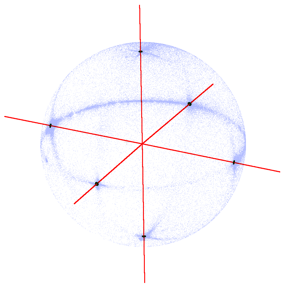
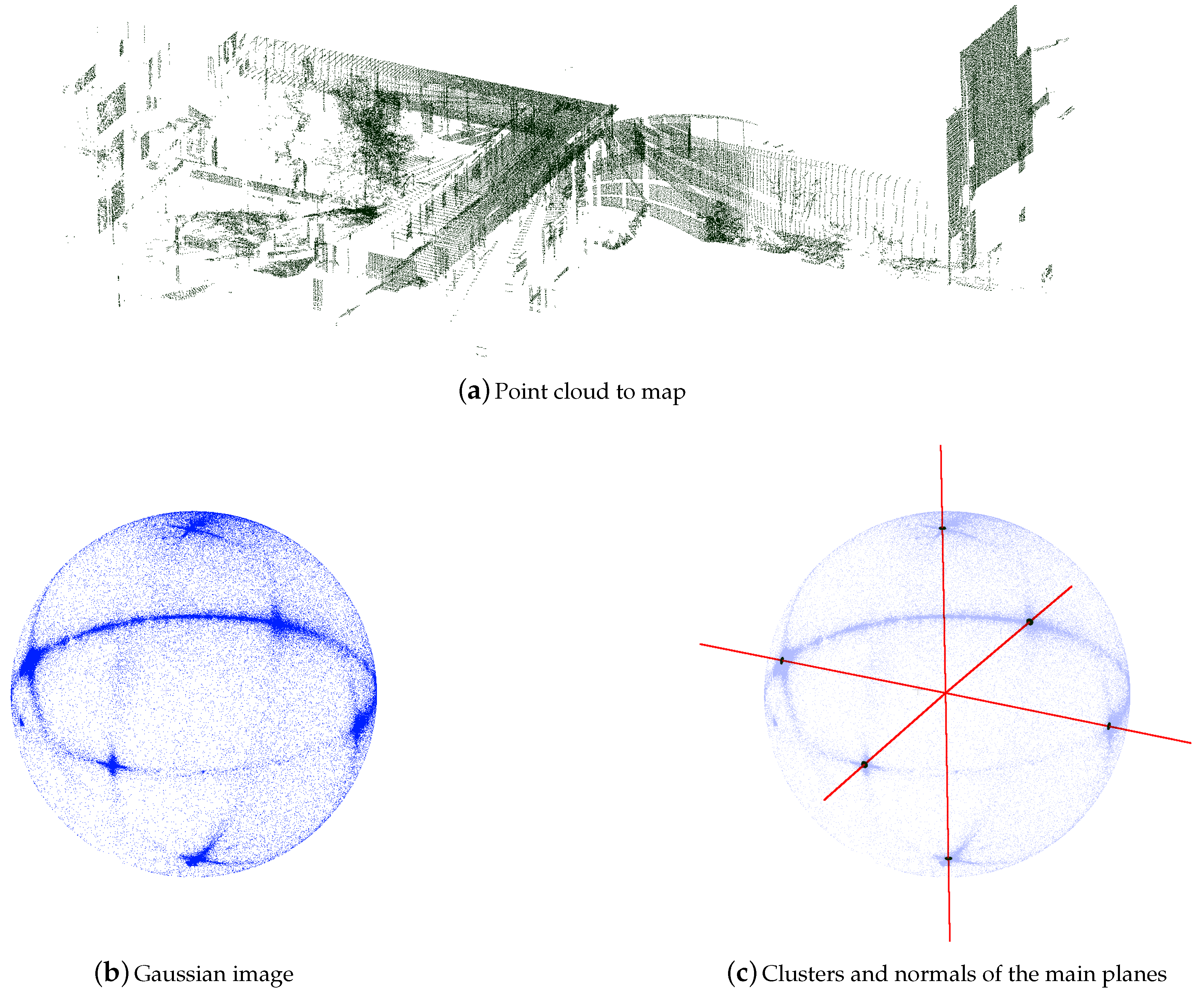
3.1. Rotation Search

The rotation search is summarized in Lines 1–10 of Algorithm 1.

3.1.1. Normal Computation

The first step consists of computing unit normals at each point for the source and for the target performing a principal component analysis in their neighborhoods. Then, the data are preprocessed with a uniform filter. A 3D grid is set on the point cloud, and one point per cell is kept.

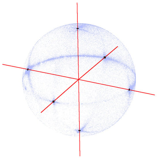
3.1.2. Gaussian Sphere Mapping

Then, both of the clouds are mapped onto the Gaussian sphere, i.e., the normals are represented as points on the unit sphere. One example of such a mapping is given in Figure 2. In this representation, the plane orientations are emphasized as the densest areas, but the distance information is lost. The main property of the Gaussian image is that the rotation impacts it in the same manner as the spatial representation [8]. The main idea of our method is based on the assumption that the environment is composed of a reasonable number of planes (walls, roof and ground) that we can detect in the Gaussian image and link between scans.

3.1.3. Density Filter

The next step consists of finding the main wall normals. The normals are first filtered to emphasize high density clusters on the Gaussian image as described below. The density is computed at each point as the number of neighbors in a defined radius $r_d$. Six areas of major density are selected successively as the six points with major density and their neighborhoods. We chose to limit the search to six main wall normals because this corresponds to the envelope of a basic room with four walls, the floor and the ceiling. These areas represent the clusters from which we want to extract the modes.

3.1.4. Mean Shift Process and Main Normals’ Selection

The modes representing the main walls’ normals are detected using a mean shift [35] algorithm with an Epanechnikov kernel [36]. The resulting modes are the main plane normals named $\overrightarrow{n_i}$ with $i=1,\dots ,N$, with N being the number of normals. An example of main normals’ selection is represented in Figure 2.

The detection quality depends on the radius $r_d$ of the density filter: a too small one can lead to misaligned clusters in the cases of large walls, while a too big one can make it impossible to detect clusters in the cases of small walls and makes the algorithm slower. It should be selected between 5 $\mathrm{m}\mathrm{m}$ and 10 $\mathrm{c}\mathrm{m}$ from the best normals’ quality to the worst.

The point clouds are filtered to keep all points on planes and reject all noisy points on non-significant objects. To perform this filtering, all points laying too far from the cluster modes on the Gaussian image are removed. A maximum angular error of ${10}^{\circ }$ is accepted.

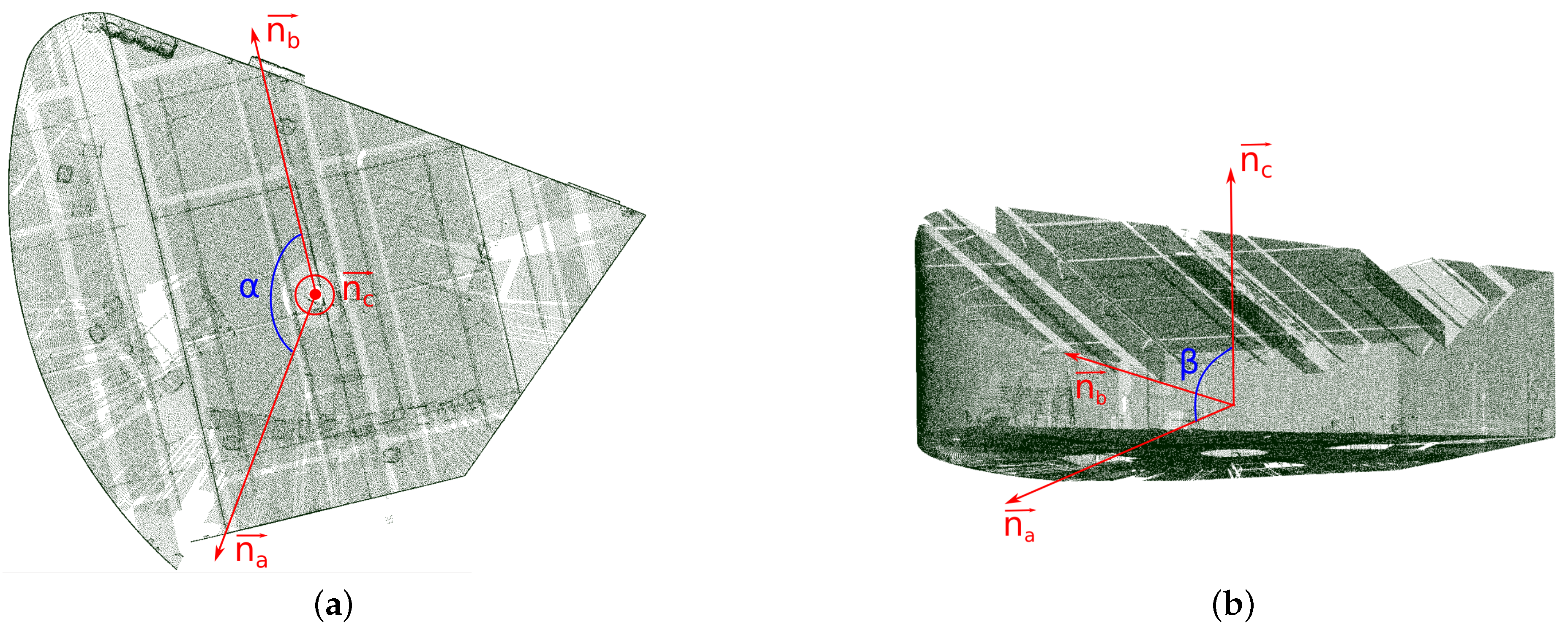
3.1.5. Creating Pairs of Normals and Matching

Once the two sets of main normals are obtained, all possible pairs of normals ${(\overrightarrow{n_i},\overrightarrow{n_j})}_T$, ${(\overrightarrow{n_k},\overrightarrow{n_l})}_S$ where $i,j=1,\dots ,N_T$ with $i\ne j$ and $k,l=1,\dots ,N_S$ with $k\ne l$ are formed with permutations respectively in the target (index T) and in the source (index S). The normals in a pair cannot be spatially opposed. The maximum number of pairs in one point cloud is $N_{pairs}=\frac{N!}{(N-2)!}$, with N the number of main normals encountered (up to six). The goal is then to link one pair of normals from the source with one pair of normals from the target. All possible correspondences between pairs are formed and then filtered, only keeping the pairs for which the angles $\widehat{{(\overrightarrow{n_i},\overrightarrow{n_j})}_T}$ and $\widehat{{(\overrightarrow{n_k},\overrightarrow{n_l})}_S}$ are similar, the error between both of the angles laying below a threshold. To find the best matching, all the remaining combinations are tested, and after the translation computation, the results of the whole registration are compared as explained in Section 3.3. The number of tests is lower than $M=\frac{N_S!}{(N_S-2)!}\times \frac{N_T!}{(N_T-2)!}$.

3.1.6. Rotation Computation

To compute the rotation in a closed form way between the matched pairs, the Singular Value Decomposition (SVD) is used [37] involving the two normal points on the unit sphere and the origin to remove translation movement.

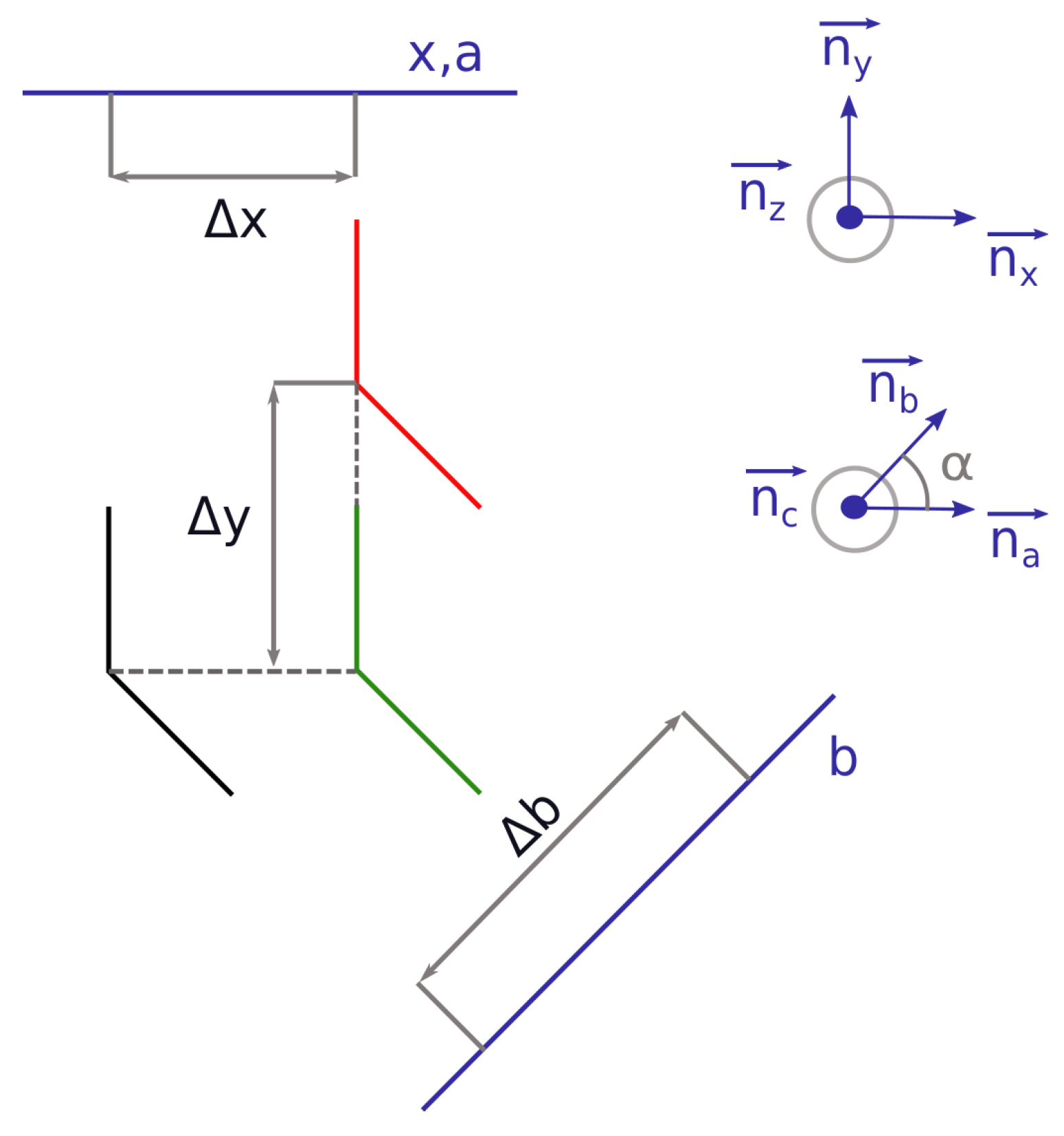
3.2. Translation Search

For each possible rotation, the computation of the translation is based on the building of histograms along the axis for both of the point clouds, as will be explained in this section.

3.2.1. Axes’ Selection

First, the translation axes are defined. This step corresponds to Line 11 of Algorithm 1. Three main normals, $\overrightarrow{n_a}$, $\overrightarrow{n_b}$, $\overrightarrow{n_c}$, are extracted from all modes computed for the target in the previous stage (described in Section 3.1). Two of them correspond to the normals used to perform the rotation in the previous step. The last one is derived after aligning the modes of the source and the target with the rotation. It corresponds to the mode of the target, outside the plane of the two previously selected ones, which is best aligned with one of the sources. These normals define the translation axes a, b, c. An example of axes’ selection is displayed in Figure 3.

3.2.2. Histograms’ Correlation

Secondly, the translation is derived through two steps involving one algorithm (summarized in Algorithm 2), which computes correlations of histograms from the source and histograms from the target. The point clouds are projected successively on each translation axis, and histograms are built from the projections. In the first step called step 1, the histograms are built with a large bin width to lead rapidly to a coarse translation alignment. This corresponds to Line 12 of Algorithm 1. In the second step, called step 2, the bin width is highly reduced, and the movement is limited inside the bin width of step 1 to lead to an accurate alignment. This corresponds to Line 20 of Algorithm 1. An explanation of this algorithm is detailed below.

Line 2: In both cases, the target and the rotated source are filtered and projected successively on the axes a, b, c. The filter allows, for each axis, to keep all points whose normal is parallel to the studied axis.

Line 3: A histogram is built on each axis for both point clouds.

Line 4: The histograms are filtered. The filter is different in step 1 and step 2. In step 1, the correlation is computed all along the translation axis. Therefore, the histograms must pass through a saturation stage to avoid having bins with a point number too large, which could corrupt the correlation step aligning the best observed wall respectively in the source context and in the target context at the expense of all walls pairs. In step 2, the bin width is small, and the walls are scattered throughout several bins. Then, a mean filter is applied to emphasize the walls in the histogram shape, revealing the densest regions.

Lines 5, 6 and 7: The maximum of the correlation between the histograms of a given axis corresponds to the convenient translation to apply to align the relative walls.

3.2.3. Translation Computation

Once the translations to perform on each axis are derived, the whole translation is computed. This step corresponds to Lines 9, 10 and 11 of Algorithm 2. Indeed, if the walls are perpendicular, and consequently a, b, c also are, the movements obtained can be directly applied on each axis. However, if the walls are not perpendicular, the movements are correlated one to the other. Then, a new orthogonal frame needs to be defined to lead to three independent translations. The axes of the new frame are named x, y, z and are represented by the vectors $\overrightarrow{n_x}$, $\overrightarrow{n_y}$, $\overrightarrow{n_z}$. They are defined as follows: $\overrightarrow{n_x}$ and $\overrightarrow{n_a}$ are superimposed; $\overrightarrow{n_z}$ is the cross product of $\overrightarrow{n_a}$ and $\overrightarrow{n_b}$; $\overrightarrow{n_y}$ is the cross product of $\overrightarrow{n_z}$ and $\overrightarrow{n_a}$. The movements on the axes a, b, c are called $\Delta a$, $\Delta b$ and $\Delta c$. The movements to compute on the x, y and z axes of the orthogonal local frame are called $\Delta x$, $\Delta y$ and $\Delta z$. A 2D representation of a two-wall configuration is displayed in Figure 4.

In this simplified figure, no movement is considered on the z axis. Equations (1) and (2) allow computing $\Delta x$ and $\Delta y$ with $\alpha$ the non-signed angle between the x and b axes. $\alpha$ belongs to the interval $[0,\pi ]$. The equivalence for the computation of the movement along the z axis is given by Equation (3) with $\beta$ the non-signed angle between the x and c axes and $\gamma$ the non-signed angle between the y and c axes. $\beta$ and $\gamma$ belong to the interval $[0,\pi ]$.

$$\Delta x=\Delta a$$

(1)

$$\Delta y=\frac{\Delta b-\Delta x\times cos\left(\alpha \right)}{sin\left(\alpha \right)}$$

(2)

$$\Delta z=\frac{\frac{\Delta c-\Delta x\times cos\left(\beta \right)}{sin\left(\beta \right)}-\Delta y\times cos\left(\gamma \right)}{sin\left(\gamma \right)}$$

(3)

3.3. Selection of Transformation

As described in Section 3.1, all rotations to align pairs of normals are tested. The corresponding coarse translations are computed, and the global transformations are compared to select the best one. To compare the results, the LCP (Largest Common Point-set) criterion [29] is used. It quantifies the overlap of the clouds. This value is the percentage of points of the source having at least one neighbor in the target, closer than a threshold radius. The threshold is defined as the point cloud resolution computed as the mean distance between each point and its closest neighbor. This step corresponds to Lines 14, 15 and 19 of Algorithm 1. After selection of the best transformation, the translation is refined using Algorithm 2 with a reduced bin width and computing the correlation in a limited interval. This process corresponds to Line 20 of Algorithm 1.

Algorithm 1: SSFR: Complete algorithm.

input target, source, r, rd, binWidth //r is the radius used to define the neighborhood to compute normals; $r_{\mathrm{d}}$ is the radius used to define the neighborhood to compute density

1: Compute normals with radius r and sample input clouds

2: Map $source$ and $target$ onto the Gaussian Sphere to get Gaussian images $G^{\mathrm{S}}$ and $G^{\mathrm{T}}$

3: Compute density at each point of $G^{\mathrm{S}}$ and $G^{\mathrm{T}}$ with radius $r_{\mathrm{d}}$

4: Extract the six densest regions from $G^{\mathrm{S}}$ and $G^{\mathrm{T}}$

5: Apply mean shift to find the modes $M_i^{\mathrm{S}}$ and $M_i^{\mathrm{T}}$ (with $i=1,\dots ,6$) from the densest regions

6: Make sets of pairs $P^{\mathrm{S}}$ and $P^{\mathrm{T}}$ with $M^{\mathrm{S}}$ and $M^{\mathrm{T}}$ elements // cf. Section 3.1

7: for all pair $P_j^{\mathrm{S}}\in P^{\mathrm{S}}$ do

8: for all pair $P_k^{\mathrm{T}}\in P^{\mathrm{T}}$ do

9:  if $P_j^{\mathrm{S}}.angle-P_k^{\mathrm{T}}.angle<ϵ$ then

10:    Get rotation $R_{jk}$ to align $P_j^{\mathrm{S}}$ on $P_k^{\mathrm{T}}$

11:    Select axes a, b, c from $M^{\mathrm{T}}$ // cf. Section 3.2

12:     Tjk ← GetTranslation(Rjk · source, target, a, b, c, binWidth) // cf. Algorithm 2

13:    Build global transformation matrix $A_{jk}\leftarrow T_{jk}·R_{jk}$

14:    Compute $LC{P}_{jk}$ between ($A_{jk}·source$) and $target$

15:    Append $LC{P}_{jk}$ to vector L and $A_{jk}$ to vector A

16:   end if

17:  end for

18: end for

19: $index\leftarrow argmax\left(L\right)$

20: Tjk ← GetTranslation(Aindex · source, target, a, b, c, binWidth/100) // cf. Algorithm 2

21: return Transformation matrix $M=T·A_{index}$

Algorithm 2: $GetTranslation$: Computation of the translation between the rotated source and the target.

input $rotatedSource$, $target$, a, b, c, $binWidth$ // a, b, c are the translation axes

1: for all $axis\in a,b,c$ do

2:  Filter $rotatedSource$ and $target$ and project points onto $axis$

3:  Compute histograms $his{t}_{axis}^{\mathrm{S}}$, $his{t}_{axis}^{\mathrm{T}}$

4:  Filter histograms

5:  Compute correlation $C_{axis}$

6:  $inde{x}_{axis}\leftarrow argmax\left(C_{axis}\right)$

7:  $\mathrm{\Delta }axis\leftarrow inde{x}_{axis}\times binWidth$

8: end for

9: $\mathrm{\Delta }x\leftarrow \mathrm{\Delta }a$

10: $\mathrm{\Delta }y\leftarrow \frac{\mathrm{\Delta }b-\mathrm{\Delta }x\times cos\left(\alpha \right)}{sin\left(\alpha \right)}$

11: $\mathrm{\Delta }z\leftarrow \frac{(\Delta c-\Delta x\times cos(\beta \left)\right)/sin\left(\beta \right)-\Delta y\times cos\left(\gamma \right)}{sin\left(\gamma \right)}$

12: return Translation matrix T with components $\mathrm{\Delta }x$, $\mathrm{\Delta }y$, $\mathrm{\Delta }z$

4. Materials and Methods

To evaluate our method, we used four datasets of LiDAR acquisitions corresponding to different scenes and application contexts. Some basic features of the four datasets are available in

Table 1. Datasets’ description: Dataset 1 ($DS1$-H)-Hokuyo, Dataset 2-Leica ($DS2$-L), Dataset 3-Velodyne ($DS2$-L), Dataset 4-Sick ($DS4$-S). Column “Points number” corresponds to the mean number of points per scan. Column “Max size” indicates the maximum distance between extreme points of the point clouds. Column “Resolution” corresponds to the mean resolution of the scans. Column “Motions” qualifies the movement between scans. The last column specifies if the ground truth transformations are available.

	Sensor	Scans Number	Points Number	Max size (m)	Resolution (cm)	Motions	Transformations
$DS1$-H	Hokuyo UTM-30LX	45	365,000	11	0.61	small	Yes
$DS2$-L	Leica P20	6	9 × 10−6	65	0.35	large	Yes
$DS3$-V	Velodyne HDL-32E	41	56,000	120	7.70	small	No
$DS4$-S	SICK LMS-200	63	81,600	25	8.20	small	No

.

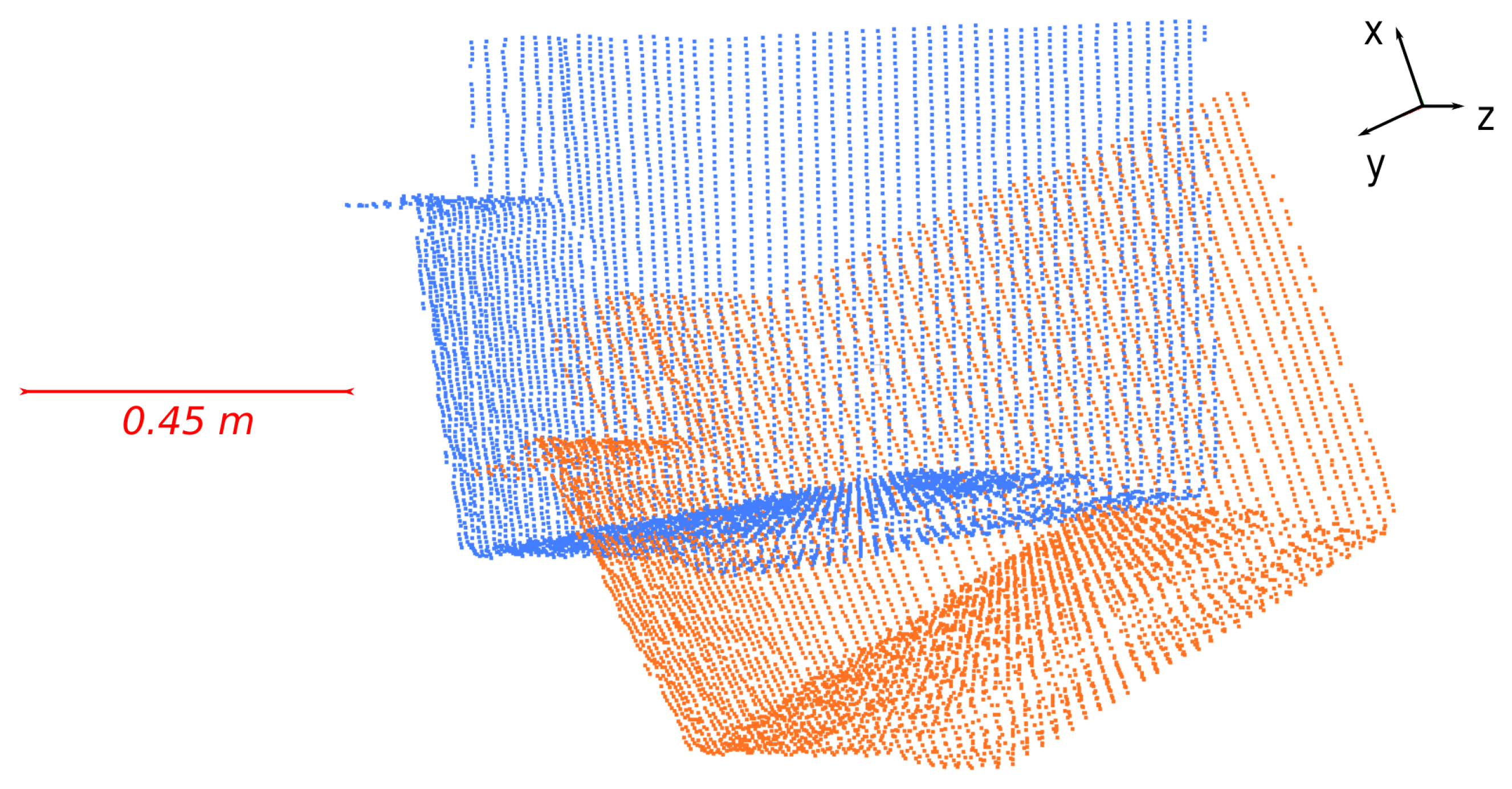
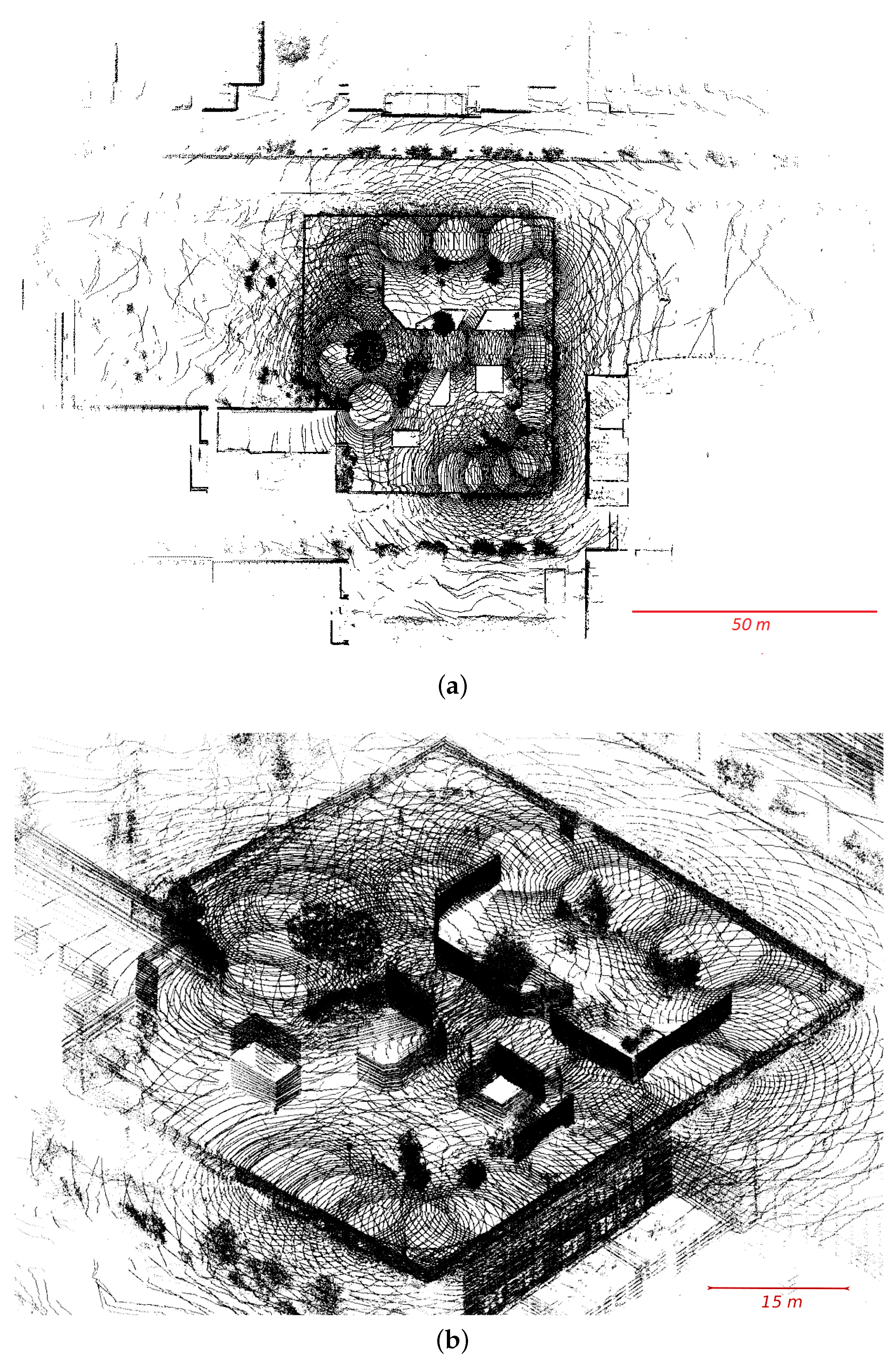
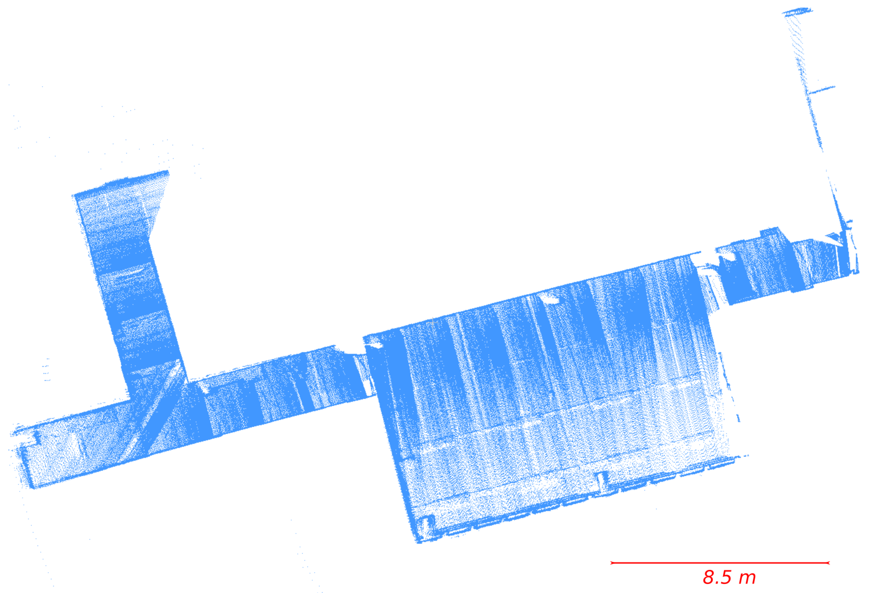
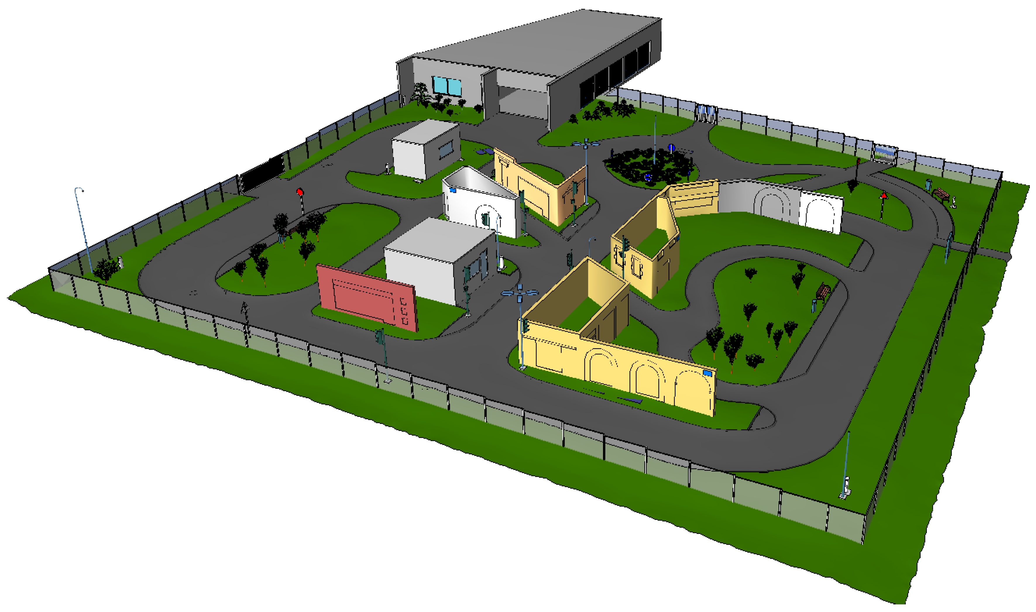
4.1. Dataset 1: Hokuyo

The first dataset is named “apartment” and is available online on the ASL (Autonomous System Lab) website [38]. It has been acquired by the Swiss Federal Institute of Technology in Zürich to test the robustness of algorithms when exploring a dynamic environment. Indeed, some objects are moved between scan acquisitions. The Hokuyo sensor used for this dataset acquisition provides a good accuracy (±3 $\mathrm{c}\mathrm{m}$), and a precise map of the scene could be reconstructed from the data. Its detection range reaches 30 $\mathrm{m}$. It rotates around a vertical axis to get an aperture angle of ${270}^{\circ }$. For more details, see the constructor website [39]. It was mounted on a tilted device with a controlled motor to get 3D scans, and a theodolite was used to estimate the ground truth poses. This dataset is referenced as $DS1$-H (Dataset 1-Hokuyo) in this work.

4.2. Dataset 2: Leica

We acquired the second dataset at the Institut Pascal of Clermont-Ferrand to exploit data of an indoor environment with more complexity and to be able to compare to a ground truth. It is referenced as $DS2$-L (Dataset 2-Leica) in this study. It was acquired with a Leica scanner, which allows obtaining very good accuracy and information up to 120 meters away from the sensor with measurements in interval angles of ${360}^{\circ }$ horizontally and ${270}^{\circ }$ vertically. This scanner is recommended to perform a good scene reconstruction with an accuracy of ±3 $\mathrm{m}\mathrm{m}$ 50 $\mathrm{m}$ away and leads to a detailed representation. For further information about the sensor, see the constructor website [40]. This dataset contains six scans, numbered from 0–5, of a two-floor building with many windows. It can be qualified as a complex environment as it contains complex structures such as an outdoor view of trees, curved walls and stairs. Moreover, its size can reach 65 $\mathrm{m}$ from one extremity to the other. The ground truth poses were acquired using physical targets.

4.3. Dataset 3: Velodyne

The third dataset was also captured at the Institut Pascal from a Velodyne HDL-32E LiDAR sensor, which provides distance measurements in interval angles of ${360}^{\circ }$ horizontally and ${40}^{\circ }$ vertically (using 32 lasers rotating around a vertical axis). Such a Velodyne sensor is largely used for robotic applications including autonomous vehicle control and mobile terrestrial mapping. It provides 3D point cloud data at a high refresh rate (10 $\mathrm{Hz}$) and a long range (100 m). Its typical accuracy is ±2 $\mathrm{c}\mathrm{m}$. For more details, see the constructor website [41]. The outdoor scene is a structured circuit: the PAVIN site (Plateforme d’Auvergne pour Véhicules Intelligents). A scheme of this scene is given in Figure 5. The sensor was mounted on a mobile vehicle to obtain 3D measurements. We chose to acquire these data to evaluate the robustness of our algorithm in the context of navigation. Forty scans were extracted from the complete dataset (1 scan over 100). This dataset is referenced as $DS3$-V (Dataset 3-Velodyne) in this study.

4.4. Dataset 4: Sick

This last dataset, referenced as $DS4$-S (Dataset 4-Sick), was acquired at the University of Osnabrück [42] on the website [43]. It was acquired with a SICK LMS-200 laser sensor mounted on a robot to acquire 3D measurements with a movement of ${180}^{\circ }$ horizontally and ${100}^{\circ }$ vertically and a typical accuracy of ±1.5 $\mathrm{c}\mathrm{m}$. For more details, see the constructor website [44]. This dataset is particularly challenging due to the noise introduced by the movement of the robot and the small angular aperture of the scanner.

4.5. Evaluation Tools

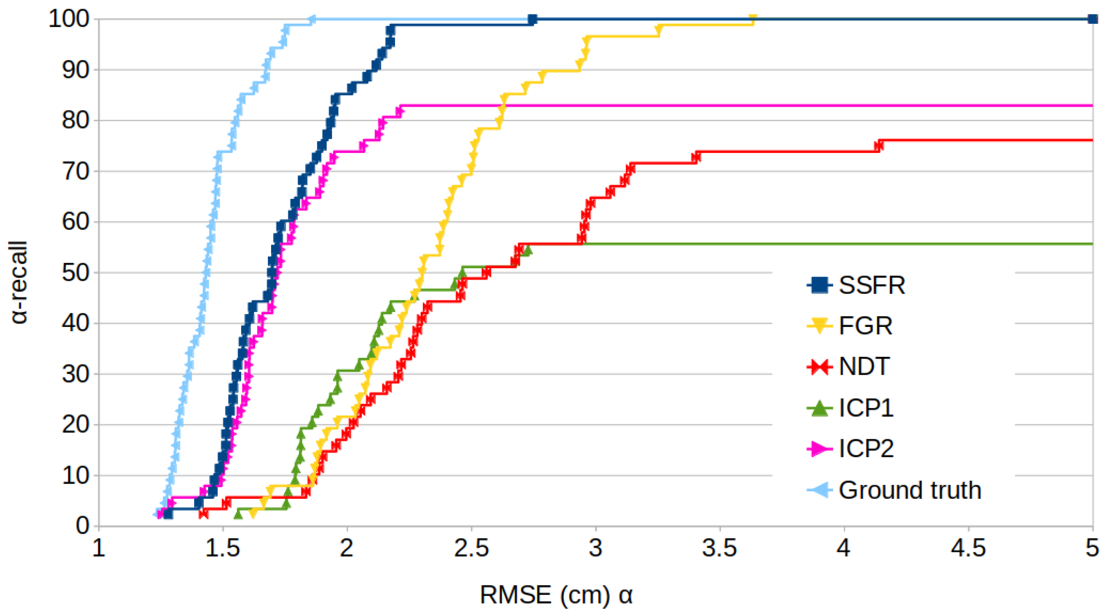
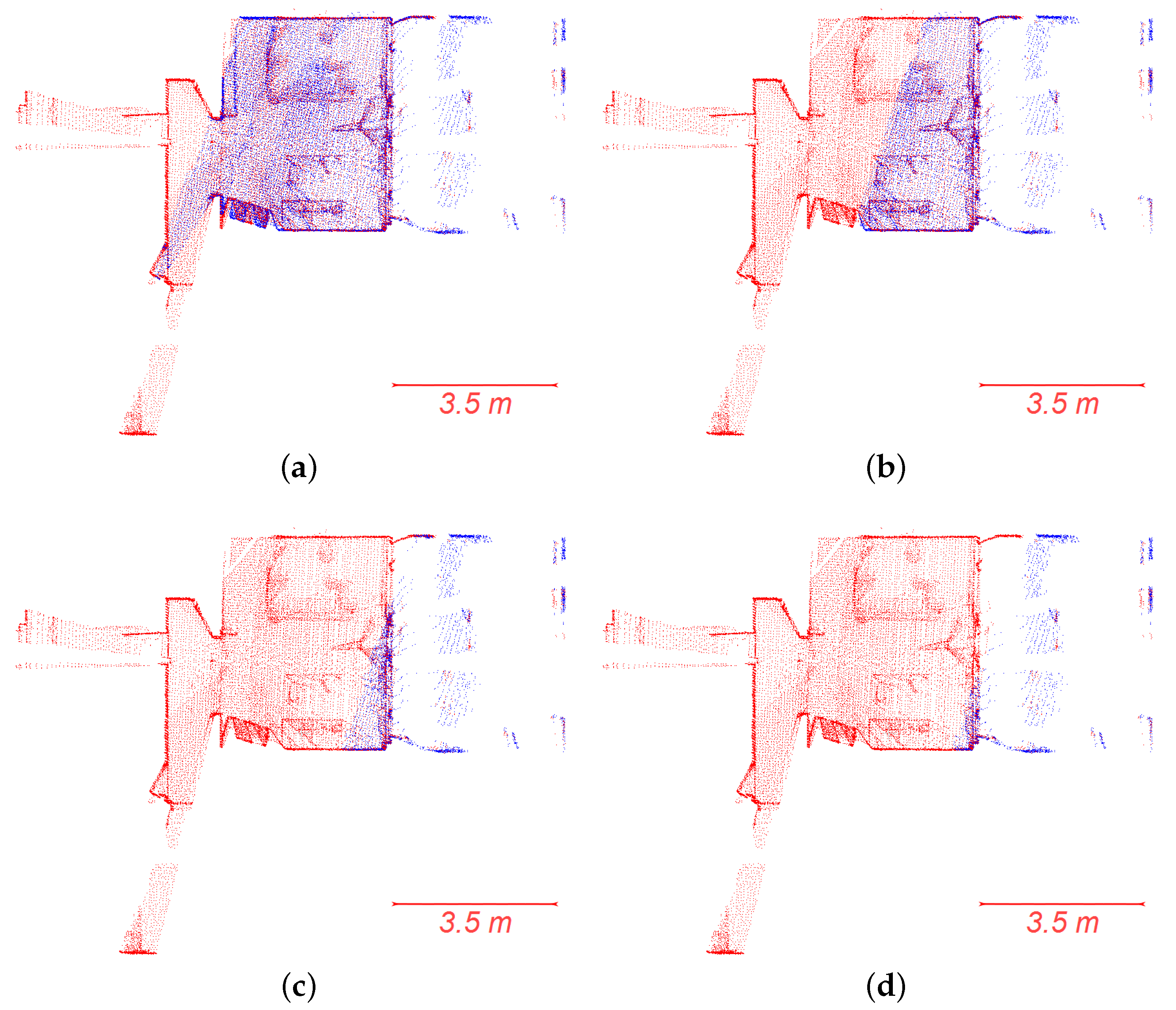
To validate the results of the registration, we used several criteria. First, we evaluated the Root Mean Square Error (RMSE) between source and target. The correspondences between points were established searching for the nearest neighbor of each target point in the source after transformation. To deal with the overlap issue in this association, a threshold was chosen to reject outliers in the matching pairs as suggested by Lehtola et al. in their study about the evaluation of point clouds’ reconstruction [45]. However, in our case, this threshold is set as the resolution of the point cloud. The RMSE value depends on the resolution of the clouds and needs to be compared to the reference RMSE computed with the ground truth transformation.

Secondly, the translation error and the rotation error are examined. The rotation error is represented as the combination of three rotation angles around the axes of the global frame. The success rate is also studied and is defined as the percentage of registrations that have an RMSE lower than 10 $\mathrm{c}\mathrm{m}$. Besides, we studied the computation time of our algorithm (processor: 8 cores Intel Xeon-E5620, 2.4 $\mathrm{G}\mathrm{Hz}$). We chose to compare our method with six well-known algorithms: ICP point-to-point, ICP point-to-plane, NDT, FGR, Super4PCS and Go-ICP. The ICP and NDT algorithms were implemented using Point Cloud Library (PCL); FGR, Go-ICP and Super4PCS were tested using the code supplied by the authors. Before entering each algorithm, the point clouds are uniformly sampled, the normals are calculated with the same radius parameter and aberrant points are removed. The running times only include the registration process.

5. Results

5.1. Basic Model

First, a subset of real data from $DS1$-H was used. This extract was sampled uniformly to contain 7000 points and moved with a defined transformation T to obtain a second point cloud. The result of this process is shown in Figure 6. The two point clouds hence overlap completely. The RMSE and the computation time were studied for all methods listed above and reported in

Table 2. Comparison of the methods on a part of real data representing a corner of a room and containing 7000 points. ICP1: ICP point-to-point; ICP2: ICP point-to-plane; NDT: Normal Distribution Transform; FGR: Fast Global Registration. $T_1$, $T_2$ and $T_3$ are rotations over the z axis with respectively ${20}^{\circ }$, ${45}^{\circ }$, ${90}^{\circ }$. x represents the situation in which the algorithm did not converge.

		${\mathit{T}}_1$		${\mathit{T}}_2$		${\mathit{T}}_3$
	Parameters Number	RMSE (cm)	T (s)	RMSE (cm)	T (s)	RMSE (cm)	T (s)
ICP1	1	4.23 × 10−4	0.2	x	x	x	x
ICP2	2	3.77 × 10${}^{-\mathbf{5}}$	0.2	3.70 × 10${}^{-\mathbf{5}}$	0.2	x	x
NDT	1	1.29 × 10−1	2.2	x	x	x	x
FGR	3	1.54 × 10−3	0.5	1.74 × 10−3	0.6	2.78 × 10−5	0.6
Super4PCS	2	5.83	1.7	9.65	11.1	3.30	3.1
Go-ICP	4	5.77 × 10−4	41.5	3.31 × 10−4	42.0	1.83 × 10${}^{-\mathbf{5}}$	82.4
SSFR	3	2.70 × 10−3	0.3	3.98 × 10−3	0.3	3.36 × 10−4	0.3

. The transformations, called $T_1$, $T_2$ and $T_3$, are rotations over the z axis. The first one corresponds to a rotation of ${20}^{\circ }$; the second one corresponds to a rotation of ${45}^{\circ }$; and the last one to a rotation of ${90}^{\circ }$. The normals are computed with a radius of neighborhood of 10 $\mathrm{c}\mathrm{m}$ for each point. No sampling is performed. For the SSFR method, we used a density radius of 5 $\mathrm{m}\mathrm{m}$.

In this case, we can notice that our algorithm cannot find the exact transformation compared to ICP methods. However, it gets a reliable RMSE and is one of the fastest. It is to be noted that the result of our algorithm and its computation time do not depend on the initial movement between the point clouds, and we still get reliable results when ICP or NDT methods do not converge. Super4PCS does not obtain an accurate result because it needs an ICP refinement, and its computation time is not constant due to its random process. Go-ICP obtains the best results regardless of the rotation applied on the input. However, its long computation time for 7000 points allows one to think that it cannot be used for large data such as indoor environment scans.

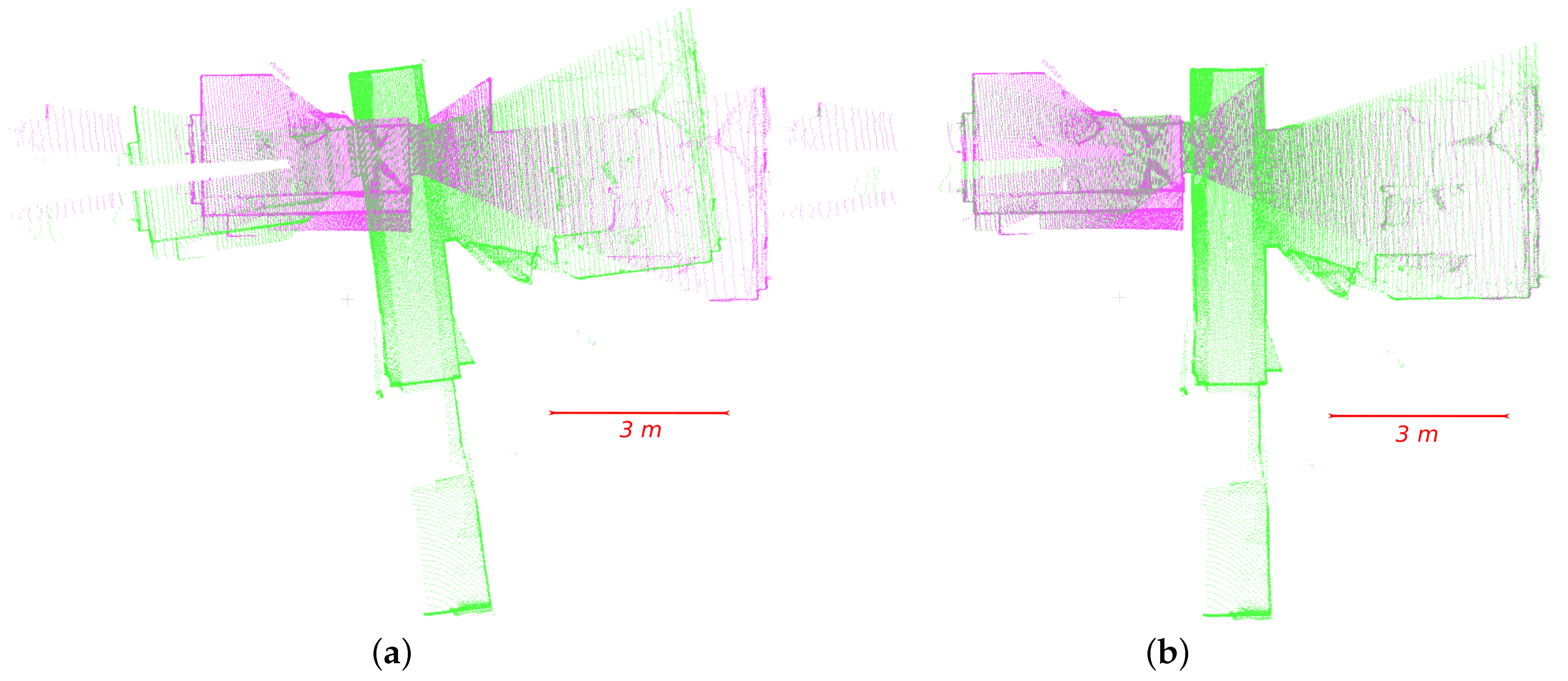
5.2. Indoor Environment

Then, we evaluated our algorithm on $DS1$-H (cf. Section 4.1), acquired with a Hokuyo sensor, to test its robustness in the context of scene reconstruction in an indoor environment. For all methods, the radius of the neighborhood for the calculation of normals was set to 10 $\mathrm{c}\mathrm{m}$. Then, the point clouds were uniformly sampled using a grid to obtain a mean resolution of 3.6 $\mathrm{c}\mathrm{m}$, which corresponds to an average of 23,000 points per scan. An example of the registration process with our algorithm is represented in Figure 7.

The RMSE results of our algorithm SSFR are reported in Figure 8 through an $\alpha$-recall graph and in

Table 3. Evaluation of the SSFR method on $DS1$-H. Comparison with methods ICP1, ICP2, NDT, FGR. nd: no data.

	RMSE (cm)	Success Rate (%)	Time (s)
ICP1	2.0	54	7.4
ICP2	1.7	82	3.2
NDT	2.4	61	5.2
FGR	2.3	100	3.9
SSFR	1.8	100	2.4
GT	1.4	100	nd

. For this experiment, the radius of the neighborhood to compute density in our method is set to 1 $\mathrm{c}\mathrm{m}$. SSFR is compared to the ICP point-to-plane, FGR and NDT methods. ICP point-to-point and ICP point-to-plane are performed with a filter for correspondences based on distance. They are applied first with a rejecting distance of 30 $\mathrm{c}\mathrm{m}$ and secondly with a rejecting distance of 15 $\mathrm{c}\mathrm{m}$. The grid length for the NDT method was set to 40 $\mathrm{c}\mathrm{m}$. For NDT, ICP point-to-point and ICP point-to-plane, iterations are stopped when the variation of the transformation matrix elements is under a threshold of 1 × 10⁻⁶. FGR is performed with a division factor of $1.1$, the tuple scale is set to $0.95$, and the number of correspondences used is set to 10,000. The FPFH features are computed with a radius of 40 $\mathrm{c}\mathrm{m}$.

We notice that the SSFR algorithm reaches the accuracy of ICP point-to-plane on this dataset. Moreover, the ICP point-to-plane algorithm fails in $15\%$ of the cases due to a large motion between the scans. The NDT and ICP point-to-point methods have low performances on this dataset. The FGR algorithm appears to be less accurate than the SSFR method, but has a success rate of 100%. Super4PCS’s results are not displayed here because the performances were low without a refinement stage. Moreover, the Super4PCS and Go-ICP algorithms are too long to be applied in the context of this environment with more than 10,000 points. They were stopped after 10 min of running.

We aimed to evaluate the robustness of our algorithm against a decrease of the point clouds’ sampling. Therefore, we sampled the input clouds with a uniform filter and evaluated the RMSE of the ICP point-to-plane, FGR and SSFR algorithms. For this experiment, the radius of the neighborhood to compute density is set to 2 $\mathrm{c}\mathrm{m}$ to emphasize the effect of the points’ number on the density filter. The results are presented in

Table 4. Evaluation of the robustness of the studied algorithms against the sampling rate of the point clouds in $DS1$-H. Points are sampled with a uniform filter. SR: Success Rate.

	ICP Point-to-Plane			FGR			SSFR
Resolution (cm)	SR (%)	RMSE B	Time (s)	SR (%)	RMSE (cm)	Time (s)	SR (%)	RMSE (cm)	Time (s)
2.6	81.8	1.7	8.7	100	2.2	9.7	100	1.8	25.7
3.6	81.8	1.7	3.1	100	2.3	4.2	100	1.8	13.1
4.6	84.1	1.7	1.5	100	2.6	3.2	100	1.9	7.2
5.9	79.5	1.8	0.9	100	3.0	1.8	100	1.9	4.4
10.6	75.0	1.8	0.2	93.2	5.1	1.2	100	2.1	0.6
16.0	59.0	1.9	0.06	65.9	6.2	2.0	100	2.5	0.3

. The FPFH features are computed with a radius of 60 $\mathrm{c}\mathrm{m}$ for the two cases with the biggest sampling rates in order to get the best results.

We notice that the SSFR algorithm is robust against weak resolutions of the input data with a success rate of 100% regardless of the resolution and an RMSE comparable to the ICP method until a resolution of 5.9 $\mathrm{c}\mathrm{m}$. Table 4 also shows that the running time of our algorithm increases rapidly with the number of points; cf. the discussion in Section 6. We also aimed to evaluate the density radius parameter impact on the results. Then, we evaluated the RMSE for different radius values. The results are available in

Table 5. Evaluation of the SSFR algorithm, on $DS1$-H, varying the radius for density computation.

Radius (cm)	RMSE (cm)	Time (s)
0.1	2.1	0.7
0.5	1.8	1.0
1	1.8	2.4
2	1.8	6.5
3	1.8	6.1
4	1.8	11.0
6	1.8	15.3
10	1.8	24.2

. It shows that the radius has a weak impact on the RMSE in $DS1$-H, but it has a significant impact on the run time, increasing it 30-times.

In order to evaluate the robustness of our algorithm against the weak overlap, SSFR algorithm was tested on scans from $DS1$-H, trimming one of the scans to reduce the overlap. The overlap is evaluated using an LCP value with a threshold of 10 $\mathrm{c}\mathrm{m}$ as defined in Section 3.3. A representation of four different configurations is given in Figure 9.

Our algorithm solves the registration until LCP = 6% (cf. Figure 10). For LCP = 5% (cf. Figure 9d), SSFR gives the wrong alignment. This is due to the disappearance of one wall, which makes the translation search fail. The ICP algorithm solves the registration problem until a minimum overlap of 12% (cf. Figure 9c). The FGR algorithm gets to the same result as SSFR in this experiment.

5.3. Complex Indoor Environment

We aimed to evaluate our SSFR method on a more complex environment. Therefore, a complete study of all the criteria defined in the introduction of Section 4 was done on $DS2$-L acquired with a Leica LiDAR scanner (cf. Section 4.2). The point clouds were first sampled uniformly to get an average of 41,000 points per scan. At the end, they have a resolution between 5 $\mathrm{c}\mathrm{m}$ and 7 $\mathrm{c}\mathrm{m}$. The radius of the neighborhood for normals’ computation is set to 10 $\mathrm{c}\mathrm{m}$. Then, the radius relative to density computation $r_d$ was set to 8 $\mathrm{m}\mathrm{m}$ based on the good accuracy of normals and the large number of points. An example of the result of our algorithm is displayed in Figure 11. We evaluated the resulting transformations on the initial clouds sampled to get a resolution between 2.7 $\mathrm{c}\mathrm{m}$ and 3.1 $\mathrm{c}\mathrm{m}$. The results are presented in

Table 6. Evaluation of results on $DS2$-L. RMSE GT: RMSE computed after Ground Truth transformation. RMSE: RMSE after the resulting transformation. Registrations on the left are denoted as A_B, where A is the reference number of the source and B the reference number of the target.

	RMSE GT (cm)	RMSE (cm)	Translation Error (cm)	Rotation Errors (${}^{\circ }$)	Time (s)
1_0	2.66	2.73	0.006	0.023, 0.025, 0.024	15.8
2_1	2.68	2.99	1.0	0.035, 0.045, 0.021	23.5
3_2	2.83	3.37	1.7	0.065, 0.008, 0.037	27.1
4_3	2.58	2.59	0.001	0.0006, 0.04, 0.006	19.8
5_4	2.55	2.61	0.0007	0.008, 0.015, 0.039	33.9
Average	2.66	2.91	0.54	0.026, 0.027, 0.025	24.0

.

The accuracy is reliable, although a weak rotation error of some hundredths of degree can introduce an RMSE of various millimeters. The rotation error comes from the normal calculation, the precision of the parallelism of walls in the real scene and the mean shift process accuracy. All other methods previously mentioned in Section 4 were tested on this dataset, but none of them get to a close result of registration.

We can obtain a result with a weak loss of accuracy and a significant gain of time by sampling uniformly the input to a coarser resolution. For example, with a mean resolution of 11.7 $\mathrm{c}\mathrm{m}$, we obtained a mean RMSE of 3.0 $\mathrm{c}\mathrm{m}$ with a mean duration of 6.8 $\mathrm{s}$ per registration.

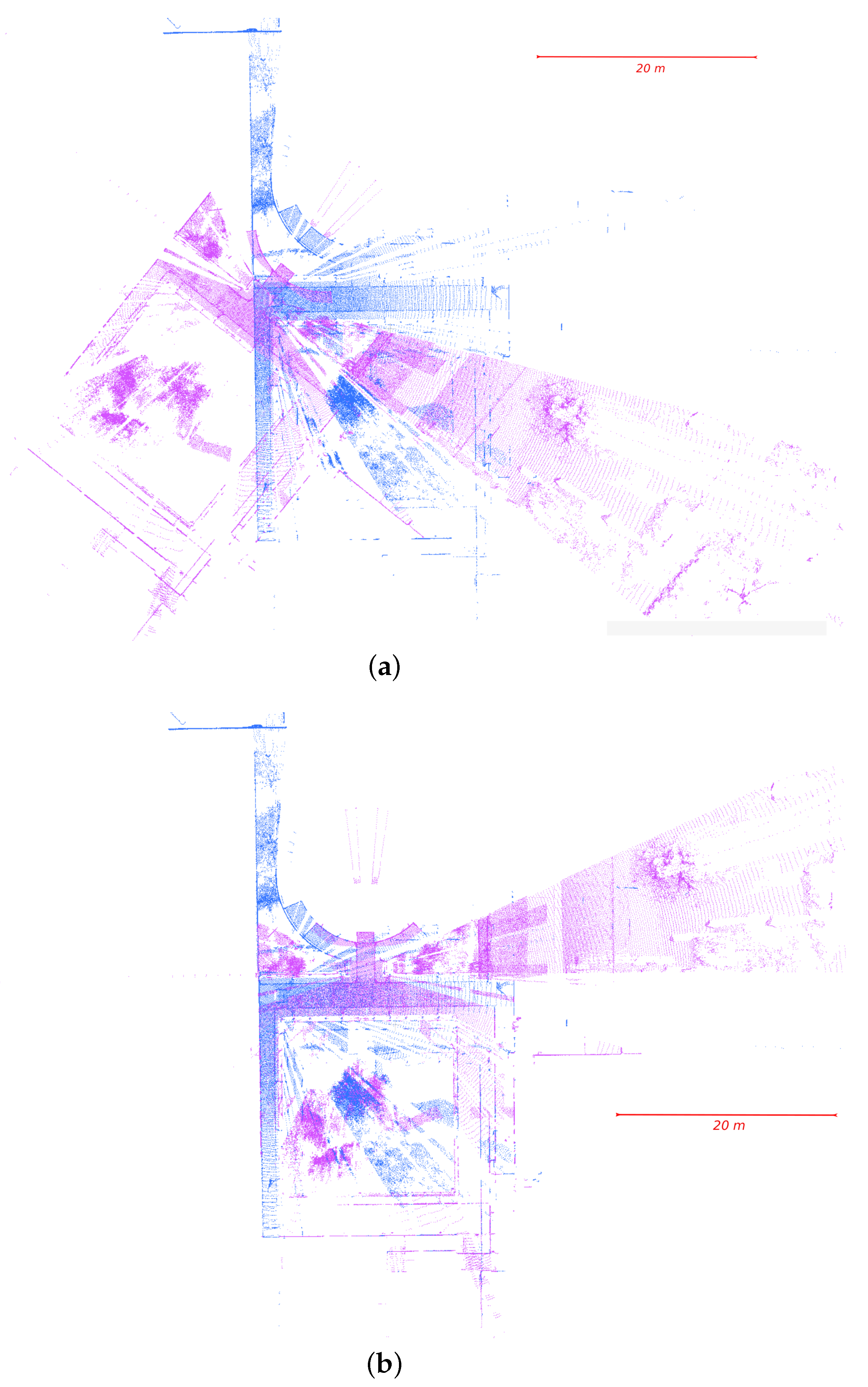
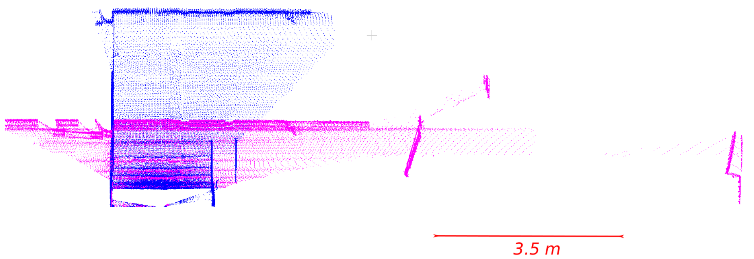
5.4. Navigation Context

We also wanted to evaluate our SSFR method on a less detailed environment for an application in the navigation process. Therefore, we tested on $DS3$-V, (cf. Section 4.3). It contains 4100 scans acquired at a frequency of 10 $\mathrm{Hz}$. We used one scan over 100 and obtained 40 registrations. This dataset is composed of scans acquired in motion, which adds a difficulty to the registration because the origin moves during one scan acquisition. Methods may be applied to correct the scans before registration [46], but in this example, we did not use any correction. The whole result is displayed in Figure 12. To evaluate the results, we used the closed loop. Indeed, we selected two scans, one at the beginning of the loop and one at the end of the loop. Then, we compared the direct registration between the two scans with the serial registration using the intermediate scans. The first registration is complemented with an ICP step to get an accurate reference. The normal radius r was set to 80 $\mathrm{c}\mathrm{m}$ due to the weak resolution of the farthest planes. The density radius $r_d$ was set to 6 $\mathrm{c}\mathrm{m}$ because of the poor quality of normals. We obtained an RMSE between source and target correspondent points of 27.4 $\mathrm{c}\mathrm{m}$ after the serial registrations, whereas the direct registration has an RMSE of 3.2 $\mathrm{c}\mathrm{m}$. We can conclude that the actual average error is 1.2 $\mathrm{c}\mathrm{m}$ per registration. The average time for a registration is 16 $\mathrm{s}$. We compared the ICP and FGR methods to ours on this dataset and evaluated the success rate of the registrations. The results are available in

Table 7. Evaluation of the SSFR method on $DS3$-V. Comparison with methods ICP1, ICP2 and FGR.

	Success Rate (%)
ICP1	12
ICP2	20
FGR	85
SSFR	100

. ICP was applied first with a rejecting distance of 5 $\mathrm{m}$ and then with a rejecting distance of 50 $\mathrm{c}\mathrm{m}$. FGR was used with a division factor of $1.1$, a tuple scale of $0.95$ and a maximum number of correspondences of 10,000, and the radius for FPFH computation was set to 1 $\mathrm{m}$.

5.5. Failure Cases

To show the limitations of our algorithm, we tested it on another challenging dataset $DS4$-S provided by the University of Osnabrück. In Figure 13, a part of the dataset has been registered with the SSFR algorithm. Eighty-eight percent of the scans can be successfully registered by our algorithm. Some failure cases appear. An example of failure is given in Figure 14, where two scans were not well aligned due to their poor overlap and because they do not include enough points on correspondent walls.

6. Discussion

The results obtained in Section 5 show that our algorithm is robust in various acquisitions contexts. In this section, we emphasize the advantages and limitations of our method.

In Table 3, we notice that our algorithm is the most accurate (RMSE of 1.8 $\mathrm{c}\mathrm{m}$ for a ground truth RMSE of 1.4 $\mathrm{c}\mathrm{m}$) when evaluated on all registration cases. It is also the fastest with a mean running time of 2.4 $\mathrm{s}$ per registration. Table 5 reports the effect of varying $r_d$ on the resulting RMSE. This experiment shows that this radius has a weak impact on the RMSE when passing a threshold linked to the accuracy of normals. In this experiment, this threshold is around 1 $\mathrm{m}\mathrm{m}$. However, it has a significant impact on the computation time increasing it 10-times. If the quality of the normals is weak, a compromise must be found by the user to set this parameter in order to get a minimum running time remaining away from the threshold. Moreover, Table 4 shows that our method is robust when varying the resolution of the point clouds from 2.6 $\mathrm{c}\mathrm{m}$–16.0 $\mathrm{c}\mathrm{m}$. The computation time is significantly reduced (25.7 $\mathrm{s}$–0.3 $\mathrm{s}$), and the RMSE remains below 2.5 $\mathrm{c}\mathrm{m}$. However, this experiment also shows that the running time of our algorithm increases rapidly with the number of points. This is due to the density filter and the mean shift algorithm used in the rotation search (cf. Section 3.1), which have a complexity of $\mathcal{O}\left(n^2\right)$. Therefore, this method could be used if a coarse alignment is expected in a limited time or if an accurate alignment is expected in a greater time. For comparison, FGR cannot solve all the registrations of $DS1$-H with a resolution greater than 10 $\mathrm{c}\mathrm{m}$ (93%) and has a bad success rate (66%) for a resolution of 16 $\mathrm{c}\mathrm{m}$. The overlap experiment proves that our algorithm is robust when decreasing the overlap between the source and the target. For the example given in Figure 9, we noticed that SSFR can solve the registration until the overlap gets to 5%.

The experiment on $DS2$-L proves that our algorithm is more robust than existing ones on complex indoor environments provided by laser scanners as Leica. The running times found in Table 6 would enable a real-time implementation.

With the evaluation on $DS3$-V, we show that the SSFR algorithm can solve the registration with noisy data without further preprocesses than a uniform filter. The noise comes from the Velodyne sensor, which has an accuracy of ±2 $\mathrm{c}\mathrm{m}$, and from points 100 $\mathrm{m}$ away from the sensor, which make the normals’ computation more difficult due to their poor resolution. It also comes from the movement of the vehicle during sensor acquisitions.

Nevertheless, our algorithm cannot solve the registration problem when it cannot identify three walls with different orientations in a point cloud. This is the case for long corridors where only two main directions can be extracted (walls and floor/ceiling). Another problem can appear when the three main walls of the scene are not shared between the two scans. An example is given in Figure 14, where two scans were not well aligned due to their poor overlap and because they do not include points on common walls in three directions. These limits lead to some failure cases of registration in $DS4$-S (seven cases). It is to be noted that, in this challenging dataset, the points are particularly noisy because of the poor accuracy of the sensor, and noise is added by the movement of the scanner during acquisition, making the computation of normals more complicated without preprocessing. The horizontal aperture angle is smaller (${180}^{\circ }$) than in other datasets (${360}^{\circ }$), making the overlap between scans weaker.

Our method is the only one working on all the presented datasets. It reaches a reliable accuracy on simply-structured indoor environments, but it also solves registration problems on complex indoor environments and on outdoor structured environments with motion and fewer details. The runtime depends on the sampling of the points, but also on the quality of normals. It remains fast enough to perform a real-time registration in the context of building reconstruction, and as it is robust to subsampling, it can be combined with an ICP refinement to be faster and more accurate, entering with greater resolutions.

7. Conclusions

In this study, we presented a new algorithm for the global registration of structured scenes with partial overlap without the use of odometric data or physical targets. It is based on geometric features of indoor scenes, and it leads to a reliable accuracy for complex environments. Its speed allows one to consider a real-time implementation in the context of building reconstruction. This algorithm works without initial alignment and can be used on scenes with fewer details because it does not use local descriptors. Its non-iterative process leads to reliable results within a limited time. It constitutes a good compromise between computation time and accuracy, ensuring a result close to reality regardless of the input data sampling. It was evaluated on four datasets that have been acquired with different LiDAR sensors. Two of them were acquired for the purpose of this study at the Institut Pascal. Our method appears to be robust against noisy acquisitions since it can solve the registration problem with uniformly-filtered data without any further preprocess. An evaluation of the robustness against a weak overlap shows that our algorithm reaches the performance of the newest methods. In future work, we plan to expand the database created at the moment to process more challenging indoor configurations. Moreover, a work on scene modeling after registration will be conducted using the extraction of planes proposed in this method, in order to enhance high level primitives.

References

1. Ochman, S.; Vock, R.; Wessel, R.; Klein, R. Automatic reconstruction of parametric building models from indoor point clouds. Comput. Graph. (Pergamon) 2016, 54, 94–103. [Google Scholar] [CrossRef]
2. Reu, J.; De Smedt, P.; De Herremans, D.; Van Meirvenne, M.; Laloo, P.; De Clercq, W. On introducing an image-based 3D reconstruction method in archaeological excavation practice. J. Archaeol. Sci. 2014, 41, 251–262. [Google Scholar] [CrossRef]
3. Cadena, C.; Carlone, L.; Carrillo, H.; Latif, Y.; Scaramuzza, D.; Neira, J.; Reid, I.; Leonard, J.J. Past, Present, and Future of Simultaneous Localization and Mapping: Toward the Robust-Perception Age. IEEE Trans. Robot. 2016, 32, 1309–1332. [Google Scholar] [CrossRef]
4. Han, J.Y. A non-iterative approach for the quick alignment of multistation unregistered LiDAR point clouds. IEEE Geosci. Remote Sens. Lett. 2010, 7, 727–730. [Google Scholar] [CrossRef]
5. Besl, P.; McKay, N. A Method for Registration of 3-D Shapes. IEEE Trans. Pattern Anal. Mach. Intell. 1992, 14, 239–256. [Google Scholar] [CrossRef]
6. Brou, P. Using the Gaussian Image to Find the Orientation of Objects. Int. J. Robot. Res. 1984, 3, 89–125. [Google Scholar] [CrossRef]
7. Horn, B.K.P. Extended Gaussian images. Proc. IEEE 1984, 72, 1671–1686. [Google Scholar] [CrossRef]
8. Kang, S.B.; Ikeuchi, K. Determining 3-D object pose using the complex extended Gaussian image. In Proceedings of the IEEE Computer Society Conference on Computer Vision and Pattern Recognition (CVPR), Maui, HI, USA, 3–6 June 1991; pp. 580–585. [Google Scholar]
9. Makadia, A.; Patterson, A.I.; Daniilidis, K. Fully automatic registration of 3D point clouds. In Proceedings of the 2006 IEEE Computer Society Conference on Computer Vision and Pattern Recognition CVPR, New York, NY, USA, 17–22 June 2006; Volume 1, pp. 1297–1304. [Google Scholar]
10. Pomerleau, F.; Colas, F.; Siegwart, R.; Magnenat, S. Comparing ICP Variants on Real-World Data Sets. Auton. Robots 2013, 34, 133–148. [Google Scholar] [CrossRef]
11. Pomerleau, F.; Colas, F.; Siegwart, R. A Review of Point Cloud Registration Algorithms for Mobile Robotics. Found. Trends Robot. 2015, 4, 1–104. [Google Scholar] [CrossRef]
12. Zhang, Z. Iterative point matching for registration of free-form curves and surfaces. Int. J. Comput. Vis. 1994, 13, 119–152. [Google Scholar] [CrossRef]
13. Segal, A.; Haehnel, D.; Thrun, S. Generalized-ICP. Robot. Sci. Syst. 2009, 5, 168–176. [Google Scholar]
14. Fitzgibbon, A.W. Robust Registration of 2D and 3D Point Sets. Image Vis. Comput. 2002, 21, 1145–1153. [Google Scholar] [CrossRef]
15. Gruen, A.; Akca, D. Least squares 3D surface and curve matching. ISPRS J. Photogramm. Remote Sens. 2005, 59, 151–174. [Google Scholar] [CrossRef]
16. Yang, J.; Li, H.; Jia, Y. Go-ICP: Solving 3D registration efficiently and globally optimally. In Proceedings of the 2013 IEEE International Conference on Computer Vision (ICCV), Sydney, Australia, 1–8 December 2013; pp. 1457–1464. [Google Scholar]
17. Gelfand, N.; Ikemoto, L.; Rusinkiewicz, S.; Levoy, M. Geometrically stable sampling for the ICP algorithm. In Proceedings of the 4th International Conference on 3-D Digital Imaging and Modeling, Banff, Alberta, AB, Canada, 6–10 October 2003; pp. 260–267. [Google Scholar]
18. Borrmann, D.; Elseberg, J.; Lingemann, K.; Nüchter, A.; Hertzberg, J. Globally consistent 3D mapping with scan matching. Robot. Auton. Syst. 2008, 56, 130–142. [Google Scholar] [CrossRef]
19. Holz, D.; Ichim, A.E.; Tombari, F.; Rusu, R.B.; Behnke, S. Registration with the Point Cloud Library: A Modular Framework for Aligning in 3-D. IEEE Robot. Autom. Mag. 2015, 22, 110–124. [Google Scholar] [CrossRef]
20. Filipe, S.; Alexandre, L.A. A comparative evaluation of 3D keypoint detectors in a RGB-D Object Dataset. In Proceedings of the 2014 International Conference on Computer Vision Theory and Applications (VISAPP), Lisbon, Portugal, 5–8 January 2014; Volume 1, pp. 476–483. [Google Scholar]
21. Rusu, R.B.; Blodow, N.; Beetz, M. Fast Point Feature Histograms (FPFH) for 3D registration. In Proceedings of the IEEE International Conference on Robotics and Automation, Kobe, Japan, 12–17 May 2009; pp. 3212–3217. [Google Scholar]
22. Johnson, A.E.; Hebert, M. Using spin images for efficient object recognition in cluttered 3D scenes. IEEE Trans. Pattern Anal. Mach. Intell. 1999, 21, 433–449. [Google Scholar] [CrossRef]
23. Tombari, F.; Salti, S.; Di Stefano, L. Unique Signatures of Histograms for Local Surface Description. In Proceedings of the European Conference on Computer Vision (ECCV), Heraklion, Greece, 5–11 September 2010; pp. 356–369. [Google Scholar]
24. Han, J.; Perng, N.; Lin, Y. Feature Conjugation for Intensity Coded LiDAR Point Clouds. IEEE Geosci. Remote Sens. Lett. 2013, 139, 135–142. [Google Scholar] [CrossRef]
25. Wang, F.; Ye, Y.; Hu, X.; Shan, J. Point cloud registration by combining shape and intensity contexts. In Proceedings of the 9th IAPR Workshop on Pattern Recognition in Remote Sensing (PRRS), Cancun, Mexico, 4 December 2016; Volume 139, pp. 1–6. [Google Scholar]
26. Zhou, Q.-Y.; Park, J.; Koltun, V. Fast Global Registration. In Proceedings of the Computer Vision—ECCV 2016: 14th European Conference, Amsterdam, The Netherlands, 11–14 October 2016; Volume 2, pp. 766–782. [Google Scholar]
27. Fischler, M.A.; Bolles, R.C. Paradigm for Model. Commun. ACM 1981, 24, 381–395. [Google Scholar] [CrossRef]
28. Aiger, D.; Mitra, N.J.; Cohen-or, D. 4-Points Congruent Sets for Robust Pairwise Surface Registration. ACM Trans. Graph. (SIG-GRAPH) 2008, 27, 10. [Google Scholar]
29. Mellado, N.; Aiger, D.; Mitra, N.J. Super 4PCS fast global pointcloud registration via smart indexing. Comput. Graph. Forum 2014, 33, 205–215. [Google Scholar] [CrossRef]
30. Magnusson, M.; Lilienthal, A.; Duckett, T. Scan registration for autonomous mining vehicles using 3D-NDT. J. Field Robot. 2007, 24, 803–827. [Google Scholar] [CrossRef] [Green Version]
31. Magnusson, M. The Three-Dimensional Normal-Distributions Transform—An Efficient Representation for Registration, Surface Analysis, and Loop Detection. Ph.D. Thesis, Orebro University, Örebro, Sweden, 2009. [Google Scholar]
32. Breitenreicher, D.; Schnörr, C. Model-based multiple rigid object detection and registration in unstructured range data. Int. J. Comput. Vis. 2011, 92, 32–52. [Google Scholar] [CrossRef]
33. Pathak, K.; Vaskevicius, N.; Birk, A. Uncertainty analysis for optimum plane extraction from noisy 3D range-sensor point-clouds. Intell. Serv. Robot. 2009, 3, 37–48. [Google Scholar] [CrossRef]
34. Pathak, K.; Birk, A. Fast Registration Based on Noisy Planes with Unknown Correspondences for 3D Mapping. IEEE Trans. Robot. 2010, 26, 424–441. [Google Scholar] [CrossRef]
35. Cheng, Y. Mean shift, mode seeking, and clustering. IEEE Trans. Pattern Anal. Mach. Intell. 1995, 17, 790–799. [Google Scholar] [CrossRef]
36. Epanechnikov, V. Nonparametric estimation of a multidimensional probability density. Theory Probab. Appl. 1969, 14, 153–158. [Google Scholar] [CrossRef]
37. Sorkine-Hornung, O.; Rabinovich, M. Least-Squares Rigid Motion Using SVD; Technical Report; ETH Department of Computer Science: Zürich, Switzerland, 2017. [Google Scholar]
38. Pomerleau, F.; Liu, M.; Colas, F.; Siegwart, R. Challenging data sets for point cloud registration algorithms. Int. J. Robot. Res. 2012, 31, 1705–1711. [Google Scholar] [CrossRef]
39. Hokuyo Website. Available online: www.hokuyo-aut.jp (accessed on 27 September 2017).
40. Leica Website. Available online: w3.leica-geosystems.com (accessed on 27 September 2017).
41. Velodyne Website. Available online: www.velodynelidar.com (accessed on 27 September 2017).
42. Elseberg, J.; Borrmann, D.; Lingemann, K.; Nüchter, A. Non-Rigid Registration and Rectification of 3D Laser Scans. In Proceedings of the 2010 IEEE/RSJ International Conference on Intelligent Robots and Systems, Taipei, Taiwan, 18–22 October 2010; pp. 1546–1552. [Google Scholar]
43. Nüchter, A.; Lingemann, K. Robotic 3D Scan Repository. Available online: kos.informatik.uos.de/3Dscans/ (accessed on 27 September 2017).
44. SICK Website. Available online: www.sick.com (accessed on 27 September 2017).
45. Lehtola, V.V.; Kaartinen, H.; Nüchter, A.; Kaijaluoto, R.; Kukko, A.; Litkey, P.; Honkavaara, E.; Rosnell, T.; Vaaja, M.T.; Virtanen, J.P.; et al. Comparison of the Selected State-Of-The-Art 3D Indoor Scanning and Point Cloud Generation Methods. Remote Sens. 2017, 9, 796. [Google Scholar] [CrossRef]
46. Vivet, D.; Checchin, P.; Chapuis, R. Localization and Mapping Using Only a Rotating FMCW Radar Sensor. Sensors 2013, 13, 4527–4552. [Google Scholar] [CrossRef] [PubMed]
Figure 1. Schematic pipeline of the whole SSFR algorithm.
Remotesensing 09 01014 g001
Figure 2. Main wall normals’ detection: (a) point cloud to map; (b) mapping of normals onto the Gaussian sphere; (c) the remaining clusters after the density filter appear in black, and the main plane normals are depicted in red. The normals are selected through a mean shift process to find clusters of points and their modes.
Remotesensing 09 01014 g002
Figure 3. Selection of translation axes in the scan of a room. The scan was acquired with a Leica LiDAR scanner at Institut Pascal Clermont-Ferrand (France). The axes come from an analysis of the scene normals. (a) Seen from above; (b) seen from one side.
Remotesensing 09 01014 g003
Figure 4. Schematic scene seen from above, of a two-wall translation from an initial position (black) to a final position (red). In green, the walls are represented after their translation along the x axis.
Remotesensing 09 01014 g004
Figure 5. PAVIN site (Plateforme d’Auvergne pour Véhicules Intelligents) scheme. A Velodyne sensor, mounted on top of a vehicle, is moved along the road and acquires scans with a frequency of 10 Hz .
Remotesensing 09 01014 g005
Figure 6. Basic model to register. Subset of points from Scan 2 of D S 1 -H. The initial point cloud is represented in orange, and the result of its rotation of 20 around the z axis is represented in blue.
Remotesensing 09 01014 g006
Figure 7. Example of registration with the SSFR algorithm on D S 1 -H. Scan 4 (green) is aligned on Scan 3 (magenta). (a) Before registration; (b) after registration.
Remotesensing 09 01014 g007
Figure 8. Experiments on D S 1 -H. α -recall is the percentage of tests for which a given method achieves an RMSE < α . Higher is better. Comparison with algorithms: ICP1, ICP2, FGR and NDT.
Remotesensing 09 01014 g008
Figure 9. Scans 6 and 7 from D S 1 -H used to test the robustness of algorithms against weak overlap. Scan 7 is trimmed to reduce the overlap. For good visibility, the scans are aligned with the ground truth transformation. The overlap is expressed with the Largest Common Point-set (LCP) value (cf. Section 3.3). (a) LCP = 68%; (b) LCP = 34%; (c) LCP = 12%; (d) LCP = 5%.
Remotesensing 09 01014 g009
Figure 10. Successful registration with the SSFR algorithm of Scan 7 (trimmed) on Scan 6 from D S 1 -H for a current LCP of 6%.
Remotesensing 09 01014 g010
Figure 11. Example of registration with the SSFR algorithm on D S 2 -L. Scan 1 (magenta) aligned on Scan 0 (blue). (a) Before registration; (b) after registration.
Remotesensing 09 01014 g011
Figure 12. PAVIN site after reconstruction using D S 3 -V. The algorithm works only from the sequence of scans without the use of any proprioceptive sensor. Only 18 over the 40 scans are represented for a good visibility of the scene. (a) Seen from above; (b) seen from one side.
Remotesensing 09 01014 g012
Figure 13. Part of reconstruction of a building located in the Osnabrück University using our method on 19 scans from D S 4 -S.
Remotesensing 09 01014 g013
Figure 14. Failed registration with our algorithm SSFR on scans from D S 4 -S. There are not enough points on walls shared between scans to make the algorithm work.
Remotesensing 09 01014 g014