Article

UAS-SfM for Coastal Research: Geomorphic Feature Extraction and Land Cover Classification from High-Resolution Elevation and Optical Imagery

1
U.S. Geological Survey, Woods Hole, MA 02543, USA
2
Marine Biological Laboratory, Woods Hole, MA 02543, USA
3
Woods Hole Analytics, Woods Hole, MA 02543, USA
4
U.S. Geological Survey, St. Petersburg, FL 33701, USA
*
Author to whom correspondence should be addressed.
Remote Sens. 2017, 9(10), 1020; https://doi.org/10.3390/rs9101020
Submission received: 25 July 2017 / Revised: 16 September 2017 / Accepted: 26 September 2017 / Published: 3 October 2017
(This article belongs to the Section Remote Sensing in Geology, Geomorphology and Hydrology)

Abstract

:
The vulnerability of coastal systems to hazards such as storms and sea-level rise is typically characterized using a combination of ground and manned airborne systems that have limited spatial or temporal scales. Structure-from-motion (SfM) photogrammetry applied to imagery acquired by unmanned aerial systems (UAS) offers a rapid and inexpensive means to produce high-resolution topographic and visual reflectance datasets that rival existing lidar and imagery standards. Here, we use SfM to produce an elevation point cloud, an orthomosaic, and a digital elevation model (DEM) from data collected by UAS at a beach and wetland site in Massachusetts, USA. We apply existing methods to (a) determine the position of shorelines and foredunes using a feature extraction routine developed for lidar point clouds and (b) map land cover from the rasterized surfaces using a supervised classification routine. In both analyses, we experimentally vary the input datasets to understand the benefits and limitations of UAS-SfM for coastal vulnerability assessment. We find that (a) geomorphic features are extracted from the SfM point cloud with near-continuous coverage and sub-meter precision, better than was possible from a recent lidar dataset covering the same area; and (b) land cover classification is greatly improved by including topographic data with visual reflectance, but changes to resolution (when <50 cm) have little influence on the classification accuracy.

Graphical Abstract

1. Introduction

Coastal environments are highly dynamic systems that change in response to wind, waves, tides, storms, and long-term sea-level. Short-term and long-term changes important to understanding the processes and timescales driving the evolution of the coast are measured through ongoing monitoring and observations, provided largely by remotely sensed imagery and elevation data. Positional changes in alongshore features such as the shoreline and foredunes [1,2] can be used to quantify rates of change and to assess the spatial variability of these features [3]. Rates of change can be related to other factors such as the geologic framework [4,5,6], sediment supply [7], and human modifications [8,9]. Land cover change analysis allows us to map the evolution of the landscape such as development, expansion, and translation of marsh extent [10], as well as identifying habitat changes that affect beach-dependent species, such as the federally-listed piping plover (Charadrius melodus) [11]. Updating these metrics before and immediately after storms, and over time (weeks, seasons, years) provides critical information to better understand storm impacts [12], preferential site characteristics, interannual cycles [13], and the overall morphologic and ecologic resilience of these dynamic environments to longer-term drivers such as sea-level change [14].
Frequent data collection is needed to measure and monitor ongoing coastal change and evaluate habitat use in these systems, but repeat surveys can be costly, time-consuming, and involve working in sensitive or restricted environments [15]. Vantage points, coverage, and access can be limited in ground-based surveys due to variable terrain, vegetation, and habitat sensitivity, and storm impacts can compound access issues through erosion, overwash, or breaching, making direct measurements difficult. Although there are remote sensing techniques that can alleviate many of the ground-based limitations (e.g., airborne lidar and satellite imagery) [16], the platforms and data are expensive or provide coverage at an unsuitable temporal or spatial resolution for small-scale site-specific observation [17]. As a result, areas of interest are often surveyed using multiple techniques to assess change over a range of timescales [18].
Unmanned Aerial Systems (UAS; sometimes referred to as drones) coupled with Structure-from-Motion (SfM) photogrammetry offer a rapidly mobilized, and underutilized coastal surveying alternative that can provide high-resolution aerial coverage to quickly assess storm impacts and monitor recovery [17,19]. In this study, we evaluate the ability of these systems to map and measure coastal features in areas with sandy shores and semi-vegetated dunes. We first use SfM to generate a three-dimensional point cloud, a gridded digital elevation model (DEM), and a georeferenced orthomosaic image for a representative coastal site. We then determine the applicability of these products for use in coastal research by calculating the horizontal and vertical accuracy of elevations. We derive shoreline and foredune positions from the point cloud, and classify land cover using the orthomosaic and DEM. Finally, we evaluate the influence of data density and processing resolution on the extraction of beach geomorphic features using established methods, as well as the influence of resolution and use of topographic data on classification accuracy.

2. Materials and Methods
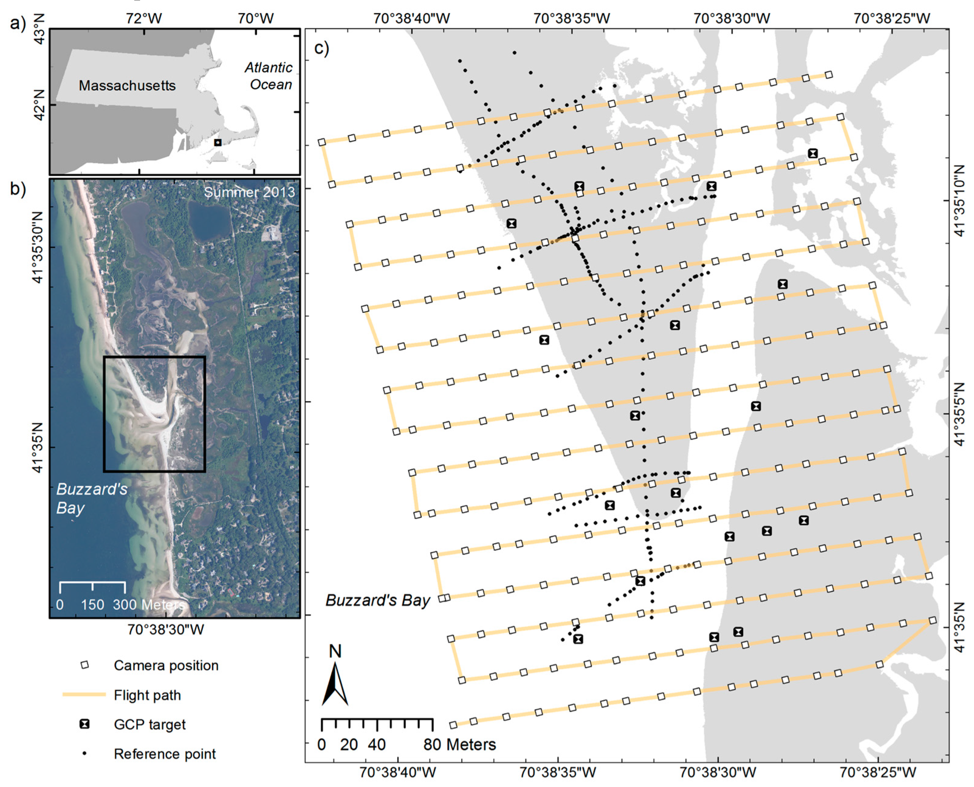
The field data and first-level products are distributed with detailed processing steps in the published data [20]. Figure 1 shows the general workflow undertaken in this project.

2.1. Study Area

Black Beach is a west-facing coastal beach that rises to semi-vegetated dunes and shelters a salt marsh from the waters of Buzzards Bay, Massachusetts, USA (Figure 2). The general components of the Black Beach system, including a dynamic shoreline, foredunes, and a range of vegetation, are typical of coastal systems globally and make it a suitable test site for generating the two coastal analysis products emphasized in this study. The positions of geomorphic features, such as those present at Black Beach (i.e., shoreline, dune toe, and dune crest), are fundamental measures used globally for coastal vulnerability assessment [21,22]. In addition, the array of land cover at this site is characteristic of beaches on the U.S. mid- to south-Atlantic coast, and constitutes critical habitat for conservation.
A small tidal inlet to Great Sippewissett Marsh bisects the study area. Tides are semidiurnal with a range of about 1.3 m; the mean high water (MHW) elevation is 0.66 m and the local mean sea level (MSL) is 0.13 m (all elevations in this study are referenced to North American Vertical Datum of 1988 (NAVD88)) [23]. Waves generally approach from southwest during summer, and west to northwest during the winter. The beach is characterized by medium- to coarse-grained sand, with ephemeral lags of glacial cobbles exposed on the foreshore and lower intertidal zone. The frontal dune is generally continuous and up to 3.5 m, and is covered with Ammophila breviligulata grass of varying density. Secondary and tertiary dunes exhibit elevations up to 3.7 m, are less continuous, and include a variety of vegetation including both dune grasses and woody vegetation. The adjacent salt marsh vegetation is dominated by Spartina alterniflora in the low marsh (0.25 m–0.5 m), by S. alterniflora mixed with S. patens around MHW, and by S. patens and Distichlis spicata in the high marsh [24,25].
On average, this portion of the Buzzards Bay shoreline is undergoing a long-term retreat of about 0.15 ± 0.03 m/yr [26,27] and Black Beach and Great Sippewissett Inlet display decadal-scale fluctuations in position and morphology around this long-term trend. In the last 35 to 55 years, the shoreline has retreated about 30 m with accompanying dune retreat [28]. These geomorphological changes have consequences for habitat. Black Beach and the adjacent Great Sippewissett Marsh are designated as Priority Habitat of Rare Species by the Massachusetts Natural Heritage and Endangered Species Program (NHESP) in part because the beach is used by beach-nesting shorebirds including the least tern (Sternula antillarum) and the piping plover (Charadrius melodus), a federally-listed threatened species [29].

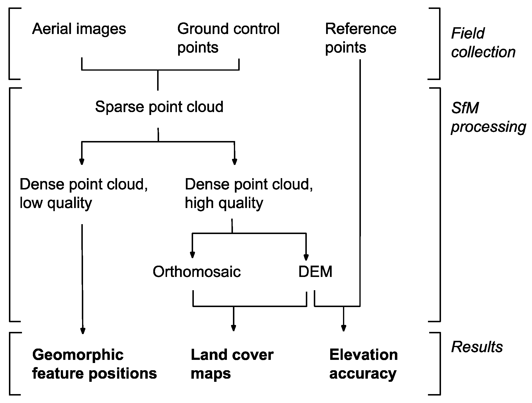
2.2. UAS-SfM Processing

2.2.1. Field Data Collection

A DJI Phantom 3 Professional (Dà Jiāng Innovations Science and Technology Co., Ltd., Shenzhen, China) quadcopter collected 250 images (12 megapixel JPEG files) with a near-nadir look angle during two flights at approximately 35 m altitude on 18 March 2016 between approximately 1100 and 1130 EDT. Skies were cloud-free and wind speeds were about 10 m/s. The built-in camera sensor captured an image approximately every 20 m in 15 east–west transects spaced 30 m apart (Figure 2). Image footprints have 80% overlap with 2.5 cm pixel resolution and cover an area of approximately 300 m × 500 m. The approximate camera position at the time of each photograph was measured by a global navigation satellite system (GNSS) receiver on-board the quadcopter and recorded in the header of the image file [20].
Immediately prior to the aerial survey, we placed 18 black and white 1-m2 targets and surveyed the positions of their center points for use as ground control points (GCPs). Coincident with the quadcopter flights, we surveyed 254 reference points at roughly 5-m intervals along two north–south transects and six east–west transects over the principal terrestrial area. Surveying was performed with three Spectra Precision SP80 GNSS receivers (Trimble Inc., Sunnyvale, CA, USA) connected to the Massachusetts Continuously Operating Reference Station (MaCORS) real-time kinematic (RTK) GNSS network. Horizontal positions were referenced to World Geodetic Datum of 1984 (WGS84)/Universal Transverse Mercator (UTM) Zone 19N and vertical positions were referenced to NAVD88, Geoid 12A. The GCPs had an average horizontal error of 1.1 cm and vertical error of 1.4 cm and the entire set of surveyed points had an average horizontal error of 0.9 cm and vertical error of 1.3 cm [20].

2.2.2. Structure-from-Motion

Georeferenced visual-topographic point clouds, a DEM, and an orthomosaic were produced using SfM algorithms in Agisoft PhotoScan Professional (v1.2.6, Agisoft LLC, St. Petersburg, Russia). SfM workflows are well-established [19,30,31] and are minimally elaborated here. Detailed processing steps, including optimization parameters, are presented in Table A1 and distributed in the published data [20].
The SfM workflow to generate a point cloud includes photo alignment and tie point generation, camera optimization, geo-registration to GCPs and finally dense point cloud construction (Table A1). The software first corrects image distortion and then uses a multi-view stereo reconstruction procedure to place each pixel in XYZ space. This results in elevation point clouds that are 3-dimensional positions with associated color information (red-green-blue (RGB) values). PhotoScan allows the user to customize in the Build Dense Cloud tool whether and by how much to downscale the images during processing.
We created both a high- and low-density point cloud to address processing limitations. The high-density point cloud was created after downscaling the input images to 50% (high quality setting in PhotoScan) and the low-density cloud was created after downscaling the images to 12.5% (low quality setting) [32]. The low-density version was created for use in geomorphic feature extraction because existing software routines created for lidar point clouds could not tolerate the large file size and extremely high data density of the high-density cloud.
The high-density point cloud was used to create the orthomosaic and DEM (Figure 3) in PhotoScan. We first eliminated points that were clearly isolated from the landscape surface by viewing the point cloud from different angles. Most of these points were associated with areas of water and were caused by glint or other photographic artifacts. The updated point cloud was converted to a DEM with a resolution of 5 cm × 5 cm using an Inverse Distance Weighted algorithm for interpolation. The orthomosaic image was created by projecting the orthorectified photos, at their original resolution, over the DEM using PhotoScan’s mosaic blending mode [33].

2.3. Derived Products

The SfM products were evaluated for topographic error and were used to derive two second-level datasets: beach geomorphic feature positions and a classified land cover surface. We resampled the SfM products to a variety of resolutions and ran the processes with each of the resampled datasets. We then compared the differences in accuracy that resulted from changes to the input parameters.

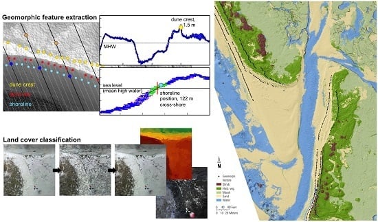
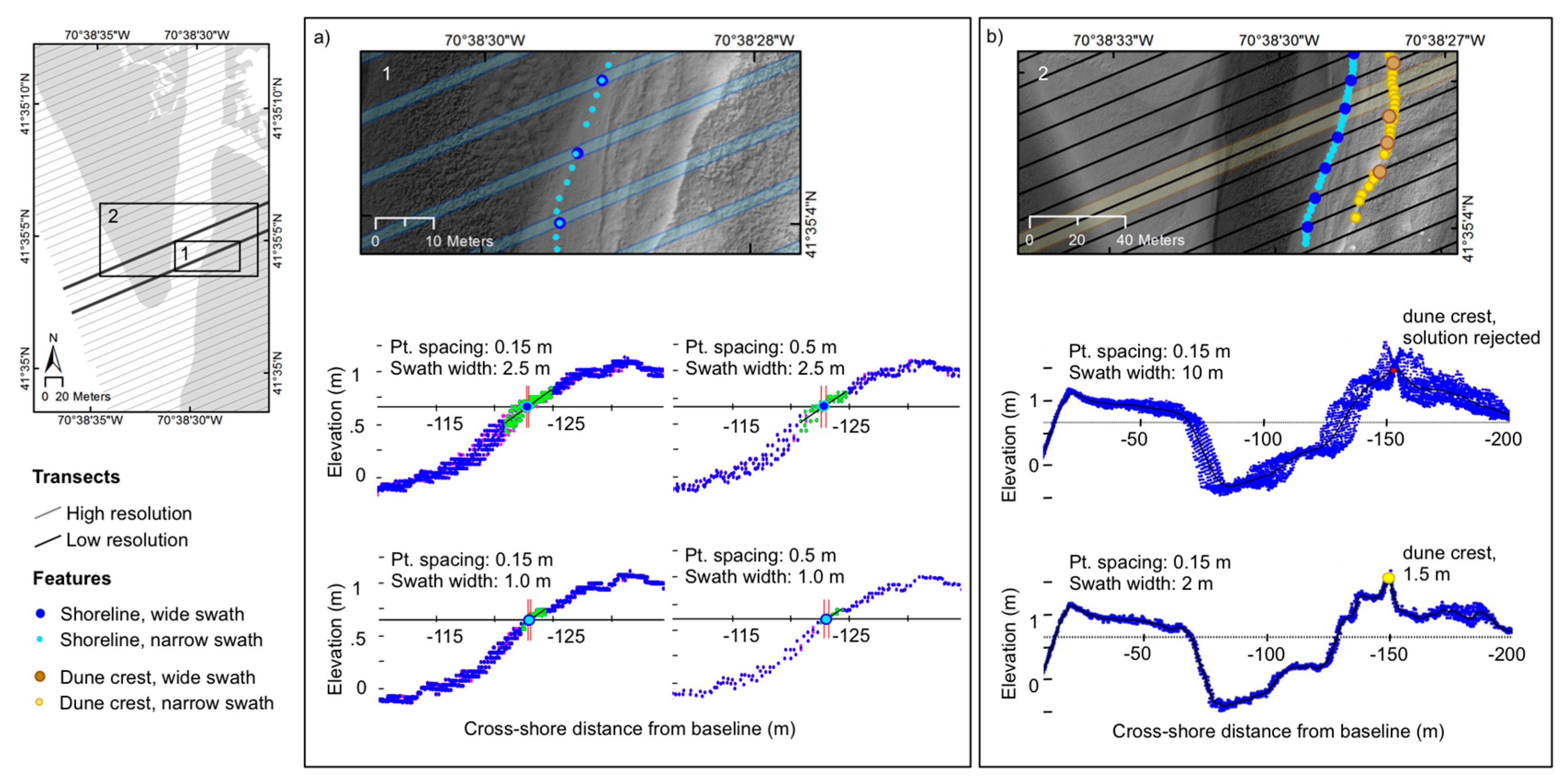
2.3.1. Geomorphic Feature Extraction

We used two feature extraction methods: one to extract shoreline position (similar to [21]) and the other to extract the positions of foredune toe and foredune crest [34]. Both methods have been broadly applied in U.S. coastal change assessments (e.g., [26]). Both methods were implemented in MATLAB (Release 2015b, Natick, MA, USA) and identify positions of the given features along cross-shore transects.
To evaluate the data densities required to extract geomorphic features, we decimated the 15-cm (low density) point cloud to 35 cm and 50 cm spacing. We used the Subsample tool in CloudCompare (v2.7, 2016, GPL software) to decimate the 15 cm point cloud by setting the minimum space between points to 35 and 50 cm in turn. From each of the three datasets (one dataset per point spacing), we performed two feature extractions: one using established processing parameters and the other with a narrowed swath width. This resulted in six products for each of the three feature types (shoreline, dune toe, and dune crest), enabling us to compare outputs of three point cloud densities and two sets of processing parameters.
To automatically detect shoreline position, MHW was located along a two-dimensional cross-shore elevation profile using a method similar to [21]. Onshore transects were cast perpendicular to a generalized offshore coastline at the designated transect spacing. All data points within 1 m (established parameter) or 0.5 m (narrowed width) of each transect were used in an automated process that (1) identified points on the foreshore; (2) fit a linear regression through these foreshore points; and (3) calculated where this regression line crossed the MHW elevation (z = 0.66 m). The intersection of the foreshore regression line with MHW was considered the geographic location of the shoreline. Each position that was visually identified as inaccurate when projected on its cross-shore profile was removed (e.g., Figure 4a). Positions were considered inaccurate when the detected point did not match the correct feature, such as a detected shoreline position that corresponded to a detached intertidal swash bar. These methods are commonly implemented with profiles spaced every 10 or 20 m (e.g., [21,34,35,36]). In this study, we maintained the 10-m transect spacing with the wider (2 m) swaths and we shortened the alongshore distance between transects to 2 m with the narrowed (1 m) swaths.
We extracted the three-dimensional position of the foredune toe and crest along cross-shore profiles using the methods developed by Stockdon et al. [34] (e.g., Figure 4b). Onshore transects were cast perpendicular to the coastline and a weighted average gridding routine was applied to the point cloud along each transect to produce cross-shore elevation profiles. As with the shoreline, we extracted foredune positions at two processing resolutions: grid cells of 2.5 m cross-shore by 10 m alongshore were considered low-resolution and cells of 1 m cross-shore by 2 m alongshore were considered high-resolution. The dune crest was defined as the peak of the most seaward dune within 200 m of the MHW shoreline. The dune toe was identified as the greatest point of inflection between the shoreline and the dune crest. The inflection point was required to be more than 0.5 m below the dune crest and have a negative surrounding curvature [34]. After the positions were extracted, the operator performed several rigorous quality control checks such as viewing all the features extracted for a beach system overlaid on the elevation data and using imagery as available [34]. If errors were identified, the operator manually viewed the cross-shore profile and either deleted or modified the position of the feature.

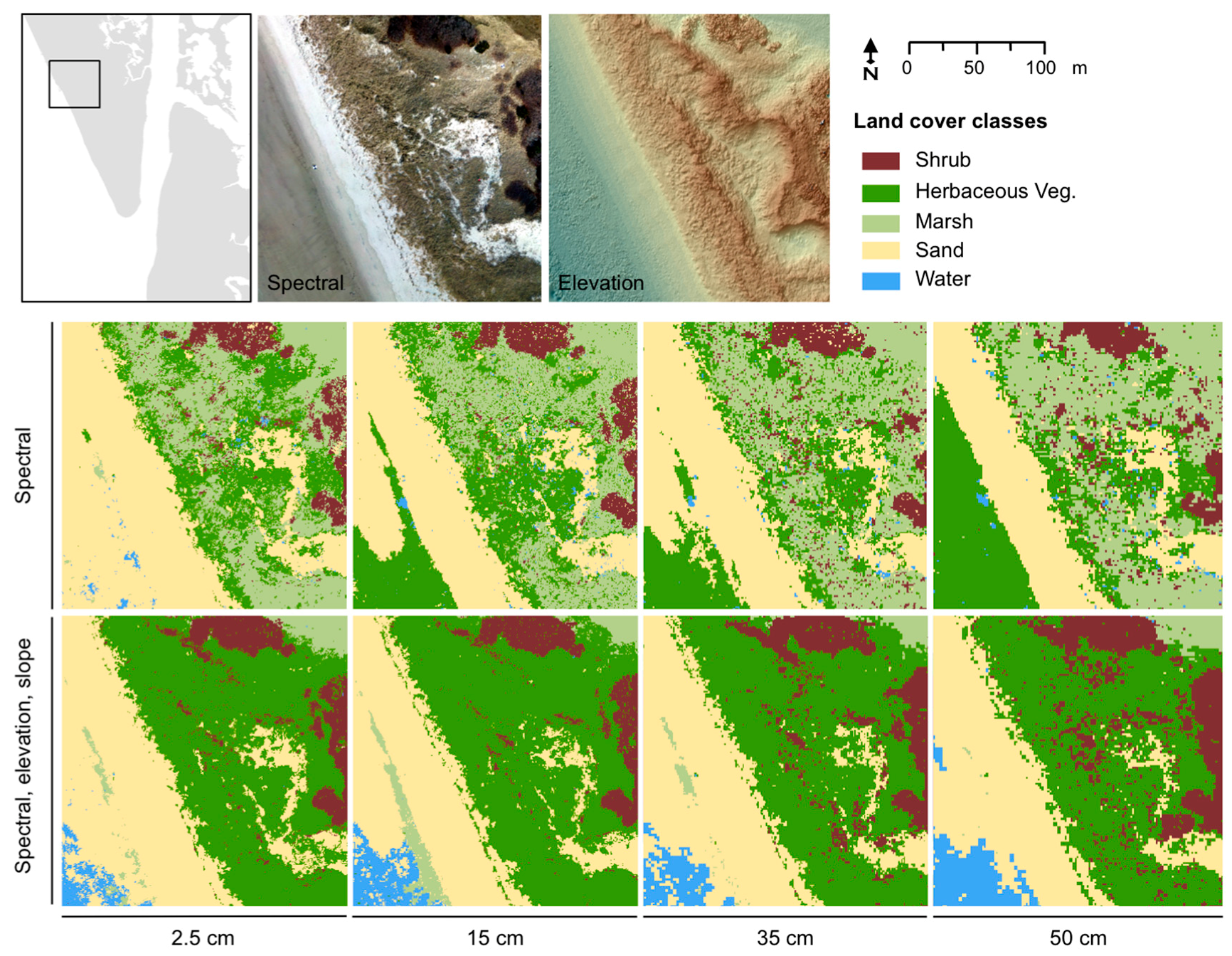
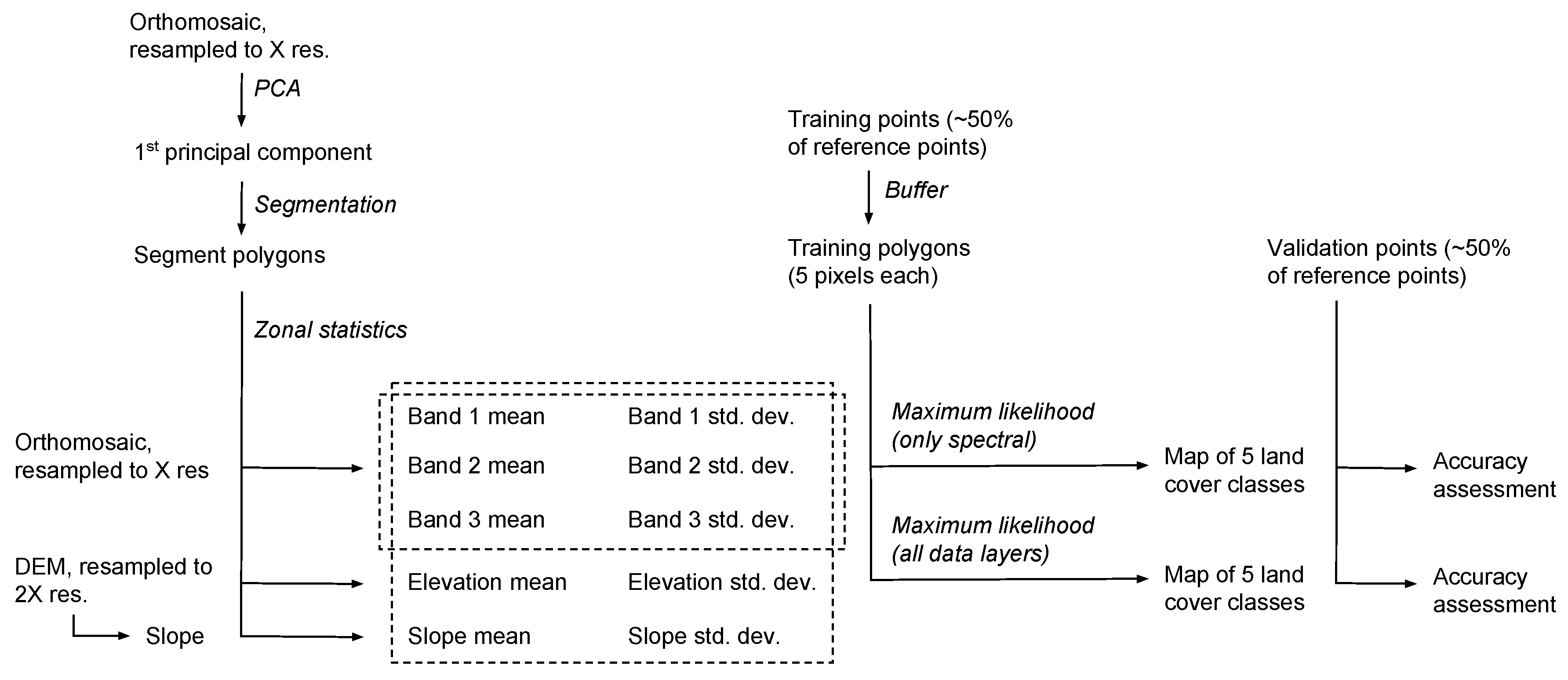
2.3.2. Land Cover Classification

Land cover was classified at four resolutions from two sets of input data using a supervised object-based maximum likelihood classification [37,38,39,40,41,42]. The workflow is diagrammed in Figure 5. Five land cover classes common to coastal habitat modeling (e.g., [43]) were used in the supervised classification including: water, sand, wetland vegetation (“marsh”), non-marsh herbaceous vegetation (“herbaceous vegetation”), and woody vegetation (“shrub”).
We measured the effect on accuracy of changes in two variables: the resolution of the input imagery and the incorporation of topographic data. The classification described below was performed for eight input dataset variations: (1–4) the orthomosaic (RGB bands) at four resolutions (2.5, 15, 35, and 50 cm) and (5–8) the orthomosaic at the same four resolutions with elevation and slope (ZSl) at twice the resolution of the imagery. The orthomosaic and the DEM were each resampled to the three downsampled resolutions using bilinear interpolation (Resample tool in ArcGIS v10.3, ESRI, Redlands, CA, USA). The resolutions of the elevation and slope datasets were proportionally scaled to the imagery datasets because the DEM produced by SfM was coarser than the orthomosaic by a factor of two. All classifications were performed with the same set of training and testing sites.
Land cover reference sites for training and validation were manually classified by reference to the imagery and elevation. We randomly distributed 500 points within the extent of the orthomosaic to initialize the reference dataset. This initial set was more than doubled by manually adding points (878 additional points) to create a representative sample of the land cover classes, in which the sample quantity in each class was roughly proportional to its coverage within the study area. A user familiar with the study site classified each point using a combination of site knowledge, landscape context, and visual clues in the orthomosaic and DEM. After classification, the reference points were randomly divided in two, to create a training dataset and a validation dataset. The set of 689 training points were used to train the classifier and the set of validation points was further supplemented with the same method described above, resulting in 726 validation points. The area represented by each training point was considered to include the five pixels with centroids nearest to the point, such that training samples represented 0.31 cm2 at 2.5 cm resolution, and 125 cm2 at 50 cm resolution.
Segmentation was performed in GRASS GIS (v7.0, Open Source Geospatial Foundation), on the first principal component of the three-band orthomosaic. The principal components analysis (PCA) was performed with the i.pca program in the image toolbox (“i.pca ‒n input=ortho_group output=ortho_pca”). At every resolution, the first component accounted for more than 95% of the variance in the scene, indicating that the other components contained substantial noise and redundancy. Using the i.segment program, contiguous pixels were grouped into segments if the degree of similarity was lower than the unit-less level 0.05 (similarity threshold = 0.05; no minimum size; “i.segment group=pc1 output=seg_pc1 threshold=0.05”). These segmentation parameters were optimized for all four input resolutions by (1) iteratively varying the parameters and visually assessing whether segments represented logical objects at each resolution and (2) by comparing the classifications resulting from the best-performing segmentation parameters.
The final segments at each resolution were used to aggregate each input information band before running a classification on the per segment mean and standard deviation rasters. To do so, we first vectorized the segments and converted them to ESRI shapefile format in GRASS, and then computed means and standard deviations per segment (Zonal Statistics tool in ArcGIS v10.3). Each input layer (i.e., each band of the orthomosaic, elevation and slope) produced two new object-based information layers: segment means and standard deviations. Maximum likelihood classification was run on the zonal rasters with the pre-defined training sites.

3. Results

To assess the utility of SfM photogrammetric processing for coastal change research, we examined: (1) the application of SfM to compute coastal elevation information [44]; (2) the extraction of shoreline, dune toe and dune crest from SfM-produced point clouds; and (3) the classification of land cover from SfM products for use in habitat mapping.

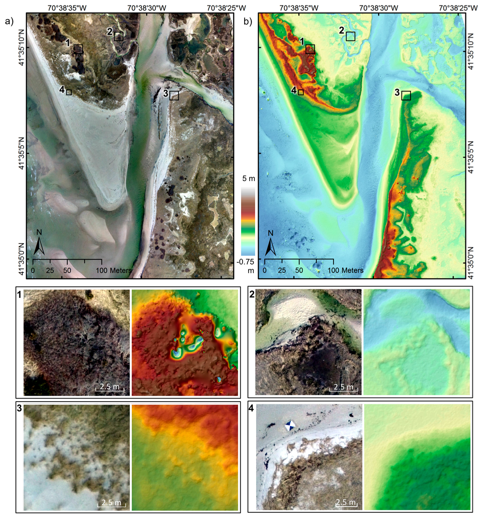
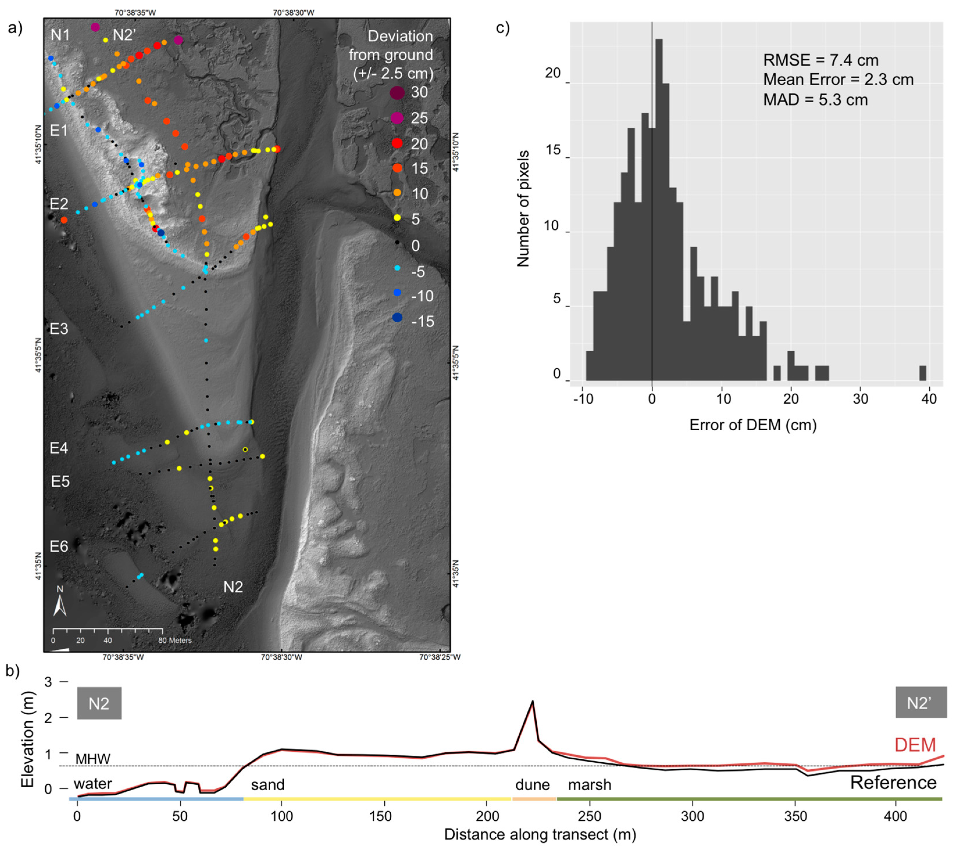
3.1. SfM Products: Elevation Surface Analysis

We estimated the point cloud error using a quadrature sum to combine error terms [45]. This method of quantifying error relied on comparison with the GCPs that were used to georeference the point cloud and derivative products. As such, these calculations were performed without external validation points. PhotoScan estimated the positional error of the GCP markers as 6 cm (root sum of squares (RSS) error of X, Y, and Z compared to surveyed positions of these points), considering a preset tie point accuracy value of 0.005 m. To fully capture the propagation of error among products, we calculated the quadrature sum of the errors estimated for (a) ground control (RTK GNSS) (1.7 cm), (b) reprojection (a measure of the precision of tie points; estimated at 1 cm), and (c) the final photogrammetric reconstruction calculated by PhotoScan (6 cm) [46]. This produced an error estimate of 6.7 cm, consisting of 6.1 cm horizontal error and 2.8 cm vertical error.
To determine an alternative, independent error metric, we compared a gridded elevation model built from the point cloud to the 254 reference points (Figure 6). At each reference point, we found the deviation of the DEM grid cell from the surveyed ground elevation. The DEM had a vertical root mean square error (RMSEZ) of 8.7 cm. In addition to the vertical error calculated for the DEM, we visually assessed differences in error along each transect (e.g., Figure 6b). The variation in error between transects appears related to the land cover that they traverse. The north–south transects (N1 and N2) sampled areas with the most varied terrain and the broadest extent of vegetation and had the greatest vertical error values. For example, the longest transect, N2 (RMSEZ of 7.7 cm), included areas of tidally-exposed sand, dry sand, dune with herbaceous vegetation, and marsh (Figure 6b).
The magnitude of error also varied with land cover type (Table 1). The greatest deviations from ground truth in the SfM elevation outputs occurred in areas with tall or dense vegetation. The classes with greatest RMSEZ in decreasing order were shrub (28.3 cm, only two reference points), marsh (12.8 cm), and herbaceous vegetation (6.2 cm). We also observed these land cover-based errors along the transects, such as along transect N2, where the DEM closely matched the reference elevations in the sand-covered southern half of the profile, but diverged from the reference elevations in the wetland-dominated northern half of the transect.

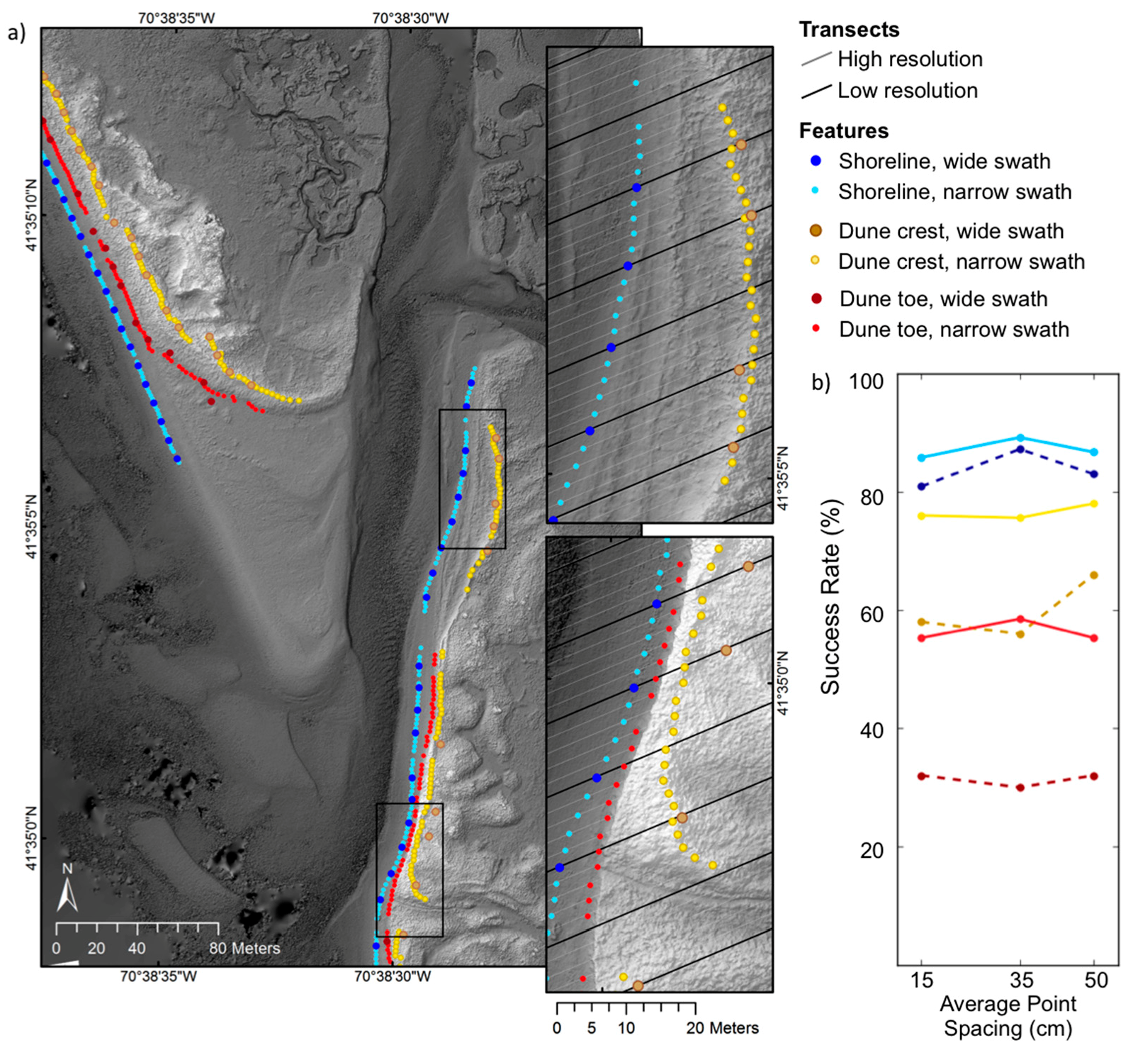
3.2. Geomorphic Feature Extraction

We assessed the utility of SfM for coastal change analyses by performing feature extraction processing in an experimental set-up using the different resolution datasets described above. Of the total number of transects evaluated, we calculated the percent of transects at which a feature position was successfully resolved (hereafter “success rate”). We compared the success rates of feature extraction from each dataset at each processing resolution and spatially displayed the resulting features to assess landscape patterns associated with extraction success or failure (Figure 7; Table 2).
There was a clear difference in success between the wide and narrow swath extractions: narrower swaths produced greater success rates than wider swaths (Figure 7). This difference was especially pronounced in the dune position extraction. When averaged for all point cloud spacing, dune positions were extracted with 21% greater success by narrow swaths (67%) than by wide swaths (46%). Extractions performed with wide swaths were particularly unfavorable for the extraction of dune toe positions. Dune toe extraction relied on successful dune crest extraction because it was positioned in relation to the dune crest.
Shoreline positions were resolved for 81–89% of the profiles across all shoreline extraction routines (both swath widths applied to all three point clouds) (Figure 7). The six sets of shoreline features had very little deviation from each other, which indicated consistent precision, although the shoreline positions extracted from more closely-spaced transects with narrower swaths represented greater alongshore variability without sacrificing success or precision. In contrast to the dunes, shoreline extraction was highly successful at both swath widths and all point cloud densities. These results were due in part to the lack of alongshore variability in the shoreline, which facilitated successful shoreline extraction.
We compared the solutions achieved at the 47 transects at which profiles were analyzed from both swath widths, and observed no consistent relationship between shoreline extraction and point cloud spacing (Figure 7; Table 2). The 2-m and 1-m swaths produced nearly identical shoreline positions at 35-cm spacing, with an 87% success rate. The change in swath width had a greater effect on the position solutions from the dune feature extraction in our comparison. Nineteen out of the 47 dune toes were detected only from the 2-m swath. Dune crest extraction from 10-m swaths exhibited the greatest variation across point clouds; the success rate produced for the 50-cm was about 10% greater than for the 15-cm and 35-cm point clouds.

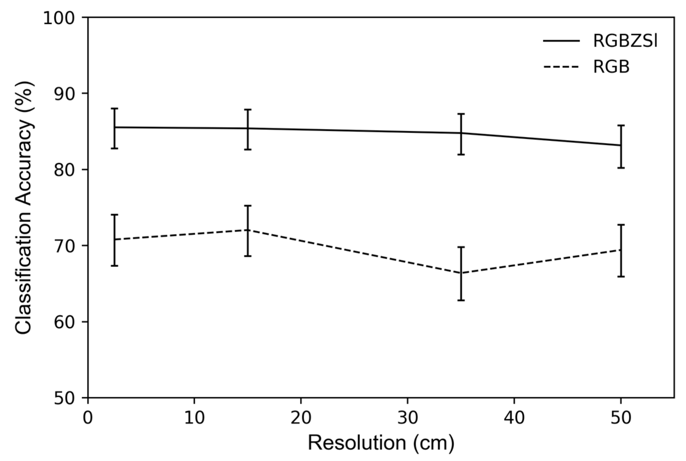
3.3. Land Cover Classification

We assessed the influence of resolution and incorporation of elevation on classification accuracy by comparing supervised image classification outcomes from SfM products and from downsampled datasets. The final classified images are presented in Figure 8; plots of overall accuracy for each classification are displayed in Figure 9; and tables of accuracy metrics are presented in Table 3. We compared the eight variations of input data by calculating both overall accuracy, which estimates the percent of accurately classified pixels out of the total, and the kappa coefficient, which attempts to account for chance agreement in its measure of classification success, (e.g., [47,48]). We assessed differences among land cover by comparing producer’s and user’s accuracy. Producer’s accuracy is the percent of the total pixels in a ground truth class that are classified correctly in the output image and user’s accuracy is the percent of all output image pixels in a given class that are classified correctly.
The resolution of the input layers had little effect on overall classification accuracy. There was greater variation in accuracy among the classifications performed with only spectral data, but that variation did not display any dependence on resolution (Figure 9). With the spectral classification, the greatest accuracy was achieved at 15-cm resolution and the lowest at 35-cm resolution.
The use of topographic data in the classification had a clear positive effect on accuracy. Classification performed with both topographic and visual reflectance data (12 information layers) produced highly accurate classified maps without significant differences in accuracy at resolutions finer than 50 cm (Figure 9, Table 3). The mean overall accuracy produced by RGB, elevation, and slope at the four resolutions was about 85% with a narrow range of values, whereas mean overall accuracy from spectral data was about 70% with a wider range. Improvements due to the inclusion of topographic data were especially evident in the herbaceous vegetation class. Herbaceous vegetation and marsh were the classes most difficult to distinguish without elevation information, as they are spectrally similar in optical data. Elevation information helped to differentiate herbaceous vegetation and marsh because of the intrinsic stratification of the land covers by topography (Figure 8).
The greatest accuracy gains by class were seen in marsh and non-marsh herbaceous vegetation classes (Table 3). With only spectral layers in the classification, 49% of the validation points classified as herbaceous vegetation were classified inaccurately and about half of those were actually marsh. When elevation and slope were included, about 80% of the herbaceous vegetation validation points were classified accurately. Marsh had the greatest representation within the validation sites. Without topography, 66% of them were allocated correctly, but with topography that increased to 88%.
We also observed reduced prevalence of the following errors when elevation and slope were included: sand misclassified as herbaceous; marsh misclassified as shrub; confusion between herbaceous vegetation and marsh; and very shallow water misclassified as herbaceous vegetation. The images classified with elevation showed greater spatial cohesion among classes, whereas the images classified without topography exhibit salt-and-pepper effect, in which neighboring pixels were incorrectly assigned to different classes (Figure 8). For all land cover classes, elevation in the classification improved the accuracy in every aspect, with the exception of user’s accuracy of the water class (Table 3). The fewest gains were seen in the sand and water classes, which were often confused during the classification. This is attributed to the lack of applying a water mask during either SfM or classification processing.

4. Discussion

4.1. UAS-SfM Elevation for Coastal Zones

Our results demonstrate that UAS-SfM is an excellent source of high-quality elevation data that compares favorably to lidar accuracy standards and is cost-effective and convenient to produce for appropriate spatial scales. Previous works have demonstrated the high quality of elevation data produced by UAS-SfM (e.g., [18,49,50,51,52]). We confirm these findings and build on the applicability of these datasets to coastal assessment.
Elevation point clouds of the coastal zone generated with UAS-SfM can be produced with less error and greater point density than published standards for airborne lidar. The most dense lidar product available for the coastal northeastern U.S. has 35 cm Nominal Point Spacing (NPS) and was compiled to meet RMSEZ of 5.2 cm for open terrain, which corresponds to the highest standard in the National Enhanced Elevation Assessment (NEEA), Quality Level 0 (QL0) [53,54]. The spacing of the Black Beach point cloud is more than six times denser than that dataset and has less vertical error than both that product and the mid-level lidar standard of quality (e.g., NEEA QL2) [53,55]. Producing these highly precise and highly accurate data required precise GNSS measurements and thorough distribution of georeference targets [50].
Unlike lidar, UAS-SfM using a passive sensor (camera) is unable to consistently produce bare-earth elevations in densely-vegetated areas [49,50]. The landscape of Black Beach included some dense vegetation, which resulted in the inclusion of vegetation effects in our SfM point cloud. More specifically, the SfM-derived elevations tended to exhibit a positive deviation from ground elevations in vegetated wetland areas, where the top of densely growing vegetation was measured instead of the ground surface recorded by GNSS surveying. However, in sand locations this effect was mitigated by lack of vegetation from the intertidal to foredune areas (Figure 6). For our specific analyses of geomorphic features and land cover, vegetation did not limit the quality of analysis. However, if project goals required bare earth elevations, techniques exist to mitigate canopy effects, such as using non-nadir imaging angles [56].
A novel advantage of SfM elevation datasets is that they are coincident with spectral data. This essentially doubles the amount of information of that offered by lidar datasets. These coincident datasets are especially advantageous in highly dynamic systems, such as coastal zones, where storms and recovery from storms often cause rapid changes to the landscape (i.e., hours, days, weeks). The UAS can be deployed rapidly for short-term measurements and SfM generates the elevation directly from the image products, meaning that perfect synchronization between the two is intrinsic. This synchronization is useful in many applications, such as the two explored here.

4.2. Geomorphic Feature Extraction

Our results demonstrate that established processing routines can be applied to UAS-SfM data to extract features consistent with existing geomorphic datasets for change monitoring and research. Profile-based feature extraction techniques have been applied to create consistent datasets of coastal change for uses such as vulnerability assessment and coastal modeling [34,57], which are dependent on the availability of elevation data with sufficient temporal resolution and data density to reflect current conditions. The profile-based shoreline position extraction technique employed here was originally designed for elevation point clouds produced by NASA ATM, which typically produced 15–20 elevation points suitable for use in analysis within a 2-m wide swath [21]. UAS-SfM datasets produce many more points in the profile, with great enough density that the potential for analysis is not realized by this method. Even after decimating the SfM point cloud, the decimated product was denser in the area of interest than the densest lidar available and had a more consistent distribution of points. If lidar data had been available for the same date, we infer that resolving the cross-shore profiles and confidently extracting feature positions might have been more successful from SfM point clouds than from lidar due to their consistent point spacing and density.
The chief advantage of SfM data for feature extraction is the increased precision of both the method and the resulting positions. Narrower swath widths were possible because of the high density of the SfM data; these narrower swaths resulted in more successful extraction overall and more precise feature positioning than from the wider swaths typically used. Furthermore, narrower swaths were particularly suitable for detecting features in variable coastal areas because the profiles had greater tolerance for small-scale alongshore variability than wider swath profiles. This tolerance was especially advantageous for resolving dune features, which tended to have greater variability than shoreline positions.

4.3. Land Cover Classification

High-quality elevation datasets can facilitate analyses of changing landscapes. Previous studies, which were performed at different scales and in different environments, suggested that elevation is a powerful variable in automated land cover classification [37,56,58]. However, it is uncommon to have high-resolution elevation data accompanying coastal imagery datasets. At this coastal site, we found that temporally coincident elevation and imagery improved the classification workflow; the synchronized SfM datasets facilitated manual training site classification and greatly improved automated image segmentation and supervised classification. The high-resolution of the imagery and the coincident elevation surface enabled the identification of contiguous features, which were used as the base units in object-based classification. In the supervised classification routine, the addition of elevation and slope data greatly improved classification accuracy whereas changes to the spatial resolution had minimal influence on accuracy. In temperate-latitude coastal areas such as Black Beach, topographic data are especially advantageous because land cover type is highly dependent on elevation. For example, sandy beaches with patches of coarse sediment tended to be found at low elevations at Black Beach, dune grass was more elevated, and isolated dwarf trees were easily distinguished in the DEM.
The classification was in part facilitated by the vegetation canopy effect because differences in elevation and slope helped to discriminate vegetation. The potential exists for combining elevation and classified vegetation surfaces to produce bare-earth elevations by identifying height offsets based on vegetation type. Canopy height models, such as those produced by [56] could improve the classification ability even further by allowing the characterization of more specific vegetation structure.

4.4. Advantages, Trade-Offs, and Limitations

Our study shows that the dual dataset of high-resolution imagery and elevation produced by UAS-SfM can be used for a variety of applications. Examples include confirmation of the positions of dynamic coastal features, particularly shorelines; derivation of features such as wet-dry lines with elevation information; masking water features; assisting in visual validation; and providing additional information during habitat classification routines, which we found dramatically increased land cover classification accuracy. We were able to use existing routines used in coastal change assessments to extract features from SfM data, which are therefore straightforward to incorporate to update coastal vulnerability assessments. More frequent surveys that provide time series measurements of storm response and recovery could be used to improve modeling and better resolve coastal processes and the relative influence of drivers of change in a given area. Furthermore, UAS could enhance models of coastal change through temporally frequent surveys to capture short-term changes related to storm impact and recovery, similar to previous work using stereophotogrammetry and lidar for change assessments [8]. Although the datasets are highly accurate and precise, using them for change assessment will require rigorous calibration between the datasets, such as those performed for lidar data [8,52].
Differences in imagery resolution have distinct trade-offs that are important to consider when planning future work. Although we were able to produce results at several resolutions, we found few gains are provided by dataset resolution finer than 35 cm (both point spacing and pixel size). The classification quality was not degraded at lower image resolutions (≤50 cm); therefore, it appears that higher altitude surveys that provide greater spatial coverage and lower resolutions could be flown without affecting results negatively. The principal advantage of the 2.5 cm resolution imagery in this survey was a minimized need for time-intensive in situ reference surveying. For example, we were able to confidently identify small sand pits among the dunes that might otherwise have required additional in situ labor to distinguish the sand from the surrounding dry grass. Expanding upon the goals of this project, high-resolution imagery could be used to visually identify parameters important for habitat suitability, such as species use of an area and the associated sediment grain size. Thus, an opportunity exists to optimize resolution to meet scientific goals by identifying the smallest object that should be distinguishable in the imagery.
In addition to the advantages described above, data collection with UAS presents limitations. In addition to the dependence on suitable meteorological conditions [19,59], coverage is limited, particularly when compared with the extents available through manned aircraft platforms, making UAS better suited to small-scale and high-resolution projects. However, as this study demonstrates, such high-resolution studies can provide valuable information on trade-offs in study design and aid in the selection of appropriate platforms and resolution.
The accuracy of the photogrammetric product described here currently relies on thoroughly distributed and highly accurate ground control, although we expect this to be mitigated with increased precision of onboard UAS GNSS devices. UAS operations are also somewhat limited by environmental conditions, requiring low wind levels (in this case <10 m/s), dry conditions, and adequate lighting. Furthermore, this project did not encounter some of the UAS deployment limitations that might be expected for coastal areas, such as study site accessibility or a dense population of humans or other organisms (e.g., flocks of resting or roosting birds) using the beach that would introduce error and uncertainty in the elevations and classifications.
Despite these limitations, our assessment shows that products generated with these datasets can be integrated with existing workflows to expand records of coastal features and to enhance research into coastal vulnerability. With more immediate, flexible, and less resource-intensive deployment than established technologies for measuring coastal change, UAS-SfM is well-suited for repeat surveys to assess spatial and temporal changes at small spatial extents and to better understand how these may be linked with site-specific processes along the coast.

5. Conclusions

SfM applied to low-altitude aerial imagery such as that collected by UAS provides highly accurate visual reflectance and topographic data with elevation precision only slightly degraded from survey-grade RTK GNSS, better than typical airborne lidar and covering a continuous area. We show that SfM products can be used to derive datasets of geomorphic features and classified land cover consistent with publicly available elevation and imagery datasets. These techniques enable extraction of geomorphic features at higher resolutions and with greater precision than previously possible. They improve land cover classification accuracy by adding coincident elevation data to the image analysis. We find that data densities greater than 35 cm resolution do not contribute to improved processing or product accuracy with these techniques.
UAS surveys can be processed similarly to lidar and other aerial or satellite surveys for coastal research assessments, but with more immediate, flexible, and less resource-intensive deployment. UAS-SfM imagery and derived topographic data are available at considerably higher resolutions and spatial point densities than other surveying methods, resulting in higher precision of both derived products and extracted features, particularly in sandy beach areas. The capability for rapid deployment, survey collection, and data processing makes UAS an optimal survey tool to conduct repeat surveys over areas of limited spatial coverage, and can be coupled with other types of data to improve our understanding of process-based coastal change over timescales of days, weeks, seasons, and years.

Acknowledgments

This project was funded by the U.S. Geological Survey (USGS) Coastal and Marine Geology Program and the Department of the Interior Northeast Climate Science Center. Sawyer Stippa developed much of the initial UAS processing steps and workflow. We thank Jon Warrick of the USGS for a thoughtful review of a draft manuscript. We thank the four anonymous journal reviewers for their insight and suggestions that improved the manuscript. Any use of trade, firm, or product names is for descriptive purposes only and does not imply endorsement by the U.S. Government.

Author Contributions

Emily J. Sturdivant designed and performed the analysis and wrote the manuscript. E. Robert Thieler and Erika E. Lentz conceived the project, secured funding, and assisted in writing the manuscript. Amy S. Farris and Kathryn M. Weber performed the geomorphic feature extraction. David P. Remsen and Simon Miner provided UAS resources and conducted the UAS operation. Rachel E. Henderson provided photogrammetry technical expertise.

Conflicts of Interest

The authors declare no conflict of interest. The founding sponsors had no role in the design of the study; in the collection, analyses, or interpretation of data; in the writing of the manuscript, and in the decision to publish the results.

Appendix A

Table A1. Parameters used during SfM processing to create the dense point cloud.
Process StepProcess DescriptionPhotoScan Tools and ParametersOutput Properties
Add photosLoaded all 250 cameras with high (>0.5 estimated) quality.
Convert camera coordinates to projected coordinate system.
Define camera location accuracy.
“Estimate Image Quality”
“Convert”
To: NAD83 UTM Zone 19N
Reference Settings:
Camera accuracy (m): 10
Range of image quality: 0.69–1.26
Import GCPsAssociated ground coordinates with GCP targets visible in images.
Manually checked the placement of each GCP in the image.
“Detect markers”
Tolerance: 50%
Labeled each GCP in text file to correspond to the name of the marker in PhotoScan.
“Import Markers…” to load GCP text file
Northing: Local_N
Easting: Local_E
Altitude: Local_Z
Display all the images with a GCP present and adjust the position of the marker if necessary.
Reference Settings:
Tie point accuracy (m): 0.005
Align photosGenerated sparse point cloud of tie points between photos.“Align Photos”
Accuracy: High
Pair preselection: Reference
Key point limit: 5000
Tie point limit: 0
Aligned 211 photos
Optimize camera calibration 1Iteratively eliminated tie points to achieve an optimal error estimate.
Optimized cameras after deleting set of points.
Selected points based on several criteria of accuracy.
“Gradual selection”
Reconstruction uncertainty: Level 10
Projection accuracy: Level 9
Projection accuracy: Level 6
Reprojection error: Level 0.5 (~10% of remaining points)
Manually delete points that are obviously removed from the general surface.
Initial marker error: 0.62 m
Initial marker error: 0.58 pix
Final marker error: 0.05 m
Final marker error: 0.366 pix
Dense point cloudRotated and resized the region.
Built the dense point cloud.
Rotate and resize the region to be generally orthogonal to lines of latitude and to limit the extent to just outside of the area with GCPs.
“Build Dense Cloud”
Quality: High
Depth filtering: Mild
67,885,040 points in the dense point cloud.
Refine the point cloudManually deleted points that are obviously separate from the surface.Rotate the point cloud to view from the side and manually delete chunks of points that are isolated from the surface.
Generate outputsExported a point cloud for shoreline extraction.
Exported a DEM.
Exported an orthomosaic.
“Build DEM”
Source data: Dense Cloud
Interpolation: Enabled
“Build Orthomosaic”
Type: Geographic
Surface: DEM
Blending mode: Mosaic
DEM resolution: 4.95 cm
1 Iterations were performed with the following target values: reconstruction uncertainty: 10; projection accuracy: 3; reprojection error: 0.3 pixels. If approximately more than 20% of the points were flagged at the target value, the threshold was adjusted to select only about 10% of the points.

References

  1. Morton, R.A.; Leach, M.P.; Paine, J.G.; Cardoza, M.A. Monitoring Beach Changes Using GPS Surveying Techniques. J. Coast. Res. 1993, 9, 702–720. [Google Scholar]
  2. Stockdon, H.F.; Doran, K.S.; Sallenger, A.H.; Beach, W.P. Extraction of Lidar-Based Dune-Crest Elevations for Use in Examining the Vulnerability of Beaches to Inundation During Hurricanes. J. Coast. Res. 2009, SI, 59–65. [Google Scholar] [CrossRef]
  3. Thieler, E.R.; Danforth, W.W. Historical shoreline mapping (II): Application of the digital shoreline mapping and analysis systems (DSMS/DSAS) to shoreline change mapping in Puerto Rico. J. Coast. Res. 1994, 10, 600–620. [Google Scholar]
  4. Schwab, W.C.; Thieler, E.R.; Allen, J.R.; Foster, D.S.; Ann, B.; Denny, J.F.; Spring, F.; Inlet, S.; Island, L.; York, N.; et al. Influence of Inner-Continental Shelf Geologic Framework on the Evolution and Behavior of the Barrier-Island System Between Fire Island Inlet and Shinnecock Inlet, Long Island, New York. J. Coast. Res. 2000, 16, 408–422. [Google Scholar]
  5. McNinch, J.E. Geologic control in the nearshore: Shore-oblique sandbars and shoreline erosional hotspots, Mid-Atlantic Bight, USA. Mar. Geol. 2004, 211, 121–141. [Google Scholar] [CrossRef]
  6. Harris, M.S.; Gayes, P.T.; Kindinger, J.L.; Flocks, J.G.; Krantz, D.E.; Donovan, P. Quaternary Geomorphology and Modern Coastal Development in Response to an Inherent Geologic Framework: An Example from Charleston, South Carolina. J. Coast. Res. 2005, 211, 49–64. [Google Scholar] [CrossRef]
  7. Aagaard, T.; Davidson-Arnott, R.; Greenwood, B.; Nielsen, J. Sediment supply from shoreface to dunes: Linking sediment transport measurements and long-term morphological evolution. Geomorphology 2004, 60, 205–224. [Google Scholar] [CrossRef]
  8. Lentz, E.E.; Hapke, C.J.; Stockdon, H.F.; Hehre, R.E. Improving understanding of near-term barrier island evolution through multi-decadal assessment of morphologic change. Mar. Geol. 2013, 337, 125–139. [Google Scholar] [CrossRef]
  9. Hapke, C.J.; Kratzmann, M.G.; Himmelstoss, E.A. Geomorphic and human influence on large-scale coastal change. Geomorphology 2013, 199, 160–170. [Google Scholar] [CrossRef]
  10. Jin, S.; Yang, L.; Danielson, P.; Homer, C.; Fry, J.; Xian, G. A comprehensive change detection method for updating the National Land Cover Database to circa 2011. Remote Sens. Environ. 2013, 132, 159–175. [Google Scholar] [CrossRef]
  11. Burger, J. Physical and social determinants of nest-site selection in Piping Plover in New Jersey. Condor 1987, 89, 811–818. [Google Scholar] [CrossRef]
  12. Sallenger, A.H.; Krabill, W.B.; Swift, R.N.; Brock, J.C.; List, J.H.; Hansen, M.; Holman, R.A.; Manizade, S.; Sontag, J.; Meredith, A.; et al. Evaluation of airborne topographic lidar for quantifying beach changes. J. Coast. Res. 2003, 19, 125–133. [Google Scholar]
  13. Ruggiero, P.; Kaminsky, G.M.; Gelfenbaum, G.; Voigt, B. Seasonal to Interannual Morphodynamics along a High-Energy Dissipative Littoral Cell. J. Coast. Res. 2005, 21, 553–578. [Google Scholar] [CrossRef]
  14. FitzGerald, D.M.; Fenster, M.S.; Argow, B.A.; Buynevich, I.V. Coastal Impacts Due to Sea-Level Rise. Annu. Rev. Earth Planet. Sci. 2008, 36, 601–647. [Google Scholar] [CrossRef]
  15. Mason, D.C.; Gurney, C.; Kennett, M. Beach Topography Mapping: A Comparison of Techniques. J. Coast. Conserv. 2000, 6, 113–124. [Google Scholar] [CrossRef]
  16. Young, A.P.; Ashford, S.A. Application of Airborne LIDAR for Seacliff Volumetric Change and Beach-Sediment Budget Contributions. J. Coast. Res. 2006, 22, 307–318. [Google Scholar] [CrossRef]
  17. Anderson, K.; Gaston, K.J. Lightweight unmanned aerial vehicles will revolutionize spatial ecology. Front. Ecol. Environ. 2013, 11, 138–146. [Google Scholar] [CrossRef]
  18. Harley, M.D.; Turner, I.L.; Short, A.D.; Ranasinghe, R. Assessment and integration of conventional, RTK-GPS and image-derived beach survey methods for daily to decadal coastal monitoring. Coast. Eng. 2011, 58, 194–205. [Google Scholar] [CrossRef]
  19. Casella, E.; Rovere, A.; Pedroncini, A.; Stark, C.P.; Casella, M.; Ferrari, M.; Firpo, M. Drones as tools for monitoring beach topography changes in the Ligurian Sea (NW Mediterranean). Geo-Mar. Lett. 2016, 1–13. [Google Scholar] [CrossRef]
  20. Sturdivant, E.J.; Lentz, E.E.; Thieler, E.R.; Remsen, D.P.; Miner, S. Topographic, Imagery, and Raw Data Associated with Unmanned Aerial Systems (UAS) Flights over Black Beach, Falmouth, Massachusetts on 18 March 2016; U.S. Geological Survey: Reston, VA, USA, 2017. [CrossRef]
  21. Stockdon, H.F.; Sallenger, A.H., Jr.; List, J.H.; Holman, R.A. Estimation of Shoreline Position and Change Using Airborne Topographic Lidar Data. J. Coast. Res. 2002, 18, 502–513. [Google Scholar]
  22. Sallenger, A.H. Storm Impact Scale for Barrier Islands. J. Coast. Res. 2000, 16, 890–895. [Google Scholar]
  23. Yang, Z.; Myers, E.P.; Jeong, I.; White, S.A. VDatum for the Gulf of Maine: Tidal Datums and the Topography of the Sea Surface. In Technical Memorandum NOS CS 31; National Oceanic and Atmospheric Administration: Silver Spring, MD, USA, 2013. [Google Scholar]
  24. Hartman, J.; Caswell, H.; Valiela, I. Effects of wrack accumulation on salt marsh vegetation. Oceanol. Acta 1983, (Special issue (0399-1784)), 99–102. Available online: http://archimer.ifremer.fr/doc/00247/35784 (accessed on 27 September 2017).
  25. Valiela, I.; Teal, J.M. The nitrogen budget of a salt marsh ecosystem. Nature 1979, 280, 652–656. [Google Scholar] [CrossRef]
  26. Hapke, C.J.; Himmelstoss, E.A.; Kratzmann, M.G.; List, J.H.; Thieler, E.R. National Assessment of Shoreline Change: Historical Shoreline Change along the New England and Mid-Atlantic Coasts. In Open-File Report 2010-1118; U.S. Geological Survey: Reston, VA, USA, 2011; p. 57. [Google Scholar]
  27. Thieler, E.R.; Smith, T.L.; Knisel, J.M.; Sampson, D.W. Massachusetts Shoreline Change Mapping and Analysis Project, 2013 Update. In Technical Report 2012–1189; U.S. Geological Survey: Reston, VA, USA, 2013. [Google Scholar]
  28. Tucker, J.; Barker, B.; Geyer, R.; Muramoto, J.A.; Schwarzman, B.; Taylor, D.; Thieler, R.; Weidman, C. The Future of Falmouth’s Buzzards Bay Shore: Report of the Coastal Resources Working Group to the Board of Selectmen, Falmouth, Massachusetts. Available online: http://www.falmouthmass.us/documentcenter/view/4005 (accessed on 27 September 2017).
  29. Massachusetts Natural Heritage & Endangered Species Program. Summary of the 2016 Massachusetts Piping Plover Census; Natural Heritage and Endangered Species Program & Endangered Species Program Massachusetts Division of Fisheries & Wildlife: Westborough, MA, USA, 2016.
  30. Lucieer, A.; de Jong, S.M.; Turner, D. Mapping landslide displacements using Structure from Motion (SfM) and image correlation of multi-temporal UAV photography. Prog. Phys. Geogr. 2014, 38, 97–116. [Google Scholar] [CrossRef]
  31. Warrick, J.A.; Ritchie, A.C.; Adelman, G.; Adelman, K.; Limber, P.W. New Techniques to Measure Cliff Change from Historical Oblique Aerial Photographs and Structure-from-Motion Photogrammetry. J. Coast. Res. 2016, 32. [Google Scholar] [CrossRef]
  32. Agisoft PhotoScan. Agisoft Community Forum. Available online: http://www.agisoft.com/forum/index.php?topic=1970.0 (accessed on 27 September 2017).
  33. Agisoft. Agisoft Photoscan User Manual: Professional Edition; Agisoft LLC: St. Petersburg, Russia, 2015. [Google Scholar]
  34. Stockdon, H.F.; Doran, K.J.; Thompson, D.M.; Sopkin, K.L.; Plant, N.G. National Assessment of Hurricane-Induced Coastal Erosion Hazards: Gulf of Mexico; U.S. Geological Survey: Reston, VA, USA, 2012.
  35. Plant, N.G.; Holland, K.T.; Puleo, J.A. Analysis of the scale of errors in nearshore bathymetric data. Mar. Geol. 2002, 191, 71–86. [Google Scholar] [CrossRef]
  36. Hapke, C.J.; Reid, D.; Richmond, B.M.; Ruggiero, P.; List, J. National Assessment of Shoreline Change, Part 3: Historical Shoreline Change and Associated Coastal Land Loss along Sandy Shorelines of the California Coast; U.S. Geological Survey: Reston, VA, USA, 2006.
  37. Syed, S.; Dare, P.; Jones, S. Automatic classification of land cover features with high resolution imagery and LIDAR data: An object-oriented approach. In Proceedings of the SSC2005 Spatial Intelligence, Innovation and Praxis: The National Biennial Conference of the Spatial Sciences Institut, Los Angeles, CA, USA, September 2005; Spatial Sciences Institute: Los Angeles, CA, USA, 2005; pp. 512–522. [Google Scholar]
  38. Moran, E.F. Land Cover Classification in a Complex Urban-Rural Landscape with Quickbird Imagery. Photogramm. Eng. Remote Sens. 2010, 76, 159–1168. [Google Scholar]
  39. Myint, S.W.; Gober, P.; Brazel, A.; Grossman-Clarke, S.; Weng, Q. Per-pixel vs. object-based classification of urban land cover extraction using high spatial resolution imagery. Remote Sens. Environ. 2011, 115, 1145–1161. [Google Scholar] [CrossRef]
  40. Laliberte, A.S.; Rango, A. Texture and scale in object-based analysis of subdecimeter resolution unmanned aerial vehicle (UAV) imagery. IEEE Trans. Geosci. Remote Sens. 2009, 47, 1–10. [Google Scholar] [CrossRef]
  41. Laliberte, A.S.; Rango, A. Image Processing and Classification Procedures for Analysis of Sub-decimeter Imagery Acquired with an Unmanned Aircraft over Arid Rangelands. GIScience Remote Sens. 2011, 48, 4–23. [Google Scholar] [CrossRef]
  42. Ventura, D.; Bruno, M.; Jona Lasinio, G.; Belluscio, A.; Ardizzone, G. A low-cost drone based application for identifying and mapping of coastal fish nursery grounds. Estuari. Coast. Shelf Sci. 2016, 171, 85–98. [Google Scholar] [CrossRef]
  43. Gieder, K.D.; Karpanty, S.M.; Fraser, J.D.; Catlin, D.H.; Gutierrez, B.T.; Plant, N.G.; Turecek, A.M.; Robert Thieler, E. A Bayesian network approach to predicting nest presence of the federally-threatened piping plover (Charadrius melodus) using barrier island features. Ecol. Model. 2014, 276, 38–50. [Google Scholar] [CrossRef]
  44. Mancini, F.; Dubbini, M.; Gattelli, M.; Stecchi, F.; Fabbri, S.; Gabbianelli, G. Using unmanned aerial vehicles (UAV) for high-resolution reconstruction of topography: The structure from motion approach on coastal environments. Remote Sens. 2013, 5, 6880–6898. [Google Scholar] [CrossRef] [Green Version]
  45. Sherwood, C.R. Point Cloud from Low-Altitude Aerial Imagery from Unmanned Aerial System (UAS) Flights over Coast Guard Beach, Nauset Spit, Nauset Inlet, and Nauset Marsh, Cape Cod National Seashore, Eastham, Massachusetts on 1 March 2016 (LAZ file); U.S. Geological Survey: Reston, VA, USA, 2017.
  46. Hehre, R.E.; Hapke, C.J. Development of Historical Topographic Models of the Beach/Dune System in Northeast Coastal and Barrier Network Parks: Progress 13 August 2008. Technical Report March, 2010. Available online: https://irma.nps.gov/DataStore/Reference/Profile/2239454 (accessed on 27 September 2017).
  47. Congalton, R.G. A review of assessing the accuracy of classification of remotely sensed data. Remote Sens. Environ. 1991, 37, 34–46. [Google Scholar] [CrossRef]
  48. Foody, G.M. Status of land cover classification accuracy assessment. Remote Sens. Environ. 2002, 80, 185–201. [Google Scholar] [CrossRef]
  49. Westoby, M.J.; Brasington, J.; Glasser, N.F.; Hambrey, M.J.; Reynolds, J.M. ‘Structure-from-Motion’ photogrammetry: A low-cost, effective tool for geoscience applications. Geomorphology 2012, 179, 300–314. [Google Scholar] [CrossRef] [Green Version]
  50. Smith, M.W.; Carrivick, J.L.; Quincey, D.J. Structure from motion photogrammetry in physical geography. Prog. Phys. Geogr. 2015, 40. [Google Scholar] [CrossRef]
  51. Hugenholtz, C.H.; Whitehead, K.; Brown, O.W.; Barchyn, T.E.; Moorman, B.J.; LeClair, A.; Riddell, K.; Hamilton, T. Geomorphological mapping with a small unmanned aircraft system (sUAS): Feature detection and accuracy assessment of a photogrammetrically-derived digital terrain model. Geomorphology 2013, 194, 16–24. [Google Scholar] [CrossRef]
  52. Mitasova, H.; Overton, M.F.; Recalde, J.J.; Bernstein, D.J.; Freeman, C.W. Raster-Based Analysis of Coastal Terrain Dynamics from Multitemporal Lidar Data. J. Coast. Res. 2009, 252, 507–514. [Google Scholar] [CrossRef]
  53. Heidemann, H.K. Lidar Base Specification (ver. 1.2); U.S. Geological Survey: Reston, VA, USA, 2014; p. 41.
  54. NOAA National Ocean Service. 2013–2014 U.S. Geological Survey CMGP LiDAR: Post Sandy (MA, NH, RI); National Oceanic and Atmospheric Administration: Silver Springs, MD, USA, 2015.
  55. Abdullah, Q.; Maune, D.; Smith, D.; Heidemann, H.K. ASPRS Positional Accuracy Standards for Digital Geospatial Data. Photogramm. Eng. Remote Sens. 2015, 81, 1–26. [Google Scholar]
  56. Cunliffe, A.M.; Brazier, R.E.; Anderson, K. Ultrafine grain landscape-scale quantification of dryland vegetation structure with drone-acquired structure-from-motion photogrammetry. Remote Sens. Environ. 2016, 183, 129–143. [Google Scholar] [CrossRef] [Green Version]
  57. Gutierrez, B.T.; Plant, N.G.; Thieler, E.R.; Turecek, A.M. Using a Bayesian network to predict barrier island geomorphologic characteristics. J. Geophys. Res. Earth Surf. 2015, 120, 2452–2475. [Google Scholar] [CrossRef]
  58. Rogan, J.; Miller, J.; Stow, D.; Franklin, J.; Levien, L.; Fischer, C. Land-cover change monitoring with classification trees using Landsat TM and ancillary data. Photogramm. Eng. Remote Sens. 2003, 69, 793–804. [Google Scholar] [CrossRef]
  59. Gonçalves, J.A.; Henriques, R. UAV Photogrammetry for Topographic Monitoring of Coastal Areas. ISPRS J. Photogramm. Remote Sens. 2015, 104, 101–111. [Google Scholar] [CrossRef]
Figure 1. Workflow implemented in the project.
Remotesensing 09 01020 g001
Figure 2. Local context of study area in (a) Massachusetts (black square) and (b) along the Buzzards Bay coast displayed with aerial imagery acquired in summer 2013 (2013 Massachusetts DEP Natural Color Imagery collected for NOAA, NOS, OCM between 28 May 2013 and 9 September 2013). (c) Map of the survey at Black Beach, MA: black and white squares indicate the locations of targets used as ground control points (GCPs); black dots represent 254 independent reference points; the orange line represents the path flown at approximately 35 m altitude by the UAS (not including take off and landing sequences); and white squares within the flight path represent the location of the camera at the time of capturing each photograph.
Remotesensing 09 01020 g002
Figure 3. Raster surfaces produced from low-altitude aerial images using Structure-from-Motion (SfM): (a) orthomosaic image and (b) digital elevation model (DEM) displayed with hillshading. Inset maps demonstrate the degree to which landscape features are resolved in these products.
Remotesensing 09 01020 g003
Figure 4. Examples of feature extraction using cross-shore elevation profiles. (a) Shoreline extraction at the transect represented by the blue swath in the center of the map (Inset 1). Shoreline positions are represented in the map and the cross-shore elevation plots as blue points; dark blue points were positioned from the wide swaths and light blue points were positioned from the narrow swaths. Green points represent the foreshore region with a black line representing a linear regression fit through those points; red vertical lines indicate the 95% confidence interval of the solution. The four plots show profiles extracted in 2-m and 1-m alongshore swaths from the 15-cm and 50-cm spaced point cloud (as indicated). (b) Dune feature extraction at the transect represented by the yellow band in the map (Inset 2) from 15-cm spaced point clouds and at two swath widths, as indicated. A yellow point represents a dune crest that was extracted successfully; a red point represents a solution rejected by the operator. Dune toe position could not be computed in either profile and dune crest position was only identified with the 2-m swath.
Remotesensing 09 01020 g004
Figure 5. Workflow used for land cover classification. The process was performed four times, with X equal to 2.5 cm, 15 cm, 35 cm, and 50 cm.
Remotesensing 09 01020 g005
Figure 6. Deviation of DEM elevation from GNSS-surveyed reference elevations. (a) Reference points displayed on the DEM and symbolized by DEM deviation: small black points indicate an absolute deviation of less than 2.5 cm; blue and larger points represent increasingly negative deviation (where DEM measured lower elevation than reference); warm colors and larger points represent increasingly positive deviation (where DEM measured higher elevation than reference). (b) Elevation (m) along Transect N2 measured at reference points (black) and by the SfM DEM (red). The vertical root mean square error (RMSEZ) for Transect N2 is 7.7 cm. (c) Histogram of DEM deviations from reference elevations; bin width is 1 cm and the black vertical line indicates no deviation.
Remotesensing 09 01020 g006
Figure 7. Feature positions extracted from two swath widths. (a) Map of geomorphic feature positions calculated from the 35-cm spaced UAS-SfM point cloud. Blue points represent shoreline; red represent dune toe; and yellow represent dune crest. (b) Success rate (percent of transects at which a feature was successfully solved) of shoreline, dune toe, and dune crest extraction from wide and narrow swaths (dotted and solid lines, respectively) plotted against average point spacing of the input point cloud.
Remotesensing 09 01020 g007
Figure 8. Example area of land cover maps of Black Beach classified from RGB with and without topographic data at four resolutions.
Remotesensing 09 01020 g008
Figure 9. Overall classification accuracy plotted against input imagery resolution for classifications using visual (RGB; dashed line) and visual and topographic (RGBZSl; solid line) data. Vertical bars indicate 95% confidence interval. Note that y-axis values begin at 50.
Remotesensing 09 01020 g009
Table 1. Vertical accuracy by land cover presented as mean error, mean absolute deviation (MAD), and RMSEZ. Points were classified from the final 15-cm thematic map and manually verified. “Marsh” includes wetland vegetation; “Herbaceous Vegetation” includes non-marsh herbaceous vegetation; and “Shrub” includes woody vegetation.
Land CoverNMean Error (cm)MAD (cm)RMSEZ (cm)
Herbaceous Vegetation761.14.96.2
Marsh4611.611.612.8
Sand102−1.62.93.6
1 Shrub223.823.828.3
Water242.93.24.3
1 Two samples were used for calculations in the shrub class.
Table 2. Success rate of shoreline, dune toe, and dune crest by high- and low-resolution processing as extracted from the same point cloud with point spacing of 15, 35, and 50 cm. Success rate is the percent of transects at which a feature was successfully resolved.
Feature TypeSwath Width (m)Number of TransectsPoint Spacing
15-cm35-cm50-cm
Shoreline24780.987.283
124085.889.286.7
Dune crest1050585666
22467675.678
Dune toe1050323032
224655.358.555.3
Table 3. Average producer’s accuracy, user’s accuracy, overall accuracy, and kappa coefficient from classifications run at four different resolutions using visual (RGB) and visual and topographic (RGBZSl) data. Producer’s accuracy is the percent of the total pixels in a given reference class that were correctly classified in the output image. User’s accuracy is the percent of all output image pixels in a given class that were correctly classified. The last two columns present differences in accuracy and were calculated by subtracting the RGB accuracy value from the corresponding RGBZSl value. The negative value indicates that the RGB classification produced a greater user’s accuracy for the water class than the RGBZSl classification.
Land CoverNumber of Validation SamplesRGBRGBZSlDifference (RGBZSl–RGB)
Producer’s Accuracy (%)User’s Accuracy (%)Producer’s Accuracy (%)User’s Accuracy (%)Producer’s Accuracy (%)User’s Accuracy (%)
Herbaceous Veg.12758.348.082.583.624.235.7
Marsh21665.671.387.889.922.218.7
Sand19079.778.287.080.57.32.3
Shrub4286.955.497.677.510.722.0
Water14867.691.975.688.28.0−3.7
Overall Accuracy (%)69.784.715.1
Kappa (%)0.680.179.5

