Did Anthropogenic Activities Trigger the 3 April 2017 Mw 6.5 Botswana Earthquake?
by
 , , , and
Matteo Albano
1,* ,
,
Marco Polcari
1,
Christian Bignami
1,
Marco Moro
1,
Michele Saroli
1,2 and
Salvatore Stramondo
1 1
Istituto Nazionale di Geofisica e Vulcanologia, Via di Vigna Murata 605, 00143 Roma, Italy
2
Dipartimento di Ingegneria Civile e Meccanica (DICeM), Università degli Studi di Cassino e del Lazio meridionale, Via G. di Biasio 43, 03043 Cassino, Italy
*
Author to whom correspondence should be addressed.
Remote Sens. 2017, 9(10), 1028; https://doi.org/10.3390/rs9101028
Submission received: 8 August 2017
/
Revised: 26 September 2017
/
Accepted: 4 October 2017
/
Published: 7 October 2017
Abstract
:On 3 April 2017, a Mw 6.5 earthquake occurred in Botswana, representing the second-strongest earthquake registered since 1949. Such an intraplate event occurred in a low seismic hazard area and was suspected to be an artificial earthquake induced by nearby anthropogenic activities (gas extraction). The possible relation between anthropogenic activities and the earthquake occurrence has been qualitatively investigated. We estimated the geometric and kinematic characteristics of the causative fault from the modeling of Sentinel-1 InSAR interferograms. Our best-fit solution for the main shock is represented by a normal fault located at a depth greater than 20 km, dipping 65° northeast, with a right-lateral component, and a mean slip of 2.7 m. The retrieved fault geometry and mechanism are incompatible with the hypothetical stress perturbation caused by the anthropogenic activities performed in the area. Therefore, the 3 April 2017 Botswana earthquake can be classified as a natural intraplate earthquake.

1. Introduction
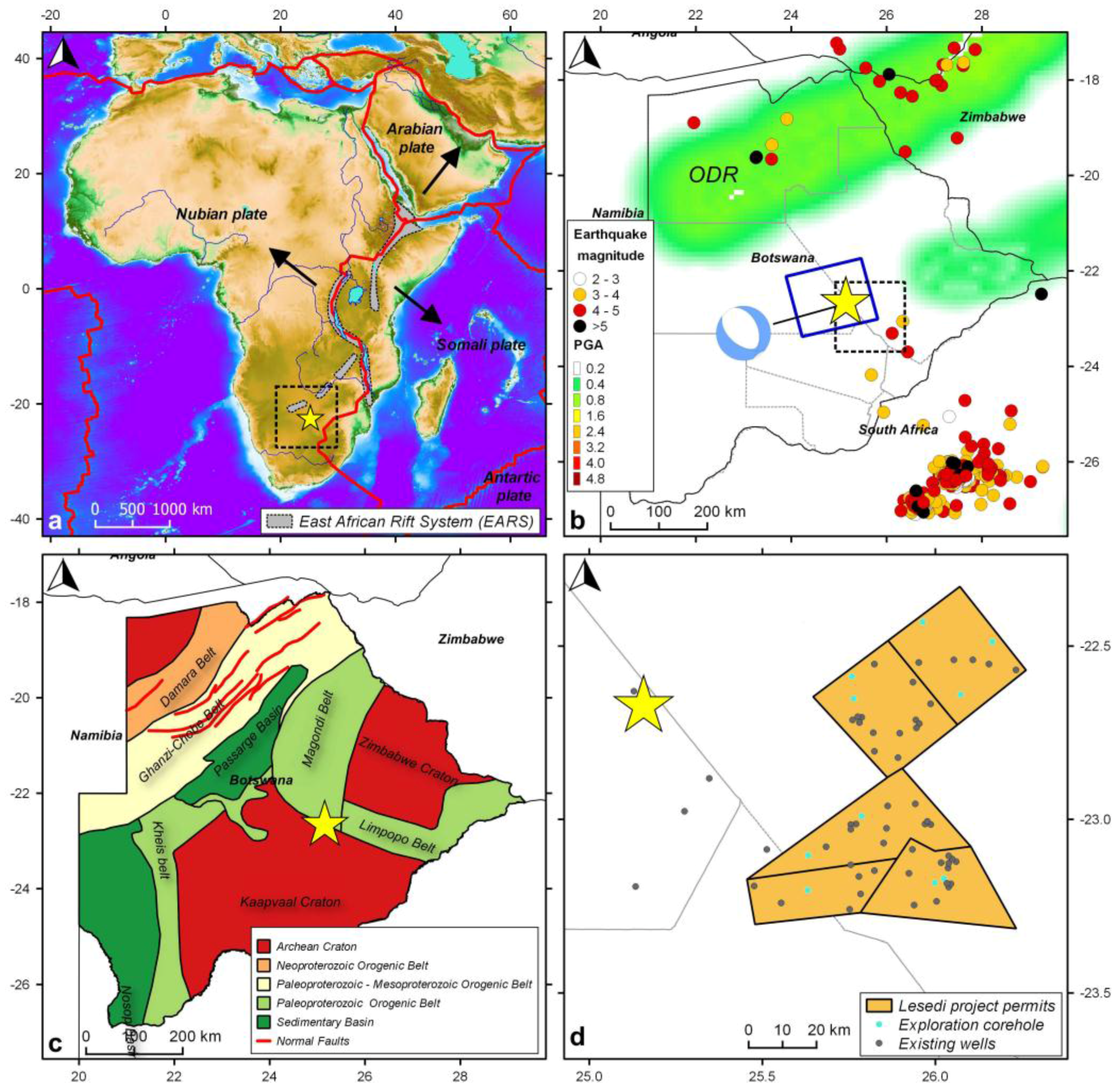
On 3 April 2017, a Mw 6.5 earthquake occurred in the Central District of Botswana, representing the second-strongest earthquake registered since 1949 [1] (Figure 1a). The earthquake was felt by the population of the Botswana capital, Gaborone, and in the neighboring states of South Africa, Zimbabwe and Swaziland, causing 36 injuries [2]. The moment tensor solution of the mainshock (www.globalcmt.org) and the preliminary inversion results of teleseismic body waves (http://geoscope.ipgp.fr/index.php/en/catalog/earthquake-description?seis=us10008e3k) [3] and InSAR data [4] indicate a normal faulting mechanism located at a depth greater than 20 km. (Table S1). The earthquake was followed by few aftershocks to the northeast, with respect to the mainshock, with magnitudes between 4 and 5.
The earthquake occurred over 1000 km from the nearest tectonic plate boundary (Figure 1a), in an area characterized by relatively low seismicity and low seismic hazard [5] (Figure 1b). Indeed, the largest earthquakes in southern Africa are concentrated in the eastern countries of Tanzania, Malawi, and Mozambique, where the continent is slowly pulling apart in an approximately east–west orientation because of the presence of the East African Rift System (EARS) (Figure 1a), thus resulting in normal faults earthquakes.
In Botswana, the past-recorded seismic activity is mainly located in the northwest part of the country, close to the Okavango Delta Region (ODR in Figure 1b), where an incipient arm of the EARS is developing. (Figure 1b,c) [6]. In this area, a major seismic swarm was observed between 1951 and 1953, culminating with the ML 6.1 and 6.7 events on 11 September 1952 and 11 October 1952, respectively [6]. To the south, the epicentral area of the Mw 6.5 event has not experienced strong earthquakes in the past. This area belongs to the Kaapvaal Craton (Figure 1c), composed of Proterozoic and Archean rocks that are 2.5–3.6 billion years old. Cratons are acknowledged as tectonically stable areas and earthquakes occur very rarely.
Given the tectonic assessment of the area, the 3 April 2017 earthquake can be identified as an intraplate earthquake. Although rare, these kind of earthquakes can be rather devastating since they occur far from plate boundaries, in areas scarcely used to deal with such phenomena. For instance, intraplate earthquakes occurred in the US state of Missouri and South Carolina in 1811–1812 and 1886 [7,8]. In 2001, the Indian region of Gujarat was affected by a strong Mw 7.7 intraplate earthquake, causing more than 20,000 casualties [9]. Finally, in 2012, the largest known strike-slip intraplate earthquake (Mw 8.6) occurred in the Indian Ocean, about 100 km SW of the Sumatra subduction zone [10].
With respect to the more common earthquakes occurring at plate boundaries, intraplate earthquakes are poorly understood as most of them are not easily ascribable to any identifiable or prominent fault zone. The causes of these earthquakes are uncertain and often they have been associated with anthropogenic activities such as fluid injection or extraction and hydraulic fracturing [13,14].
The 3 April 2017 Botswana event was even suspected to be an artificial earthquake allegedly triggered by the hydraulic fracking activity [15]. Indeed, in the last decades, the continuous increase of energy demand in southern Africa enhanced the development of projects for the exploitation of natural resources, such as mining and hydrocarbons. These activities have been acknowledged to cause earthquakes, as in the case of the seismic swarm caused by mining in South Africa [3] (Figure 1b). In Botswana, anthropogenic activities consist of the exploitation of Coal-Bed Methane (CBM). In particular, the Lesedi project permits (http://tlouenergy.com/lesedi-cbm-project) managed by the Tolou Energy Limited (TEL) are very close to the 3 April 2017 epicenter area (Figure 1d) and have been active in Botswana since 2014 [16].
Generally, the production of CBM from coal is carried out by decreasing the pore pressure below the coal’s desorption pressure so that methane will desorb from surfaces, diffuse through the coal matrix and become free gas. Typically, coal seams are saturated with water. Thus, the coal must be dewatered for efficient gas production. Dewatering reduces the hydrostatic pressure and promotes gas desorption from coal. In some cases, hydraulic-fracturing is performed for facilitating the dewatering and elevating gas production rates to cost effective levels. Both gas and produced water come to the surface through tubing. Then the gas is sent to a compressor station and into natural gas pipelines, while the produced water is either reinjected into isolated formations, released into streams, used for irrigation, or sent to evaporation ponds.
CBM preliminary operations in the Lesedi project area started in 2009. A great number of exploration wells were drilled in the area to intercept coal-bed methane and to evaluate the commerciality of the gas field (Figure 1d). The performed wells intersected good quality coals at a depth ranging from 300 to 600 m. Afterwards, a pilot program was developed in 2013 in order to simulate a full-scale CBM production. The drilling operations were successfully completed in the middle of 2014, while the dewatering operations and gas productions started at the beginning of the 2014 and continued until 2017 [16].
In this work, we investigate the possible relation between anthropogenic activities and the earthquake occurrence. In particular, we exploit the Synthetic Aperture Radar Interferometry (InSAR) data provided by the Sentinel-1 (S1) mission to explore all the possible seismic source mechanisms associated to the 2017 earthquake. Then, the retrieved fault geometry and mechanism are qualitatively compared with the plausible stress perturbation induced by the anthropogenic activities performed in the area in order to assess the possible interaction between man-made activities and the earthquake occurrence.
2. Materials and Methods
2.1. SAR Data
The InSAR method has become a widely used technique for extracting the deformation of the earth’s surface resulting from natural and anthropic events [17,18,19]. The SAR data used in this study consist in a pair of images acquired along ascending orbit by the Sentinel 1-B (S1B) satellite, the second platform of S1 mission in the framework of the ESA Copernicus program (http://www.copernicus.eu/). They were acquired in the Interferometric Wide Swath (IW) mode on 30 March 2017 and 11 April 2017, i.e., three days before and eight days after the earthquake, respectively. The satellite view geometry, i.e., the incidence angle and the azimuth are equal to 41° and −13°, respectively. We multilooked the images with factors of 24 by 6 along range and azimuth in order to obtain a pixel posting of approximately 90 m, the same resolution of the SRTM DEM used for removing the phase contribution of topography. The perpendicular baseline between the SAR acquisitions is 32 m, thus making negligible the topography-related errors. However, the area covered by the interferogram footprint (approximately 25 km2) (blue rectangle in Figure 1b) presents an almost flat topography, with height variations comprised between 960 and 1140 m above the sea level.
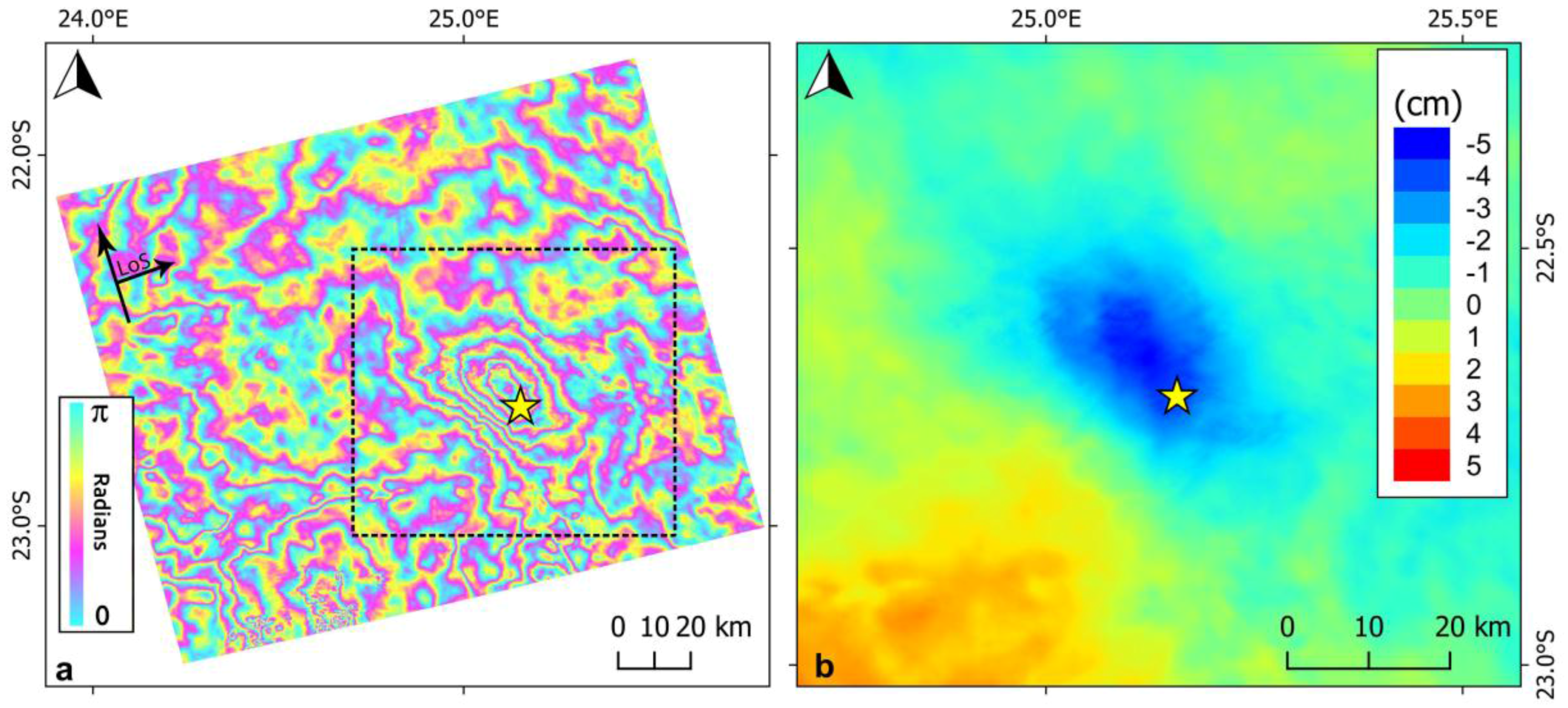
We estimated the differential interferogram using the GAMMA software packages [20]. According to the earthquake epicenter, we selected the S1 subswaths and bursts covering the area of interest (the blue rectangle in Figure 1b). In particular, we used two S1B subswaths and eight bursts for each image for estimating the differential interferogram. The interferogram was filtered with the Goldstein filter [17] to reduce phase noise, and then unwrapped by adopting the minimum cost flow algorithm [21]. The resulting deformation map is shown in Figure 2a. The interferogram was unwrapped and re-wrapped with a color scale ranging from 0 and π, therefore, each color cycle represents a Line of Sight (LoS) deformation of approximately 1.40 cm (i.e., λ/4). The concentric fringe pattern in the interferogram shows that the ground moved away from the satellite, i.e., in the radar LoS, over an area of about 45 by 25 km, extending northwest from the mainshock epicenter. The maximum observed LoS displacement is approximately 5 cm (Figure 2b). The amplitude and extension of the observed ground displacements are compatible with a deep source.
Some atmospheric artifacts are present in the interferogram, which are mainly due to turbulent effects. However, a rough estimation of the LoS tropospheric delay (Figure S1) [22], estimated between the days of the two SAR acquisitions (http://ceg-research.ncl.ac.uk/v2/gacos/), shows that the area surrounding the earthquake epicenter presents a negligible tropospheric delay, which does not affect the observed displacement pattern.
2.2. Data Modelling
As we are primarily interested in finding the fault depth, we inverted the unwrapped interferogram spanning 30 March 2017–11 April 2017 using a nonlinear inversion procedure to constrain the fault geometry with a uniform slip. The Okada [23] formulation for rectangular-plane source in a uniform elastic half-space is adopted to model the observed data.
To perform the inversion, we used the open-source Geodetic Bayesian Inversion Software (GBIS ver. 1.0, Centre for Observation and Modelling of Earthquakes, Volcanoes and Tectonics (COMET), Leeds, England, available at: http://comet.nerc.ac.uk/gbis/) [24] to infer the model parameters by means of the descending interferogram obtained from the S1B satellite data. The inversion code uses a Markov-chain Monte Carlo algorithm, incorporating the Metropolis-Hastings algorithm [25,26,27] to estimate the multivariate posterior probability distribution for all model parameters.
Regarding the InSAR data, the variance-covariance matrix is built assuming that errors in the data can be simulated using an exponential function with nugget, fitted to the isotropic experimental semi-variogram [28]. The experimental semi-variogram and the exponential fit are calculated on the entire InSAR dataset by removing a linear ramp from the data and masking the area showing the surface deformation associated to the earthquake (Figure S2). The parameters of the best-fitting exponential function with nugget, i.e., sill, range and nugget, are 7.5 × 10⁻⁵ m2, 23,190 m and 8.6 × 10⁻¹⁸ m, respectively. Then, the unwrapped interferogram is down-sampled using a quadtree resampling procedure to speed up the calculation process. This resampling technique allows reducing the number of data points with the highest density close to the area affected by the maximum displacement gradient (Figure 3).
The model parameters are location (X-pos. and Y-pos. and Depth in Table 1), size (Length and Width in Table 1) and orientation (Dip and Strike in Table 1) of the fault plane (see Figure S3 for the sign convention). The rake is quantified by the amount of slip estimated along the dip and strike directions (Strike slip and Dip slip in Table 1). The Harvard CMT solution is used as initial parameters in the inversion procedure. All the fault parameters are allowed to vary between the intervals reported in Table 1. In particular, both normal and thrust mechanisms are investigated by allowing the dip and the slip along the strike and dip directions to vary between ±90° and ±5 m, respectively.
3. Results
In Figure 4, we show the comparison between observed displacements, model prediction, and residuals. Optimal model parameters are reported in Table 1, and full a-posteriori probability density functions and trade-offs between fault parameters are shown in Figure 5. Assuming a rigidity modulus of 30 GPa, the computed optimal solution presents a seismic moment equal to 6.14 × 10¹⁸ Nm, corresponding to a moment magnitude of 6.46, in agreement with the CMT solution (www.globalcmt.org).
The retrieved optimal parameters define a northwest striking, northeast dipping normal fault (center panels in Figure 4), which reproduces the field observations remarkably well. Indeed, the residuals in the simulated LoS displacements are lower than 1 cm in the area affected by the maximum displacement. The retrieved fault position, geometry and mechanism fairly agree with the CMT solution and with a previous forward modelling of InSAR data performed by Kolawole et al. [4] (Table S1). On the contrary, the estimated resultant slip and rake (approximately 2.7 m and −131°) slightly differ from previous inversion of InSAR data [4], thus identifying a predominant right-lateral dislocation component. It is noteworthy that Kolawole et al. [4] performed the inversion of InSAR data by fixing the fault rake while we allowed the rake to vary between 0–360°, according to the selected bounds for the strike and dip slip components (Table 1).
The a-posteriori probability distribution function of fault parameters (Figure 5 and Table 2) show a discrete variability of the retrieved fault parameters, especially for the length and width of the fault plane and for the amount of slip along the rake direction, whose trade-off is well known [29] (Figure 5), especially when only one InSAR LoS measurement is used. The other parameters are estimated fairly well. In particular, the source depth is certainly greater than 20 km, thus confirming the deep source of the event, and the dip slip component variability is comprised between negative values (Table 2), thus confirming a normal faulting mechanism (Figure S3).
4. Discussion
The results of the inversion procedure are in agreement with the tectonic and geodynamic assessment of the area. Indeed, the earthquake epicenter is located in an extensional area (Figure 6a), where a new rifting zone is developing [30]. Moreover, the retrieved fault geometry (i.e., strike and dip) is consistent with the tectonic structures inferred from 3D aeromagnetic and gravimetric data [4] (Figure 6b).
Given the fault geometry and the tectonic assessment of the area, we investigate the relationship between anthropogenic activities and the initiation of the Mw 6.5 earthquake. The potential for anthropogenic activities to trigger earthquakes has been widely acknowledged by the scientific community [31,32,33,34]. In particular, the generation mechanisms and magnitudes of anthropogenic earthquakes depend on several factors, such as the volume of the injected or extracted fluids, the extent of the perturbation [35], the geometry and orientation of the fault planes, the hydraulic connection between the injection and extraction zones and the fault planes [14], the magnitude of the tectonic stress field, and the distance between anthropogenic activities and earthquake source.
The possible triggering of the 3 April 2017 earthquake by anthropogenic activities has been investigated by analyzing the compatibility between the potential stress perturbation at depth induced by anthropogenic activities and the retrieved earthquake geometry and fault mechanism.
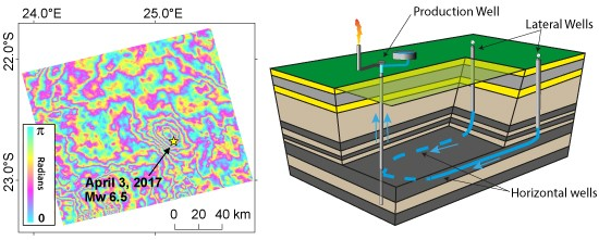
Actually, the drilling program at the Lesedi project area comprises two pilot pods, called Selemo and Lesedi (Figure 6b). Each pod is composed by a vertical well and two horizontal wells, which start from the vertical one and develop for 750 m into the coal seam (Figure 7). The horizontal wells intercept the lower Morupule Coal Seam at a depth of approximately 450 m (Figure 7). Thus, the distance at depth between production wells and the retrieved earthquake source is greater than 20 km.
Such a great distance could not exclude any possible interaction because, depending on the type of the performed anthropogenic activity, many strong earthquakes have been triggered at up to 30 km distance [32,36,37]. It is then necessary to analyze the type of anthropogenic activity performed at the Lesedi CBM project area in order to define the hypothetical stress pattern produced at depth.
The production of CBM from the Selemo and Lesedi pilot pods is performed by dewatering the coal by means of submerged pumps. Actually, there is no stimulation with the hydraulic-fracturing technique. The extracted water is disposed through evaporation ponds, thus, no injection activities are conducted in the area [16] (Figure 7). Hence, the major source of stress at depth is the dewatering of the coal and the compaction of the reservoir because of CBM extraction.
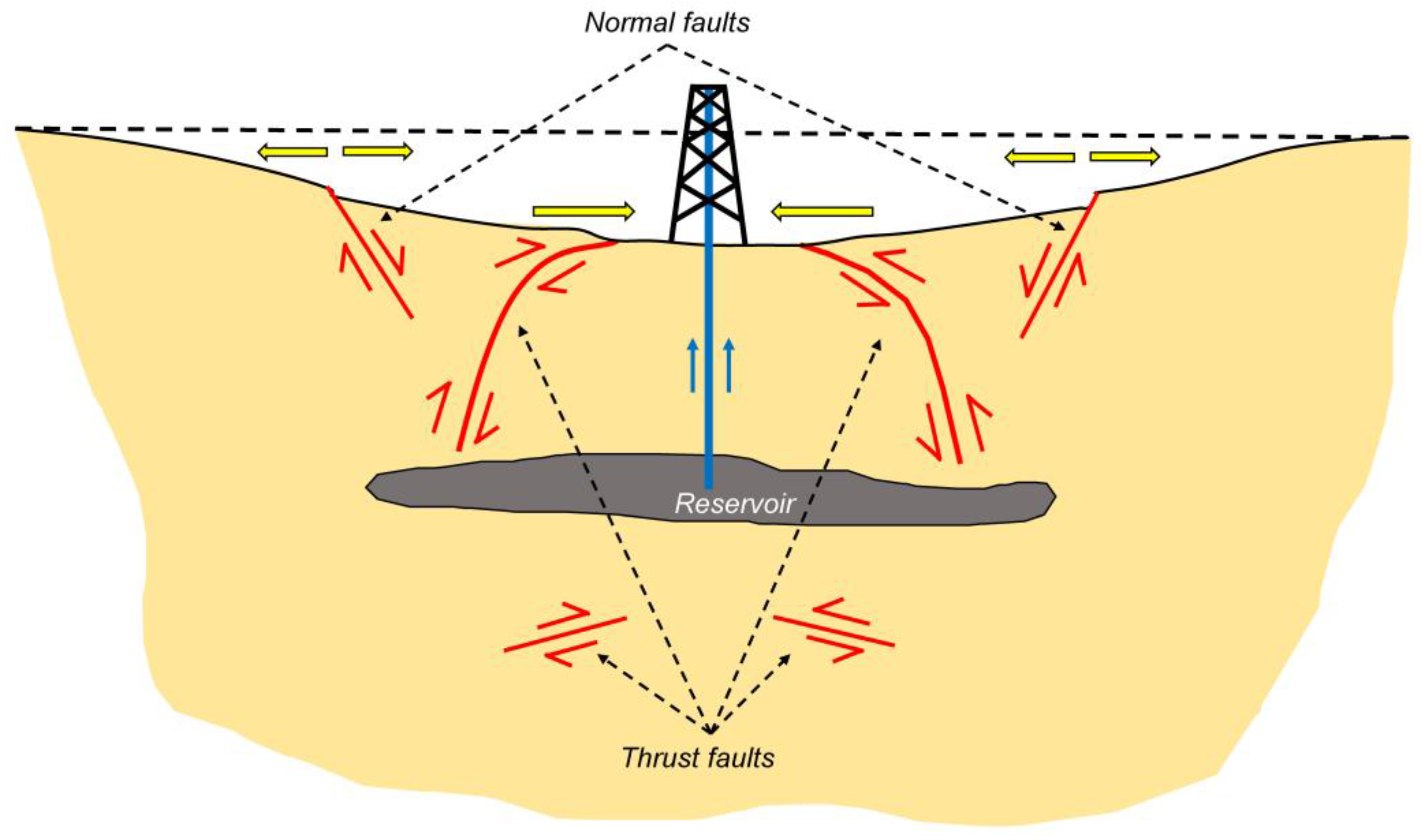
When a fluid is extracted, pore pressures decline causing the permeable reservoir rocks to contract, thus modifying the stresses in the neighboring crust. In particular, the CBM operations performed at the Lesedi project area can be schematized as a fluid withdrawal from a permeable layer embedded in a fluid-infiltrated, impermeable half-space. Analytical and analogical simulations based on such a simplified scheme show that the induced mean stress is compressive below and above the point of extraction and slightly extensional along the flanks of the reservoir. Over time, the extensional zones migrate further outward and compressive zones further down. Consequently, reverse faulting is favored above and below the reservoir, while normal faulting is favored along the flanks of the reservoir [38,39,40,41] (Figure 8). The normal fault associated to the Mw 6.5 Botswana earthquake is located more than 20 km below the CBM reservoir, where the potential anthropogenic stress changes are compressive and thrust faulting is privileged with respect to normal faulting. Consequently, the potential stress field caused by the CBM operations is not compatible with the Botswana earthquake, which is likely to be a natural intraplate earthquake caused by rifting [4].
5. Conclusions
We qualitatively investigated the connection between anthropogenic activities and the occurrence of the 3 April 2017, Mw 6.5 Botswana earthquake. The coseismic displacement field retrieved from S1B SAR data produced very important information for the first assessment of the earthquake scenario and allowed the fast identification of the finite seismic source. Thanks to the qualitative assessment of the hypothetical stress perturbations induced by CBM extractions, we can exclude any possible interaction between anthropogenic activities and the earthquake occurrence. However, the available data did not allow to quantitatively estimate the anthropogenic stress perturbation at depth. More detailed and quantitative investigation are needed in the future in order to assess the impact of stress perturbations induced by anthropogenic activities in Botswana.
Supplementary Materials
The following are available online at www.mdpi.com/2072-4292/9/10/1028/s1, Figure S1: (a) Detail of the area bordered by the dashed black square in Figure 2a, showing the unwrapped interferogram; (b) Estimated Zenith Path Delay Difference Map (http://ceg-research.ncl.ac.uk/v2/gacos/) [22], projected along the satellite LoS. The area and the colormap are the same of panel (a); Figure S2: Estimation of the experimental semi-variogram on the de-trended dataset and fit with an exponential function with nugget. (a) Original wrapped dataset (the earthquake area is masked); (b) estimated linear ramp removed from the data; (c) de-trended wrapped dataset; (d) experimental semi-variogam calculated on the original dataset; (e) experimental semi-variaogam (red squares) calculated on the de-trended dataset and exponential fit with nugget (blue line); Figure S3: Sign convention adopted in the inversion procedure (modified from http://comet.nerc.ac.uk/gbis/); Table S1: Fault parameters from the CMT solution and the inversion of teleseismic body waves (http://geoscope.ipgp.fr/index.php/en/catalog/earthquake-description?seis=us10008e3k) [3] and InSAR data [4].
Acknowledgments
The authors thank the European Space Agency for providing the Sentinel-1 SAR data.
Author Contributions
Matteo Albano and Marco Polcari developed the project, analyzed and interpreted the data and wrote the paper. Marco Polcari, Christian Bignami and Salvatore Stramondo processed the SAR data. Marco Moro and Michele Saroli gave the geological and tectonic conceptual model of the area. Matteo Albano and Michele Saroli performed the conceptual and analytical modeling and the comparison with anthropogenic activities. All authors read and approved the final manuscript.
Conflicts of Interest
The authors declare no conflict of interest.
References
- Simon, R.; Kwadiba, M.; King, J.; Moidaki, M. A history of Botswana’s seismic network. Botsw. Notes Rec. 2012, 44, 184–192. [Google Scholar] [CrossRef]
- Koothupile, B. Botswana Quake: At Least 36 Students “Affected”, Structural “Defects” Reported. Available online: http://www.news24.com/Africa/News/botswana-quake-at-least-36-students-injured-structural-defects-reported-20170404 (accessed on 3 May 2017).
- Vallée, M.; Charléty, J.; Ferreira, A.M.G.; Delouis, B.; Vergoz, J. SCARDEC: A new technique for the rapid determination of seismic moment magnitude, focal mechanism and source time functions for large earthquakes using body-wave deconvolution. Geophys. J. Int. 2011, 184, 338–358. [Google Scholar] [CrossRef]
- Kolawole, F.; Atekwana, E.A.; Malloy, S.; Stamps, D.S.; Grandin, R.; Abdelsalam, M.G.; Leseane, K.; Shemang, E.M. Aeromagnetic, gravity, and Differential Interferometric Synthetic Aperture Radar (DInSAR) analyses reveal the causative fault of the 3 April 2017 Mw 6.5 Moiyabana, Botswana Earthquake. Geophys. Res. Lett. 2017, 44, 8837–8846. [Google Scholar] [CrossRef]
- Giardini, D.; Grünthal, G.; Shedlock, K.M.; Zhang, P. The GSHAP Global Seismic Hazard Map. In International Handbook of Earthquake & Engineering Seismology; Lee, W., Kanamori, H., Jennings, P., Kisslinger, C., Eds.; Academic Press: Amsterdam, The Netherlands, 2003; pp. 1233–1239. [Google Scholar]
- Reeves, C.V. Rifting in the Kalahari? Nature 1972, 237, 95–96. [Google Scholar] [CrossRef]
- Tuttle, M.P. The earthquake potential of the New Madrid seismic zone. Bull. Seismol. Soc. Am. 2002, 92, 2080–2089. [Google Scholar] [CrossRef]
- Bakun, W.H.; Hopper, M.G. Magnitudes and locations of the 1811–1812 New Madrid, Missouri, and the 1886 Charleston, South Carolina, earthquakes. Bull. Seismol. Soc. Am. 2004, 94, 64–75. [Google Scholar] [CrossRef]
- Saito, K.; Spence, R.J.S.; Going, C.; Markus, M. Using high-resolution satellite images for post-earthquake building damage assessment: A study following the 26 January 2001 Gujarat earthquake. Earthq. Spectra 2004, 20, 145–169. [Google Scholar] [CrossRef]
- Yadav, R.K.; Kundu, B.; Gahalaut, K.; Catherine, J.; Gahalaut, V.K.; Ambikapthy, A.; Naidu, M.S. Coseismic offsets due to the 11 April 2012 Indian Ocean earthquakes (Mw 8.6 and 8.2) derived from GPS measurements. Geophys. Res. Lett. 2013, 40, 3389–3393. [Google Scholar] [CrossRef]
- Bird, P. An updated digital model of plate boundaries. Geochem. Geophys. Geosyst. 2003, 4. [Google Scholar] [CrossRef]
- Leseane, K.; Atekwana, E.A.; Mickus, K.L.; Abdelsalam, M.G.; Shemang, E.M.; Atekwana, E.A. Thermal perturbations beneath the incipient Okavango Rift Zone, northwest Botswana. J. Geophys. Res. Solid Earth 2015, 120, 1210–1228. [Google Scholar] [CrossRef]
- Keranen, K.M.; Savage, H.M.; Abers, G.A.; Cochran, E.S.; Humphreys, E.; Karlstrom, K.; Ekström, G.; Carlson, C.; Dixon, T.; Gurnis, M.; et al. Potentially induced earthquakes in Oklahoma, USA: Links between wastewater injection and the 2011 Mw 5.7 earthquake sequence. Geology 2013, 41, 699–702. [Google Scholar] [CrossRef]
- Ellsworth, W.L. Injection-induced earthquakes. Science 2013, 341, 142–149. [Google Scholar] [CrossRef] [PubMed]
- Barbee, J. Did Fracking in Botswana Cause Johannesburg to Tremble? Available online: https://www.dailymaverick.co.za/article/2017-04-04-did-fracking-in-botswana-cause-johannesburg-to-tremble/#.WSWA-2jyi72 (accessed on 5 May 2017).
- Tlou Energy Ltd. Tlou Energy Limited Annual Report (2010–2016). Available online: http://tlouenergy.com/reports (accessed on 5 July 2017).
- Stramondo, S.; Trasatti, E.; Albano, M.; Moro, M.; Chini, M.; Bignami, C.; Polcari, M.; Saroli, M. Uncovering deformation processes from surface displacements. J. Geodyn. 2016, 102, 58–82. [Google Scholar] [CrossRef]
- Sharma, R.C.; Tateishi, R.; Hara, K.; Nguyen, H.T.; Gharechelou, S.; Nguyen, L.V. Earthquake Damage Visualization (EDV) technique for the rapid detection of earthquake-induced damages using SAR data. Sensors 2017, 17, 235. [Google Scholar] [CrossRef] [PubMed]
- Hu, J.; Wang, Q.; Li, Z.; Zhao, R.; Sun, Q. Investigating the ground deformation and source model of the Yangbajing geothermal field in Tibet, China with the WLS InSAR technique. Remote Sens. 2016, 8, 191. [Google Scholar] [CrossRef]
- Wegmuller, U.; Werner, C. Gamma SAR processor and interferometry software. In ERS Symposium on Space at the Service of Our Environment; ESA Publications Division: Florence, Italy, 1997; pp. 1687–1692. [Google Scholar]
- Costantini, M. A novel phase unwrapping method based on network programming. IEEE Trans. Geosci. Remote Sens. 1998, 36, 813–821. [Google Scholar] [CrossRef]
- Yu, C.; Penna, N.T.; Li, Z. Generation of real-time mode high-resolution water vapor fields from GPS observations. J. Geophys. Res. Atmos. 2017, 122, 2008–2025. [Google Scholar] [CrossRef]
- Okada, Y. Surface deformation due to shear and tensile faults in a half-space. Bull. Seismol. Soc. Am. 1985, 75, 1135–1154. [Google Scholar]
- Bagnardi, M.; Hooper, A. Bayesian inversion of surface deformation data for rapid estimate of source parameters: A proposed approach. 2017; (in prep.). [Google Scholar]
- Hastings, W.K. Monte Carlo sampling methods using Markov chains and their applications. Biometrika 1970, 57, 97–109. [Google Scholar] [CrossRef]
- Mosegaard, K.; Tarantola, A. Monte Carlo sampling of solutions to inverse problems. J. Geophys. Res. Solid Earth 1995, 100, 12431–12447. [Google Scholar] [CrossRef]
- Hopper, A.; Pietrzak, J.; Simons, W.; Cui, H.; Riva, R.; Naeije, M.; Terwisscha van Scheltinga, A.; Schrama, E.; Stelling, G.; Socquet, A. Importance of horizontal seafloor motion on tsunami height for the 2011 Mw = 9.0 Tohoku-Oki earthquake. Earth Planet. Sci. Lett. 2013, 361, 469–479. [Google Scholar] [CrossRef]
- Webster, R.; Oliver, M.A. Geostatistics for Environmental Scientists, 2nd ed.; John Wiley & Sons Inc.: Chichester, UK, 2007; ISBN 978-0-470-02858-2. [Google Scholar]
- Atzori, S.; Antonioli, A. Optimal fault resolution in geodetic inversion of coseismic data. Geophys. J. Int. 2011, 185, 529–538. [Google Scholar] [CrossRef] [Green Version]
- Chisenga, C. Understanding the Earth Structure Underneath Botswana: The Tectonic Model and Its Relationship to the Basement and Crustal Thickness. Master’s Thesis, University of Twente, Enschede, The Netherlands, 2015. [Google Scholar]
- Albano, M.; Barba, S.; Tarabusi, G.; Saroli, M.; Stramondo, S. Discriminating between natural and anthropogenic earthquakes: Insights from the Emilia Romagna (Italy) 2012 seismic sequence. Sci. Rep. 2017, 7, 282. [Google Scholar] [CrossRef] [PubMed]
- Davies, R.; Foulger, G.; Bindley, A.; Styles, P. Induced seismicity and hydraulic fracturing for the recovery of hydrocarbons. Mar. Pet. Geol. 2013, 45, 171–185. [Google Scholar] [CrossRef] [Green Version]
- McGarr, A.; Simpson, D.; Seeber, L. Case histories of induced and triggered seismicity. Int. Geophys. 2002, 81, 647–661. [Google Scholar] [CrossRef]
- Suckale, J. Moderate-to-large seismicity induced by hydrocarbon production. Lead. Edge 2010, 29, 310–319. [Google Scholar] [CrossRef]
- McGarr, A.; Bekins, B.; Burkardt, N.; Dewey, J.; Earle, P.; Ellsworth, W.; Ge, S.; Hickman, S.; Holland, A.; Majer, E.; et al. Coping with earthquakes induced by fluid injection. Science 2015, 347, 830–831. [Google Scholar] [CrossRef] [PubMed]
- Mulargia, F.; Bizzarri, A. Anthropogenic Triggering of Large Earthquakes. Sci. Rep. 2015, 4, 6100. [Google Scholar] [CrossRef] [PubMed]
- Liu, S.; Xu, L.; Talwani, P. Reservoir-induced seismicity in the Danjiangkou Reservoir: A quantitative analysis. Geophys. J. Int. 2011, 185, 514–528. [Google Scholar] [CrossRef]
- Segall, P. Earthquakes triggered by fluid extraction. Geology 1989, 17, 942–946. [Google Scholar] [CrossRef]
- Baranova, V.; Mustaqeem, A.; Bell, S. A model for induced seismicity caused by hydrocarbon production in the Western Canada sedimentary basin. Can. J. Earth Sci. 1999, 36, 47–64. [Google Scholar] [CrossRef]
- Segall, P. Stress and subsidence resulting from subsurface fluid withdrawal in the epicentral region of the 1983 Coalinga Earthquake. J. Geophys. Res. 1985, 90, 6801–6816. [Google Scholar] [CrossRef]
- Odonne, F.; Ménard, I.; Massonnat, G.J.; Rolando, J.P. Abnormal reverse faulting above a depleting reservoir. Geology 1999, 27, 111–114. [Google Scholar] [CrossRef]
Figure 1.
(a) Location of the 3 April 2017 , Mw 6.5 Botswana earthquake (the yellow star) with respect to the plate boundaries (red lines) and the East African Rift System [11]. (b) Detail of the area bordered by the dashed black square in panel (a), showing the location of historical earthquakes (https://earthquake.usgs.gov/earthquakes/map/) and the seismic hazard map [5] of Botswana. The earthquakes span from 1950 to 2016. The seismic hazard map shows the Peak Ground Acceleration (PGA) (m·s2) with a 10% exceedance probability in 50 years. The earthquakes in South Africa are caused by mining activities (http://inducedearthquakes.org/). (c) Precambrian tectonic map of Botswana outlining the spatial extent of Archean cratons and Proterozoic orogenic belts. Red lines represent the fault system of the Okavango Delta rift zone (modified form Leseane et al. [12]). (d) Detail of the area bordered by the dashed black square in panel (b), showing the location of the Lesedi project permits (http://tlouenergy.com/lesedi-cbm-project) respect to the 3 April 2017 earthquake. Coordinates are in the wgs84 datum.

Figure 2.
(a) Wrapped interferogram showing the co-seismic displacement induced by the Mw 6.5, 2017 Botswana earthquake. The interferogram’s footprint corresponds to the blue rectangle in Figure 1b). The interferogram was re-wrapped with a color scale ranging from 0 and π then each color cycle represents a LoS deformation of approximately 1.40 cm (i.e., λ/4). (b) Detail of the area bordered by the dashed black square in panel (a), showing the unwrapped interferogram. The yellow star indicates the earthquake epicenter (https://earthquake.usgs.gov/earthquakes/eventpage/us10008e3k#executive). Coordinates are in the wgs84 datum.

Figure 3.
Down-sampled interferogram data of the area bordered by the dashed black square in Figure 2a using the quadtree decomposition algorithm. Negative values indicate motion away from the satellite along its LoS, while positive values indicate motion toward the satellite. Coordinates refer to a local origin (Longitude = 25.12°; Latitude = −22.63°).
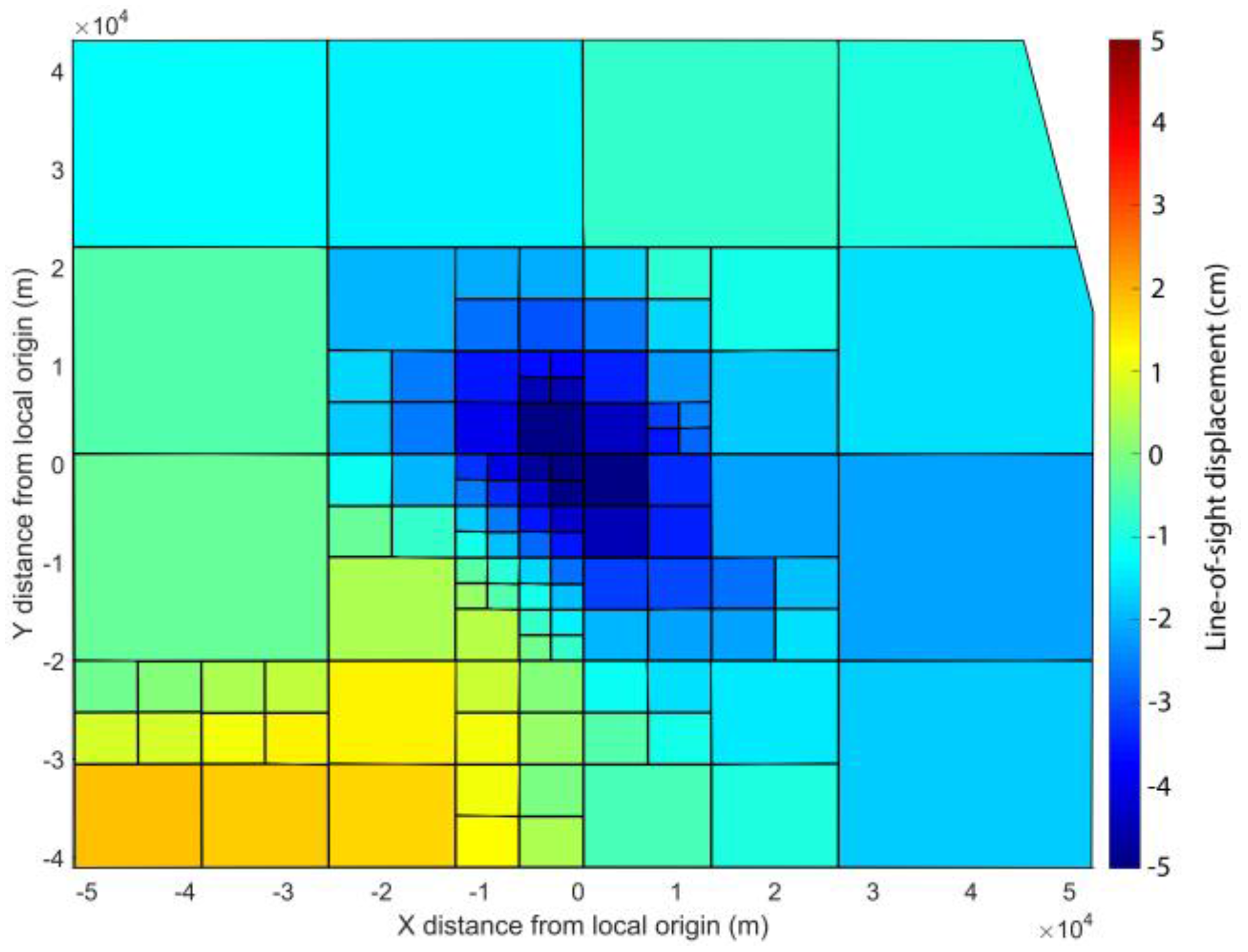
Figure 4.
InSAR data and elastic dislocation model for the 3 April 2017 earthquake. Left panels: stack of the wrapped and unwrapped ascending track S1B SAR interferogram spanning the interval 30 March–11 April. Center panels: wrapped and unwrapped best-fitting elastic dislocation model for uniform slip on a rectangular plane obtained from the inversion of InSAR data. The solid black line shows the surface trace of the uniform slip solution, while the dashed black rectangle shows the location of the fault plane at depth. The yellow star locates the epicenter of the mainshock. Right panels: wrapped and unwrapped residuals between the data and the model. Coordinates refer to a local origin (Longitude = 25.12° and Latitude = −22.63°).
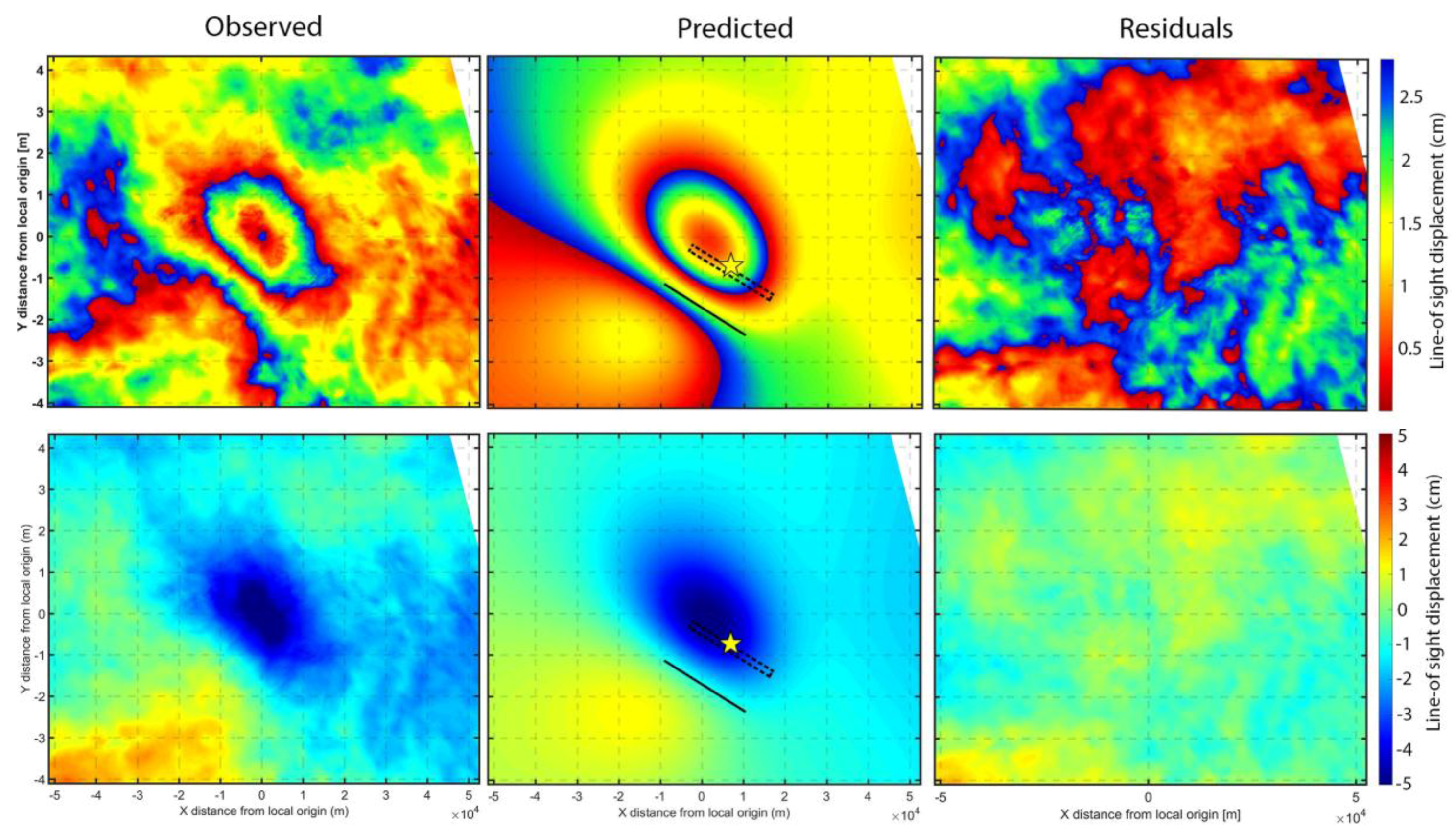
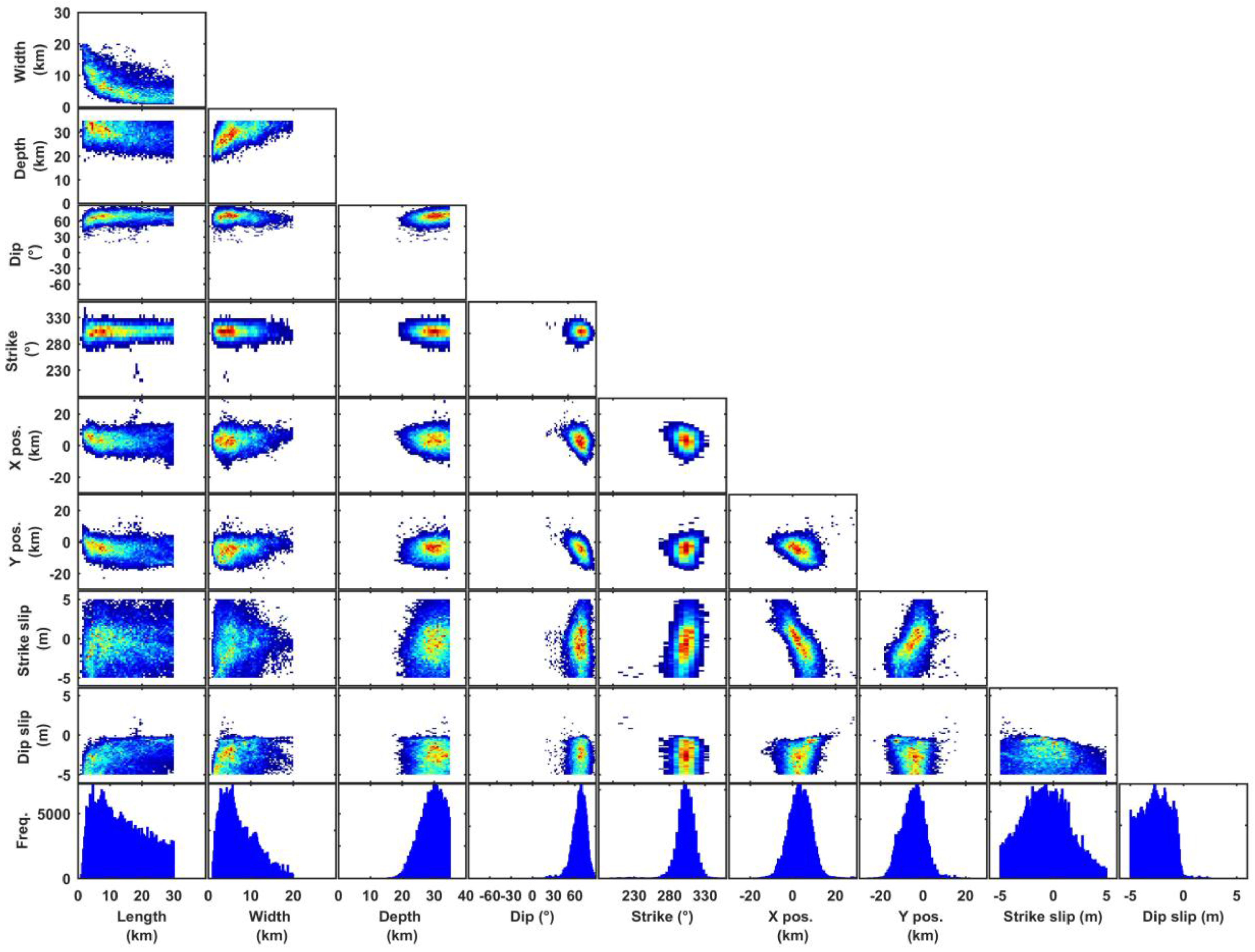
Figure 5.
Fault parameter uncertainties and trade-offs for the uniform slip InSAR model of the 3 April 2017 Mw 6.5 earthquake. Uncertainties and trade-offs are calculated using a Monte Carlo approach from the inversion of 1 × 10⁶ datasets perturbed with realistic noise. Histograms show the a-posteriori probability distribution of fault parameters, and scatterplots show trade-offs between parameters. The a-priori bounds are listed in Table 1.

Figure 6.
(a) Location of the 3 April 2017 Mw 6.5 Botswana earthquake on the map showing the crustal thickness of Botswana (contours) and the geodynamic interpretation. Figure modified from Chisenga [30]. The gray lines indicate the major tectonic province and the letters represent names of tectonic province: NWS = north western group, ZC = Zimbabwe craton, RC = Roibok complex, KC = kwando complex, GCZ = Ghanzi-Chobe zone, NBR = North Botswana rift, PB = passarge basin, XC = Xadi complex, MB = Magondi belt, LB = Limpopo belt, OB = Okwa belt, TC = Tshane belt, KB = Kheis belt, NB = Nossop basin and KB = Kaapvaal belt. (b) Detail of the area bordered by the dashed black square in panel (a), showing the location of the retrieved fault geometry respect to the Lesedi project permits (http://tlouenergy.com/lesedi-cbm-project) and the tectonic structures inferred from 3D aeromagnetic and gravity data [4]. The colored map shows the LoS ground displacements from InSAR data (see Figure 2b). Coordinates are in the wgs84 datum.
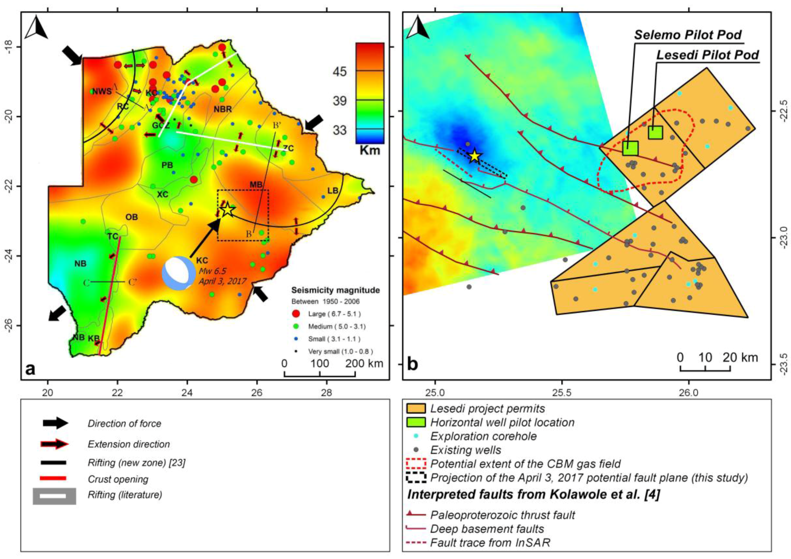
Figure 7.
Simplified 3D sketch (modified from http://tlouenergy.com/lesedi-cbm-project) of the Selemo and Lesedi pilot Pod areas of Figure 1d. The CBM is extracted from the two horizontal wells, which are connected to a vertical production well. The two lateral wells are closed.
Figure 7.
Simplified 3D sketch (modified from http://tlouenergy.com/lesedi-cbm-project) of the Selemo and Lesedi pilot Pod areas of Figure 1d. The CBM is extracted from the two horizontal wells, which are connected to a vertical production well. The two lateral wells are closed.
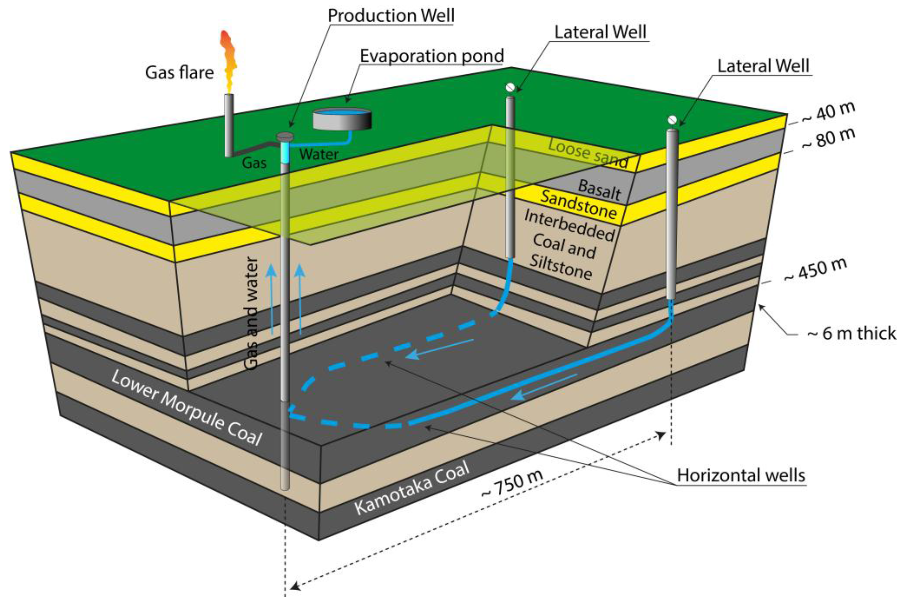
Figure 8.
Schematic cross section (modified from Odonne et al., [41]) summarizing the surface deformation and faulting (red lines) associated with fluid withdrawal. Normal faults develop on flanks of field while reverse faults develop over and below reservoir, and close to Earth’s surface. The yellow arrows indicate horizontal displacement at Earth’s surface.

Table 1.
Fault parameter intervals and best fit solution resulting from the nonlinear inversion.
| Parameter | Length (km) | Width (km) | Depth (km) | Dip (°) | Strike (°) | X-pos. 1 (km) | Y-pos. 1 (km) | Strike slip (m) | Dip slip (m) |
|---|---|---|---|---|---|---|---|---|---|
| Start | 26 | 12 | 20 | 53 | 320 | 0 | 0 | 0.5 | 0.5 |
| Lower bound | 1 | 1 | 0.1 | −90 | 180 | −30 | −30 | −5 | −5 |
| Upper bound | 30 | 20 | 35 | 90 | 360 | 30 | 30 | 5 | 5 |
| Optimal | 21 | 3.6 | 25 | 65 | 304 | 6.4 | −8.1 | −1.97 | −1.85 |
1 Starting values of X- and Y- position correspond to Longitude = 25.12° and Latitude = −22.63°. Coordinates are referred to the mid-point of the fault horizontal edge (Figure S3).
Table 2.
Optimal fault parameters and range of variability.
| Parameter | Optimal | Mean | Median | 95% Confidence Interval | ||
|---|---|---|---|---|---|---|
| Length (km) | 21.1 | 13.6 | 12.5 | 2.3 | - | 28.9 |
| Width (km) | 3.6 | 7.2 | 6.2 | 1.6 | - | 17.1 |
| Depth (km) | 25.2 | 29.1 | 29.5 | 21.4 | - | 34.6 |
| Dip (°) | 65.5 | 66.4 | 67.4 | 44.6 | - | 82.2 |
| Strike (°) | 304.4 | 302.4 | 303 | 277.5 | - | 324.5 |
| X-pos. (km) | 6.4 | 3.3 | 3.4 | −7 | - | 12.9 |
| Y-pos. (km) | −8.1 | −4.7 | −4.6 | −14.7 | - | 5.5 |
| Strike slip (m) | −1.97 | −0.65 | −0.71 | −4.6 | - | 3.9 |
| Dip slip (m) | −1.85 | −2.62 | −2.6 | −4.87 | - | −0.45 |
© 2017 by the authors. Licensee MDPI, Basel, Switzerland. This article is an open access article distributed under the terms and conditions of the Creative Commons Attribution (CC BY) license (http://creativecommons.org/licenses/by/4.0/).
Share and Cite
MDPI and ACS Style
Albano, M.; Polcari, M.; Bignami, C.; Moro, M.; Saroli, M.; Stramondo, S. Did Anthropogenic Activities Trigger the 3 April 2017 Mw 6.5 Botswana Earthquake? Remote Sens. 2017, 9, 1028. https://doi.org/10.3390/rs9101028
AMA Style
Albano M, Polcari M, Bignami C, Moro M, Saroli M, Stramondo S. Did Anthropogenic Activities Trigger the 3 April 2017 Mw 6.5 Botswana Earthquake? Remote Sensing. 2017; 9(10):1028. https://doi.org/10.3390/rs9101028
Chicago/Turabian StyleAlbano, Matteo, Marco Polcari, Christian Bignami, Marco Moro, Michele Saroli, and Salvatore Stramondo. 2017. "Did Anthropogenic Activities Trigger the 3 April 2017 Mw 6.5 Botswana Earthquake?" Remote Sensing 9, no. 10: 1028. https://doi.org/10.3390/rs9101028
Note that from the first issue of 2016, this journal uses article numbers instead of page numbers. See further details here.