Assessing and Improving the Reliability of Volunteered Land Cover Reference Data
by
 , , and
Yuanyuan Zhao
1, 
Duole Feng
1,
Le Yu
1,
Linda See
2 ,
,
Steffen Fritz
2,
Christoph Perger
2 and
Peng Gong
1,* 1
Ministry of Education Key Laboratory for Earth System Modeling, Department of Earth System Science, Tsinghua University, Beijing 100084, China
2
International Institute for Applied Systems Analysis, Laxenburg A-2361, Austria
*
Author to whom correspondence should be addressed.
Remote Sens. 2017, 9(10), 1034; https://doi.org/10.3390/rs9101034
Submission received: 22 August 2017
/
Revised: 1 October 2017
/
Accepted: 4 October 2017
/
Published: 10 October 2017
Abstract
:Volunteered geographic data are being used increasingly to support land cover mapping and validation, yet the reliability of the volunteered data still requires further research. This study proposes data-based guidelines to help design the data collection by assessing the reliability of volunteered data collected using the Geo-Wiki tool. We summarized the interpretation difficulties of the volunteers at a global scale, including those areas and land cover types that generate the most confusion. We also examined the factors affecting the reliability of majority opinion and individual classification. The results showed that the highest interpretation inconsistency of the volunteers occurred in the ecoregions of tropical and boreal forests (areas with relatively poor coverage of very high resolution images), the tundra (a unique region that the volunteers are unacquainted with), and savannas (transitional zones). The volunteers are good at identifying forests, snow/ice and croplands, but not grasslands and wetlands. The most confusing pairs of land cover types are also captured in this study and they vary greatly with different biomes. The reliability can be improved by providing more high resolution ancillary data, more interpretation keys in tutorials, and tools that assist in coverage estimation for those areas and land cover types that are most prone to confusion. We found that the reliability of the majority opinion was positively correlated with the percentage of volunteers selecting this choice and negatively related to their self-evaluated uncertainty when very high resolution images were available. Factors influencing the reliability of individual classifications were also compared and the results indicated that the interpretation difficulty of the target sample played a more important role than the knowledge base of the volunteers. The professional background and local knowledge had an influence on the interpretation performance, especially in identifying vegetation land cover types other than croplands. These findings can help in building a better filtering system to improve the reliability of volunteered data used in land cover validation and other applications.
1. Introduction
Land cover and land cover change data are an essential input to a wide range of applications, e.g., Earth system modeling, urban planning, resource management, and biodiversity conservation, among others [1,2,3]. Therefore, accurate and up-to-date land cover maps are required. It is widely accepted that training and reference samples are very important in producing and validating land cover maps. The collection of large samples of high quality reference data, whether through field surveys or expert interpretation of imagery, is very expensive, and thus alternative data collection approaches are often desired.
In recent years, volunteered geographic information (VGI) [4] has emerged as a new source of data that has been shown to support different applications, e.g., disaster management [5,6,7], urban and transportation planning [8], and land use management [9]. With potentially large volumes of data at relatively low costs, VGI has also been identified as a good source of data for Earth observation, in particular for land cover validation [10,11,12,13]. In addition to validation, VGI can also be used as a potential source of training data for land cover classification algorithms [14,15] and land cover change detection [16], as well as building hybrid land cover products [17,18].
However, there are many concerns about the reliability of volunteered land cover reference data [19]. A few studies have evaluated the quality of volunteer contributions to land cover mapping [20,21] where the results from these studies emphasized the importance of control or expert data in evaluating the performance of the volunteer. They also provided some methods to measure the reliability of the volunteered land cover information. However, it is time-consuming to build a global control data set. Consensus-based data quality assessment is an alternative that is relatively easy to implement [22].
Another aspect of studies in VGI is the exploration of the effect of performance based on factors related to contributors such as their backgrounds. For example, little difference was found between experts and non-experts in the domain of remote sensing in identifying human impact from very high resolution imagery, yet the experts were slightly better than non-experts in classifying land cover [23]. The impact of local knowledge on aiding classification performance was found to have little effect in identifying cropland from very high resolution imagery in the Cropland Capture game [24]. The study also found that the volunteers with a professional background in remote sensing did no better than common volunteers at this task. However, since croplands are easier to differentiate and have less spatial variation than other vegetation types, there are still open questions related to the impact of local knowledge on the identification of other land cover types. There are other concerns that factors like differences in landscape conceptualization will have impacts on the crowdsourced data. Another study has shown that there are differences in the crowdsourced land cover data contributed by different groups, based on nationality and on domain experience [25]. However, the influence of other factors such as how much volunteers know about a given place for which they are making an interpretation (e.g., the local climate type) still remains unclear. Among all the different factors that could influence performance including the interpretation difficulty of the target sample and the knowledge base of the volunteers, which play the most important role? These are still outstanding questions that need to be answered.
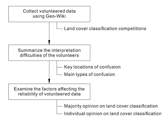
In this paper, we analysed the reliability of volunteered land cover reference data at a global scale using both consensus-based methods and expert review with two main aims. The first is to gain a better understanding of where volunteers had difficulties in visual interpretation, as formulated in these two research questions: (1) What are the areas where the largest interpretation difficulties occur and why? (2) What are the land cover types with the largest interpretation difficulties and why? The second aim is to examine the factors that affect the reliability of the volunteered land cover reference data when (1) using a consensus-based approach; and (2) considering only individual contributions. The results from these four analyses can be used to provide guidance for future data collection campaigns and can provide further insights into which data filtering methods should be used based on the needs of the user. The data used in this study were collected from land cover validation competitions that were run using the Geo-Wiki crowdsourcing tool and is outlined in the next section.
2. Data
Geo-Wiki is an online platform for the visualization, crowdsourcing and validation of global land cover maps [10,26]. As part of the crowdsourcing of global land cover, volunteers interpret very high resolution satellite imagery from Google Earth. Competitions or campaigns are used to engage volunteers to help validate different global products. During the competition, volunteers are shown different spatial locations from a sample that has been generated specifically for that competition and are then asked to interpret the land cover as well as answering other questions related to the subject of the competition.
Data used for this study came from three competitions. The first competition ran during the autumn of 2011 where volunteers were invited to help validate a map of land availability for biofuel production. This was based on a study that indicated that there are 320–1411 million hectares of land available for biofuel production in marginal lands, i.e., abandoned or degraded croplands and low productivity grasslands [27]. A random stratified sample set was generated where the strata were based on whether the locations were inside or outside of the land available for biofuel production. Volunteers were asked to interpret the land cover type and the degree of human impact at each sample location. This competition is referred to here as the “Land Availability Competition” and the user interface is shown in Figure 1. In total, 53,278 validation records were collected at around 36 K unique locations from 67 volunteers. Since the competition was concerned with the land availability for biofuel production, the sample units were mainly concentrated in agricultural regions, e.g., the Great Plains in North America, southern Europe, southwestern Russia, the Ukraine, the Sahel, Ethiopia, South Africa, India, and eastern China.
The second data source for this study is from a competition that ran in 2012 to validate locations where there was a disagreement between three different land cover products: GLC2000, MODIS, and GlobCover.
Both the GLC2000 and MODIS products were resampled to match the 300-m resolution of GlobCover and a random stratified sample was generated based on the disagreement between the three products. The volunteers were asked to identify the percentage of different land cover types at each location. This competition is referred to here as the “Product Disagreement Competition” and the user interface is shown in Figure 2. Data from the Land Availability and Product Disagreement competitions are freely available for download from the PANGAEA repository [28].
The third data source is from a special competition that was held during the Young Scientist Summer Program (YSSP) at the International Institute for Applied System Analysis (IIASA) in 2012, referred to here as the “YSSP Competition”. During the summer of 2012, the following data were collected from 16 YSSP volunteers: 1559 point validation records; 2445 records of 250 × 250-m pixel validations; and 2979 records of 1 × 1 km pixels. The 16 volunteers were all Ph.D. students undertaking research in the areas of global change, energy, ecosystem services and management, atmospheric pollution, and related disciplines. The sample locations were selected from a global land cover validation data set [29] and were assigned to each volunteer following specific rules (as outlined in more detail below).
3. Methods
3.1. Determining Key Locations of Confusion in the Volunteered Reference Data
The difficulty in validating the land cover type and the percentage coverage of each type in a given pixel at a given location can be reflected by the degree of inconsistency among different volunteers. If the land cover types are difficult to distinguish or the percent coverage is hard to estimate, the volunteers may provide very different answers, which leads to greater inconsistency in the data. Determining where the largest inconsistencies among volunteers occur can provide important guidance in future data collection campaigns.
Each sample location in the data set was validated by 1 to 41 volunteers. We only analyzed sample locations with five or more validation records, to reduce the errors caused by accidental factors, e.g., the sample is difficult to interpret but happens to be visited by a volunteer. In order to facilitate the analysis, each validation record was converted to a 10-dimensional vector (see Figure 3), i.e., the ith element in the vector was assigned the coverage of land cover class i estimated by the volunteer ().
The Euclidean distances between each pair of 10-dimensional vectors for the same sample location were then calculated. The interpretation consistency among different volunteers was measured by the average of these Euclidean distances. Since each ecoregion has unique physical conditions (including differences in geology, climate, vegetation, hydrology, and soil types) and human–earth relationships, the spatial variation in the interpretation consistency was evaluated by averaging the interpretation consistency of all sample locations within each ecoregion.
3.2. Understanding the Main Types of Land Cover Confusion in the Volunteered Reference Data
Understanding the land cover types that are confused the most often in volunteered reference data can help to increase the interpretation accuracy of the volunteers, e.g., through provision of targeted training and instruction materials aimed at helping to discriminate between confusing land cover types.
To explore the pairs of land cover types with the most confusion by the volunteers, a confusion matrix was built. It is assumed that the dominant choice of the group (i.e., the land cover type chosen most frequently by the volunteers) is true, since we do not have expert validations for the complete sample. The confusion matrix is calculated as follows: The total number of volunteers validating one sample location is denoted by . The dominant choice of the volunteers is denoted by land cover class m. The number of volunteers choosing each land cover class was calculated iteratively. For example, there are volunteers who agreed on land cover class n, which means the percentage of volunteers choosing land cover class n is , denoted by . The elements of this confusion matrix A are calculated as follows:
where k is the total number of sample locations. The result quantitatively reports the confusion level of one land cover class in relation to all the other classes, which can be a good basis for providing prior knowledge or tutorials for the volunteers in differentiating between the most confusing land cover types.
3.3. Reliability of Majority Opinion on Land Cover Classification
How to aggregate individual validations (or opinions) to characterize the views of a group and assess the reliability of the group opinion (or majority) is another important issue to be discussed in the construction of a volunteered land cover reference data set. The simplest method is to choose the majority as the group opinion. Using this approach, we want to determine if this group opinion is reliable and how many people are needed to select the most common choice.
To answer these questions, we extracted a total of 7072 records from the volunteers that were at the same location as the 299 expert control points. Logistic regression was then applied with two predictor variables: the percentage of volunteers selecting the most-commonly-identified land cover type for each location, and the self-evaluated uncertainty of the volunteers. For example, if there are 24 people who classified the sample location No. 1971, among which 20 identified it as a “Mosaic of cultivated and managed/natural vegetation”, then the percentage of volunteers selecting the most-commonly-identified land cover type is 83.33% (i.e., 20 out of 24). Since each record has a field of self-evaluated uncertainty provided by the volunteer, they were assigned a score of “0” for sure, “10” for quite sure, “20” for less sure and “30” for unsure. The self-evaluated uncertainty was also aggregated by averaging the scores of all volunteers classifying the same location. For the dependent variable, we used the occurrence of the agreement between the most commonly identified land cover type and the control point interpreted by the experts as our measure of group reliability, which is coded as “0” (for non-agreement) and “1” (for agreement). The models were built separately for the control points with and without availability of very high resolution images on Google Earth, since the very high resolution images were the basis of interpretation and uncertainty assessment of the volunteers.
3.4. Reliability of Individual Classifications of Land Cover
In this section we address the next research question, i.e., what are the factors influencing the reliability of individual classifications of land cover? To answer this question, we designed a special competition during the YSSP at IIASA in 2012 using the Geo-Wiki platform. IIASA’s annual three-month YSSP attracts Ph.D. students from around the world with different research interests. All 48 young scientists (referred to as YSSPers hereafter) were invited to participate in the competition after taking part in a training on satellite image interpretation.
The YSSPers had various professional backgrounds although their summer research projects were all closely related to the dynamics of global change. Their backgrounds can be roughly grouped into the following categories: natural resources (e.g., agronomy, forestry, energy and resources, environmental sciences), biological sciences (e.g., ecology, zoology), earth sciences (e.g., geography), social sciences (e.g., economics, management), and engineering (e.g., chemical engineering, civil engineering).
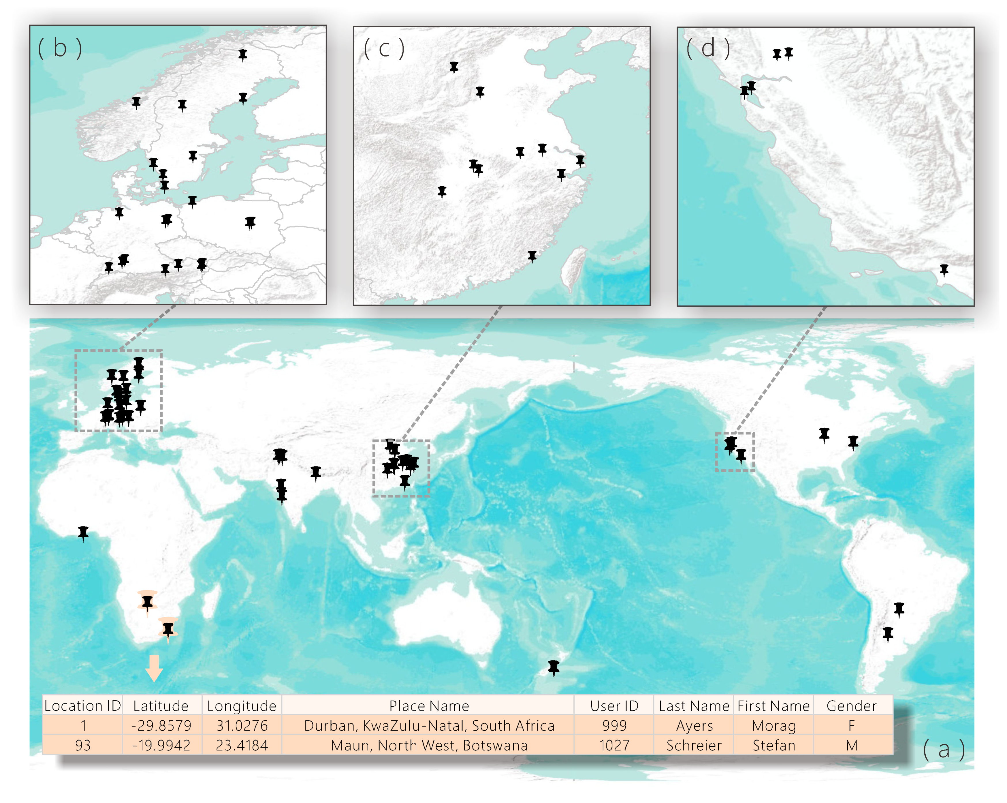
Since the YSSPers are from different places around the world, each of them was asked to provide the names of places with which they are familiar. The place names were converted into geographic coordinates using the Google Maps Geocoding API and a geodatabase was then generated containing all the familiar places of the volunteers. Limited by the number of volunteers contributing to this competition, the points were unevenly distributed globally (see Figure 4a), concentrated in central and northern Europe (Figure 4b), eastern China (Figure 4c), and the western coast of North America (Figure 4d).
Each of the volunteers was assigned a series of samples to classify, which included samples both far from and near to the volunteer’s familiar places. The minimum distance between the sample and each familiar place of the volunteer who classified the sample was calculated for each data record. The distance was calculated using the geographic coordinates of the two locations, regardless of the topographic relief of the Earth’s surface. For example, we have a volunteer who was born in Wolkersdorf, Austria, and is studying in Bremen, Germany. He spent a long vacation in Maun, Botswana. Hence, he provided the names of these three places as his familiar places. Among the samples assigned to him, we found sample X in Germany (latitude/longitude coordinates: 53.19°N/8.95°E). The minimum distance between the sample location and the volunteer’s familiar place is then the distance between sample X and Bremen, which is approximately 15.76 km. We also found sample Y (latitude/longitude coordinates: 33.81°S/25.58°E) in South Africa, and similarly, the minimum distance was calculated between sample Y and Maun, which is 1552.55 km.
Since land cover conditions can be very different due to a variety of climates even across short distances, we considered climate conditions as a factors influencing the reliability of individual classifications of land cover. We chose the Köppen–Geiger climate classification system [30], described by a code of three letters. The first letter is the general type, i.e., (A) equatorial climates; (B) arid climates; (C) warm temperate climates; (D) snow climates; and (E) polar climates. The second letter describes the precipitation regime, namely (W) desert; (S) steppe; (f) fully humid; (s) summer dry; (w) winter dry; and (m) monsoonal. The third letter corresponds to temperature, in particular, (h) hot arid; (k) cold arid; (a) hot summer; (b) warm summer; (c) cool summer; (d) extremely continental; (F) polar frost; and (T) polar tundra.
Based on the Köppen–Geiger climate classification map, we extracted the climate classes of each volunteer’s familiar places as well as the climate class of each sample that was classified. The climate class of the volunteer’s familiar place and the samples classified were compared based on the three aspects described above, i.e., the general type, the precipitation regime, and the temperature class. A new field was added to the attribute table indicating whether there was a match between the climate class of the volunteers’ familiar places and the classified samples.
To evaluate the performance of the volunteers, we prepared a marking scheme by asking experts at IIASA to interpret the satellite imagery acquired at the same time as the ones interpreted by the volunteers. The first three major land cover types and their area proportion in a 250-m-resolution pixel around each sample location were recorded. The number of land cover types is a measure of the land cover complexity for a sample location. The classification results of all volunteers were scored according to their performance in both identifying the land cover type and estimating the area proportion. If is an array of suggested land cover classes (ranked in descending order of area proportion) interpreted by the experts, then is the corresponding area proportion of each class. After the sample was validated by a volunteer, we had a record of and representing the land cover classes and their area proportion interpreted by the volunteer (the order of the land cover classes was changed to best match the order of the three land cover classes in ). The final score for a given data record is the weighted mean of the scores calculated for all land cover classes in , which was determined by the volunteer’s performance in both identifying the land cover class (i.e., the basic score, calculated by ) and by estimating the area proportion of the land cover class (i.e., the bonus score, calculated by ), weighted by the area proportion:
The basic score can range from 0 to 100, where 0 is incorrect and 100 is correct. If the volunteer provides an incorrect answer but it is highly confused with the correct answer, the volunteer will obtain a basic score (less than 30) depending on the difficulty in differentiating between the land cover classes. For example, if a sample contains a rice field and is labeled as cropland, then the volunteer will get 100 basic points for this record. The volunteer will obtain a score of 30 if it is labeled as a water body when the field is flooded before being drained. The volunteer will obtain a score of 20 if it is labeled as grassland because these two land cover types can be easily confused because of similarities in the spectral characteristics.
The bonus score ranges between 1 and 2, reflecting the volunteer’s accuracy in estimating the area proportion. For example, if the area proportion of a specific land cover class was 80% as interpreted by the experts but the volunteer said it was 70%, then the bonus score is calculated as .
The validation score can be influenced by both internal and external factors. The internal factors are related to the knowledge base of the volunteers, including the professional background of the volunteers, the minimum distance between the target sample and the familiar places of the volunteers, and whether the climate type of the target sample is included in the familiar climate types of the volunteers. The external factors can affect the interpretation difficulty of the target sample, including the main land cover type of the target sample, and the number of land cover types in the target sample. Data pre-processing included data normalization and the transformation of the categorical predictors. The contribution of different factors to the volunteer’s interpretation performance was compared by building a generalized linear regression model. We also used box plots to display the differences in the data distributions arising from each of these factors.
4. Results and Discussion
4.1. Determining Key Locations of Confusion in the Volunteered Reference Data
The spatial variation of the interpretation measured by Euclidean distances is shown in Figure 5.
The most inconsistent interpretation of the volunteers occurs in the ecoregions of tropical forests, boreal forests/taiga, tundra, grasslands, and shrublands. To uncover the reasons for this high inconsistency, typical samples were analyzed in each ecoregion.
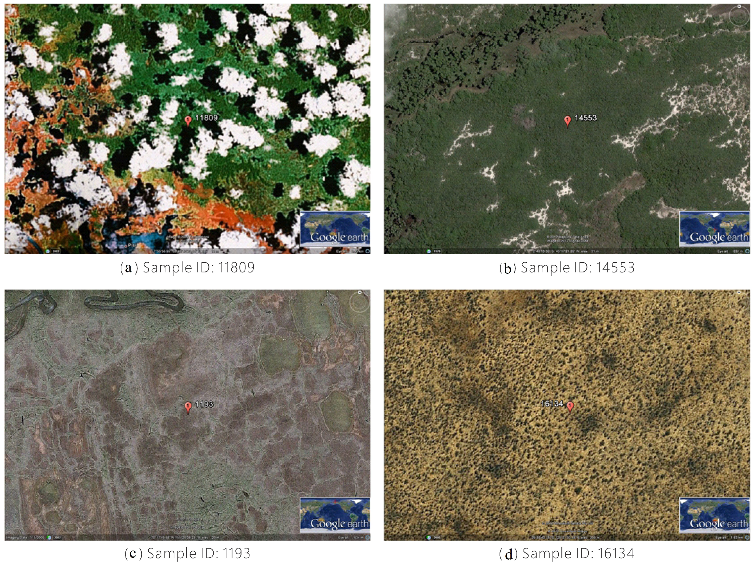
In tropical forests, cloud-free high resolution satellite images are hard to obtain. Moreover, many of the images in these locations are of Landsat resolution, which makes the interpretation difficult. For example, Figure 6a shows a validation sample located in the southern New Guinea freshwater swamp forests. Not only is there considerable cloud cover and shadow, but the image is from Landsat (i.e., TerraMetrics 15-m resolution base imagery), which has the lowest resolution provided on Google Earth. Of all of the interpretation records at this location, only 40% of the volunteers reached an agreement and categorized the location as forests, while others selected shrublands or grasslands. Some volunteers even made the mistake of judging the clouds as snow cover. This shows that Landsat resolution reference data may lead to considerable confusion in land cover classification, especially in tropical and high latitude areas, which could be largely avoided by adding more very high spatial resolution imagery or microwave data. In addition, basic knowledge of land cover interpretation (e.g., clouds can be distinguished from snow through nearby shadows) should be part of training materials presented to the volunteers to help them get started and avoid simple mistakes such as this.
The unique characteristics of specific ecoregions are also sources of confusion. Figure 6b shows a typical site in the northeastern Brazilian Restingas, a distinct ecoregion with sandy, acidic, and nutrient-poor soils. The trees are medium-sized and mixed with shrubs, which results in serious confusion over trees and shrubs during the interpretation process by the volunteers. Tundra is particularly difficult since it is highly unlikely that the volunteers have visited these regions before. The vegetation is composed of some shrub-formed trees, dwarf shrubs, grasses, mosses, and lichens, varying with a slight difference in climate and topographic condition. Figure 6c shows a typical point in the tundra where volunteers had different opinions regarding the land cover type, i.e., they chose wetlands, herbaceous cover, shrub cover, and barren areas. For samples in specific ecoregions, volunteers need greater background knowledge and spectral signatures, or alternatively these points could be assigned to volunteers with knowledge of these ecoregions.
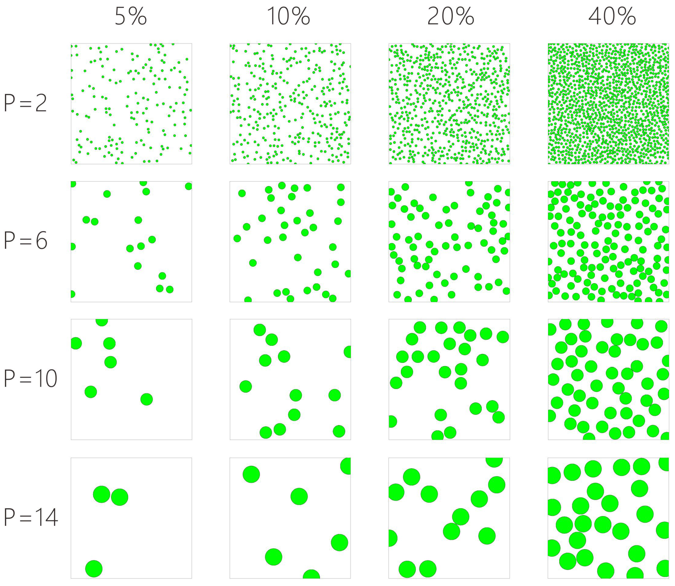
High inconsistency is also detected in the savanna, the transitional zone between forest and prairie or steppe (see Figure 6d). Since the majority of rainfall is confined to one season, the land cover varies considerably with the phenological changes in the vegetation. During the dry season, many savannas are covered with dry shrubs and grass, which are difficult to distinguish from barren land through image interpretation alone. One solution that has since been implemented in Geo-Wiki more recently is the ability to view NDVI profiles from Landsat, MODIS and PROBA-V at any location. This new tool can be used to help the volunteers distinguish between vegetation and barren land. In addition, it is difficult for the volunteers to estimate the percentage of trees or shrubs in a pixel. If the trees or shrubs are densely distributed in part of the target pixel, the coverage could be estimated more easily with the help of the grids provided on the Geo-Wiki user interface, while if the trees or shrubs are scattered over the whole target pixel (as shown in Figure 6d), estimation of the percent coverage becomes very difficult. Moreover, the presence of shadows from the vegetation canopy makes the interpretation even more difficult and the volunteers tend to over-estimate the coverage of trees or shrubs when their distribution is disperse. One solution to this problem is to develop more tools to assist the volunteers in estimating the coverage of vegetation with unified standards. A series of computer-simulated legends with different average crown diameters and canopy coverages could assist volunteers in better estimating the coverage of the vegetation. Figure 7 shows a 100 × 100-m quadrat with the average crown diameter and canopy coverage changing. Based on the actual crown diameter in the sample, the volunteers should select the right simulated legend as a reference. The legend can be plotted more accurately by making the crown sizes of trees and shrubs follow a specific distribution determined by the parameters provided by the volunteers. These types of visual aids could help to improve the classification experience of the volunteers and make it easier to estimate percentage coverage by trees or shrubs.
4.2. Understanding the Main Types of Land Cover Confusion in the Volunteered Reference Data
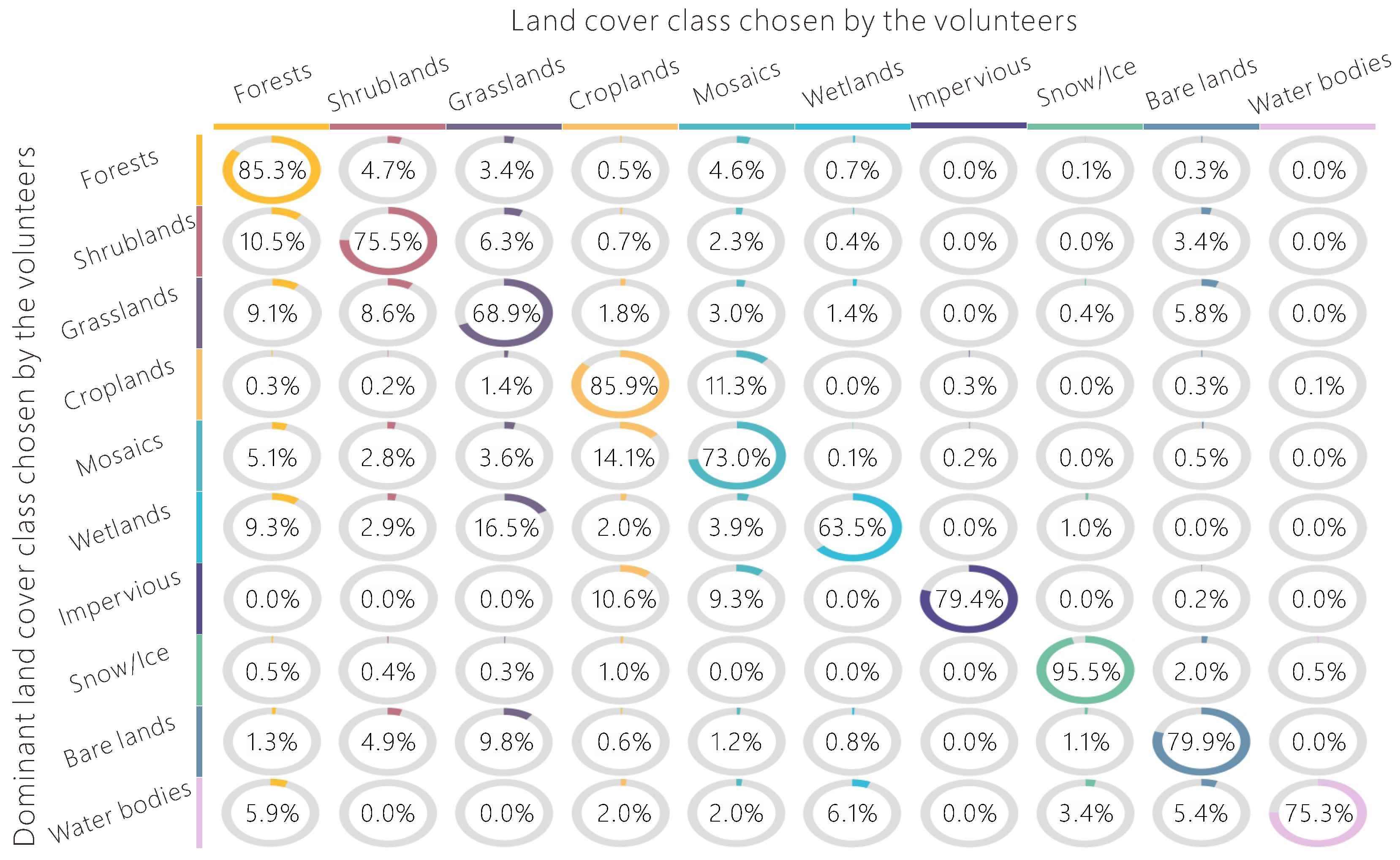
As shown in Figure 8, volunteers are good at identifying forests, snow/ice, and croplands, but have much more difficulty with grasslands and wetlands. Shrublands are confused with forests most often, with a percentage of confusion up to 10.5%, followed by confusion with grasslands. Croplands are often confused with mosaics of croplands and natural vegetation, mainly because croplands are fragmented in many regions, exposing the problem of the mismatch between the spatial resolution of the classification scheme and the sample size used in the interpretation. Wetlands are the most confusing land cover type for the volunteers, especially with grasslands and forests. The first reason is most likely due to the fact that the volunteers have less knowledge about wetlands compared to other land cover types. The second reason is that marshlands and swamp forests have similar appearances to grasslands and forests, respectively. A solution would be to provide additional data to improve the visual interpretation, e.g., the water supply, topographic conditions, soil characteristics, and groundwater levels.
Since the land cover types with the most confusion vary greatly with different vegetation landscapes, the confusion matrix was calculated for each biome separately. As an example, in Figure 9, the confusion matrix of Biome 4 (temperate broadleaf and mixed forests) was compared with Biome 8 (temperate grasslands, savannas, and shrublands), and we found that the land cover types with the most confusion were quite different. In particular, 34.4% of shrublands are misclassified as forests in Biome 4, but the percentage is only 8.3% in Biome 8. One possible reason is that the shrubs are taller in Biome 4, but small and thorny in Biome 8 to adapt to the hot and dry environment of this area. Data on canopy height and geo-tagged photographs would be useful for better differentiation of shrubs and trees in Biome 4. There is almost no confusion between grasslands and barren lands in Biome 4, but 7.7% of grasslands are mistakenly identified as barren lands in Biome 8, due to the seasonal variation of precipitation. The grasslands look drab and lifeless during the dry season so it is easy to confuse them with barren lands, while the rainy season is the best time for differentiation from barren lands. Thus, we need to provide multi-temporal images to the volunteers and geo-tagged photographs, where available, to avoid this kind of confusion, as well as the NDVI tool mentioned above.
4.3. Reliability of Majority Opinion on Land Cover Classification
The coefficients, standard errors, the z-statistic, and the associated p-values of the logistic regression models are shown in Table 1.
The results of the logistic regression show that the reliability of majority opinion on land cover classification is positively related to the percentage of volunteers selecting the most commonly identified land cover type and negatively related to the average of self-evaluated uncertainty for the sample locations where very high resolution images are available on Google Earth. The logistic regression coefficients give the change in the log odds ratio of the most common choice being reliable for a one-unit increase in the predictor variable. For every one unit increase in the percentage of volunteers selecting the most common choice, the log odds ratio of this most-commonly-identified choice being reliable increases by 0.057. Meanwhile, every one unit increase in the average of self-evaluated uncertainty decreases the log odds ratio by 0.704. Interpreting the table in the same way, for the points where very high resolution imagery is not available in Google Earth, the percentage of volunteers selecting the most common choice is also statistically significant, but the average of the uncertainty is not. The self-evaluated uncertainty of the volunteers is not significantly related to the reliability of the most common land cover choice, because it is hard for the volunteers to evaluate their uncertainty on interpretation without the assistance of very high resolution images in Google Earth.
The predicted probabilities were computed by the logistic model with one predictor variable, holding the other one at its overall mean (see Figure 10). This model can help us to roughly evaluate the reliability of the aggregated group opinion. For areas where very high resolution imagery was available in Google Earth, we found a positive correlation between the reliability of the group opinion and the percentage of volunteers selecting the most commonly identified land cover choice. If more than 36.731% of volunteers select the most commonly identified choice, holding the average self-evaluated uncertainty at its mean (1.715), the probability of this choice being correct reaches 0.8. We also found a negative correlation between the reliability of the group opinion and the average self-evaluated uncertainty of the volunteers. Similarly, if the average of the volunteers’ self-evaluated uncertainty is higher than 2.167, meaning that the volunteers are less confident about their choice, holding the percentage of the most common choice at its mean (42.344%), the probability of this choice being correct will drop down to 0.8. However, to our surprise, for the areas where very high resolution imagery is not available on Google Earth, the probability is even higher if people are less sure, but this was not statistically significant. With these models, we can predict the reliability of the group decision for each sample point using the predictor variables. The sample points with lower reliability should be excluded from the data set to potential users of the data, and they should be classified again by the experts or by more volunteers.
4.4. Reliability of Individual Classifications of Land Cover
According to the p-values in the regression model between the interpretation reliability and the predictor variables, we can see that the most statistically significant predictor variables are the complexity and the main land cover type of the target sample, followed by the variables of the volunteer’s familiar climate type and their discipline of study, where the p-values are lower than the common alpha level of 0.05.
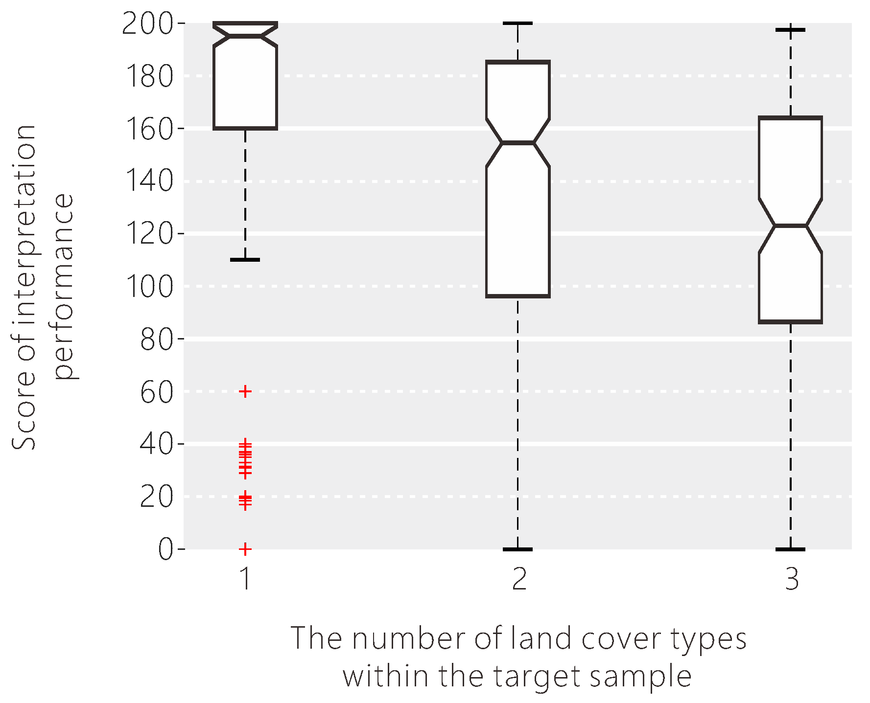
From the boxplots presenting the differences in the data distributions arising from all factors, the factors of the target sample are the most important in the interpretation performance of all individuals. The first factor that may affect the interpretation performance is the complexity of the target sample. Figure 11 shows the distribution of scores for different complexities of the target sample. When the number of land cover types within the target grid increases (from left to right in Figure 11), the median of the scores decreases, and the variation of the scores increases as well. This means that the target sample is more difficult for the volunteers to interpret when it is more complex. These more complex samples can be found by overlaying the existing very high resolution land cover products with the target grids and calculating the land cover types in each of the grids, which should then be double-checked by experts or more volunteers.
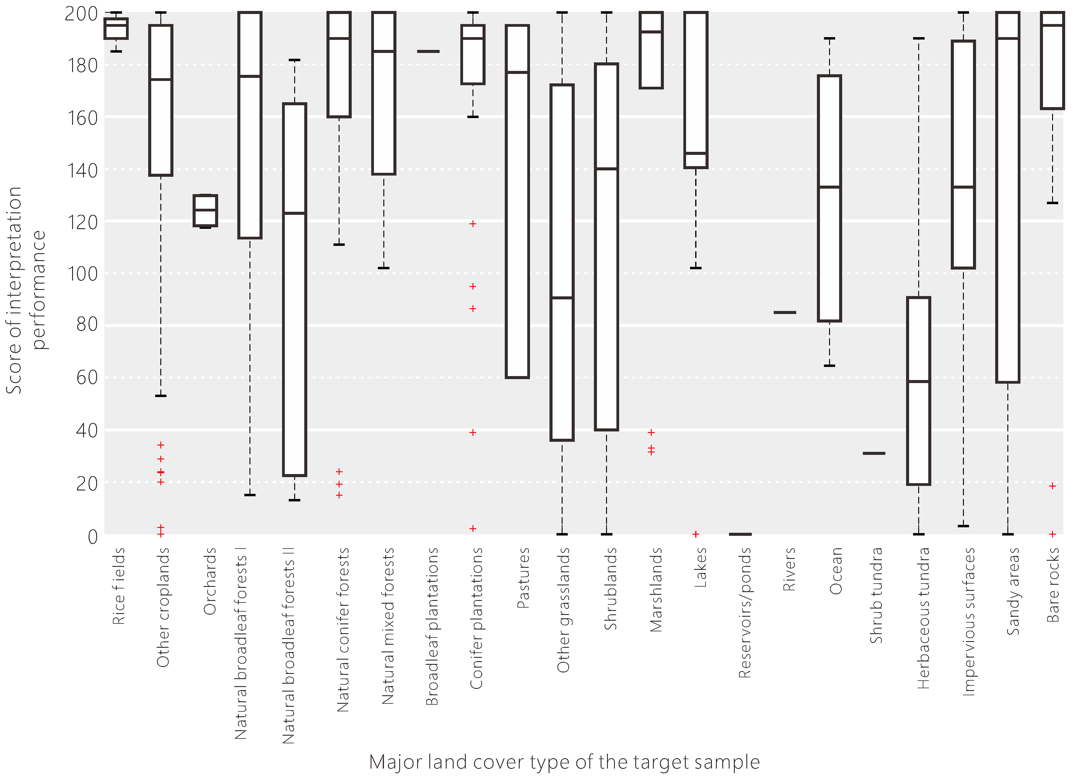
The interpretation scores are also greatly affected by the major land cover type of the target sample (see Figure 12). From this result, we can see that the volunteers are good at interpreting land cover types like croplands, forests, wetlands, water bodies, and barren lands. Some land cover types (e.g., rice fields and wetlands) are regarded as difficult-to-interpret types by experts due to their seasonally dynamic changes and differing appearances on satellite images, but the volunteers have relatively good performance in identifying them, which is unexpected. Although pastures and sandy areas have a high median score, the interquartile range is large, meaning that the volunteers have uneven performance in identifying these types, which may be affected by their prior knowledge. For example, many volunteers from eastern Asia have no idea about pastures. Some land cover types are endemic and untraversed (e.g., tundra only occurs in the high latitudes or alpine areas), so most of the volunteers had poor performances on these land cover types. Moreover, some land cover types are defined according to the canopy coverage, so the interpretation scores are spread out with a high variation.
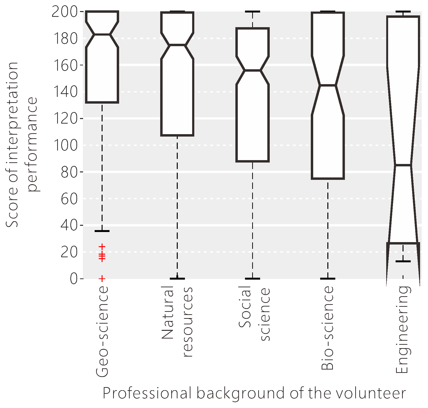
Different volunteers have their own knowledge base, because of their individual backgrounds and circumstances. Identifying the influence of the individual knowledge base of the volunteers on land cover classification is highly desirable for providing further important guidance in the data collection process. By analysing the classification performance of the volunteers with different professional backgrounds (see Figure 13), we found that the volunteers studying earth science had the highest scores, followed by natural resources. The median scores for the volunteers in these two categories are both over 180, meaning that they provide accurate land cover reference data, possibly because they have a better understanding of the definition, characteristics, distribution of the land cover types and know more about remote sensing. The median scores for the volunteers studying biosciences and social sciences are between 140 and 160, with relatively higher variation. The volunteers with an engineering background had the poorest performance among all the volunteers, with a median score of just over 80 and a very high variation. If we collect the background information of all volunteers, we can conduct a preliminary evaluation of the reliability of individual results to help in filtering out data with lower performance or for weighting the results when applied in further classification exercises.
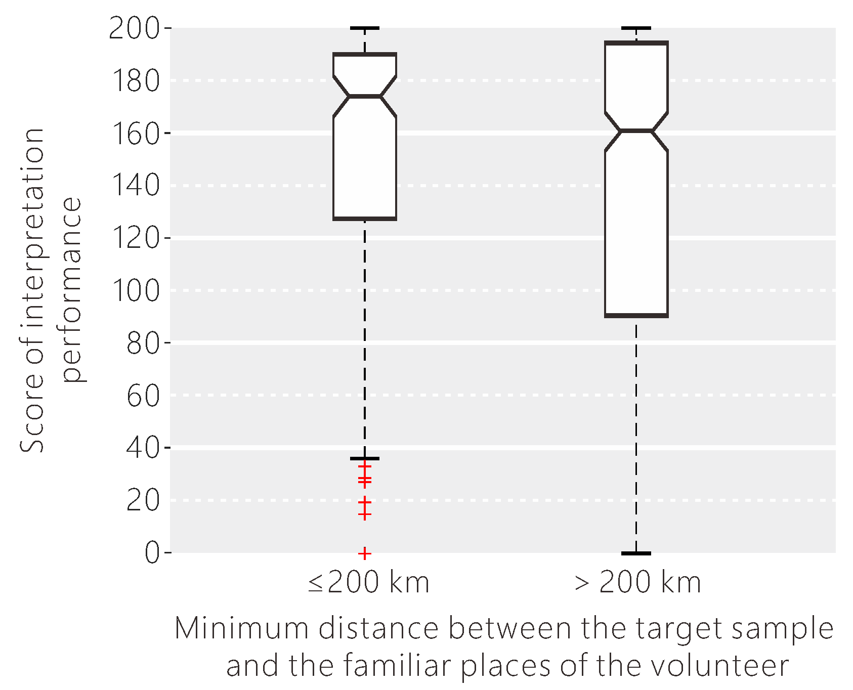
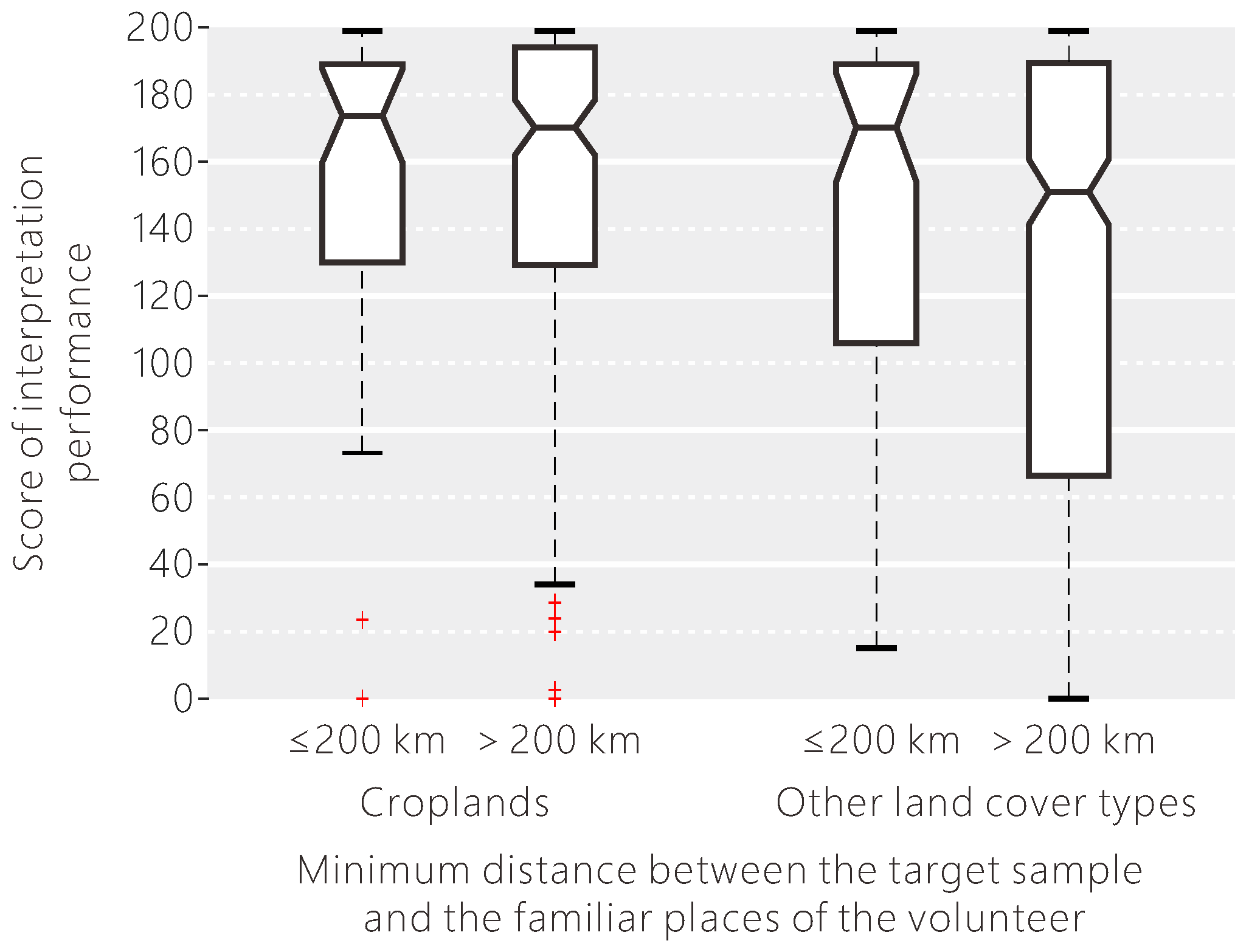
In addition to professional background, the living environment and travel experiences may also affect the classification performance of the volunteers. We examined if the volunteers were better at interpreting samples nearer to familiar places. According to the result shown in Figure 14, when the target sample was close to one of the familiar places of the volunteer, the interpretation uncertainty was a little lower, with a lower variance. Since the notches in the box plot do not overlap, we can conclude that the medians of these two groups do differ with 95% confidence. Since researchers have found little difference in identifying croplands between volunteers with and without local knowledge, the statistical analysis was done separately for croplands and other land cover types. We found that the impact of local knowledge in aiding interpretation performance was different between interpreting croplands and other land cover types. From Figure 15, the difference in the interpretation score as a result of local knowledge was larger when the volunteers were asked to identify other land cover types than croplands.
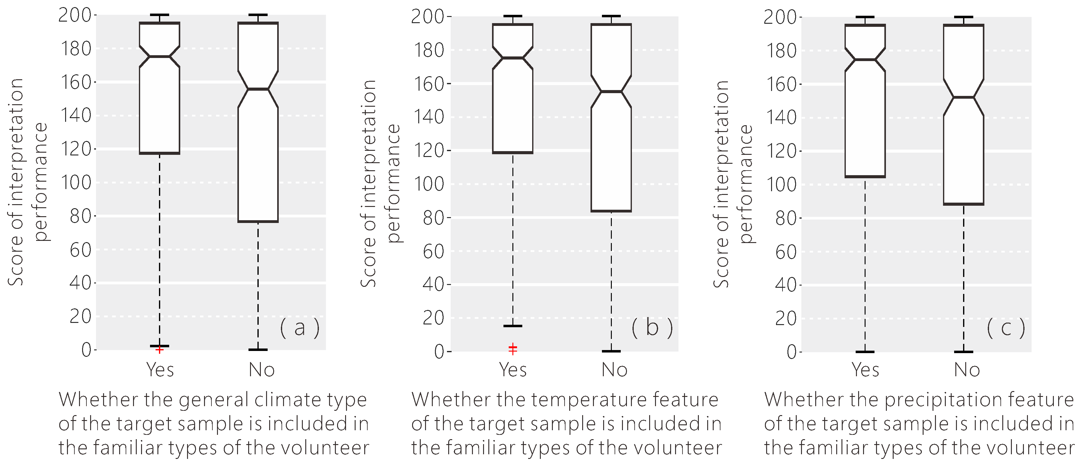
Places may have different land cover characteristics determined by climate, even if they are very close. According to Figure 16, if the climate type of the target sample, including (a) the general climate type, (b) the temperature class and, (c) the precipitation regime, is in the familiar types of the volunteer, then the interpretation performance is significantly higher than the others, and the variance is larger. Therefore, when the volunteer is familiar with the climate type of the target sample, they appear to be providing more reliable data. With the background information of the volunteer’s familiar climate type, we can provide relevant samples to the most appropriate volunteers.
5. Conclusions and Recommendations
Volunteered land cover reference data have the potential to provide useful information for land cover mapping. The key issue of using volunteered land cover reference data is to assess and improve the currently unknown reliability. In this research, volunteered data were collected via the Geo-Wiki platform and analysed to find out which areas and land cover types are the most difficult to interpret by the volunteers. We also tried to determine the factors influencing the reliability of majority opinion and the individual classifications of the volunteers with respect to land cover classification. Several recommendations are proposed to improve the collection of volunteered land cover reference data. The key conclusions and recommendations of this research are shown as follows with respect to:
(1) Difficult-to-interpret areas: The highest interpretation inconsistency of the volunteers occurs in the ecoregions of tropical and boreal forests (areas with relatively poor coverage of very high resolution images), the tundra (a unique region that the volunteers are unacquainted with), and the savanna (transitional zones). For tropical and high latitude areas, data collection can be improved by offering more very high resolution images to the volunteers where available, e.g., through Bing in addition to Google Earth. For unique ecoregions like the tundra, more background knowledge can be provided in a tutorial to help the volunteers in their interpretation. For transitional zones, where it is hard for the volunteers to estimate the canopy coverage, computer-simulated legends can help to assist the interpretation of the percentage coverage.
(2) Difficult-to-interpret land cover types: The volunteers are good at identifying forests, snow/ice, and croplands, but not grasslands and wetlands. The most confusing pairs of land cover types captured here were shrublands vs. forests and wetlands vs. grasslands among others. Moreover, the confusing pairs vary greatly with different biomes. Providing interpretation keys for both of the confusing land cover types captured by this study will help to improve future volunteer classifications.
(3) Factors influencing the reliability of the majority opinion: When very high resolution images were available on Google Earth, the reliability of the majority opinion was significantly positively correlated with the percentage of volunteers selecting the majority land cover type and negatively related to the average of self-evaluated uncertainty. This model can be used to estimate the reliability of the majority land cover type, and the more reliable samples can be used with higher priority or weighting, while the less reliable samples should be reviewed by remote sensing experts directly or by additional volunteers to see if the percentage of volunteers selecting the majority land cover type can be increased.
(4) Factors influencing the reliability of individual classifications: The interpretation score of individual volunteers is influenced by external factors (i.e., factors related to the interpretation difficulty of the target sample) and internal factors (i.e., factors related to the knowledge base of the volunteers). External factors play a more important role than the internal factors. For external factors, the interpretation score decreases with increasing complexity of the target sample and with specific land cover types (e.g., tundra, grasslands). For internal factors, volunteers with a professional background in earth sciences or natural resources have better interpretation performance, and the volunteers are good at interpreting samples near their familiar places or samples with their familiar climate type. The difference in the interpretation performance as a result of local knowledge was larger when the volunteers were asked to identify land cover types other than croplands. Therefore, more information about the volunteers should be collected when they sign up for a campaign, such as their professional background and places they are familiar with, from which familiar climate types can then be derived. We can then estimate the reliability of individual data records and select the best ones to use for a given application, or target the samples that are most appropriate for a volunteer based on the factors identified in this study.
In addition to gamification, the use of mobile apps is another increasingly popular method of crowdsourced data collection (e.g., [31]). The volunteer can easily take a photograph of the landscape using their mobile phone and upload the geo-tagged photos to a photograph repository such as Flickr or the Geo-Wiki Pictures branch. For vegetated land cover types, close-up photographs of the dominant plant species are also encouraged to help with identifying plant species (e.g., Leafsnap [32]) in order to enrich the reference database. The conclusions we obtained from this study can also guide the data collection process by mobile apps in the future. When the user is faced with areas that are difficult to interpret, the app could send push notifications to the user, requesting them to collect additional data on this area. Several different images can be prepared in advance that show the most difficult-to-interpret land cover types for each biome. Then when the user has problems choosing between two land cover choices, they can simply choose the image that most resembles what they see from a gallery of examples. The request for labelling the same target sample can also be pushed to many different volunteers, allowing for a majority result. The reliability of the majority result can be evaluated using similar methods as described in this paper. The request can also be pushed to the mobile device of specific volunteers according to their knowledge base as reflected by their user profile.
Another important issue related to the reliability of the volunteered land cover reference data is the mismatch between what people see from remote sensing imagery and what they see on the ground. Nagendra et al. [33] analyzed the difficulties that arise from this kind of misunderstanding and have provided recommendations for tackling this problem. The scale of ground features also needs to be matched to the spatial resolution of the remotely sensed images. The relationship between remote sensing data of different spatial resolutions and their potential use in mapping thematic ground features has also been summarized in Nagendra et al. [33], Nagendra and Rocchini [34], and Pettorelli et al. [35]. Therefore, we should provide more standard practice and training using examples from remote sensing. A good example would be to use the Land Use Cover Area Frame Survey (LUCAS) data set [36], which provides a set of ground-based photographs (taken in four cardinal directions and at the location) with corresponding detailed land cover and land use classes. Satellite imagery at different resolutions could then be provided with these photographs to help train the volunteers in recognizing different features at different spatial resolutions. Where possible, we should present the volunteers with remote sensing imagery at the most appropriate spatial resolution to improve their validation performance.
Finally, we have not discussed how the crowdsourced land cover reference data might be used in an actual accuracy assessment. Rather, we have provided a method to generate probabilities of accuracy based on majority opinion and self-evaluated uncertainty as well as other relationships between accuracy and different user and location-based variables. It would be possible to use such information in an approach similar to Sarmento et al. [37], which allows for the incorporation of uncertainty in the accuracy assessment of land cover. Either the self-evaluated uncertainty could be used directly as a measure of confidence, or the probability of accuracy generated by the logistic regression approach could be used as a proxy for confidence. Further research in this area is still needed.
Acknowledgments
This work was conducted based on data gathered during the Young Scientist Summer Program (YSSP) in 2012 at the International Institute for Applied Systems Analysis (IIASA), which was funded by the National Natural Science Foundation of China. The authors gratefully acknowledge the contribution of all YSSP participants in the data collection process.
Author Contributions
P.G. came up with the theme of this research and supervised this project. Y.Z. conceived and designed the experiments. Y.Z., D.F., and L.Y. analyzed the data. C.P. programmed the Geo-Wiki interface for the three different competitions and supplied the data for further analysis. L.S. and S.F. supervised the research project of Y.Z. during the YSSP period at IIASA and contributed to the ideas for the experiments. Y.Z. wrote the paper. Other authors provided edits and comments to the paper.
Conflicts of Interest
The authors declare no conflict of interest.
References
- Grafius, D.R.; Corstanje, R.; Warren, P.H.; Evans, K.L.; Hancock, S.; Harris, J.A. The impact of land use/land cover scale on modelling urban ecosystem services. Landsc. Ecol. 2016, 31, 1509–1522. [Google Scholar] [CrossRef]
- Teixeira, R.F.; de Souza, D.M.; Curran, M.P.; Antón, A.; Michelsen, O.; i Canals, L.M. Towards consensus on land use impacts on biodiversity in LCA: UNEP/SETAC Life Cycle Initiative preliminary recommendations based on expert contributions. J. Clean. Prod. 2016, 112, 4283–4287. [Google Scholar] [CrossRef]
- Tompkins, A.M.; Caporaso, L. Assessment of malaria transmission changes in Africa, due to the climate impact of land use change using Coupled Model Intercomparison Project Phase 5 earth system models. Geospat. Health 2016, 11, 380. [Google Scholar] [CrossRef] [PubMed]
- Goodchild, M.F. Citizens as sensors: The world of volunteered geography. GeoJournal 2007, 69, 211–221. [Google Scholar] [CrossRef]
- De Albuquerque, J.P.; Almeida, J.P.; Fonte, C.C.; Cardoso, A. How volunteered geographic information can be integrated into emergency management practice? First lessons learned from an urban fire simulation in the city of Coimbra. In Proceedings of the 13th International Conference on Information Systems for Crisis Response and Management (ISCRAM 2016), Rio de Janeiro, Brazil, 22–25 May 2016. [Google Scholar]
- Goodchild, M.F.; Glennon, J.A. Crowdsourcing geographic information for disaster response: A research frontier. Int. J. Digit. Earth 2010, 3, 231–241. [Google Scholar] [CrossRef]
- Hung, K.C.; Kalantari, M.; Rajabifard, A. Methods for assessing the credibility of volunteered geographic information in flood response: A case study in Brisbane, Australia. Appl. Geogr. 2016, 68, 37–47. [Google Scholar] [CrossRef]
- Attard, M.; Haklay, M.; Capineri, C. The potential of volunteered geographic information (VGI) in future transport systems. Urban Plan. 2016, 1. [Google Scholar] [CrossRef]
- Herrick, J.E.; Urama, K.C.; Karl, J.W.; Boos, J.; Johnson, M.V.V.; Shepherd, K.D.; Hempel, J.; Bestelmeyer, B.T.; Davies, J.; Guerra, J.L.; et al. The global Land-Potential Knowledge System (LandPKS): Supporting evidence-based, site-specific land use and management through cloud computing, mobile applications, and crowdsourcing. J. Soil Water Conserv. 2013, 68, 5A–12A. [Google Scholar] [CrossRef]
- Fritz, S.; McCallum, I.; Schill, C.; Perger, C.; See, L.; Schepaschenko, D.; Van der Velde, M.; Kraxner, F.; Obersteiner, M. Geo-Wiki: An online platform for improving global land cover. Environ. Model. Softw. 2012, 31, 110–123. [Google Scholar]
- Fonte, C.C.; Bastin, L.; See, L.; Foody, G.; Lupia, F. Usability of VGI for validation of land cover maps. Int. J. Geogr. Inf. Sci. 2015, 29, 1269–1291. [Google Scholar] [CrossRef]
- Laso Bayas, J.C.; See, L.; Fritz, S.; Sturn, T.; Perger, C.; Dürauer, M.; Karner, M.; Moorthy, I.; Schepaschenko, D.; Domian, D.; et al. Crowdsourcing In-Situ Data on Land Cover and Land Use Using Gamification and Mobile Technology. Remote Sens. 2016, 8, 905. [Google Scholar] [CrossRef]
- See, L.; Fritz, S.; Dias, E.; Hendriks, E.; Mijling, B.; Snik, F.; Stammes, P.; Vescovi, F.D.; Zeug, G.; Mathieu, P.P.; et al. Supporting earth-observation calibration and validation: A new generation of tools for crowdsourcing and citizen science. IEEE Geosci. Remote Sens. Mag. 2016, 4, 38–50. [Google Scholar] [CrossRef]
- Arsanjani, J.J.; Helbich, M.; Bakillah, M. Exploiting volunteered geographic information to ease land use mapping of an urban landscape. In Proceedings of the International Archives of the Photogrammetry, Remote Sensing and Spatial Information Sciences, London, UK, 21–24 May 2013; pp. 29–31. [Google Scholar]
- Liu, X.; Long, Y. Automated identification and characterization of parcels with OpenStreetMap and points of interest. Environ. Plan. B Plan. Des. 2016, 43, 341–360. [Google Scholar] [CrossRef]
- Johnson, B.A.; Iizuka, K.; Bragais, M.A.; Endo, I.; Magcale-Macandog, D.B. Employing crowdsourced geographic data and multi-temporal/multi-sensor satellite imagery to monitor land cover change: A case study in an urbanizing region of the Philippines. Comput. Environ. Urban Syst. 2017, 64, 184–193. [Google Scholar] [CrossRef]
- See, L.; Schepaschenko, D.; Lesiv, M.; McCallum, I.; Fritz, S.; Comber, A.; Perger, C.; Schill, C.; Zhao, Y.; Maus, V.; et al. Building a hybrid land cover map with crowdsourcing and geographically weighted regression. ISPRS J. Photogramm. Remote Sens. 2015, 103, 48–56. [Google Scholar] [CrossRef] [Green Version]
- Schepaschenko, D.; See, L.; Lesiv, M.; McCallum, I.; Fritz, S.; Salk, C.; Moltchanova, E.; Perger, C.; Shchepashchenko, M.; Shvidenko, A.; et al. Development of a global hybrid forest mask through the synergy of remote sensing, crowdsourcing and FAO statistics. Remote Sens. Environ. 2015, 162, 208–220. [Google Scholar] [CrossRef]
- Foody, G.M.; Boyd, D.S. Exploring the potential role of volunteer citizen sensors in land cover map accuracy assessment. In Proceedings of the 10th International Symposium on Spatial Accuracy Assessment in Natural Resources and Environmental Science (Accuracy 2012), Florianopolis, Brazil, 10–13 July 2012; pp. 203–208. [Google Scholar]
- Comber, A.; See, L.; Fritz, S.; Van der Velde, M.; Perger, C.; Foody, G. Using control data to determine the reliability of volunteered geographic information about land cover. Int. J. Appl. Earth Obs. Geoinf. 2013, 23, 37–48. [Google Scholar]
- Salk, C.F.; Sturn, T.; See, L.; Fritz, S.; Perger, C. Assessing quality of volunteer crowdsourcing contributions: lessons from the Cropland Capture game. Int. J. Digit. Earth 2016, 9, 410–426. [Google Scholar] [CrossRef] [Green Version]
- Allahbakhsh, M.; Benatallah, B.; Ignjatovic, A.; Motahari-Nezhad, H.R.; Bertino, E.; Dustdar, S. Quality control in crowdsourcing systems: Issues and directions. IEEE Internet Comput. 2013, 17, 76–81. [Google Scholar] [CrossRef]
- See, L.; Comber, A.; Salk, C.; Fritz, S.; van der Velde, M.; Perger, C.; Schill, C.; McCallum, I.; Kraxner, F.; Obersteiner, M. Comparing the quality of crowdsourced data contributed by expert and non-experts. PLoS ONE 2013, 8, e69958. [Google Scholar] [CrossRef] [PubMed]
- Salk, C.; Sturn, T.; See, L.; Fritz, S. Local knowledge and professional background have a minimal impact on volunteer citizen science performance in a land-cover classification task. Remote Sens. 2016, 8, 774. [Google Scholar] [CrossRef] [Green Version]
- Comber, A.; Mooney, P.; Purves, R.S.; Rocchini, D.; Walz, A. Crowdsourcing: It Matters Who the Crowd Are. The Impacts of between Group Variations in Recording Land Cover. PLoS ONE 2016, 11, e0158329. [Google Scholar] [CrossRef] [PubMed]
- See, L.; Fritz, S.; Perger, C.; Schill, C.; McCallum, I.; Schepaschenko, D.; Duerauer, M.; Sturn, T.; Karner, M.; Kraxner, F.; et al. Harnessing the power of volunteers, the internet and Google Earth to collect and validate global spatial information using Geo-Wiki. Technol. Forecast. Soc. Chang. 2015, 98, 324–335. [Google Scholar] [CrossRef] [Green Version]
- Cai, X.; Zhang, X.; Wang, D. Land availability for biofuel production. Environ. Sci. Technol. 2010, 45, 334–339. [Google Scholar] [CrossRef] [PubMed]
- Fritz, S.; See, L.; Perger, C.; Mccallum, I.; Schill, C.; Schepaschenko, D.; Duerauer, M.; Karner, M.; Dresel, C.; Laso-Bayas, J.C.; et al. A global dataset of crowdsourced land cover and land use reference data. Sci. Data 2017, 4, 170075. [Google Scholar] [CrossRef] [PubMed]
- Zhao, Y.; Gong, P.; Yu, L.; Hu, L.; Li, X.; Li, C.; Zhang, H.; Zheng, Y.; Wang, J.; Zhao, Y.; et al. Towards a common validation sample set for global land-cover mapping. Int. J. Remote Sens. 2014, 35, 4795–4814. [Google Scholar] [CrossRef]
- Rubel, F.; Kottek, M. Observed and projected climate shifts 1901–2100 depicted by world maps of the Köppen-Geiger climate classification. Meteorol. Z. 2010, 19, 135–141. [Google Scholar] [CrossRef]
- Herrick, J.E.; Beh, A.; Barrios, E.; Bouvier, I.; Coetzee, M.; Dent, D.; Elias, E.; Hengl, T.; Karl, J.W.; Liniger, H.; et al. The Land-Potential Knowledge System (LandPKS): Mobile apps and collaboration for optimizing climate change investments. Ecosyst. Health Sustain. 2016, 2. [Google Scholar] [CrossRef] [Green Version]
- Kumar, N.; Belhumeur, P.; Biswas, A.; Jacobs, D.; Kress, W.; Lopez, I.; Soares, J. Leafsnap: A computer vision system for automatic plant species identification. In Proceedings of the Computer Vision–ECCV 2012, Florence, Italy, 7–13 October 2012; pp. 502–516. [Google Scholar]
- Nagendra, H.; Lucas, R.M.; Honrado, J.; Jongman, R.H.G.; Tarantino, C.; Adamo, M.; Mairota, P. Remote sensing for conservation monitoring: Assessing protected areas, habitat extent, habitat condition, species diversity, and threats. Ecol. Indicators 2013, 33, 45–59. [Google Scholar] [CrossRef]
- Nagendra, H.; Rocchini, D. High resolution satellite imagery for tropical biodiversity studies: the devil is in the detail. Biodivers. Conserv. 2008, 17, 3431–3442. [Google Scholar] [CrossRef]
- Pettorelli, N.; Laurance, W.F.; Obrien, T.G.; Wegmann, M.; Nagendra, H.; Turner, W. Satellite remote sensing for applied ecologists: Opportunities and challenges. J. Appl. Ecol. 2014, 51, 839–848. [Google Scholar] [CrossRef]
- Eurostat. Overview of LUCAS; Eurostat: Luxembourg, 2015. [Google Scholar]
- Sarmento, P.; Carrao, H.; Caetano, M.; Stehman, S.V. Incorporating reference classification uncertainty into the analysis of land cover accuracy. Int. J. Remote Sens. 2009, 30, 5309–5321. [Google Scholar] [CrossRef]
Figure 1.
The user interface from the Geo-Wiki tool employed in the “Land Availability Competition”.
Figure 1.
The user interface from the Geo-Wiki tool employed in the “Land Availability Competition”.
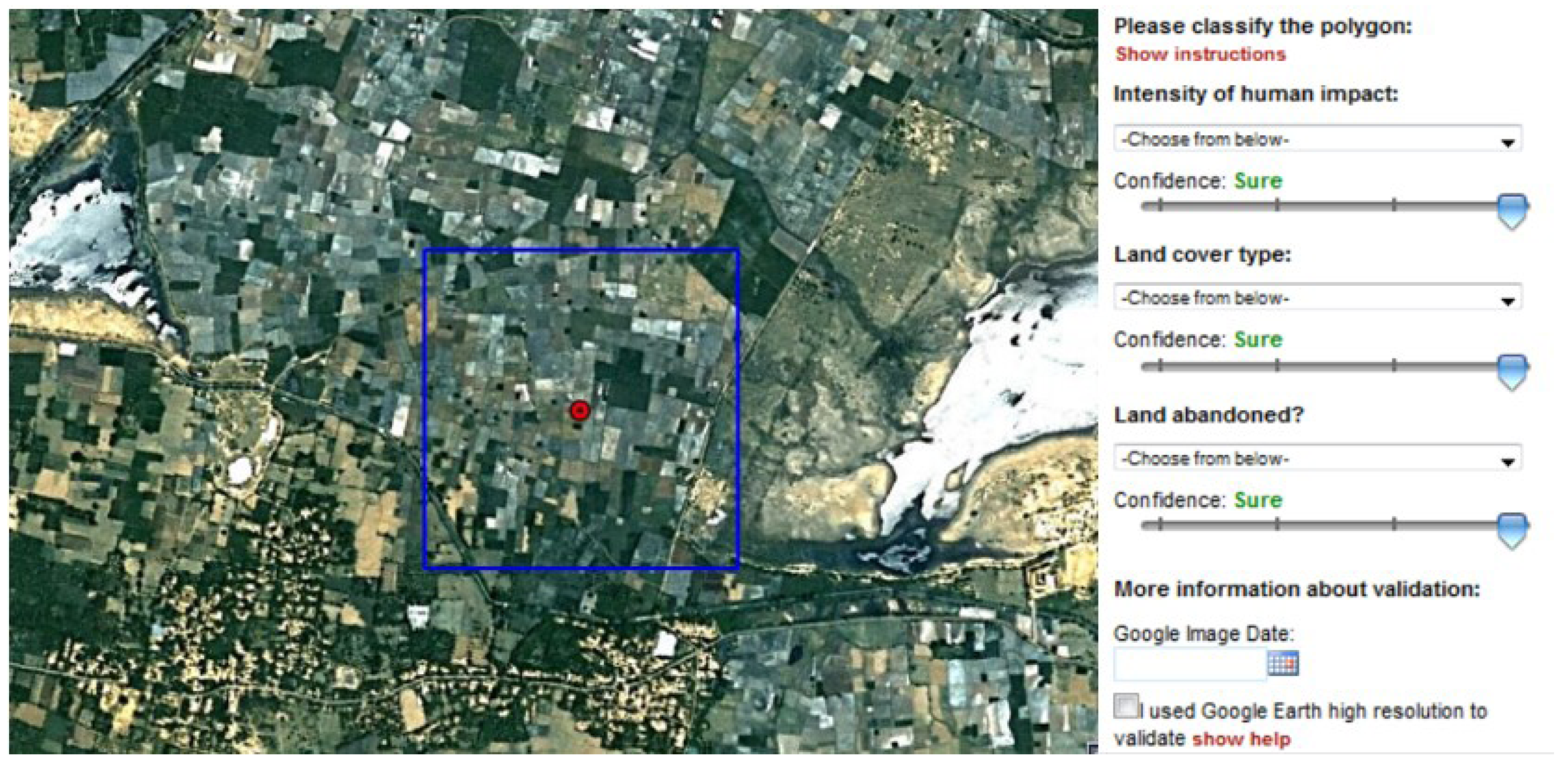
Figure 2.
The user interface from the Geo-Wiki tool employed in the “Product Disagreement Competition”.
Figure 2.
The user interface from the Geo-Wiki tool employed in the “Product Disagreement Competition”.

Figure 3.
The vectorization examples of three interpretation records from the volunteers. The numbers 1 to 10 refer to the 10 land cover classes in Geo-Wiki, while the colored cells refer to the percentage of the land cover class specified by the volunteer.
Figure 3.
The vectorization examples of three interpretation records from the volunteers. The numbers 1 to 10 refer to the 10 land cover classes in Geo-Wiki, while the colored cells refer to the percentage of the land cover class specified by the volunteer.
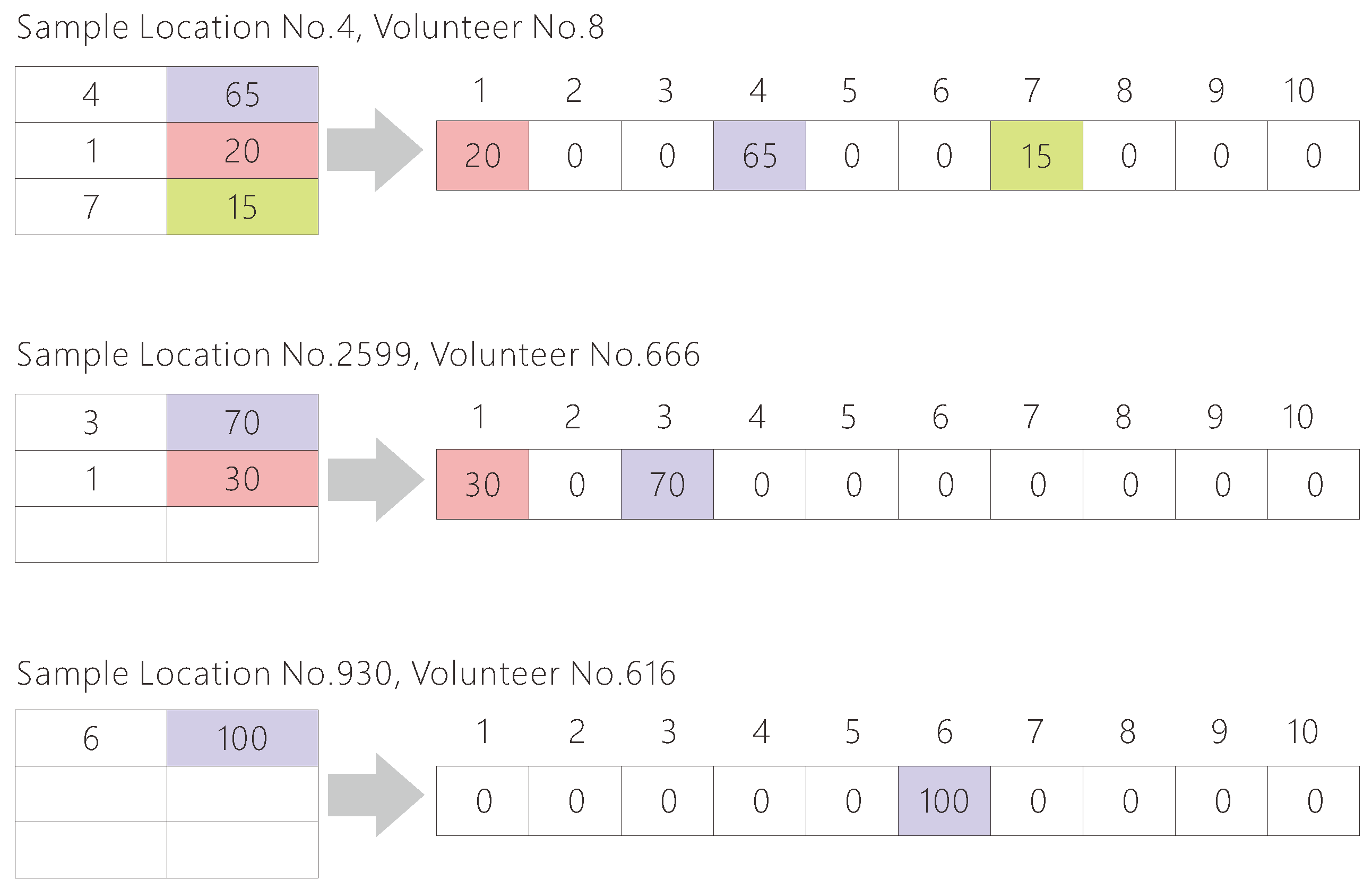
Figure 4.
(a–d) The spatial distribution of place names with which the volunteers are familiar, globally and regionally, and two records in the attribute table.
Figure 4.
(a–d) The spatial distribution of place names with which the volunteers are familiar, globally and regionally, and two records in the attribute table.

Figure 5.
Spatial variation of interpretation consistency measured by Euclidean distances.
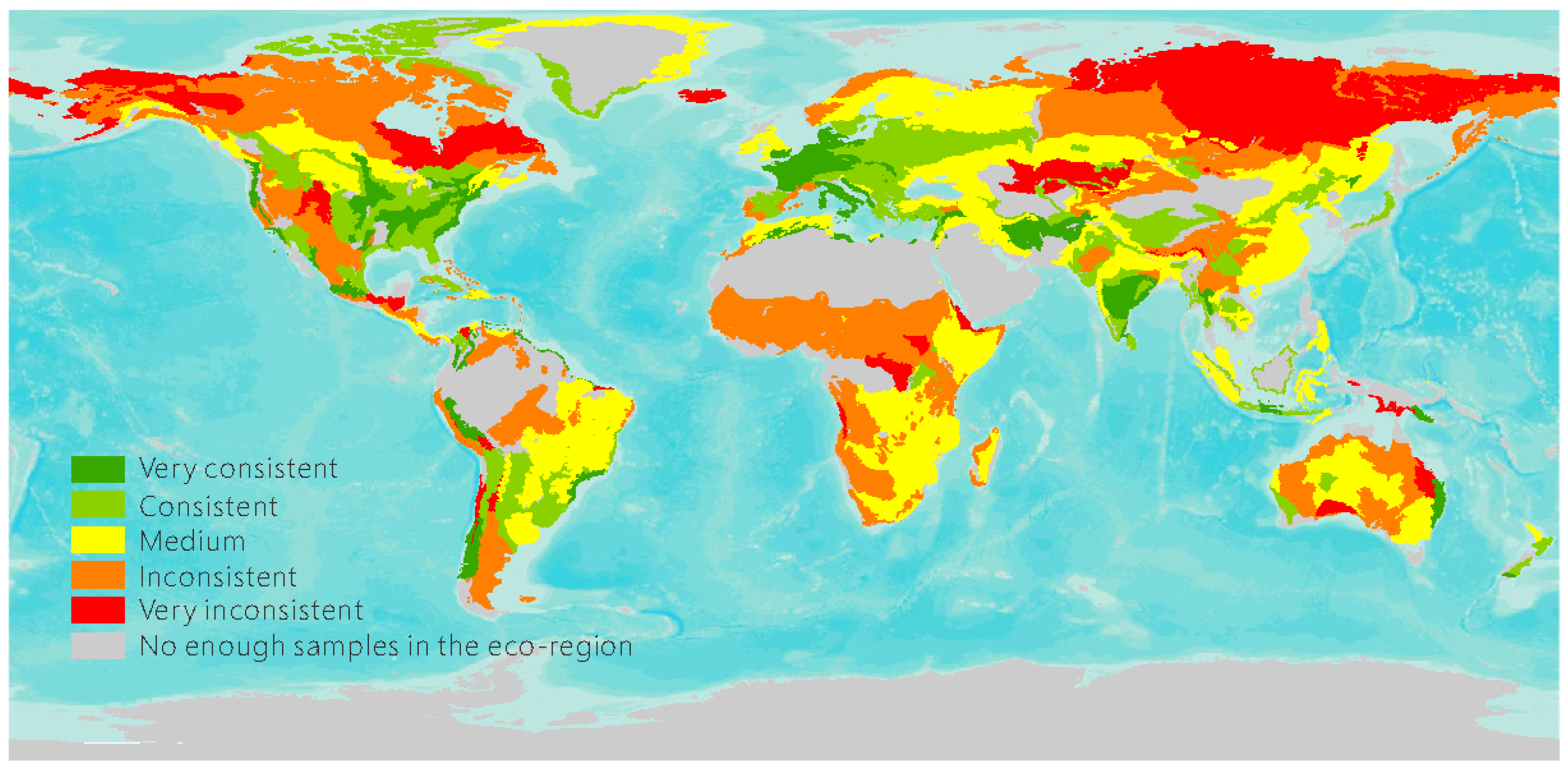
Figure 6.
(a–d) Examples of satellite imagery in Google Earth for some of the typical sample locations interpreted by the volunteers.
Figure 6.
(a–d) Examples of satellite imagery in Google Earth for some of the typical sample locations interpreted by the volunteers.

Figure 7.
Computer-simulated legends of different average crown diameter and canopy coverage to aid in visual interpretation by the volunteers.
Figure 7.
Computer-simulated legends of different average crown diameter and canopy coverage to aid in visual interpretation by the volunteers.

Figure 8.
The level of confusion by the volunteers for all land cover types based on all interpretations compared to the dominant land cover type chosen.
Figure 8.
The level of confusion by the volunteers for all land cover types based on all interpretations compared to the dominant land cover type chosen.

Figure 9.
The level of confusion by volunteers of all land cover types in two different biomes.

Figure 10.
Probabilities of the majority land cover choice being correct estimated using logistic regression models with the predictor variable of (a) percentage of volunteers selecting the most commonly identified land cover choice (for areas where very high resolution images are available); (b) average self-evaluated uncertainty of volunteers (for areas where very high resolution images are available); (c) percentage of volunteers selecting the most commonly identified land cover choice (for areas where very high resolution images are unavailable); (d) average self-evaluated uncertainty of volunteers (for areas where very high resolution images are unavailable).
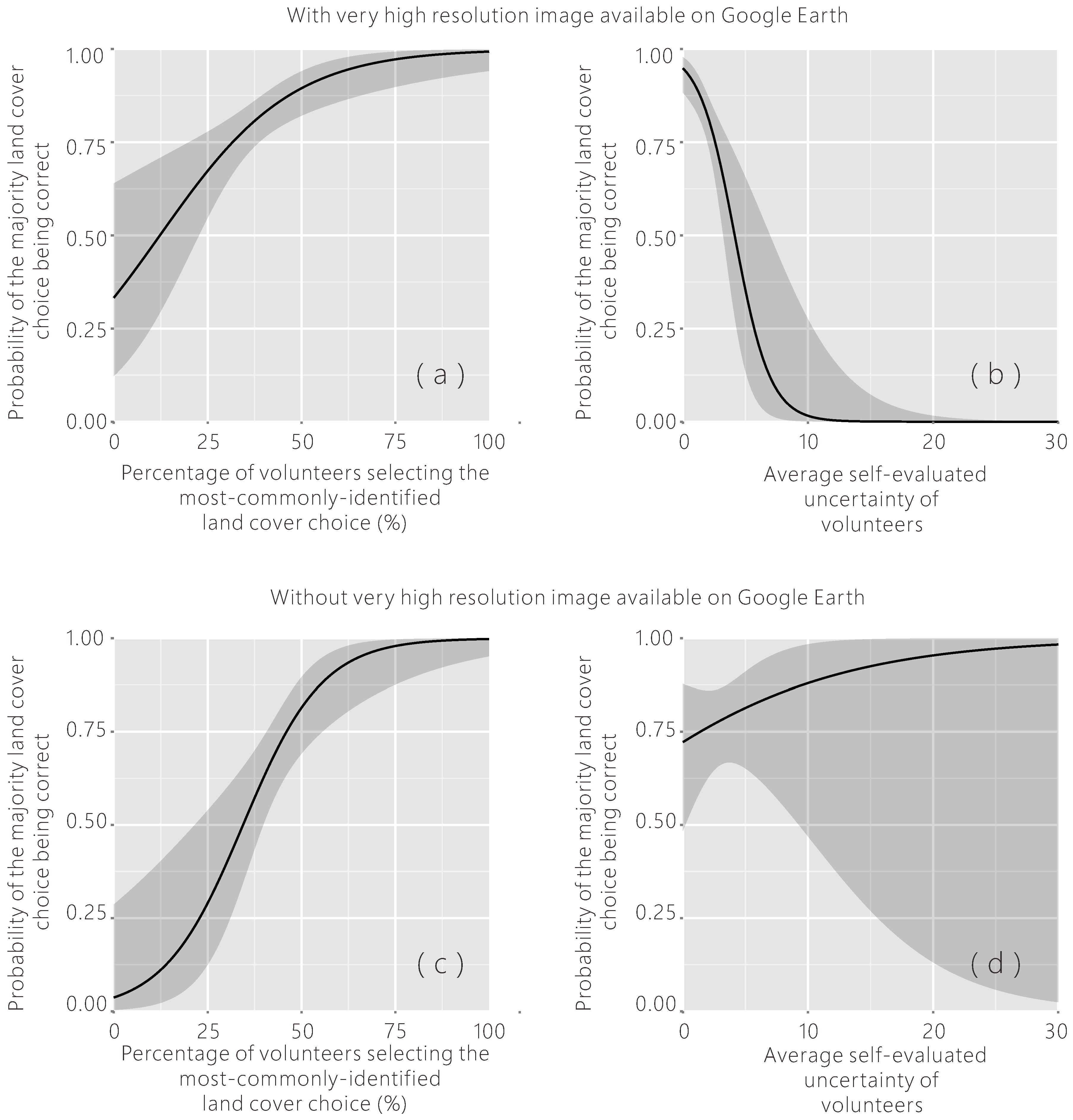
Figure 11.
The influence of the target sample complexity on the interpretation performance of the volunteers.
Figure 11.
The influence of the target sample complexity on the interpretation performance of the volunteers.

Figure 12.
The influence of the major land cover types of the target sample on the interpretation performance of the volunteers.
Figure 12.
The influence of the major land cover types of the target sample on the interpretation performance of the volunteers.

Figure 13.
The influence of the professional background of the volunteer on their interpretation performance.
Figure 13.
The influence of the professional background of the volunteer on their interpretation performance.

Figure 14.
The influence of the minimum distance between the target sample and the familiar places of the volunteer on their interpretation performance.
Figure 14.
The influence of the minimum distance between the target sample and the familiar places of the volunteer on their interpretation performance.

Figure 15.
The influence of the minimum distance between the target sample and the familiar places of the volunteer on their interpretation performance displayed separately for croplands and other land cover types.
Figure 15.
The influence of the minimum distance between the target sample and the familiar places of the volunteer on their interpretation performance displayed separately for croplands and other land cover types.

Figure 16.
(a–c) The influence of the volunteer’s familiar climate type on the interpretation performance.
Figure 16.
(a–c) The influence of the volunteer’s familiar climate type on the interpretation performance.


Table 1.
Coefficients and associated statistical values of the logistic regression models.
| Estimated Std. | Error | Z Value | Pr (>|z|) | |
|---|---|---|---|---|
| Very high resolution imagery available on Google Earth | ||||
| (Intercept) | 0.511 | 0.761 | 0.671 | 0.50211 |
| Dominant percentage | 0.057 | 0.017 | 3.294 | 0.00099 *** |
| Average uncertainty | −0.704 | 0.199 | −3.532 | 0.00041 *** |
| Very high resolution imagery not available on Google Earth | ||||
| (Intercept) | −3.592 | 1.376 | −2.610 | 0.00905 ** |
| Dominant percentage | 0.095 | 0.028 | 3.379 | 0.00073 *** |
| Average uncertainty | 0.104 | 0.146 | 0.713 | 0.47599 |
Signif.codes: ‘***’ p ≤ 0.001, ‘**’ p ≤ 0.01, ‘*’ p ≤ 0.05, ‘.’ p ≤ 0.1.
© 2017 by the authors. Licensee MDPI, Basel, Switzerland. This article is an open access article distributed under the terms and conditions of the Creative Commons Attribution (CC BY) license (http://creativecommons.org/licenses/by/4.0/).
Share and Cite
MDPI and ACS Style
Zhao, Y.; Feng, D.; Yu, L.; See, L.; Fritz, S.; Perger, C.; Gong, P. Assessing and Improving the Reliability of Volunteered Land Cover Reference Data. Remote Sens. 2017, 9, 1034. https://doi.org/10.3390/rs9101034
AMA Style
Zhao Y, Feng D, Yu L, See L, Fritz S, Perger C, Gong P. Assessing and Improving the Reliability of Volunteered Land Cover Reference Data. Remote Sensing. 2017; 9(10):1034. https://doi.org/10.3390/rs9101034
Chicago/Turabian StyleZhao, Yuanyuan, Duole Feng, Le Yu, Linda See, Steffen Fritz, Christoph Perger, and Peng Gong. 2017. "Assessing and Improving the Reliability of Volunteered Land Cover Reference Data" Remote Sensing 9, no. 10: 1034. https://doi.org/10.3390/rs9101034
Note that from the first issue of 2016, this journal uses article numbers instead of page numbers. See further details here.